Abstract

The usual $\chi^{2}$ method of fit quality assessment is a special case of the more general method of Bayesian model comparison which involves integrals of the likelihood and prior over all possible values of all parameters. We introduce new parametrisations based on systematic expansions around the stretched exponential or Fourier-transformed Lévy source distribution, and utilise the increased discriminating power of the Bayesian approach to evaluate the relative probability of these models to be true representations of a recently measured Bose-Einstein correlation data in $e^{+}e^{-}$ annihilations at LEP.

1 Bayes factors

The Bayesian definition of probability differs radically from the conventional “frequentist” one, necessitating the overhaul of many concepts and techniques used in statistics and its applications. Since its introduction in 1900 [1], the $\chi^{2}$ statistic has become the standard criterion for goodness of fit in physics and many other disciplines, while Laplace’s Bayesian approach [2] remained largely forgotten until revived by Jeffreys [3]. Later refinements such as the Maximum Likelihood occupy a middle ground between the two approaches.

In this contribution, we demonstrate the use of one Bayesian technique in the simple context of fitting or, more generally, the quantitative assessment of evidence in favour of a hypothesis $H_{1}$ as a description of given data, compared to a rival hypothesis $H_{2}$. We do so by analysing the concrete example of binned data for the correlation function $C_{2}(Q)$ in the four-momentum difference $Q=\sqrt{-(p_{1}-p_{2})^{2}}$ as published recently by the L3 Collaboration [4].

Suppose we have data ${\mathbf{D}}=\{Q_{1},\ldots,Q_{n}\}$ consisting of $n$ measurements of particle four-momentum differences, assumed to be mutually independent as is customary in femtoscopy. Typically, the experimentalist will want to test how well various parametrisations fit the data. For the purposes of Bayesian analysis, a given parametrisation $y(Q\,|\,{\bm{\theta}}_{m})$ with $N_{m}$ free parameters ${\bm{\theta}}_{m}=\{\theta_{m1},\theta_{m2},\ldots,\theta_{mN_{m}}\}$ is considered a “model” or “hypothesis” $H_{m}$. The starting point is the odds in favour of model $H_{m}$ compared to a different model $H_{\ell}$”, defined as the ratio $p(H_{m}\,|\,{\mathbf{D}})/p(H_{\ell}\,|\,{\mathbf{D}})$, while the evidence for $H_{m}$ versus $H_{\ell}$ is the logarithm of the odds. Use of Bayes’ Theorem for both hypotheses yields

$$\frac{p(H_{m}\,|\,{\mathbf{D}})}{p(H_{\ell}\,|\,{\mathbf{D}})} =\frac{p({\mathbf{D}}\,|\,H_{m})\,p(H_{m})}{\sum_{k}p({\mathbf{D}}\,|\,H_{k})\,p(H_{k})}\;\frac{\sum_{k}p({\mathbf{D}}\,|\,H_{k})\,p(H_{k})}{p({\mathbf{D}}\,|\,H_{\ell})\,P(H_{\ell})}=\frac{p({\mathbf{D}}\,|\,H_{m})}{p({\mathbf{D}}\,|\,H_{\ell})}\cdot\frac{p(H_{m})}{p(H_{\ell})}.$$ (1)

The evidence of $H_{m}$ versus $H_{\ell}$ is therefore the same as the Bayes factor $B_{m\ell}=\lg[p({\mathbf{D}}\,|\,H_{m})/p({\mathbf{D}}\,|\,H_{\ell})]$ if there is no a priori reason to prefer $H_{m}$ above $H_{\ell}$ and therefore $p(H_{m})=p(H_{\ell})=1/2$. A large Bayes factor says that the evidence for $H_{m}$ is stronger than the evidence for $H_{\ell}$ and vice versa. It can be written as a ratio of integrals over the respective parameter spaces of ${\bm{\theta}}_{m}$ and ${\bm{\theta}}_{\ell}$,

$$B_{m\ell} =\lg\frac{p({\mathbf{D}}\,|\,H_{m})}{p({\mathbf{D}}\,|\,H_{\ell})}=\lg\frac{\int d{\bm{\theta}}_{m}\;p({\mathbf{D}}|{\bm{\theta}}_{m},H_{m})\,p({\bm{\theta}}_{m}|H_{m})}{\int d{\bm{\theta}}_{\ell}\;p({\mathbf{D}}|{\bm{\theta}}_{\ell},H_{\ell})\,p({\bm{\theta}}_{\ell}|H_{\ell})}.$$ (2)

Solving the high-dimensional integrals will often be an arduous task. Fortunately, the independence of the measurements implies that the likelihood $p({\mathbf{D}}\,|\,{\bm{\theta}}_{m},H_{m})$ factorises into the product of likelihoods for individual data points, which by assumption have the same form,

$$p({\mathbf{D}}\,|\,{\bm{\theta}}_{m},H_{m})=\prod_{i}p(Q_{i}\,|\,{\bm{\theta}}_{m},H_{m})\approx[p(Q\,|\,{\bm{\theta}}_{m},H_{m})]^{n}.$$ (3)

Due to the large exponent, even the slightest nonuniformity in $p(Q\,|\,{\bm{\theta}}_{m},H_{m})$ will lead to the development of a strong peak in parameter space for the overall likelihood, situated at the maximum likelihood point $\hat{\bm{\theta}}_{m}$. An asymmetric prior $p({\bm{\theta}}_{m}\,|\,H_{m})$ will shift the peak to a value ${\bm{\theta}}_{m}^{*}$, but it will not materially affect the width of the peak or its differentiability. Unless the shifted peak falls on a boundary of the parameter space or happens to be nondifferentiable, it can therefore be expanded around ${\bm{\theta}}_{m}^{*}$ [5]:

$$p({\mathbf{D}}\,|\,{\bm{\theta}}_{m},H_{m})\,p({\bm{\theta}}_{m}\,|\,H_{m})\simeq p({\mathbf{D}}\,|\,{\bm{\theta}}^{*},H_{m})\,p({\bm{\theta}}^{*}\,|\,H_{m})\exp\left[-\frac{1}{2}({\bm{\theta}}_{m}-{\bm{\theta}}_{m}^{*}){\mathbf{A}}^{-1}({\bm{\theta}}_{m}-{\bm{\theta}}_{m}^{*})\right]$$ (4)

where ${\mathbf{A}}^{-1}$ is the Hessian of the expansion

$$A_{ij}^{-1}=-\frac{\partial^{2}\ln[p({\mathbf{D}}\,|\,{\bm{\theta}}_{m},H_{m})\,p({\bm{\theta}}_{m}\,|\,H_{m})]}{\partial\theta_{mi}\,\partial\theta_{mj}}\biggr{|}_{{\bm{\theta}}_{m}^{*}}$$ (5)

and ${\mathbf{A}}$ is the parameter covariance matrix. As more data is accumulated, the peak narrows so that we can neglect the fact that parameters may have finite ranges. Integrating the above as if it were a Gaussian, one obtains Laplace’s result [2]

$$\int_{-\infty}^{+\infty}d{\bm{\theta}}\;p({\mathbf{D}}\,|\,{\bm{\theta}}_{m},H_{m})\,p({\bm{\theta}}_{m}\,|\,H_{m}) \simeq p({\mathbf{D}}\,|\,{\bm{\theta}}_{m}^{*},H_{m})\,p({\bm{\theta}}_{m}^{*}\,|\,H_{m})\sqrt{(2\pi)^{N_{m}}\det{\mathbf{A}}_{m}}\,,$$ (6)

which under the stated assumptions is a good approximation of the full-blown integral appearing in Eq. (2) if $n\gtrsim 20N_{m}$. The Bayes factor becomes simply the difference

$$B_{m\ell} \simeq h_{\ell}-h_{m}$$ (7)

$$h_{k} \equiv-\lg\left[p({\mathbf{D}}\,|\,{\bm{\theta}}_{k}^{*},H_{k})\,p({\bm{\theta}}_{k}^{*}\,|\,H_{k})\sqrt{(2\pi)^{N_{k}}\det{\mathbf{A}}_{k}}\right].$$ (8)

Evidence $h_{k}$ can be determined for any single model $H_{k}$, but has no meaning on its own; only differences $h_{\ell}-h_{m}$ are meaningful in quantifying the probability for $H_{m}$ to be true compared to $H_{\ell}$,

$$\frac{p(H_{m}\,|\,{\mathbf{D}})}{p(H_{\ell}\,|\,{\mathbf{D}})}\simeq 2^{h_{\ell}-h_{m}}.$$ (9)

2 Relationship to $\chi^{2}$ and the Maximum Likelihood

The Bayesian results obtained above differ from the traditional Maximum Likelihood Estimate (MLE), which ignores the priors $p({\bm{\theta}}_{m}\,|\,H_{m})$ and approximates the integral (2) to the maxima of the likelihoods,

$$B_{m\ell} =\lg\frac{\int d{\bm{\theta}}_{m}\;p({\mathbf{D}}|{\bm{\theta}}_{m},H_{m})\,p({\bm{\theta}}_{m}|H_{m})}{\int d{\bm{\theta}}_{\ell}\;p({\mathbf{D}}|{\bm{\theta}}_{\ell},H_{\ell})\,p({\bm{\theta}}_{\ell}|H_{\ell})}\simeq\lg\frac{p({\mathbf{D}}|\hat{\bm{\theta}}_{m},H_{m})}{p({\mathbf{D}}|\hat{\bm{\theta}}_{\ell},H_{\ell})}.$$ (10)

The traditional $\chi^{2}$ goodness-of-fit is related to the above as follows. The measurements $\{Q_{i}\}$ are binned into bins $b=1,\ldots,B$ with bin midpoints $Q_{b}$, yielding the histogram version of the data, ${\mathbf{D}}=\{n_{b}\}_{b=1}^{B}$ with $\sum_{b}n_{b}=1$. The most general “parametrisation” of the histogram contents is then the multinomial with ${\bm{\alpha}}=\{\alpha_{b}\}_{b=1}^{B}$ the set of Bernoulli probabilities with $B-1$ degrees of freedom,

$$p({\bm{n}}\,|\,{\bm{\alpha}},n)=n!\prod_{b=1}^{B}\frac{\alpha_{b}^{n_{b}}}{n_{b}!}\,,$$ (11)

which on use of the Stirling approximation becomes, up to a normalisation constant,

$$p({\bm{n}}\,|\,{\bm{\alpha}},n) =c\cdot\exp\left[-\sum_{b}n_{b}\ln\frac{n_{b}}{n\alpha_{b}}\right].$$ (12)

Expanding the free parameters ${\bm{\alpha}}$ around the measured data ${\bm{n}}$ and truncating

$$p({\bm{n}}\,|\,{\bm{\alpha}},n) =c\cdot\exp\left[-\sum_{b}\left(\frac{(n\alpha_{b}-n_{b})^{2}}{2n_{b}}-\frac{(n\alpha_{b}-n_{b})^{3}}{3n_{b}^{2}}+\ldots\right)\right]\simeq c\cdot\exp\left[-\frac{1}{2}\sum_{b}\frac{(n\alpha_{b}-n_{b})^{2}}{n_{b}}\right],$$ (13)

we can identify the multinomial quantities with the measured correlation functions at mid-bin points $Q_{b}$ by setting $n_{b}\to I\,C_{2}(Q_{b})$, $C=\sum_{b}C_{2}(Q_{b})$, and $n\to I\,C$. The $n_{b}$ in the denominator is almost equal to the measured bin variances $n_{b}\simeq\sigma^{2}(n_{b})=I^{2}\,\sigma^{2}(C_{2}(Q_{b}))$ so that the quadratic term is

$$\frac{(n\alpha_{b}-n_{b})^{2}}{2\,n_{b}}\simeq\frac{[C_{2}(Q_{b})-y(Q_{b}\,|\,\hat{\bm{\theta}}_{m})]^{2}}{2\,\sigma(C_{2}(Q_{b}))^{2}},$$ (14)

where $n\alpha_{b}/I\to y(Q_{b}\,|\,\hat{\bm{\theta}}_{m})$, which includes all the constants, is the unnormalised parametrisation for $C_{2}(Q)$ in common use. Comparing this to the usual definition

$$\chi^{2}=\sum_{b}\frac{[C_{2}(Q_{b})-y(Q_{b}\,|\,\hat{\bm{\theta}}_{m})]^{2}}{\sigma(C_{2}(Q_{b}))^{2}},$$ (15)

we see that the maximum likelihood is approximately equal to

$$p({\mathbf{D}}|\hat{\bm{\theta}}_{m},H_{m})\simeq e^{-\chi^{2}/2},$$ (16)

so that $\chi^{2}$ is seen to be an approximation of the Bayes formulation, using only a single point in the parameter space ${\bm{\theta}}_{m}^{*}\equiv\hat{\bm{\theta}}_{m}$ and thereby effectively assuming a uniform prior. Furthermore, $\chi^{2}$ truncates the expansion of (13); this is probably the approximation most vulnerable to criticism.

3 Parametrisations and Lévy-based polynomial expansions

We now apply the above general ideas to the specific case of the various parametrisations shown in Table 1 for the correlation function data for two-jet events published by the L3 Collaboration [4]. Hypotheses $H_{1}$ to $H_{3}$ are taken from the L3 paper. Realising that it is important to quantify the degree of deviation of Bose-Einstein correlation data from the Gaussian or the exponential shape, the L3 Collaboration also studied a “Laguerre expansion” as well as the symmetric Lévy source distribution, characterized by the stretched-exponential correlation function of hypothesis $H_{2}$. In $H_{4}$ and $H_{5}$, we propose a new expansion technique that measures deviations from $H_{2}$ in terms of a series of “Lévy polynomials” that are orthogonal to the characteristic function of symmetric Lévy distributions, generalising the results presented in Ref. [6].

$$L_{1}(x\,|\,\alpha)=\det\left(\begin{array}[]{c@{\hspace*{8pt}}c}\mu_{0,\alpha}\hfil\hskip 8.0&\mu_{1,\alpha}\\ 1\hfil\hskip 8.0&x\end{array}\right)\qquad L_{2}(x\,|\,\alpha)=\det\left(\begin{array}[]{c@{\hspace*{8pt}}c@{\hspace*{8pt}}c}\mu_{0,\alpha}\hfil\hskip 8.0&\mu_{1,\alpha}\hfil\hskip 8.0&\mu_{2,\alpha}\\ \mu_{1,\alpha}\hfil\hskip 8.0&\mu_{2,\alpha}\hfil\hskip 8.0&\mu_{3,\alpha}\\ 1\hfil\hskip 8.0&x\hfil\hskip 8.0&x^{2}\end{array}\right)\qquad\text{etc.}$$ (22)

where $\mu_{r,\alpha}=\int_{0}^{\infty}dx\;x^{r}f(x\,|\,\alpha)=\tfrac{1}{\alpha}\,\Gamma(\tfrac{r+1}{\alpha})$. These reduce, up to a normalisation constant, to the Laguerre polynomials for $\alpha=1$. Figure 1 displays two examples for various values of $\alpha$. Polynomials cannot be both orthogonal and derivatives for transcendental weight functions [9], and therefore in $H_{6}$ and $H_{7}$ we also investigated nonorthogonal derivative functions of the stretched exponential.

	Hypothesis	Functional form	$N_{m}$
$H_{1}$	Gauss	$\displaystyle\gamma[1+\varepsilon Q]\,\left[1+\lambda e^{-R^{2}Q^{2}}\right]$	4
$H_{2}$	Stretched Exponential	$\displaystyle\gamma[1+\varepsilon Q]\,\left[1+\lambda e^{-R^{\alpha}Q^{\alpha}}\right]$	5
$H_{3}$	Simplified $\tau$-model	$\displaystyle\gamma[1+\varepsilon Q]\,\left[1+\lambda e^{-R^{2\alpha}Q^{2\alpha}}\cos[\tan(\alpha\pi/2)\,R^{2\alpha}Q^{2\alpha}]\right]$	5
$H_{4}$	1st-order Lévy polynomial	$\displaystyle\gamma\,\left[1+\lambda e^{-R^{\alpha}Q^{\alpha}}[1+c_{1}L_{1}(Q|\alpha,R)]\right]$	5
$H_{5}$	3rd-order Lévy polynomial	$\displaystyle\gamma\,\left[1+\lambda e^{-R^{\alpha}Q^{\alpha}}[1+c_{1}L_{1}(Q|\alpha,R)+c_{3}L_{3}(Q|\alpha,R)]\right]$	6
$H_{6}$	1st-order derivative	$\displaystyle\gamma\,\left[1+\lambda e^{-R^{\alpha}Q^{\alpha}}+c_{1}\tfrac{d}{dQ}e^{-R^{\alpha}Q^{\alpha}}\right]$	5
$H_{7}$	3rd-order derivative	$\displaystyle\gamma\,\left[1+\lambda e^{-R^{\alpha}Q^{\alpha}}+c_{1}\tfrac{d}{dQ}e^{-R^{\alpha}Q^{\alpha}}+c_{3}\tfrac{d^{3}}{dQ^{3}}e^{-R^{\alpha}Q^{\alpha}}\right]$	6

Table 1: Summary of parametrisations tested

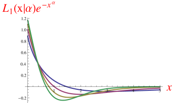
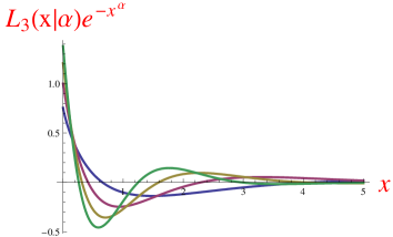
Figure 1: Lévy polynomials of first and third order times the weight function $e^{-x^{\alpha}}$ for $\alpha=0.8,1.0,1.2,1.4$.

4 Application to L3 binned data

In Table 2, we show the results of applying the Laplace approximation (6) to the L3 two-jet data, which is provided in terms of 100 binned values for the correlation function $C(Q_{b})$ together with standard errors $\sigma(C(Q_{b}))$ in the range $0<Q<4$ GeV. Throughout, we used a Gaussian prior $p({\bm{\theta}}_{m}^{*}\,|\,H_{m})$ with a width which was determined by numerical integration over one of the L3 data points. To illustrate the contributions of the likelihood, prior and determinant factors entering $h_{m}$ in (8), we have listed their logarithmic contributions separately in the three columns headed L, P and F. These quantities are therefore the building blocks for calculating the odds between any two competing hypotheses. Thus one can, for example, deduce that the odds for $H_{7}$ compared to $H_{6}$ are $2^{100.6-97.0}\simeq 12{\,:}1$. Also included in Table 2 are the traditional $\chi^{2}$ measure (C) and its associated confidence level (CL).

	Hypothesis	$N_{m}$	L		P		F		$h_{m}$		C		CL
$H_{1}$	Gauss	4	177.	8	-3.	6	32.	2	206.	5	2.	57	3.	4$\times 10^{-13}$%
$H_{2}$	Stretched Exponential	5	138.	5	-0.	5	34.	0	172.	0	2.	02	1.	5$\times 10^{-6}$%
$H_{3}$	Simplified $\tau$-model	5	68.	2	-3.	4	37.	0	101.	8	1.	00	49.	1%
$H_{4}$	1st-order Lévy polynomial	5	66.	2	2.	2	30.	3	98.	8	0.	97	57.	3%
$H_{5}$	3rd-order Lévy polynomial	6	65.	9	3.	8	41.	6	111.	3	0.	97	55.	7%
$H_{6}$	1st-order derivative	5	67.	3	4.	2	29.	1	100.	6	0.	98	53.	0%
$H_{7}$	3rd-order derivative	6	60.	4	4.	9	31.	7	97.	0	0.	89	77.	0%

Table 2: Results of fitting parametrisations listed in Table 1.

Legend:	L $\equiv-\lg P({\mathbf{D}}\,|\,{\bm{\theta}}_{m}^{*},H_{m})\equiv\chi^{2}/(2\ln 2)$	$h_{m}\equiv L+P+F$
	P $\equiv-\lg P({\bm{\theta}}_{m}^{*}\,|\,H_{m})$	C $\equiv\chi^{2}/(B-N_{m})$
	F $\equiv-\lg\sqrt{(2\pi)^{N_{m}}\det{\mathbf{A}}}$	CL $\equiv$ confidence level

It is inappropriate to generalise conclusions based on one specific dataset with its specific circumstances. The fact that in the two-jet L3 data the correlation function $C_{2}(Q)$ drops well below 1.0 for $0.5<Q<2$ GeV, for example, is probably the dominant influence on the goodness of fit. Under this caveat, we make the following observations regarding the results shown in Table 2:

1. At first sight, the Bayes factor and the $\chi^{2}$ methodologies deliver judgements which are rather similar: $H_{7}$ is consistently ranked best, while $H_{1}$ and $H_{2}$ are ranked worst (least likely). The two methodologies yield vastly different numbers when one hypothesis is bad. As shown below, there are surprising variations even among the better ones.

2. The determinant plays an important role. For example, factor F$=41.6$ for $H_{5}$ is significantly larger than that of similar models $H_{4}$ and $H_{6}$ even though the three log likelihoods are similar. This can be traced to the fact that the uncertainty in the parameters for $H_{5}$ is larger, as expressed in the width of its Gaussian (4). While $\chi^{2}$, based only on the likelihood, can hardly distinguish between $H_{4}$ and $H_{5}$, the contribution of the large $H_{5}$ determinant ensures that the Bayesian odds for $H_{4}$ versus $H_{5}$ are 5800:1. In other words, by taking into account not only the best parameter values ${\bm{\theta}}_{5}^{*}$ but also their uncertainties, the Bayes factor could distinguish what $\chi^{2}$ could not.

3. Our Bayes factor calculation takes the experimental standard errors $\sigma(C(Q_{b}))$ into account by using (14) in the exponent of the likelihood; in other words, we assume that they are Gaussian. We can improve on this approximation by doing a more complete Bayesian analysis using not the binned data but the pair momenta $\{Q_{i}\}$ themselves.

4. As Fig. 1 shows, the Lévy polynomials introduced here are well suited to describe one-sided strongly-peaked data. It may be helpful to use them, as we have done here, merely as part of parametrisations of data to which they show some resemblance. More systematic use in Gram-Charlier or other expansions will be faced with issues inherent in all asymptotic series [7, 8].

5 Conclusions

1. In hypotheses $H_{4}$ to $H_{7}$, we have presented new techniques to study deviations from a stretched exponential or Fourier-transformed Lévy shape. Details will be published elsewhere.

2. The standard measures of fit quality like $\chi^{2}$ or CL are useful in rejecting models which are inconsistent with a given dataset. Where two or more models are consistent with the data, however, they are unable to select the more probable. The Bayes factor (9) permits quantification of the evidence (relative probability) for the validity of models.

3. Besides the likelihood, the prior and determinant also play a role, sometimes decisively so.

4. The Laplace approximation (4) is usually fairly accurate, but the assumption of Gaussian errors for count data (13), which is made by truncation of the Taylor expansion in the data, is of dubious quality.

5. By integrating over parameter space, Bayesian evidence takes into account all possible values of the parameters, while $\chi^{2}$ and Maximum Likelihood do not.

6. Bayes factors depend linearly on the two priors. This is good in that they are made explicit, but bad in the sense that results can and do change depending on the choice of priors.

7. The omission of priors in $\chi^{2}$ is to its disadvantage as it discards important information.

8. It may appear that $\chi^{2}$ does not need any alternative hypothesis to be of use. This is not so, however: the alternative implicit in $\chi^{2}$ is the “Bernoulli class” of multinomials [10].

Acknowledgements: We thank the L3 collaboration for making its results available electronically [4] and the organizers of WPCF 2011 for support and an excellent atmosphere. This work was supported in part by the South African National Research Foundation and by the Hungarian OTKA grant NK–101438.

References

• [1] K.Β Pearson, On a criterion that a given system of deviations …is such that it can be reasonably supposed to have arisen in random sampling, Phil.Β Mag.Β (5) 50 (1900) 157.
• [2] P.S.Β Laplace, MΓ©moires de MathΓ©matique et de Physique, Tome SixiΓ¨me (1774).
• [3] R.Β Jeffreys, Theory of Probability, Oxford University Press (1961).
• [4] L3 Collaboration, P.Β Achard et al., Test of the $\tau$-Model of Bose-Einstein Correlations and Reconstruction of the Source Function in Hadronic $Z$-boson Decay at LEP, Eur.Β Phys. J.Β C71 (2011) 1648 [arXiv:1105.4788], see also http://l3.web.cern.ch/l3/
• [5] R.E.Β Kass and A.E.Β Raftery, Bayes Factors, J.Β American Statistical Association 90 (1995) 773.
• [6] T.Β CsΓΆrgΕ‘ and S.Β Hegyi, Model independent shape analysis of correlations in 1, 2 or 3 dimensions, Phys.Β Lett.Β B 489 (2000) 15.
• [7] M.B.Β de Kock, Gaussian and non-Gaussian-based Gram-Charlier and Edgeworth expansions for correlations of identical particles in HBT interferometry, M.Sc., University of Stellenbosch (2009).
• [8] H.C.Β Eggers, M.B.Β de Kock and J.Β Schmiegel, Determining source cumulants in femtoscopy with Gram-Charlier and Edgeworth series, Mod.Β Phys.Β Lett.Β A 26 (2011) 1771 [arXiv:1011.3950].
• [9] A.Β ErdΓ©lyi et al., Higher Transcendental Functions, Vol.Β 2, McGraw-Hill, New York (1953).
• [10] E.T.Β Jaynes, Probability Theory: The Logic of Science, Cambridge University Press (2003).