Digital Holography at Shot Noise Level

Abstract

By a proper arrangement of a digital holography setup, that combines off-axis geometry with phase-shifting recording conditions, it is possible to reach the theoretical shot noise limit, in real-time experiments. We studied this limit, and we show that it corresponds to 1 photo-electron per pixel within the whole frame sequence that is used to reconstruct the holographic image. We also show that Monte Carlo noise synthesis onto holograms measured at high illumination levels enables accurate representation of the experimental holograms measured at very weak illumination levels. An experimental validation of these results is done.

I Introduction

Demonstrated by Gabor [1] in the early 50’s, the purpose of holography is to record, on a 2D detector, the phase and the amplitude of the radiation field scattered from an object under coherent illumination. The photographic film used in conventional holography is replaced by a 2D electronic detection in digital holography [2], enabling quantitative numerical analysis. Digital holography has been waiting for the recent development of computer and video technology to be experimentally demonstrated [3]. The main advantage of digital holography is that, contrary to holography with photographic plates [1], the holograms are recorded by a photodetector array, such as a CCD camera, and the image is digitally reconstructed by a computer, avoiding photographic processing [4].

Off-axis holography [5] is the oldest configuration adapted to digital holography [6, 3, 7]. In off-axis digital holography, as well as in photographic plate holography, the reference beam is angularly tilted with respect to the object observation axis. It is then possible to record, with a single hologram, the two quadratures of the object’s complex field. However, the object field of view is reduced, since one must avoid the overlapping of the image with the conjugate image alias [8]. Phase-shifting digital holography, which has been introduced later [9], records several images with a different phase for the reference beam. It is then possible to obtain the two quadratures of the field in an in-line configuration even though the conjugate image alias and the true image overlap, because aliases can be removed by taking image differences.

With the development of CCD camera technologies, digital holography became a fast-growing research field that has drawn increasing attention [10, 11]. Off-axis holography has been applied recently to particle [12] polarization [13], phase contrast [14], synthetic aperture [15], low-coherence [16, 17] photothermal [18], and microscopic [17, 19, 20] imaging. Phase-shifting holography has been applied to 3D [21, 22], color [23], synthetic aperture [24], low-coherence [25], surface shape [26], photothermal [18], and microscopic [21, 27, 20] imaging.

We have developed an alternative phase-shifting digital holography technique that uses a frequency shift of the reference beam to continuously shift the phase of the recorded interference pattern [28]. One of the advantages of our setup is its ability to provide accurate phase shifts that allow to suppress twin images aliases [29]. More generally, our setup can be viewed as a multipixel heterodyne detector that is able of recording the complex amplitude of the signal electromagnetic field $\cal E$ in all pixels of the CCD camera in parallel. We get then the map of the field over the CCD pixels (i.e. ${\cal E}(x,y)$ where $x$ and $y$ are the pixels coordinate). Since the field is measured on all pixels at the same time, the relative phase that is measured for different locations $(x,y)$ is meaningful. This means that the field map ${\cal E}(x,y)$ is a hologram that can be used to reconstruct the field $\cal E$ at any location along the free-space optical propagation axis, in particular in the object plane.

Our heterodyne holographic setup has been used to perform holographic [28], and synthetic aperture [24] imaging. We have also demonstrated that our heterodyne technique used in an off-axis holographic configuration is capable of recording holograms with optimal sensitivity [30]. This means that it is possible to fully filter-off technical noise sources, that are related to the reference beam (i.e. to the zero order image [31]), reaching thus, without any experimental effort, the quantum limit of noise of one photo electron per reconstructed pixel during the whole measurement time.

In the present paper we will discuss on noise in digital holography, and we will try to determine what is the ultimate noise limit both theoretically, and in actual holographic experiments in real-time. We will see that, in the theoretical ideal case, the limiting noise is the Shot Noise on the holographic reference beam. In reference to heterodyne detection, we also refer to the reference beam as Local Oscillator (LO). We will see that the ultimate theoretical limiting noise can be reached in real time holographic experiments, by combining the two families of digital holography setups i.e. phase-shifting and off-axis. This combination enables to fully filter-off technical noises, mainly due to LO beam fluctuations in low-light conditions, opening the way to holography with ultimate sensitivity [30, 32].

II Off-axis + Phase-Shifting holography

In order to discuss on noise limits in digital holography, we first need to give some general information on holography principles. We will thus describe here a typical digital holographic setup, how the holographic information is obtained from recorded CCD images, and how this information is used to reconstruct holographic images in different reconstruction planes. We will consider here the case of an off-axis + phase-shifting holographic setup, able to reach the ultimate noise limit, in low-light imaging conditions, in real time.

II-A The Off-axis + Phase Shifting holography setup

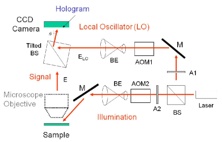
Figure 1: Digital holography setup. AOM1 and AOM2 : acousto-optic modulators; BS : beam splitter; BE : beam expander; M : mirror; A1 and A2 : attenuator; $\theta$ : tilt angle of the beam splitter with respect to optical axis

The holographic setup used in the following discussion, is presented on Fig.1. We have considered here, a reflection configuration, but the discussion will be the same in case of transmission configuration.

The main optical beam (complex field $E_{L}$, optical angular frequency $\omega_{L}$) is provided by a Sanyo (DL-7147-201) diode laser ($\lambda=658\;\rm{nm}$). It is split through a 50/50 Beam Splitter (BS) into an illumination beam ($E_{I}$,$\omega_{I}$), and a LO beam ($E_{LO}$,$\omega_{LO}$). The illumination intensity can be reduced with grey neutral filters. Both beams go through Acousto-Optic Modulators (AOMs) (Crystal Technology, $\omega_{\rm{aom1,2}}\simeq 80\;\rm{MHz}$) and only the first diffraction order is kept. In the typical experiment case considered here, the modulators are adjusted for the 4-phase heterodyne detection, but other configurations are possible (8-phases, sideband detection …). We have thus :

$$\omega_{I}=\omega_{L}+\omega_{\rm{aom2}}$$ (1)

$$\omega_{LO}=\omega_{L}+\omega_{\rm{aom1}}$$ (2)

with :

$$\omega_{I}-\omega_{LO}=2\pi f_{\rm{ccd}}/4$$ (3)

where $f_{\rm{ccd}}$ is the acquisition frame rate of the CCD (typically $12.5\;\rm{Hz}$).

The beams outgoing from the AOMs are expanded by Beam Expanders BEs. The illumination beam is pointed towards the object studied. The reflected radiation ($E$,$\omega=\omega_{I}$) and the LO beam are combined with a beam splitter, which is angularly tilted by typically $1^{\circ}$, in order to be in an Off-Axis holographic configuration. Light can be collected with an objective for microscopic imaging. Interferences between reflected light and LO are recorded with a digital camera (PCO Pixelfly): $f_{\rm{ccd}}=12.5\;\rm{Hz}$, $1280\times 1024$ pixels of $6.7\times 6.7\;\rm{\mu m}$, 12-bit.

We can notice that our Off-axis + Phase-Shifting (OPS) holographic setup, presented here, exhibits several advantages. Since we use AOMs, the amplitude, phase and frequency of both illumination and LO beams can be fully controlled. The phase errors in phase-shifting holography can thus be highly reduced [29]. By playing with the LO beam frequency , it is possible to get holographic images at sideband frequencies of a vibrating object [33, 34], or to get Laser Doppler images of a flow [35, 35], and image by the way blood flow, in vivo [36, 37, 38]. The OPS holographic setup can also be used as a multi pixel heterodyne detector able to detect, with a quite large optical étendue (product of a beam solid angular divergence by the beam area) the light scattered by a sample, and to analyze its frequency spectrum [39, 40]. This detector can be used to detect photons that are frequency shifted by an ultrasonic wave [41, 42] in order to perform Ultrasound-modulated optical tomography [43, 44, 45, 46, 47, 48].

The OPS setup benefits of another major advantage. By recording several holograms with different phases (since we do phase shifting), we perform heterodyne detection. We benefit thus on heterodyne gain. Moreover, since the heterodyne detector is multi pixels, it is possible to combine information on different pixels in order to extract the pertinent information on the object under study, while removing the unwanted technical noise of the LO beam. As we will show, because the setup is off-axis, the object pertinent information can be isolated from the LO beam noise. By this way, we can easily reach, in a real life holographic experiment, the theoretical noise limit, which is related to the Shot Noise of LO beam.

II-B Four phases detection

In order to resolve the object field information in quadrature in the CCD camera plane, we will consider, to simplify the discussion, the case of 4 phases holographic detection, which is commonly used in Phase Shifting digital holography [9].

Sequence of $4n$ frames $I_{0}$ to $I_{4n-1}$ are recorded at $12.5\;\rm{Hz}$. For each frame $I_{k}$, the signal on each pixel $I_{k,p,q}$ (where $k$ is the frame index, and $p,q$ the pixel indexes along the $x$ and $y$ directions) is measured in Digital Count (DC) units between 0 and 4095 (since our camera is 12-bit). The $1280\times 1024$ matrix of pixels is truncated to a $1024\times 1024$ matrix for easier discrete Fourier calculations. For each frame $k$ the optical signal is integrated over the acquisition time $T=1/f_{\rm{ccd}}$. The pixel signal $I_{k,p,q}$ is thus defined by :

$$I_{k,p,q}=\int_{t_{k}-T/2}^{t_{k}+T/2}dt\iint_{(p,q)}{dx}{dy}\left|E(x,y,t)+E_{LO}(x,y,t)\right|^{2}$$ (4)

where $\iint_{(p,q)}$ represents the integral over the pixel $(p,q)$ area, and $t_{k}$ is the recording time of frame $k$. Introducing the complex representations ${\cal E}$ and ${\cal E}_{LO}$ of the fields $E$ and $E_{LO}$, we get :

$$E(x,y,t)={\cal E}(x,y)e^{j\omega_{I}t}+c.c.$$ (5)

$$E_{LO}(x,y,t)={\cal E}_{LO}(x,y)e^{j\omega_{LO}t}+c.c$$ (6)

$$I_{k,p,q} =a^{2}T$$

$$\left(|{\cal E}_{p,q}|^{2}+{|\cal E}_{LO}|^{2}+{\cal E}_{p,q}{\cal E}_{LO}^{*}{\rm e}^{j\left(\omega_{I}-\omega_{LO}\right)t_{k}}+c.c.\right)$$

where $a$ is the pixel size. To simplify the notations in Eq.II-B, we have considered that the LO field ${\cal E}_{LO}$ is the same in all locations $(x,y)$, and that signal field ${\cal E}_{p,q}$ does not vary within the pixel $(p,q)$. If ${\cal E}_{LO}$ varies with location, one has to replace ${\cal E}_{LO}$ by ${\cal E}_{LO,p,q}$ in Eq.II-B.

The condition given in Eq.3 imposed a phase shift of the LO beam equal to $\pi/2$ from one frame to the next. Because of this shift, the complex hologram $H$ is obtained by summing the sequence of $4n$ frames $I_{0}$ to $I_{4n-1}$ with the appropriate phase coefficient :

$$H=\sum^{4n-1}_{k=0}(j)^{k}I_{k}$$ (8)

where $H$ is a matrix of pixels $H_{p,q}$. We get from Eq.II-B :

$$H_{p,q}=\sum^{4n-1}_{k=0}(j)^{k}I_{k,p,q}=4na^{2}T{\cal E}_{p,q}{\cal E}_{LO}^{*}$$ (9)

The complex hologram $H_{p,q}$ is thus proportional to the object field ${\cal E}_{p,q}$ with a proportionality factor that involves the LO field amplitude ${\cal E}_{LO}^{*}$.

II-C Holographic Reconstruction of the Image of the Object

Many numerical methods can be used to reconstruct the image of the object. The most common is the convolution method that involves a single discrete Fourier Transform [6]. Here, we will use the angular spectrum method, which involves two Fourier transforms [28, 24, 49]. We have made this choice because this method keeps constant the pixel size in the calculation of the grid pixel size, which remains ever equal to the CCD pixel. It becomes then easier to discuss on noise, and noise density per unit of area.

The hologram $H$ calculated in Eq.8 is the hologram in the CCD plane ($z=0$). Knowing the complex hologram $H(x,y,0)$ in the CCD plane, the hologram $H(x,y,z)$ in other planes ($z\neq 0$) is calculated by propagating the reciprocal space hologram $\tilde{H}(k_{x},k_{y})$, which is obtained with a fast Fourier transform (FFT), from $z=0$ to $z$.

$$\tilde{H}(k_{x},k_{y},0)={\rm FFT}\left[H(x,y,0)\right]$$ (10)

To clarify the notation, we have replaced here $H_{p,q}$ by $H(x,y,0)$ where $x$ and $,y$ represent the coordinates of the pixel $(p,q)$. By this way, the coordinates of the reciprocal space hologram $\tilde{H}$ are simply $k_{x}$ and $k_{y}$. In the reciprocal space, the hologram $\tilde{H}$ can be propagated very simply:

$$\tilde{H}(k_{x},k_{y},z)=\tilde{H}(k_{x},k_{y},0)\tilde{K}(k_{x},k_{y},z)$$ (11)

where $\tilde{K}(k_{x},k_{y},z)$ is a phase matrix that describes the propagation from 0 to $z$:

$$\tilde{K}(k_{x},k_{y},z)=\exp\left(\frac{j\lambda z(k_{x}^{2}+k_{y}^{2})}{2\pi}\right)$$ (12)

The reconstructed image $H(x,y,z)$ in $z\neq 0$ is obtained then by reverse Fourier transformation :

$$H(x,y,z)={\rm FFT}^{-1}\left[\tilde{H}(k_{x},k_{y},z)\right]$$ (13)

In the following, we will see that the major source of noise is the shot noise on the LO, and we will show that this noise corresponds to an equivalent noise of 1 photon per pixel and per frame, on the signal beam. This LO noise, which corresponds to a fully developed speckle, is essentially gaussian, each pixel being uncorrelated with the neighbor pixels. If one considers that the LO beam power is the same for all pixel locations (which is a very common approximation), the noise density of this speckle gaussian noise is the same for all pixels.

In that uniform (or flat-field) LO beam approximation, all the transformations made in the holographic reconstruction (FFTs: Eq.10 and Eq.13, and multiplication by a phase matrix: Eq.11) do not change the noise distribution, and the noise density. FFTs change a gaussian noise into another gaussian noise, and, because of the Parceval theorem, the noise density remains the same. The phase matrix multiplication does not change the noise either, since the phase is fully random from one pixel to the next. Whatever the reconstruction plane, the gaussian speckle noise on gets in the CCD plane, transforms into another gaussian speckle noise, with the same noise density.

III The Theoretical Limiting Noise

III-A The Shot Noise on the CCD pixel signal

Since laser emission and photodetection on a CCD camera pixel are random processes, the signal that is obtained on a CCD pixel exhibits Poisson noise. The effect of this Poisson noise, which cannot be avoided, on the holographic signal and on the holographic reconstructed images, is the Ultimate Theoretical Limiting noise, which we will study here.

We can split the signal $I_{k,p,q}$ we get for frame $k$ and pixel $(p,q)$ in a noiseless average component and a noise component:

$$I_{k,p,q}\equiv\langle I_{k,p,q}\rangle+i_{k,p,q}$$ (14)

where $\langle~{}\rangle$ is the statistical average operator, and $i_{k,p,q}$ the noise component. To go further in the discussion, we will use photo electrons Units to measure the signal $I_{k,p,q}$.

We must notice that the local oscillator signal ${\cal{E}}_{LO}$ is large, and corresponds to a large number of photo electrons (e). In real life, this assumption is true. For example, if we adjust the power of the LO beam to be at the half maximum of the camera signal in DC unit (2048 DC in our case), the pixel signal will be about $10^{4}$ e, since the ”Camera Gain” of our camera is $4.8~{}$e per DC. There are two consequences which simplify the analysis.

• First, the signal $I_{k,p,q}$ exhibits a gaussian distribution around its statistical average.

• Second, both the quantization noise of the photo electron signal ($I_{k,p,q}$ is an integer in photo electron Units), and the quantization noise of the Digital Count signal ($I_{k,p,q}$ is an integer in DC Units) can be neglected. These approximations are valid, since the width of the $I_{k,p,q}$ gaussian distribution is much larger than one in both photo electron and DC Units. In the example given above, $\langle I_{k,p,q}\rangle\simeq 10^{4}$, and this width is $\simeq 10^{2}$ in photo electron Units, and $\simeq 20$ in DC Units.

One can thus consider that $I_{k,p,q}$, $\langle I_{k,p,q}\rangle$ and $i_{k,p,q}$ are floating numbers (and not integer). Moreover, $i_{k,p,q}$ is a zero-average random Gaussian distribution, with

$$\langle i_{k,p,q}^{2}\rangle=\langle I_{k,p,q}\rangle$$ (15)

To analyze the LO shot noise contribution to the holographic signal $H_{p,q}$, one of the most simple method is to perform Monte Carlo simulation from Eq.14 and Eq.15. Since $I_{k,p,q}$ is ever large (about $10^{4}$ in our experiment), $\langle I_{k,p,q}\rangle$ can be replaced by $I_{k,p,q}$ (that results from measurements) in the right member of Eq.15. One has thus:

$$\langle i_{k,p,q}^{2}\rangle=\langle I_{k,p,q}\rangle\simeq I_{k,p,q}$$ (16)

Monte Carlo simulation of the noise can be done from Eq.14 and Eq.16

III-B The Object field Equivalent Noise for 1 frame

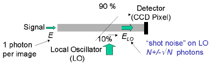
Figure 2: 1 photon equivalent signal (accounting Heterodyne gain), and shot noise on the holographic Local Oscillator beam.

In order to discuss the effect of the shot noise on the heterodyne signal ${\cal E}_{p,q}{\cal E}_{LO}^{*}$ of Eq.II-B, let us consider the simple situation sketched on Fig.2. A weak object field ${{E}}$, with 1 photon or 1 photo electron per pixel and per frame, interferes with a LO field ${{E}}_{LO}$ with $N$ photons, where $N$ is large ($N=10^{4}$, in the case of our experiment). Since the LO beam signal $a^{2}T|{\cal E}_{LO}|^{2}$ is equal to $N$ photons, and the object field signal $a^{2}T|{\cal E}_{p,q}|^{2}$ is one photon, we have:

$$I_{k,p,q}=N+1+i_{k,p,q}+a^{2}T{\cal E}_{p,q}{\cal E}_{LO}^{*}e^{...}+c.c.$$ (17)

Note that the heterodyne signal ${\cal E}_{p,q}{\cal E}_{LO}^{*}$ is much larger than $|{\cal E}_{p,q}|^{2}$. This is the gain effect, associated to the coherent detection of the field ${\cal E}_{p,q}$. This gain is commonly called ”heterodyne gain”, and is proportional to the amplitude of the LO field ${\cal E}_{LO}^{*}$.

The purpose of the present discussion is to determine the effect of the noise term $i_{k,p,q}$ of Eq.17 on the holographic signal $H_{p,q}$. Since $H_{p,q}$ involves only the heterodyne term ${\cal E}_{p,q}{\cal E}_{LO}^{*}$ (see Eq.9), we have to compare, in Eq.17,

• the shot noise term $i_{k,p,q}$.

• and the heterodyne term ${\cal E}_{p,q}{\cal E}_{LO}^{*}$

Let’s consider first the shot noise term. We have

$$\langle i_{k,p,q}^{2}\rangle=\langle I_{k,p,q}\rangle=N+1\simeq N$$ (18)

The variance of the shot noise term is thus $\sqrt{N}=10^{2}$. Since this noise is mainly related to the shot noise on the local oscillator (since $N\gg 1$), one can group together, in Eq.17, the LO beam term (i.e. $N$) with the noise term $i_{k,p,q}$, and consider that the LO beam signal fluctuates, the number of LO beam photons being thus ”$N\pm\sqrt{N}$”, as mentioned on Fig.2.

Consider now the the heterodyne beat signal. Since we have $N$ photons on the LO beam, and 1 photon on the object beam, we get:

$$a^{2}T|{\cal E}_{p,q}{\cal E}_{LO}^{*}|\equiv\left(\left(a^{2}T{|\cal E}_{p,q}|^{2}\right)\left(a^{2}T{|\cal E}_{LO}|^{2}\right)\right)^{1/2}=N^{1/2}$$ (19)

The heterodyne beat signal ${\cal E}_{p,q}{\cal E}_{LO}^{*}$ is thus $\sqrt{N}=10^{2}$.

The shot noise term $i_{k,p,q}$ is thus equal to the heterodyne signal ${\cal E}_{p,q}{\cal E}_{LO}^{*}$ corresponding to 1 photon on the object field. This means that shot noise $i_{k,p,q}$ yields an equivalent noise of 1 photon per pixel, on the object beam. This result is obtained here for 1 frame. We will show that it remains true for a sequence of $4n$ frames, whatever $4n$ is.

III-C The Object field Equivalent Noise for $4n$ frames

Let us introduce the DC component signal $D$, which is similar to the heterodyne signal $H$ given by Eq.8, but without phase factors:

$$D\equiv\sum_{k=0}^{4n-1}I_{k}$$ (20)

The component $D$ can be defined for each pixel $(p,q)$ by :

$$D_{p,q}\equiv\sum_{k=0}^{4n-1}I_{k,p,q}$$ (21)

Since $I_{k,p,q}$ is always large in real life (about $10^{4}$ in our experiment), the shot noise term can be neglected in the calculation of $D_{p,q}$ by Eq.21. We have thus:

$$D_{p,q}\equiv\sum_{k=0}^{4n-1}I_{k,p,q}=4na^{2}T\left(|{\cal E}_{p,q}|^{2}+|{\cal E}_{LO}|^{2}\right)$$ (22)

We are implicitly interested by the low signal situation (i.e. ${\cal E}_{p,q}\ll{\cal E}_{LO}$ ) because we focus on noise analysis. In that case, the $|{\cal E}_{p,q}|^{2}$ term can be neglected in Eq.22. This means that $D_{p,q}$ gives a good approximation for the LO signal.

$$D_{p,q}\equiv\sum_{k=0}^{4n-1}I_{k,p,q}\simeq 4na^{2}T|{\cal E}_{LO}|^{2}$$ (23)

We can get then the signal field $|{\cal E}_{p,q}|^{2}$ from Eq.9 and Eq.23:

$$\frac{|H_{p,q}|^{2}}{D_{p,q}}\simeq 4na^{2}T|{\cal E}_{p,q}|^{2}$$ (24)

In this equation, the ratio ${|H_{p,q}|^{2}}/{D_{p,q}}$ is proportional to the number of frames of the sequence ($4n$), This means that ${|H_{p,q}|^{2}}/{D_{p,q}}$ represents the signal field $|{\cal E}_{p,q}|^{2}$ summed over the all frames.

Let us calculate the effect of the shot noise on ${|H_{p,q}|^{2}}/{D_{p,q}}$. To calculate this effect, one can make a Monte Carlo simulation as mentioned above, but a simpler calculation can be done here. In Eq.24, we develop $|H_{p,q}|$ in statistical average and noise components (as done for $I_{k,p,q}$ in Eq.14), while neglecting noise in $D_{p,q}$.

We get:

$$\left\langle\frac{|H_{p,q}|^{2}}{D_{p,q}}\right\rangle\simeq\frac{1}{\langle D_{p,q}\rangle} \times (|\langle H_{p,q}\rangle|^{2}+\langle|h_{p,q}|^{2}\rangle$$

$$+ \langle\langle H_{p,q}\rangle h_{p,q}^{*}\rangle+\langle\langle H_{p,q}^{*}\rangle h_{p,q})$$

where

$$H_{p,q}=\langle H_{p,q}\rangle+h_{p,q}$$ (26)

with

$$h_{p,q}=\sum_{k=0}^{4n-1}j^{k}i_{k,p,q}$$ (27)

which is the shot noise random contribution to $H_{p,q}$. In Eq.III-C the $\langle\langle H_{p,q}\rangle h_{p,q}^{*}\rangle$ term is zero since $h_{p,q}^{*}$ is random while $\langle H_{p,q}\rangle$ is not random. The two terms $\langle\langle H_{p,q}\rangle h_{p,q}^{*}\rangle$ and $\langle\langle H_{p,q}^{*}\rangle h_{p,q}\rangle$ can be thus removed.

On the other hand, we get for $|h_{p,q}|^{2}$

$$|h_{p,q}|^{2}=\sum_{k=0}^{4n-1}|i_{k,p,q}|^{2}+\sum_{k=0}^{4n-1}\sum_{k^{\prime}=0,k^{\prime}\neq k}^{4n-1}j^{k-k^{\prime}}i_{k,p,q}i_{k^{\prime},p,q}$$ (28)

Since $i_{k,p,q}$ and $i_{k^{\prime},p,q}$ are uncorrelated, the $i_{k,p,q}i_{k^{\prime},p,q}$ terms cancel in the calculation of the statistical average of $|h_{p,q}|^{2}$. We get then from Eq.15

$$\langle|h_{p,q}|^{2}\rangle=\sum_{k=0}^{4n-1}\langle|i_{k,p,q}|^{2}\rangle=\sum_{k=0}^{4n-1}\langle I_{k,p,q}\rangle=\langle D_{p,q}\rangle$$ (29)

and Eq.III-C becomes:

$$\left\langle\frac{|H_{p,q}|^{2}}{D_{p,q}}\right\rangle=\frac{|\langle H_{p,q}\rangle|^{2}}{\langle D_{p,q}\rangle}+1$$ (30)

This equation means that the average detected intensity signal $\langle{|H_{p,q}|^{2}}/{D_{p,q}}\rangle$ is the sum of the square of the average object field $\langle|H_{p,q}|\rangle/\sqrt{\langle D_{p,q}\rangle}$ plus one photo-electron. Without illumination of the object, the average object field is zero, and the detected signal is 1 photo-electron. The equation establishes thus that the LO shot noise yields a signal intensity corresponding exactly 1 photo-electron per pixel whatever the number of frames $4n$ is.

The 1 e noise floor we get here can be also interpreted as resulting from the heterodyne detection of the vacuum field fluctuations [50].

III-D The detection bandwidth, and the noise

From a practical point of view, the holographic detected signal intensity increases linearly with the acquisition time $4nT$ (since ${|H_{p,q}|^{2}}/{D_{p,q}}\propto 4n$), while the noise contribution remains constant: the 1 e noise calculated by Eq.III-C corresponds to a sequence of $4n$ frames, whatever the number $4n$ of frames is. The coherent character of holographic detection explains this paradoxical result.

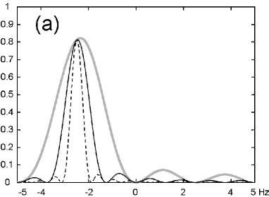
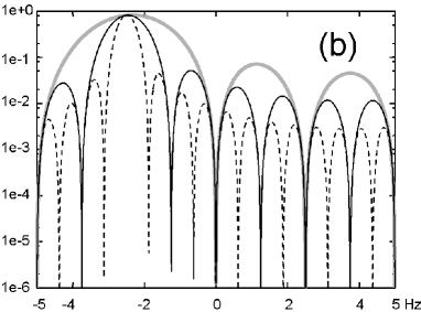
Figure 3: Frequency response $|\eta(x)|^{2}$ for heterodyne signal in intensity, as a function of the heterodyne beat frequency $x=f-f_{LO}$ for sequences of $4n$ frames with $4n=4$ (heavy grey line), $4n=8$ (solid black line), and $4n=16$ (dashed black line). Calculation is done for $T=0.1$ s. Vertical axis axis is $|\eta(x)|^{2}$ in linear (a) and logarithmic (b) scales. Horizontal axis is $x=f-f_{LO}$ in Hz.

The noise remains constant with time because the noise is broadband (it is a white noise), while the detection is narrowband. The noise that is detected is proportional to the product of the exposure time, which is proportional to the acquisition time $4nT$, with the detection Bandwidth, which is inversely proportional to $4nT$. It does not depend thus on $4nT$.

To illustrate this point, we have calculated, as a function of the exposure time $4nT$, the frequency response of the coherent detection made by summing the $4n$ frames with the phase factors $j^{k}$ of Eq.8. Let us call $\eta$ the detection efficiency for the signal field complex amplitude. We get:

$$\eta(x) = \frac{1}{4nT}\sum_{k=0}^{4n-1}j^{k}\int_{t=kT-T/2}^{kT+T/2}e^{j2\pi xt}dt$$ (31)

$$= \textrm{sinc}(\pi xT)\times\frac{1}{4n}\sum_{k=0}^{4n-1}j^{k}{\rm e}^{j2\pi kxT}$$ (32)

Here $x=f-f_{LO}$ is the heterodyne beat frequency; $f$ is the optical frequency of the signal beam, and $f_{LO}$ the frequency of the LO beam. In equation 31, the factor $\textrm{sinc}(\pi xT)$ corresponds to the integration of the beat signal, whose frequency $x$ is non zero, over the CCD frame finite exposure time $T$. The summation over the frames $k$ of Eq.8 yields, in Eq.31, to sum the phase ${\rm e}^{j2\pi kTx}$ of the heterodyne beat at the beginning of each frame $k$ with the phase factor $j^{k}$. To the end, the factor $1/4n$ in Eq.31 is a normalization factor that is the inverse of the number of terms within the summation over $k$. This $1/4n$ factor keeps the maximum of $|\eta(x)|$ slightly lower than 1.

We have calculated, and plotted on Fig.3, the detection frequency spectrum $|\eta(x)|^{2}$ for sequences with different number of frames $4n$. The heavy grey line curve corresponds to 4 frames, the solid line curve to 8 frames, and the dashed line to 16 frames. As seen, the width of the frequency response spectrum (and thus the frequency response area) is inversely proportional to the exposure time ($(4\,T)^{-1}$, $(8\,T)^{-1}$ and $(16\,T)^{-1}$ respectively).

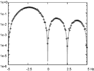
Figure 4: Frequency response for heterodyne signal in intensity, as a function of the heterodyne beat frequency $x=f-f_{LO}$ for a sequence of $4$ frames: theory $|\eta(x)|^{2}$ (heavy grey line), and experiment $W(x)$ (points). Calculation and experiment are done with $T=0.1$ s. Vertical axis axis is $|\eta(x)|^{2}$ or $W(x)$ in logarithmic scales. Horizontal axis is $x=f-f_{LO}$ in Hz.

To verify the validity of Eq.31, we have swept the frequency $f_{LO}=\omega_{LO}/(2\pi)$ of our holographic LO by detuning the AOMs frequency (see Fig.1), while keeping constant the illumination frequency $f$. We have then measured the weight $W(x)$ of the reconstructed holographic intensity signal $H^{2}$ as a function of the beat frequency $x=f-f_{LO}$. Figure 4 shows the comparison of the theoretical signal $|\eta(x)|^{2}$ (heavy grey line), with the experimental data $W(x)$ (points). The agreement is excellent.

IV Reaching the theoretical Shot Noise in experiment

In the previous sections, we have shown that the theoretical noise on the holographic reconstructed intensity images is 1 photo electron per pixel whatever the number of recorded frames is. We will now discuss the ability to reach this limit in real time holographic experiment. Since we consider implicitly a very weak object beam signal, the noises that must be considered are

• the read noise of the CCD camera,

• the quantization noise of the camera A/D converter,

• the technical noise on the LO beam,

• and the LO beam shot noise, which yields the theoretical noise limit.

Number of pixels	1280 (H) $\times$ 1024 (V)
Pixel size	$6.7\times 6.7\mu$m
Frame Rate	12.5 fps
Full Well Capacity	25 000 e
A/D Converter	12 bits: 0… 4095 DC
A/D conversion factor (Gain)	4.8 e/DC
QE $@$ 500 nm :	40 %
QE $@$ 850 nm :	6%
Read Noise	20 e
Dark Noise	3 e/sec/pix

Figure 5: Main characteristics of the PCO Pixelfly Camera

IV-A The technical noise within the $(k_{x},k_{y})$ reciprocal space

The main characteristics of our camera are given in Fig.5. In a typical experiment, the LO beam power is adjusted in order to get $2000$ DC on the A/D Converter, i.e. about $10^{4}$ e on the each CCD pixel. The LO shot noise, which is about 100 e, thus much larger than the Read Noise (20 e), than the Dark Noise (3 e/sec), and than the A/D converter quantization noise (4.8 e, since 1 DC corresponds to 4.8 e). The noise of the camera, which can be neglected, is thus not limiting in reaching the noise theoretical limit.

The LO beam that reaches the camera is essentially flat field (i.e. the field intensity $|{\cal E}_{LO}|^{2}$ is the same for all the pixels). The LO beam technical noise is thus highly correlated from pixel to pixel. This is for example the case of the noise induced by the fluctuations of the main laser intensity, or by the vibrations of the mirrors within the LO beam arm. To illustrate this point, we have recorded a sequence of $4n=4$ frames $I_{k}$ with LO beam, but without signal (i.e. without illumination of the object). We have recorded thus the hologram of the ”vacuum field”. We have calculated then the complex hologram $H$ by Eq.8, and the reciprocal space hologram $\tilde{H}$ by FFT (i.e. by Eq.10).

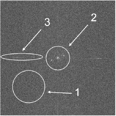
Figure 6: Intensity image of $\tilde{H}(k_{x},k_{y},0)$ for $4n=4$ frames without signal $\cal E$. Three kind of noises can be identified. left : FFT aliasing, down left : shot noise, middle : technical noise of the CCD. By truncating the image and keeping only the left down part, the shot noise limit is reached. The image is displayed in arbitrary logarithm grey scale.

The reciprocal space holographic intensity $|\tilde{H}|^{2}$ is displayed on Fig.6 in arbitrary logarithm grey scale. On most of the reciprocal space (within for example circle 1), $|\tilde{H}|^{2}$ corresponds to a random speckle whose average intensity is uniformly distributed along $k_{x}$ and $k_{y}$. One observes nevertheless bright points within circle 2, which corresponds to $(k_{x},k_{y})\simeq(0,0)$. These points correspond to the technical noise, which is flat field within the CCD plane $(x,y)$, and which has thus a low spatial frequency spread within the $(k_{x},ky)$ reciprocal space. One see also, on the Fig.6 image, an horizontal and a vertical bright line, which corresponds to $k_{y}=0$ and $k_{x}=0$ (zone 3 on Fig.6). These parasitic bright lines are related to Fast Fourier Transform aliases, that are related to the discontinuity of the signal $I_{k}$ and $H$ at edge of the calculation grid, in the $(x,y)$ space.

We have measured $\langle|{\tilde{H}}|^{2}\rangle$ by replacing the statistical average $\langle~{}\rangle$ by a spatial average over a region of the conjugate space without technical noise (i.e. over region 1). This gives a measurement of $\langle|{\tilde{H}}|^{2}\rangle$, i.e. a measurement of $\langle|H|^{2}\rangle$, since the space average of $|{\tilde{H}}|^{2}$ and $|{H}|^{2}$ are equal, because of the FT Parceval theorem. We have also measured $D$ from the sequence of frames $I_{k}$ (see Eq.20). Knowing the A/D conversion factor (4.8 e/DC), we have calculated the noise intensity $\langle|{\tilde{H}}|^{2}\rangle/\langle D\rangle$ in photo-electron units, and we get, within 10%, $1$ photo electron per pixel, as expected theoretically for the shot noise (see Eq.III-C).

This result proves that it is possible to perform shot noise limited holography in actual experiments. Since the low spatial frequency region of the reciprocal space (region 2) must be avoided because of the technical noise, it is necessary to perform digital holography in an off-axis configuration, in order to reach the Eq.III-C shot noise limit.

IV-B Effect the finite size of the pixel.

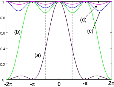
Figure 7: One dimension (1D) angular response of the detection efficiency for the intensity $\sum_{m}|\textrm{sinc}(X+m\pi)|^{2}$ as a function of $X$ for the main lobe: $m=0$ (a); for the main lobe and 2 aliases: $m=0,\pm 1$ (b); for the main lobe and 4 aliases: $m=0,\pm 1,\pm 2$ (c); for the main lobe and 10 aliases: $m=0,\pm 1,\pm 2,...\pm 5$ (d).

Because of the finite size of the pixels $d_{pix}$, the heterodyne detection efficiency within direction $k_{x},k_{y}$ is weighted by a factor $\zeta$ for the field $\tilde{H}$, and $|\zeta|^{2}$ for the intensity $|\tilde{H}|^{2}$ with:

$$\zeta(k_{x},k_{y}) = \frac{1}{d_{pix}^{~{}2}}~{}\int_{x=\frac{-1}{2}d_{pix}}^{\frac{1}{2}d_{pix}}\int_{y=\frac{-1}{2}d_{pix}}^{\frac{1}{2}d_{pix}}e^{j(k_{x}x+k_{y}y)}dx~{}dy$$ (33)

$$= \textrm{sinc}(X)\textrm{sinc}(Y)$$

with $X=k_{x}d_{pix}/2$ and $Y=k_{y}d_{pix}/2$. This factor $\zeta$ corresponds to the angular sinc diffraction pattern of the rectangular pixels, which affects the component of $\tilde{H}$ corresponding to the signal of the object. The efficiency in energy $|\zeta|^{2}$ is plotted in Fig.7, curve (a) in black.

Because of the sampling made by the CCD pixels, the hologram $\tilde{H}(k_{x},k_{y})$ is periodic in the reciprocal space, with a periodicity equal to $2\pi/d_{pix}$ for $k_{x}$ and $k_{y}$, or $\pi$ for $X$ and $Y$. This means that the edges of the FFT calculation grid, which are displayed on Fig.7 as vertical dashed lines, corresponds to $k_{x},k_{y}=\pm\pi/d_{pix}$ or to $X,Y=\pm\pi/2$. Note that the detection efficiency is non zero at the edges of the calculation grid since we have $|\zeta|^{2}=4/\pi^{2}\simeq 0.40$ for $X=\pi/2$ and $Y=0$.

If the factor $|\zeta|^{2}$ affects the component of $|\tilde{H}|^{2}$ corresponding to the signal of the object, it do not affects the shot noise component, whose weight is 1 whatever $k_{x}$ and $k_{y}$ are. One can demonstrate this result by calculating the noise by Monte Carlo simulation from Eq.14 and Eq.16. The Monte Carlo simulation yields a fully random speckle noise, both in the $x,y$ space, and in the $k_{x},k_{y}$ reciprocal space.

This point can be understood another way, which is illustrated by Fig.7. Each pixel is a coherent detector, whose detection antenna diagram is the Fig.7 (a) sinc function. Because of the periodicity within the reciprocal space, the signal that is detected for $(k_{x},k_{y})$ or for $(X,Y)$ corresponds to the sum of the signal within the main lobe $(X,Y)$, and within all the aliases corresponding to the periodicity $(X+m\pi,Y+m^{\prime}\pi)$. Since the object is located within a well defined direction, the main lobe contribute nearly alone for the signal. But this is not true for the shot noise, since the shot noise (or the vacuum field noise) spreads over all $(k_{x},k_{y})$ points of the reciprocal space with a flat average density. One has thus to sum the response of the main lobe (i.e. $|\textrm{sinc}(X)|^{2}$ in 1D) with all the periodicity aliases (i.e. $|\textrm{sinc}(X+m\pi)|^{2}$ with $m\neq 0$). Fig.7 shows the 1D angular response $\sum_{m}|\textrm{sinc}(X+m\pi)|^{2}$ that correspond to sum of the main lobe with more and more aliases. As seen, adding more and more aliases make the angular response flat and equal to one.

IV-C Experimental validation with an USAF target.

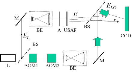
Figure 8: Setup of the test experiment with USAF target. L: main laser; BS: Beam splitter; AOM1 and AOM2: acousto optic modulators; BE: beam expander; M: mirror; A1 and A2: light attenuators. USAF: transmission USAF target that is imaged. CCD : CCD camera.

We have verified that it is possible to perform shot noise limited holography in actual experiments, by recording the hologram of an USAF target in transmission. The holographic setup is sketched on Fig.8. We have recorded sequences of $4n=12$ frames, and we have reconstructed the image of the USAF target.

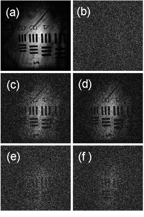
Figure 9: (a,c,d): Reconstructions of an USAF target with different level of illumination 700 (a), 1 (c) and 0.15 e/pixel (d). (b): Simulated Shot Noise noise image. (e,f): Simulated reconstructed image obtained by mixing image (a) with weight $X$, and image (b) with weight $1-X$. The weight $X$ is $1/700$ (e), and $0.15/700$ (f). Images are displayed in arbitrary logarithmic grey scale.

Figure 9 shows the holographic reconstructed images of the USAF target. The intensity of the signal illumination is adjusted with neutral density filters. In order to filter off the technical noise, the reconstruction is done by selecting the order 1 image of the object, within the reciprocal space [8]. Since the $400\times 400$ pixels region that is selected is off axis, the low spatial frequency noisy region, which corresponds to the zero order image (region 1 on Fig.6), is filtered-off.

Figure 9 (a,c,d) shows the reconstructed images obtained for different USAF target illumination levels. For each image, we have measured the average number of photo electrons per pixel corresponding to the object beam, within the reciprocal space region that has been selected for the reconstruction (i.e. $400\times 400$ pixels). The images of Fig. 9 correspond to 700 (a), 1 (c), and 0.15 e/pix (d) respectively. The object beam intensity has been measured by the following way. We have first calibrated the response of our camera with an attenuated laser whose power is known. We have then measured with the camera, at high level of signal, the intensity of the signal beam alone (without LO beam). We have decreased, to the end, the signal beam intensity by using calibrated attenuator in order to reach the low signal level of the images of Fig. 6 (a,c,d). In the case of image (a) with 700e/pix, we also have measured the averaged signal intensity from the data by calculating $|H|^{2}/D$ (see Eq.24). The two measurements gave the same result: 700e per pixel.

On figure 9 (a), with 700e per pixel, the USAF signal is much larger than the shot noise, and the Sinal to Noise Ratio (SNR) is large. On figure 9 (c), with 1 e per pixel, the USAF signal is roughly equal to the shot noise, and the SNR is about 1. With 0.15e per pixel, the SNR is low on Fig.9 (d) (about 0.15), and the USAF is hardly seen. It is nevertheless quite difficult to evaluate the SNR of an image. To perform a more quantitative analysis of the noise within the images, we have synthesized noisy images of 9 (e,f) by adding noise to the Fig. 9 (a) noiseless image. We have first synthesized a pure Shot Noise image , which corresponds to the image that is expected without signal.

The Shot Noise, which is displayed on Fig.9 (b), is obtained by the following way. From one of the measured frames (for example $I_{0}$) we have calculated the noise components $i_{k,p,q}$ by Monte Carlo drawing with the condition:

$$\langle i_{k,p,q}^{2}\rangle=I_{0,p,q}$$ (34)

This condition corresponds to Eq.15 since $\langle I_{k,p,q}\rangle\simeq I_{0,p,q}$. We have then synthesize the sequence of image $I_{k}$ by:

$$I_{k,p,q}=I_{0,p,q}+i_{k,p,q}$$ (35)

The Shot Noise image of Fig.9 (b) is reconstructed then from the $I_{k,p,q}$ sequence.

Image	Signal (e/pix)	Noise (e/pix)
a	$700$	1
b	0	1
c	$1$	1
d	$0.15$	1
e	$1$	1
f	$0.15$	1

Figure 10: Signal and shot Noise on Images of Fig.9

We have synthesized noisy images by summing the noiseless image of Fig.9 (a) with weight $X$, with the Shot Noise image of Fig.9 (b) with weight $(1-X)$. The image of Fig. 9 (e) is obtained with $X=1/700$. As shown on the table of Fig.10, Fig. 9 (e) corresponds to the same signal, and the same noise than Figure 9 (c) (1e of signal, and 1e of noise respectively). Fig. 9 (c) and Fig. 9 (e), which have been displayed here with the same linear grey scale, are visually very similar and exhibit the same SNR. The image of Fig. 9 is similarly obtained with $X=0.15/700$. It corresponds to the same Signal and Noise than Figure 9 (d) (0.15e of signal, and 1e of noise), and, as expected, Fig. 9 (d) and Fig. 9 (f), which have been displayed here with the same linear grey scale, are similar and exhibit the same SNR too.

Here we demonstrated our ability to synthesize a noisy image with a noise that is calculated by Monte Carlo from Eq.34 and 35. Moreover, we have verified that the noisy image is visually equivalent to the image we have obtained in experiments. These results prove that we are able to quantitatively account theoretically the noise, and that the noise that is obtained in experiments reaches the theoretical limit.

V Conclusion

In this paper we have studied the noise limits in digital holography. We have shown that in high heterodyne gain of the holographic detection (achieved when the object field power is much weaker than the LO field power), the noise of the CCD camera can be neglected. Moreover by a proper arrangement of the holographic setup, that combines off-axis geometry with phase shifting acquisition of holograms, it is possible to reach the theoretical shot noise limit. We have studied theoretically this limit, and we have shown that it corresponds to 1 photo electron per pixel for the whole sequence of frame that is used to reconstruct the holographic image. This paradoxical result is related to the heterodyne detection, where the detection bandwidth is inversely proportional to the measurement time. We have verified all our results experimentally, and we have shown that is possible to image an object at very low illumination levels. We have also shown that is possible to mimic the very weak illumination levels holograms obtained in experiments by Monte Carlo noise modeling. This opens the way to simulation of ”gedanken” holographic experiments in weak signal conditions.

Frédéric Verpillat Frédéric Verpillat entered the Ecole Normale Supérieure of Lyon (France) in 2005, then obtained the M.S degree of the Ecole Polytechnique Fédérale of Lausanne (Switzerland) in microengineering in 2009. His specialization is applied optics for biology or medicine (microscopy, optical tomography). He’s preparing a PhD degree at the Laboratoire Kastler Brossel under the direction of Dr. Michel Gross on the tracking of Nanoparticles with digital holography.

Fadwa Joud Fadwa Joud holds an M.S degree in Condensed Matter and Radiation Physics from Université Joseph Fourrier Grenoble 1, France. Passionate with NanoBiophotonics, she joined, in October 2008, the team Optics and Nano Objects at the Laboratoire Kastler Brossel of the École Normale Supérieure in Paris - France to prepare a PhD degree in applied physics under the supervision of Dr. Michel Gross. Her major research project is Holographic Microscopy and its applications in the field of Biology and the detection of Nanoparticles.

Michael Atlan Michael Atlan is a research investigator at CNRS. He studied to deepen expertise in optical physics during his PhD and postdocs under the tutelage of Drs. Claude Boccara, Andrew Dunn, Maite Coppey and Michel Gross. He works on non-invasive and non-ionizing imaging modalities to assess biological structures and dynamic processes from subcellular to tissular scales, designing coherent optical detection schemes to enable highly sensitive imaging at high throughput.

Michel Gross Michel Gross enter the French Ecole Normale Supérieure in 1971. He joined the Laboratoire Kastler Brossel (Paris) in 1975, where he is research scientist. He receive his Ph.D from University Pierre et Marie Curie, Paris, France in 1980. His scientific interests are atomic physics (superradiance, Rydberg and circular atoms), excimer laser refractive surgery, millimeter wave and teraherz technology, and digital. He developed a Millimeter Wave Network Analyzer and participate to the creation the AB Millimeter company. His main current interest is digital holography. He has published about 80 scientific papers, and is co-inventor of 6 patents.

References

- [1] D. Gabor, “Microscopy by reconstructed wavefronts,” Proc. R. Soc. A, vol. 197, p. 454, 1949.
- [2] A. Macovsky, “Consideration of television holography,” Optica Acta, vol. 22, no. 16, p. 1268, August 1971.
- [3] U. Schnars, “Direct phase determination in hologram interferometry with use of digitally recorded holograms,” JOSA A., vol. 11, p. 977, July 1994.
- [4] J. W. Goodmann and R. W. Lawrence, “Digital image formation from electronically detected holograms,” Appl. Phys. Lett., vol. 11, p. 77, 1967.
- [5] E. Leith, J. Upatnieks, and K. Haines, “Microscopy by wavefront reconstruction,” Journal of the Optical Society of America, vol. 55, no. 8, pp. 981–986, 1965.
- [6] U. Schnars and W. Jüptner, “Direct recording of holograms by a CCD target and numerical reconstruction,” Appl. Opt., vol. 33, no. 2, pp. 179–181, 1994.
- [7] T. M. Kreis, W. P. O. Juptner, and J. Geldmacher, “Principles of digital holographic interferometry,” SPIE, vol. 3478, p. 45, July 1988.
- [8] E. Cuche, P. Marquet, and C. Depeursinge, “spatial filtering for zero-order and twin-image elimination in digital off-axis holography,” Appl. Opt., vol. 39, no. 23, pp. 4070–4075, 2000.
- [9] I. Yamaguchi and T. Zhang, “Phase-shifting digital holography,” Optics Letters, vol. 18, no. 1, p. 31, 1997.
- [10] U. Schnars and W. Juptner, “Digital recording and numerical reconstruction of holograms,” Measurement science and technology, vol. 13, no. 9, pp. 85–101, 2002.
- [11] A.-F. Doval, “A systematic approach to tv holography.” Measurement-Science and Technology., vol. 11, p. 36, January 2000.
- [12] Y. Pu and H. Meng, “Intrinsic speckle noise in off-axis particle holography,” Journal of the Optical Society of America A, vol. 21, no. 7, pp. 1221–1230, 2004.
- [13] T. Colomb, P. Dahlgren, D. Beghuin, E. Cuche, P. Marquet, and C. Depeursinge, “Polarization imaging by use of digital holography,” Applied optics, vol. 41, no. 1, pp. 27–37, 2002.
- [14] E. Cuche, F. Belivacqua, and C. Depeursinge, “Digital holography for quantitative phase-contrast imaging,” Opt. Lett., vol. 24, no. 5, pp. 291–293, 1999.
- [15] J. Massig, “Digital off-axis holography with a synthetic aperture,” Optics letters, vol. 27, no. 24, pp. 2179–2181, 2002.
- [16] Z. Ansari, Y. Gu, M. Tziraki, R. Jones, P. French, D. Nolte, and M. Melloch, “Elimination of beam walk-off in low-coherence off-axis photorefractive holography,” Optics Letters, vol. 26, no. 6, pp. 334–336, 2001.
- [17] P. Massatsch, F. Charrière, E. Cuche, P. Marquet, and C. Depeursinge, “Time-domain optical coherence tomography with digital holographic microscopy,” Applied optics, vol. 44, no. 10, pp. 1806–1812, 2005.
- [18] E. Absil, G. Tessier, M. Gross, M. Atlan, N. Warnasooriya, S. Suck, M. Coppey-Moisan, and D. Fournier, “Photothermal heterodyne holography of gold nanoparticles,” Opt. Express, vol. 18, pp. 780–786, 2010.
- [19] P. Marquet, B. Rappaz, P. Magistretti, E. Cuche, Y. Emery, T. Colomb, and C. Depeursinge, “Digital holographic microscopy: a noninvasive contrast imaging technique allowing quantitative visualization of living cells with subwavelength axial accuracy,” Optics letters, vol. 30, no. 5, pp. 468–470, 2005.
- [20] M. Atlan, M. Gross, P. Desbiolles, É. Absil, G. Tessier, and M. Coppey-Moisan, “Heterodyne holographic microscopy of gold particles,” Optics Letters, vol. 33, no. 5, pp. 500–502, 2008.
- [21] T. Zhang and I. Yamaguchi, “Three-dimensional microscopy with phase-shifting digital holography,” Optics letters, vol. 23, no. 15, pp. 1221–1223, 1998.
- [22] T. Nomura, B. Javidi, S. Murata, E. Nitanai, and T. Numata, “Polarization imaging of a 3D object by use of on-axis phase-shifting digital holography,” Optics letters, vol. 32, no. 5, pp. 481–483, 2007.
- [23] I. Yamaguchi, T. Matsumura, and J. Kato, “Phase-shifting color digital holography,” Optics letters, vol. 27, no. 13, pp. 1108–1110, 2002.
- [24] F. Le Clerc, M. Gross, and L. Collot, “Synthetic-aperture experiment in the visible with on-axis digital heterodyne holography,” Optics Letters, vol. 26, no. 20, pp. 1550–1552, 2001.
- [25] S. Tamano, Y. Hayasaki, and N. Nishida, “Phase-shifting digital holography with a low-coherence light source for reconstruction of a digital relief object hidden behind a light-scattering medium,” Applied optics, vol. 45, no. 5, pp. 953–959, 2006.
- [26] I. Yamaguchi, T. Ida, M. Yokota, and K. Yamashita, “Surface shape measurement by phase-shifting digital holography with a wavelength shift,” Applied optics, vol. 45, no. 29, pp. 7610–7616, 2006.
- [27] I. Yamaguchi, J. Kato, S. Ohta, and J. Mizuno, “Image formation in phase-shifting digital holography and applications to microscopy,” Applied Optics, vol. 40, no. 34, pp. 6177–6186, 2001.
- [28] F. LeClerc, L. Collot, and M. Gross, “Numerical heterodyne holography using 2d photo-detector arrays,” Optics Letters, vol. 25, p. 716, Mai 2000.
- [29] M. Atlan, M. Gross, and E. Absil, “Accurate phase-shifting digital interferometry,” Optics letters, vol. 32, no. 11, pp. 1456–1458, 2007.
- [30] M. Gross and M. Atlan, “Digital holography with ultimate sensitivity,” Optics Letters, vol. 32, no. 8, pp. 909–911, 2007.
- [31] E. Cuche, P. Marquet, C. Depeursinge et al., “Spatial filtering for zero-order and twin-image elimination in digital off-axis holography,” Applied Optics, vol. 39, no. 23, pp. 4070–4075, 2000.
- [32] M. Gross, M. Atlan, and E. Absil, “Noise and aliases in off-axis and phase-shifting holography,” Applied Optics, vol. 47, no. 11, pp. 1757–1766, 2008.
- [33] F. Joud, F. Laloe, M. Atlan, J. Hare, and M. Gross, “Imaging a vibrating object by Sideband Digital Holography,” Optics Express, vol. 17, p. 2774, 2009.
-
[34]
F. Joud, F. Verpillat, F. Lalo
”e, M. Atlan, J. Hare, and M. Gross, “Fringe-free holographic measurements of large-amplitude vibrations,” Optics Letters, vol. 34, no. 23, pp. 3698–3700, 2009. - [35] M. Atlan, M. Gross, and J. Leng, “Laser Doppler imaging of microflow,” J. Eur. Opt. Soc. Rapid Publications, vol. 1, pp. 06 025–1, 2006.
- [36] M. Atlan, M. Gross, B. Forget, T. Vitalis, A. Rancillac, and A. Dunn, “Frequency-domain wide-field laser Doppler in vivo imaging,” Optics letters, vol. 31, no. 18, pp. 2762–2764, 2006.
- [37] M. Atlan, B. Forget, A. Boccara, T. Vitalis, A. Rancillac, A. Dunn, and M. Gross, “Cortical blood flow assessment with frequency-domain laser Doppler microscopy,” Journal of Biomedical Optics, vol. 12, p. 024019, 2007.
- [38] M. Atlan, M. Gross, T. Vitalis, A. Rancillac, J. Rossier, and A. Boccara, “High-speed wave-mixing laser Doppler imaging in vivo,” Optics Letters, vol. 33, no. 8, pp. 842–844, 2008.
- [39] M. Gross, P. Goy, B. Forget, M. Atlan, F. Ramaz, A. Boccara, and A. Dunn, “Heterodyne detection of multiply scattered monochromatic light with a multipixel detector,” Optics letters, vol. 30, no. 11, pp. 1357–1359, 2005.
- [40] M. Lesaffre, M. Atlan, and M. Gross, “Effect of the Photon’s Brownian Doppler Shift on the Weak-Localization Coherent-Backscattering Cone,” Physical review letters, vol. 97, no. 3, p. 33901, 2006.
- [41] M. Gross, P. Goy, and M. Al-Koussa, “Shot-noise detection of ultrasound-tagged photons in ultrasound-modulated optical imaging,” Opt. Lett., vol. 28, no. 24, pp. 2482–2484, 2003.
- [42] M. Atlan, B. Forget, F. Ramaz, A. Boccara, and M. Gross, “Pulsed acousto-optic imaging in dynamic scattering media with heterodyne parallel speckle detection,” Optics letters, vol. 30, no. 11, pp. 1360–1362, 2005.
- [43] L. Wang and X. Zhao, “Ultrasound-modulated optical tomography of absorbing objects buried in dense tissue-simulating turbid media,” Applied optics, vol. 36, no. 28, pp. 7277–7282, 1997.
- [44] F. Ramaz, B. Forget, M. Atlan, A. Boccara, M. Gross, P. Delaye, and G. Roosen, “Photorefractive detection of tagged photons in ultrasound modulated optical tomography of thick biological tissues,” Optics Express, vol. 12, pp. 5469–5474, 2004.
- [45] L. Wang and G. Ku, “Frequency-swept ultrasound-modulated optical tomography of scattering media,” Optics letters, vol. 23, no. 12, pp. 975–977, 1998.
- [46] M. Gross, F. Ramaz, B. Forget, M. Atlan, A. Boccara, P. Delaye, and G. Roosen, “Theoretical description of the photorefractive detection of the ultrasound modulated photons in scattering media,” Optics Express, vol. 13, pp. 7097–7112, 2005.
- [47] L. Sui, R. Roy, C. DiMarzio, and T. Murray, “Imaging in diffuse media with pulsed-ultrasound-modulated light and the photorefractive effect,” Applied optics, vol. 44, no. 19, pp. 4041–4048, 2005.
- [48] M. Lesaffre, F. Jean, F. Ramaz, A. Boccara, M. Gross, P. Delaye, and G. Roosen, “In situ monitoring of the photorefractive response time in a self-adaptive wavefront holography setup developed for acousto-optic imaging,” Optics Express, vol. 15, no. 3, pp. 1030–1042, 2007.
- [49] L. Yu and M. Kim, “Wavelength-scanning digital interference holography for tomographic three-dimensional imaging by use of the angular spectrum method,” Optics letters, vol. 30, no. 16, pp. 2092–2094, 2005.
- [50] H. Bachor, T. Ralph, S. Lucia, and T. Ralph, A guide to experiments in quantum optics. wiley-vch, 1998.