Circular, stationary profiles emerging in unidirectional abrasion

Abstract

We describe a PDE model of bedrock abrasion by impact of moving particles and show that by assuming unidirectional impacts the modification of a geometrical PDE due to Bloore [7] exhibits circular arcs as solitary profiles. We demonstrate the existence and stability of these stationary, travelling shapes by numerical experiments based on finite difference approximations. Our simulations show that ,depending on initial profile shape and other parameters, these circular profiles may evolve via long transients which, in a geological setting, may appear as non-circular stationary profiles.

1 Introduction

1.1 Motivation and references

Bedrock abrasion by impact of moving particles is a dominant process shaping obstacles in river channels [1]. Abrasion is mostly due to saltating particles, a broad description of their mechanistic properties is presented in [2]. Our goal is to identify and predict the geometry of obstacle profiles created by this process. In a recent paper, a discrete random model describing bedrock profile abrasion was developed and its predictions compared with experiment [3]. The main observation was that stationary profiles emerged both in the laboratory experiments and the matching discrete simulations. This phenomenon has also been observed in Nature [4],[5],[9]. The aim of the present paper is to present a simple partial differential equation capturing the essence of the physical process and investigate whether it admits stable travelling front solutions which are compatible with the numerical and experimental results obtained in [3] and observed in [4],[5].

1.2 Basic assumptions and notations

If $(x,y,z)$ are Cartesian coordinates we take $y$ along the vertical direction. We assume, for simplicity, that the system is uniform in the horizontal direction perpendicular the direction of motion of the abrading particles. Thus the bedrock profile starts off and remains independent of the $z$ coordinate and is therefore given by a single function $y=y(x,t)$ of space and time. The tangent to the profile makes an angle $\psi$ with respect to the horizontal, so the inward normal to the profile makes an angle $\psi-\frac{\pi}{2}$ with the horizontal. We also introduce

$$y^{\prime}=\partial y/\partial x=\tan\psi$$ (1)

and assume, following [3], that

• small abraders are incident from the left making an angle $\phi$ with the horizontal.

• the angle of the colliding face of large abraders is uniformly distributed between $0$ and $\frac{\pi}{2}$, i.e. the non-uniform flight of abraders does not change this term.

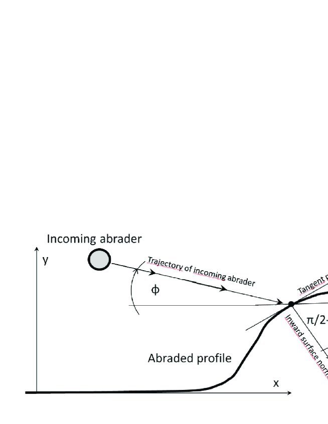
Figure 1: Basic notations

As time proceeds, a point on the profile with constant $x$ coordinate moves with vertical velocity given by

$$v_{\rm vertical}=\frac{\partial y}{\partial t}=\dot{y},$$ (2)

the partial derivative being taken at fixed $x$. The velocity of the same point along the inward normal is:

$$v_{n}=-\dot{y}\cos\psi.$$ (3)

Abrasion due to collisions with incoming abraders with isotropic, uniform distribution has been first derived by Bloore [7], for the detailed derivation of the planar case see also [6]. Under the assumption of unidirectional abraders, Bloore’s PDE can be readily modified by the inclination factor to obtain

$$v_{n}=(v+b\rho)\sin(\psi-\phi),$$ (4)

where $\rho=-y^{\prime\prime}(1+y^{\prime 2})^{-3/2}$ is the geometric curvature and $v,b$ are positive constants. Using the latter expression as well as (3), we obtain

$$-\dot{y}\cos\psi=(v+b\rho)\sin(\psi-\phi)=(v+b\rho)(\sin\psi\cos\phi-\cos\psi\sin\phi)$$ (5)

Using (1), from (5) we obtain

$$-\dot{y}=(v+b\rho)(\cos\phi y^{\prime}-\sin\phi).$$ (6)

Without restricting generality, we assume $\phi=0$ (i.e. that the $x$ axis is aligned with the flight direction of the abraders) to obtain

$$-\dot{y}=y^{\prime}(v+b\rho)=y^{\prime}(v+by^{\prime\prime}(1+y^{\prime 2})^{-\frac{3}{2}}).$$ (7)

Note that $L=b/v$ is the only independent length scale of the equation. Rather than descibe the profile in terms of $y$ considered as a function of $x$ and $t$ we may regard $x$ as a function of $y$ and $t$: $x=x(y,t)$, so we obtain:

$$\dot{x}=(v+b\rho)=(v+bx^{\prime\prime}(1+x^{\prime 2})^{-\frac{3}{2}})\,$$ (8)

where now $\dot{x}=\partial_{t}x(y,t)$ keeping $y$ fixed and $x^{\prime}=\partial_{y}(y,t),$ keeping $t$ fixed.

Our equation is a model of collision-based abrasion, and the first (constant) term corresponds to the abrasion caused by small abrading particles whereas the second (curvature) term is significant if the abrader is large (cf. [7],[3],[6]). Based on this physical background, in forthcoming numerical simulations we will assume that on non-convex parts of the profile the curvature term vanishes (as large abraders are not likely to hit concave domains). Accordingly, the modified equation reads:

$$-\dot{y}=y^{\prime}(v+b\bar{\rho}),\mbox{ where}\quad\bar{\rho}=\rho\mbox{ if }\rho>0\quad\mbox{and}\quad\bar{\rho}=0\mbox{ if }\rho\leq 0.$$ (9)

2 Existence of travelling waves

Note that (7) is first order in time and second order in space and translationally invariant in time. It is also invariant under translations in space, both vertical and horizontal. Being first order in time (7) defines a “flow” on the infinite dimensional space of profiles such that if we are given a smooth initial profile $y(x,0)=y_{\rm initial}(x)$ say, then, at least for some finite time $y(x,t)$ is uniquely determined. In what follows we shall investigate whether, for smooth initial Cauchy data such that $y_{\rm initial}(x)$ is monotonic increasing and tends rapidly to constant values for large negative and positive values of $x$, that the solution $y(x,t)$ ultimately tends to an exact travelling front solution. If it does, then we shall derive the form it must take. If we make the common travelling wave ansatz

$$y=f(x-ct)$$ (10)

and after substituting into (7) solve the resulting ordinary differential equation for $f(s)$ we find that the solutions are all of the form of portions of circles or straight lines which move to the right with speed

$$c=v+\frac{b}{a}$$ (11)

where $a$ is the radius of the circle. Two special cases should be mentioned: For straight lines of course we have $a=\infty$ and $c=v$. In case of $b=0$ we have

$$\frac{\partial y}{\partial t}=-v\frac{\partial y}{\partial x}$$ (12)

whose general solution is

$$y=f(x-ct)\,,\qquad{\rm with}\qquad c=v$$ (13)

thus if $b=0$ then any initial shape moves with to the right with speed $c=v$. These (local) travelling wave solutions travelling with speed given in (11) may easily be derived from the alternative form of the governing equation (8) by making the ansatz $x(y,t)=ct+x(y).$

The local solutions, made up of circles and straight lines may be patched together to give global solutions satisfying the boundary conditions. Matching conditions should be observed carefully. E.g. only segments with identical curvature may be patched together, otherwise the propagation speed $c$ will suffer a jump. If we use boundary conditions representing a ’cliff (cf Figure 1) then we have two options:

• (a) We satisfy horizontal tangency as boundary condition at both lower and upper end. In this case if we apply (9) prescribing that the curvature term vanishes on concave parts. In this case there is no exact travelling wave solutions as the two ends of the cliff can not be joined by a curve with constant curvature. The only exact solutions are half circles, however these contours are not a feasible representation of real cliffs.

• (b) We satisfy the horizontal tangency only at the upper end. At the lower end we do not prescribe a boundary condition, i.e. we essentially cut off the profile at $y=0$. This admits a one-parameter ($R$) family circular arcs which would be exact travelling solutions. This approach could be justified by considering that a vertex on the upper end is convex (thus it will be abraded by large abraders) whereas a vertex on the lower end is concave so large abraders to not smear it out. Small abraders, corresponding to the constant (Eikonal ) term do not abrade any vertices’s. So, admitting a concave vertex at the lower end does not seem to contradict the physical assumptions. This type of boundary condition has been implemented numerically. Figure 2 shows the evolution of a circular arc under (7) and boundary condition (b). The numerical simulation was based on a standard finite difference scheme and we can observe that the circular arc remains invariant and moves by uniform translation.

  

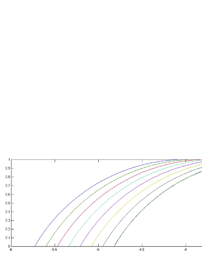
  Figure 2: Circular arc with radius $a=2$ and horizontal tangent at $y=1$ evolving under (7) with $L=b/v=0.6$. Numerical simulation by standard finite difference scheme, using $N_{s}=300$ spatial subdivisions and $\Delta t=10^{-5}$ timestep, profiles plotted after $N_{t}=10^{4}$ timesteps each. Observe that the profile moves with uniform translation, circular arc remains invariant under (7).

3 Stability

Next we investigate the stability of travelling waves. After finding analytical evidence in subsection 3.1 for their local stability we run numerical simulation in subsection 3.2 to test their global attractivity.

3.1 Linear stability: analytical results

Suppose $y(x,t)$ is a solution of (7) when we assume the profile is convex, i.e. $\frac{\partial^{2}y}{\partial x^{2}}$ is negative, so that

$$\frac{\partial y}{\partial t}=-(v-b\frac{\frac{\partial^{2}y}{\partial x^{2}}}{\Bigl{(}1+(\frac{\partial y}{\partial x})^{2}\bigr{)}^{\frac{3}{2}}})\frac{\partial y}{\partial x}$$ (14)

with $b>0$. We consider a nearby solution $y(x,t)+\epsilon(x,t)$ and substitute into (14) and expand to lowest order in $\epsilon$ we get

$$\frac{\partial\epsilon}{\partial t}=-\Bigl{\{}v-b\frac{\frac{\partial^{2}y}{\partial x^{2}}(1-2(\frac{\partial y}{\partial x})^{2}}{\bigl{(}1+(\frac{\partial y}{\partial x})^{2}\bigr{)}^{\frac{5}{2}}}\Bigr{\}}\frac{\partial\epsilon}{\partial x}+b\frac{\partial y}{\partial x}\frac{1}{\bigl{(}1+(\frac{\partial y}{\partial x})^{2}\bigr{)}^{\frac{3}{2}}}\frac{\partial^{2}\epsilon}{\partial x^{2}}$$ (15)

This equation is of the form

$$\frac{\partial\epsilon}{\partial t}+u(x,t)\frac{\partial\epsilon}{\partial x}=\kappa(x,t)\frac{\partial^{2}\epsilon}{\partial x^{2}}$$ (16)

with convection velocity

$$u(x,t)=v-b\frac{\frac{\partial^{2}y}{\partial x^{2}}(1-2(\frac{\partial y}{\partial x})^{2}}{\bigl{(}1+(\frac{\partial y}{\partial x})^{2}\bigr{)}^{\frac{5}{2}}}$$ (17)

and diffusivity

$$\kappa(x,t)=b\frac{\partial y}{\partial x}\frac{1}{\bigl{(}1+(\frac{\partial y}{\partial x})^{2}\bigr{)}^{\frac{3}{2}}}.$$ (18)

Essentially, the first term convects the disturbances with a positive space and time dependent speed $u(x,t)$ and the second term is a diffusion term which causes the disturbance to spread out and decrease in amplitude. This is independent of the particular profile $y(x,t)$. In case of straight lines

$$y=A(x-vt)=As,$$ (19)

based on (17) and (18) we find the convection velocity and diffusivity

$$u(x,t)=v,\qquad\kappa(x,t)=b\frac{A}{1+A^{2}}.$$ (20)

We can aslo rewrite (16) using or using the co-moving variables $s,t$

$$\frac{\partial\epsilon}{\partial t}=b\frac{A}{1+A^{2}}\frac{\partial^{2}\epsilon}{\partial s^{2}}$$ (21)

which is the standard diffusion equation. So we can conclude that all travelling profiles are locally stable, moreover, for straight lines we have explicitly determined the diffusion and convection terms.

3.2 Nonlinear stability: numerical results

Circular profiles are of key interest from the point of view of geological applications, we investigate their stability numerically. Figure 2 illustrated the local stability of circular arcs: by taking such an initial condition the circualr shape was preserved by the PDE. In te next step we consider the convex profile

$$y_{\rm initial}(x)=\tanh(\lambda x),\quad x\geq 0$$ (22)

which satisfy $y(0)=0,\quad y(\infty)=1$ and we evolve these profile numerically considering the boundary condition (b) described in Section 2. The results are shown in Figure 3 and we can observe how the initial profile approaches a circular arc. For better comparison the last profile is plotted next to an exact circle.

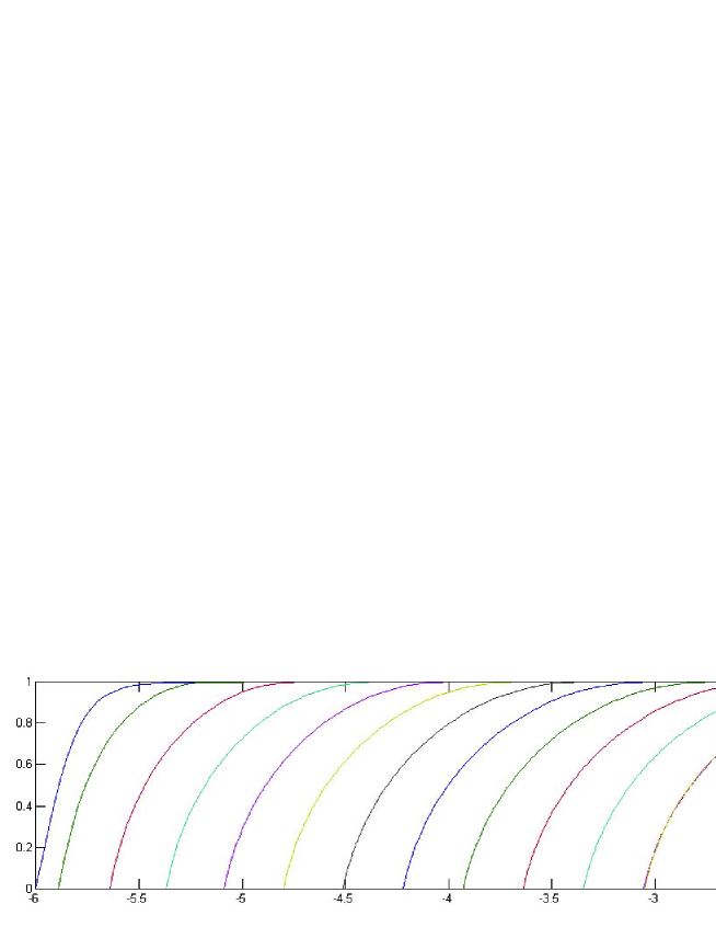
Figure 3: Initial profile given in (22) with $\lambda=5$ evolving under (7) with $L=b/v=0.6$. Numerical simulation by standard finite difference scheme, using $N_{s}=135$ spatial subdivisions and $\Delta t=10^{-5}$ timestep, profiles plotted after $N_{t}=2*10^{4}$ timesteps each (Since the shape changes faster initially, between the first an second profile an intermediate stage at 10.000 steps was inserted). Observe that profile approaches circular arc, next to last profile exact circle is plotted for better comparison.

4 Comparison to experimental data

Here we rely on laboratory experimental data obtained by Wilson [4] [8] using an annular, recirculating flume [8]. In an experiment with this flume [4], single cuboid marble blocks, 10,0 cm tall and 20 cm long, and spanning the 26 cm width of the flume, were fixed on the channel base as a flow obstruction. In our model this would correspond to a Heaviside step function as initial profile shape. The flume was loaded with sorted limestone pebbles to act as bedload abrasion tools, while water discharge was held constant to produce a flow speed of  3ms-1. Under these flow conditions, the limestone pebbles moved by rolling and low saltations in a layer of one to two grain diameters depth along the flume base. Particles moved up the stoss (upstream facing) surface of an obstacle in one or several short hops, and launched off this face clearing the remainder of the obstacle. Resultant erosion of bedrock obstacles was measured using three dimensional laser scanning at intervals throughout experiment runs that lasted 400-690 minutes. Abrasion of obstacles was dominantly on the stoss surface whose initially square cross section evolved to an unpstream facing, almost convex surface. The lower 18.5 mm of the stoss surface were prone to edge chipping, and have been eliminated from consideration, the plotted profile is 81.5mm high. Rates of horizontal erosion were peaking near the top of the obstruction, and decreasing systematically towards the base, resulting in progressive reclining and convex-up rounding of the stoss side. Over time horizontal erosion converged to a common rate at all heights above the flume base, thus, the obstacle stoss faces achieved a time-independent form that advanced downstream into the obstacle. These attributes are shared with bedrock obstacles in the Liwu River, Taiwan, that have been studied extensively [10]. We have set up numerical simulation applying our model to match the flume experiment. We approximated the initial profile by

$$y=41.5\tanh(0.4x)+40$$ (23)

The evolution of (23) under (7) is plotted in Figure 4/a. Since this is a non-convex profile, we used the modified abrasion law defined in (9). We can observe that in this case the circular profiles are reached only after long transients, i.e. the inflection point (trajectory plotted in Figure 4/a) lingers for an extended period of time above the $x$ axis. This may account for the geologial observation of non-convex ’steady-state profiles which correspond actually to the long transients before the circular shape settles in. In Figure 4/b experiments are shown and Figure 4/c.

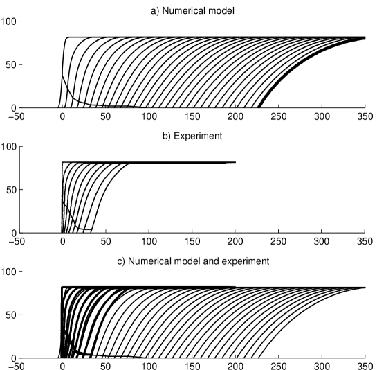
Figure 4: Comparison of experimental and numerical data. Experimental data is based entirely on ([4]). Initial profile given in (23) evolving under (7) with $L=b/v=2.0$. Numerical simulation by standard finite difference scheme, using $N_{s}=750$ spatial subdivisions and $\Delta t=10^{-6}$ timestep, profiles plotted after $N_{t}=12500$ timesteps each. Observe that numerical and experimental profile show very similar evolution. Profile approaches circular steady-state circular geometry with radius $a=131.5$ only much beyond the range of the physical experiment. Location of inflection point is plotted both on experimental and numerical profiles.

5 Conclusions

In this paper we set up the simple PDE model (7) for abrasion under unidirectional (parallel) impacts, based on Bloore’s model [7] for isotropic abrasion. By using the travelling wave ansatz (10) we found circular travelling solutions. After establishing their local (linear) stability analytically, we tested their global attractivity by finite difference simulations and found that they appear to be globally stable. We compared our numerical results to laboratory experiments of Wilson [4] and found good agreement. Our simulation showed that nonconvex profiles may approach their final, circular steady-state geometry via long transients as inflection points may linger above the $x$ axis for extended periods of time. This fact may account for the geological observation of (almost) stationary, non-convex profiles in riverbeds.

6 Acknowledgments

This research was supported by the Hungarian National Science Foundation Grant OTKA K104601.

References

- [1] L. Sklar, W.E. Dietrich WE (2001) Sediment and rock strength controls on river incision into bedrock. Geology 29 (2001) 1087-1090. doi: 10.1130/0091-7613
- [2] L. Sklar, W.E. Dietrich WE (2004) A mechanistic model for river incision into bedrock by saltating bed load Water Resources Research 40 (2004) WO6301. doi: 10.1029/2003WR002496
- [3] A. A. Sipos, G. Domokos, A. Wilson and N. Hovius A Discrete Random Model Describing Bedrock Erosion Mathematical Geosciences 43 (2011) 583-591, DOI: 10.1007/s11004-011-9343-8
- [4] A. Wilson Fluvial bedrock abrasion by bedload: process and form. PhD Dissertation , University of Cambridge, UK (2009).
- [5] A. Wilson, N. Hovius Upstream facing convex surfaces and the importance of bedload in fluvial bedrock incision: observations from Taiwan. Geophysical Research Abstracts 12 EGU2010-4978 (2010)
- [6] G. Domokos, A.A. Sipos and P.L. Várkonyi Continuous and discrete models for abrasion processes Periodica Polytechnica Architecture 40 (2009) 3-8
- [7] F. J. Bloore, The Shape of Pebbles Mathematical Geology 9 (1977) 113-122
- [8] M. Attal, J. Lavé Changes of bedload characteristics along the Marsyandi River (central Nepal): Implications for understanding hillslope sediment supply, sediment load evolution along fluvial networks, anddenudation in active orogenic belts. Spec. Pap. Geol. Soc. Am. 398(2006) 143- 171. doi:10.1130/2006.2398(09).
- [9] A. Wilson, N. Hovius, J. Lavé Solid particle impact abrasion and the formation of bedrock bedforms. Geophysical Research Abstracts 10 , EGU2008-A-03341 (2008)
- [10] K. Hartshorn, N. Hovius,W.B. Dade, R.L. Slingerland RL. Climate-driven bedrock incision in an active mountain belt. Science, 297 (2002) 2036-2038. doi:10.1126/science.1075078