Spurious Shear in Weak Lensing with LSST

Abstract

The complete 10-year survey from the Large Synoptic Survey Telescope (LSST) will image $\sim$ 20,000 square degrees of sky in six filter bands every few nights, bringing the final survey depth to $r\sim 27.5$, with over 4 billion well measured galaxies. To take full advantage of this unprecedented statistical power, the systematic errors associated with weak lensing measurements need to be controlled to a level similar to the statistical errors.

This work is the first attempt to quantitatively estimate the absolute level and statistical properties of the systematic errors on weak lensing shear measurements due to the most important physical effects in the LSST system via high fidelity ray-tracing simulations. We identify and isolate the different sources of algorithm-independent, additive systematic errors on shear measurements for LSST and predict their impact on the final cosmic shear measurements using conventional weak lensing analysis techniques. We find that the main source of the errors comes from an inability to adequately characterise the atmospheric point spread function (PSF) due to its high frequency spatial variation on angular scales smaller than $\sim 10^{\prime}$ in the single short exposures, which propagates into a spurious shear correlation function at the $10^{-4}$–$10^{-3}$ level on these scales. With the large multi-epoch dataset that will be acquired by LSST, the stochastic errors average out, bringing the final spurious shear correlation function to a level very close to the statistical errors. Our results imply that the cosmological constraints from LSST will not be severely limited by these algorithm-independent, additive systematic effects.

1 Introduction

Weak gravitational lensing, or weak lensing for short, is one of the most powerful tools for probing dark matter and dark energy (Albrecht et al., 2006). Distorted by intervening large-scale structures, the otherwise randomly oriented galaxy images encode signatures of dark matter and dark energy in a statistical way, namely through cosmic shear. For a review of weak lensing, see, for example, Bartelmann & Schneider (2001, hereafter BS01). The lensing power spectrum provides a unique tool to distinguish between different cosmological models (Jain & Seljak, 1997; Kaiser, 1998; Hu & Tegmark, 1999).

Since the first detections of the cosmic shear signal by several independent groups (Wittman et al., 2000; Bacon et al., 2000; Kaiser et al., 2000), there has been an explosion of research activity in this field. The most recent analyses have shown that state-of-the-art weak lensing surveys are already probing interesting regions of the dark energy parameter space (Semboloni et al., 2006; Benjamin et al., 2007; Hetterscheidt et al., 2007; Schrabback et al., 2010; Lin et al., 2011; Huff et al., 2011). However, a major limitation of these existing surveys has been their relatively small sky coverage, which results in an insufficient number of galaxies to average out their random shapes and orientations (i.e. to reduce the so-called “shape noise”). Cosmic shear measurements to date are limited by such statistical errors.

As a result, several projects are attempting to overcome this fundamental limitation by significantly increasing the sky coverage. The Dark Energy Survey, the Kilo Degree Survey, Hyper Suprime Cam, LSST(Tyson, 2002) and Euclid projects have all been explicitly designed for weak lensing investigations. The primary improvement of these projects over previous ones is that the cameras they incorporate have very large fields of view, which leads to a much larger survey area and a dramatic improvement in the statistical power of the dataset (Amara & Réfrégier, 2007). When statistical errors become negligibly small in these future surveys, systematics errors become a primary concern.

For weak lensing, there are systematic errors associated with physical effects in the atmosphere and the telescope, and with imperfect algorithms used in the analysis. In this paper, we are mostly interested in quantitatively characterising the former. Systematic errors due to imperfect algorithms are in principle reducible, and will certainly shrink as we gain experience with the near-term upcoming surveys. However, physical effects that are inherent to the system and independent of specific weak lensing algorithms are irreducible and most likely will determine the ultimate limits on cosmological constraints derived from weak lensing.

In the past, the effects of different sources of systematic errors on cosmic shear measurements have usually been calculated by assuming some hypothetical power spectrum for the spurious shear, often in simple functional forms for analytical calculations (Amara & Réfrégier, 2008, hereafter AR08). However, these functional forms may not be well motivated by physics. We make the first attempt to approach the problems in a bottom-up way and simulate the actual measurements to predict the level of systematic errors from first principles. We use LSST as our benchmark survey in this work, but many of the results are general or scalable to other future weak lensing surveys. The LSST Photon Simulator, or PhoSim (Peterson et al., 2009, 2012; Connolly et al., 2010) is used in this work to generate realistic LSST images for this study. In this way, we are able to measure quantitatively the systematic errors generated from various physical effects in a controlled way.

Note that in this paper we only discuss the case of additive shear systematics associated with the projected two-point correlation function on a limited range of angular scales (within the field of a single focal plane). We do not consider weak lensing tomography (Hu, 1999) or higher order statistics (Schneider & Lombardi, 2003; Schneider et al., 2005). The use of these other statistics can impose additional requirements on the level of systematic errors, but on the other hand, if the information is combined properly, it also has the potential of mitigating particular systematic errors that are only present in the projected two-point correlation function.

The paper is organised as follows. A brief review of the canonical framework of weak lensing is given in Section 2. In Section 3 we present a short introduction to LSST and our simulation tool. In Section 4, we lay out a framework for classifying the different physical effects that induce errors in shape measurements. In Section 5, the different sources of errors and their correlation properties are quantified using simulations. Possible sources of spurious shear signals after correcting for the PSF effects are discussed in Section 6, while the results from simulations are presented in Section 7. In Section 8, we discuss the prospect of combining multiple exposures, the implications for the determination of cosmological constraints, and the effect of some of our assumptions on our results. We conclude in Section 9.

2 Weak lensing notation and measurements

In the presence of weak lensing, a galaxy image, having some intrinsic shape, is first sheared by the gravitational potential along the line-of-sight, then convolved with the atmospheric and instrumental PSF before being measured. As an observer, we want to reverse this process: measure the shape of a galaxy from a noisy image, correct for the PSF effects to infer the shear through an estimator, and finally calculate different statistics that are sensitive to cosmology using the shear estimator. For details on the weak lensing formalism, as well as predictions of weak lensing signals from different cosmological models, see BS01.

For this work, following the steps in a data reduction process, we ask the following questions: (1) How do the different physical effects change the measured galaxy shape before any PSF correction has been made? (Section 4, Section 5) (2) To what level can these PSF effects be corrected to infer the correct shear using a conventional algorithm? (Section 6, Section 7) (3) With only the information from two-point shear correlation functions, how do the effects in (1) and (2) scale in the final combined dataset and what does that imply in terms of uncertainties in our predicted cosmological model? (Section 8)

2.1 Weak lensing notation

Throughout the paper we use the following definition for the complex “ellipticity spinor”, $\boldsymbol{\varepsilon}=\varepsilon_{1}+i\varepsilon_{2}$, to parametrise the shapes of objects:

$$\varepsilon_{1}=\frac{I_{11}-I_{22}}{I_{11}+I_{22}}\;,\;\varepsilon_{2}=\frac{2I_{12}}{I_{11}+I_{22}}\;.$$ (1)

where $I_{ij}$ are normalised moments of the object’s light intensity profile $f(x_{1},x_{2})$, weighted by a Gaussian filter $W(x_{1},x_{2})$ to reduce noise:

$$I_{ij}=\frac{\int\int dx_{1}dx_{2}W(x_{1},x_{2})f(x_{1},x_{2})x_{i}x_{j}}{\int\int dx_{1}dx_{2}W(x_{1},x_{2})f(x_{1},x_{2})},\;i,j=1,2\;.$$ (2)

where the width of $W(x_{1},x_{2})$ is chosen to give the maximum signal-to-noise ratio for each individual object.

In this paper, if not otherwise specified, boldface symbols indicate the complex quantities and the magnitude of the complex quantity is specified using the corresponding regular-font symbol (e.g. $\varepsilon=|\boldsymbol{\varepsilon}|=\sqrt{\varepsilon_{1}^{2}+\varepsilon_{2}^{2}}$). A similar notation is used to parametrise shear $\boldsymbol{\gamma}$, where we have $\boldsymbol{\gamma}=\gamma_{1}+i\gamma_{2}$.

We also adopt the standard definitions for calculating the correlation function $\xi_{+,\boldsymbol{XX}}(\theta)$ and power spectrum $C_{\boldsymbol{X}}(\ell)$:

$$\xi_{+,\boldsymbol{XX}}(\theta)=\langle X_{t}(\theta_{0})X_{t}(\theta_{0}+\theta)\rangle+\langle X_{\times}(\theta_{0})X_{\times}(\theta_{0}+\theta)\rangle\;,$$ (3)

$$C_{\boldsymbol{X}}(\ell)=2\pi\int^{\infty}_{0}d\theta\theta\xi_{+,\boldsymbol{XX}}(\theta)J_{0}(\ell\theta)\;,$$ (4)

$$\xi_{+,\boldsymbol{XX}}(\theta)=\frac{1}{2\pi}\int^{\infty}_{0}d\ell\ell C_{\boldsymbol{X}}(\ell)J_{0}(\ell\theta)\;,$$ (5)

where $\boldsymbol{X}$ is a complex spinor (e.g. ellipticity $\boldsymbol{\varepsilon}$ or shear $\boldsymbol{\gamma}$) and the subscripts $t,\times$ indicate an isotropised decomposition of $\boldsymbol{X}$ along the line connecting a particular pair of galaxies. If $\boldsymbol{X}$ is measured in an arbitrary Cartesian coordinate system $\boldsymbol{X}=X_{1}+iX_{2}$ with 1,2 denoting the two axes, then the rotated shear is calculated via $X_{t}=-Re(\boldsymbol{X}e^{-2i\varphi})$ and $X_{\times}=-Im(\boldsymbol{X}e^{-2i\varphi})$, where $\varphi$ is the argument of the vector connecting the pair of galaxies. The angle brackets $\langle\rangle$ indicate an average over all galaxy pairs separated by $\theta$ (with one galaxy located at some $\theta_{0}$). $J_{0}$ is the zeroth-order Bessel function of the first kind. We will use $\xi_{XX}$ as shorthand for $\xi_{+,\boldsymbol{XX}}(\theta)$ for the rest of the paper. For the simulations in this work, we look at angular scales up to the scale of the full LSST focal plane ($\sim 3$ degrees).

2.2 Analysis tools

In all of our analyses of the simulated images, we use the software package Source Extractor (Bertin & Arnouts, 1996) for object detection. We set the following configuration parameters: $\rm DETECT\_MINAREA=5$ and $\rm DETECT\_THRESH=1.5$.

Background estimation, shape measurement, PSF correction and shear estimation were done through the software package IMCAT based on the algorithm derived in Kaiser et al. (1995), Luppino & Kaiser (1997) and Hoekstra et al. (1998), commonly known as KSB. The IMCAT parameters e[0], e[1], gamma[0] and gamma[1] correspond to the ellipticity and shear components $\varepsilon_{1}$, $\varepsilon_{2}$, $\gamma_{1}$ and $\gamma_{2}$ respectively, while the IMCAT parameter $\rm r_{g}$ is used for the width of $W(x_{1},x_{2})$ in Equation 2. Our specific implementation of KSB is similar to the “ES2” method in Massey et al. (2007). We describe briefly the KSB formulae in Appendix B.

3 LSST and PHOSIM

The LSST survey will be the most powerful ground-based weak lensing survey planned for the coming decade. Its revolutionary scale will likely lead the next generation of optical survey designs. We therefore believe that using LSST as the target for this study will enable us to capture the most important issues for future weak lensing surveys.

3.1 LSST design parameters

The optical design of LSST is optimised to cover as much sky as possible while maintaining good image quality (Ivezic et al., 2008). The 8.4-meter aperture and the 9.5-degree² field of view combine to an étendue of $\sim$319.5 m²degree², which is over 10 times larger than that of any previous survey facility. The heart of the instrument is a 64-cm-diameter, 3.2-giga-pixel focal plane. The focal plane is tiled with 189 CCD sensors, each with 4k$\times$4k, 10 $\rm\mu m$ square pixels (each pixel corresponds to an angular scale of 0.2"). The layout of the focal plane geometry is shown in Figure 1.

Good image quality is one of the key components to weak lensing measurements. To ensure that over the entire survey period the instrumental effects that degrade the image quality are kept under control, LSST incorporates an Active Optics System (hereafter AOS), which adjusts the figures and positions of the three reflective optics and the orientation of the camera to correct the wavefront errors.

LSST will take images approximately every 15 – 20 seconds, covering the entire available hemisphere every few days in six optical filter bands. Each of the 2 consecutive 15-second exposures (separated by 4-second readout and shutter open/close) is called a visit. The 2 exposures in a visit will be taken on the same field. From visit to visit, the telescopes will then point to different fields in order to achieve the very wide sky coverage. The 10-year survey will generate an unprecedentedly large amount of data (nearly two thousand 15-second exposures on each field across the 20,000 degree² sky). For cosmic shear measurements, this means reducing the statistical errors from shape noise and cosmic variance by orders of magnitude. As a result, understanding the sources of systematic errors in these data will undoubtedly be a major challenge for LSST.

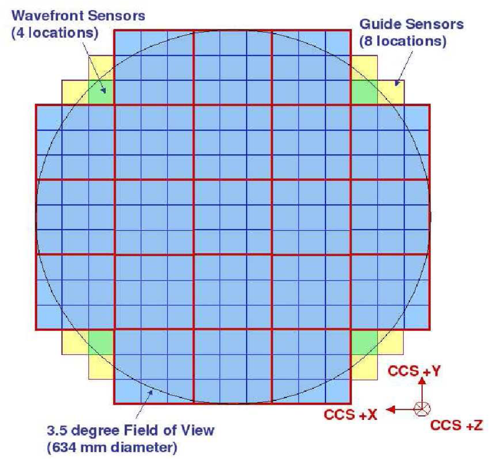
Figure 1: Layout of the LSST focal plane taken from Ivezic et al. (2008). The red and blue thin lines indicate the boundaries for each sensor, where the blue area is the 189 science sensors we use in our focal-plane size simulations. The ellipticity maps from our simulations shown in Figures 3 and 5 correspond to ellipticity values in these areas.

3.2 LSST observation parameters

We extract from catalogues generated by the LSST Operations Simulator (Krabbendam et al., 2010, hereafter OpSim) information about the the observing conditions in an expected LSST weak lensing dataset. OpSim simulates the atmosphere and night sky conditions for individual exposures at the LSST site over 10 years based on weather models, telescope models and optimisation of the survey strategy.

From previous work, it is known that only images with the best image quality contribute to the cosmic shear signal (Hoekstra et al., 2006). As a result, to estimate more accurately the “typical” observing parameters for images that contribute to the final cosmic shear measurement for LSST, we take mediums of the major observation parameters in a subset of the full OpSim catalogue. This subset consists of the 50% of the $r$-band (552–691 nm) data that give the best image quality. From this process we define the “fiducial observing parameters” for a 10-year LSST weak lensing dataset as listed in Table 1. Note that the parameters in Table 1 are specified (when applicable) for $r$ band, while for real weak lensing analyses, $i$-band (691–818 nm) images are likely to be used as well. We carry out all the analyses presented here in $r$ band, but extrapolate the results to $i$ band (see Section 8.1), knowing that the image quality and observing parameters are similar in both bands. In Table 1, the parameter $a_{\rm opt}$ is the designed instrumental PSF size specified in Ivezic et al. (2011) at the elevation that corresponds to the median airmass.

Table 1: Fiducial observing parameters. All parameters are specified for the LSST $r$ band (552-691 nm). These observing parameters are chosen to be typical for obtaining images for weak lensing measurements. The numbers are calculated from the medium values of the best 50% $r$-band exposures. Note that $a_{\rm atm}$ includes the airmass contribution.

Parameter name	Description	Fiducial value
$a_{\rm atm}$	atmospheric seeing	0.56"
$a_{\rm opt}$	instrumental	0.42"
	PSF FWHM
$X_{\rm air}$	airmass	1.2
$B_{\rm sky}$	sky background	640 counts/pixel
$t_{\rm exp}$	exposure time	15 seconds
$b$	Galactic latitude	$-60^{\circ}$
$N$	number of exposures	184

3.3 PHOSIM

To study in detail the expected systematic errors in weak lensing measurements for this survey, existing data from other projects are insufficient in both the data quality and quantity. As a result, simulations become the only way to investigate such problems before the telescope is built. For this study in particular, simulations also enable us to trace the individual sources of systematic errors in a controlled and bottom-up fashion, which is almost impossible to achieve with real data. A few unique features of the simulation process in this work should be emphasised: First, all the physical effects that introduce systematic errors in the shape measurements can be separately turned “on” and “off”. Therefore, we have full control over which actual physical effects are dominant in determining the image shape error. Second, the PSF at the location of a galaxy image can be known exactly by simulating an image with a bright source at that same location. Finally, all physical processes in these numerical experiments are reproducible.

In an earlier attempt to simulate LSST as a complete system using a modified version of existing optics software (Jee & Tyson, 2011), the potential power of studying these issues via simulations has been demonstrated. In this work, we take the analysis one step further and invoke PhoSim as our primary tool for generating simulated images. Unlike the software used in Jee & Tyson (2011), PhoSim is a set of custom-made software designed specifically to represent the LSST’s performance, and simultaneously incorporate many aspects of the project design (e.g. data management software development and scientific studies). PhoSim adopts a photon-by-photon Monte Carlo fast ray-tracing algorithm, which generates images expected for LSST with very high fidelity. In collaboration with the LSST instrumentation teams and multiple science groups, the PhoSim software has been continuously updated and cross-checked to track the most current hardware developments.

PhoSim is part of the end-to-end LSST Image Simulator (ImSim). ImSim simulates the forward process from cosmological models to realistic astronomical images, in which PhoSim is responsible for the last part in this process – the photon propagation from top of the atmosphere down to the CCD sensors and the signal readout. ImSim begins with a catalogue of celestial sources based on large cosmological N-body simulations and detailed Milky Way and Solar System models. A realistic observing environment is then set up by using parameters predicted by the OpSim catalogue. PhoSim then simulates the final “exposure” by tracing individual photons from objects in the catalogue for that part of the sky, through the atmosphere, the telescope, and into the camera to form an image that retains all the major characteristics we anticipate in the LSST data.

We use PhoSim version 3.0 to do all the analyses in this paper. To provide sufficient background material to interpret the results, we describe briefly in Appendix A the major physical models in PhoSim, and refer to Peterson et al. (2012) for further details.

4 Sources of ellipticity errors

Assume the PSF has some finite size $a$ and we measure a PSF-convolved galaxy to have ellipticity $\boldsymbol{\varepsilon}^{m}$, then this $\boldsymbol{\varepsilon}^{m}$ can be broken down to an intrinsic component, a shear component and an additional component from various physical effects associated with counting statistics, the atmosphere and the telescope/camera system. If we assume that all these three components are evaluated for the same measured galaxy size and we are only interested in the small changes in the anisotropy of the galaxy shape, we can write out the following relation in linear additive terms:

$$\boldsymbol{\varepsilon}^{m}=\boldsymbol{\varepsilon}^{i}+\frac{2}{\alpha}\boldsymbol{\gamma}+\boldsymbol{\varepsilon}^{s}\;,$$ (6)

where the first term is the ellipticity of the galaxy convolved with a circular PSF, the second term is the change in $\boldsymbol{\varepsilon}^{m}$ due to shear and the last term is the change in $\boldsymbol{\varepsilon}^{m}$ due to other physical effects. $\alpha$ is a scaling factor to first “de-weight” the ellipticity calculated from the weighted moments (Equation 2) and then account for the effect of the finite-size PSF. The factor of 2 in the second term converts shear into ellipticity (BS01). For infinite resolution (PSF $\sim$ delta function) and ellipticities calculated from unweighted moments ($W=1$), we have $\alpha=1$. For infinite resolution and ellipticities calculated from weighted moments, $\alpha$ is equivalent to two times the shear responsivity $P_{\alpha\beta}^{\gamma}$ defined in Hoekstra et al. (1998).

The correlation function for the measured ellipticity can thus be written out as:

$$\xi_{\varepsilon^{m}\varepsilon^{m}}= \xi_{\varepsilon^{i}\varepsilon^{i}}+\frac{4}{\alpha^{2}}\xi_{\gamma\gamma}+\xi_{\varepsilon^{s}\varepsilon^{s}}$$

$$+2(\frac{2}{\alpha}\xi_{\varepsilon^{i}\gamma}+\frac{2}{\alpha}\xi_{\gamma\varepsilon^{s}}+\xi_{\varepsilon^{i}\varepsilon^{s}})\;.$$ (7)

4.1 Non-stochastic and stochastic errors in ellipticity measurements

Here we present a concept for classifying $\boldsymbol{\varepsilon}^{s}$ similar to that in Jain et al. (2006). This classification scheme is especially important for analyses of multi-epoch datasets such as LSST – this is the first step towards understanding the nature of different sources of systematic errors in shear measurements. Two major classes of physical effects combine to give $\boldsymbol{\varepsilon}^{s}$. We use the terms “non-stochastic” and “stochastic” to refer to these two classes of errors.

Non-stochastic errors are those that are either fixed in space and time, or vary with characteristic patterns over multiple exposures. Stochastic effects, on the other hand, induce errors that change randomly from exposure to exposure with no correlation in time. For non-stochastic errors, because they show repeated patterns from frame to frame, one does not benefit from averaging over multiple independent exposures; however, this repeating feature also means that they potentially can be characterised very well when one properly combines the multi-epoch dataset. Stochastic errors are exactly the opposite: randomness implies one can only model them with data from limited information in a single exposure, but via some form of averaging of the multiple exposures on the same field, the errors are likely to cancel each other.

Table 2: Classification of the major physical effects that introduce errors in shape measurements. The difference between non-stochastic and stochastic optics errors is described in Section 4.

Non-stochastic effects	Stochastic effects
Optics design	Counting statistics
Non-stochastic optics errors	Stochastic optics errors
	Tracking errors
	Atmospheric effects

In Table 2, we identify the major non-stochastic and stochastic effects that are modeled in PhoSim and are most likely to contribute to $\varepsilon^{s}$. We also provide in Appendix A brief descriptions of how each of these effects is modelled in PhoSim. There are some physical effects that may be present and are not yet modeled in the current PhoSim, but we believe they will not contribute significant. The effects listed in Table 2 should comprise the great majority of the sources of error for weak lensing measurements with LSST.

In most existing weak lensing data, non-stochastic effects dominate the error; therefore the origins of these systematic errors are historically better understood. For example, Jarvis et al. (2008) were able to model the PSF patterns of telescope aberrations with low order functional forms. Stochastic effects, being relatively small in existing data, have not been studied in detail. Only a few pioneering studies have tried to understand the stochastic effects under simple cases: Paulin-Henriksson et al. (2008) and Zhang (2010) studied the noise contribution to shape measurement due to counting statistics and pixelation, while De Vries et al. (2007) investigated the atmosphere-induced ellipticity and its time dependence.

Note that this classification scheme is only valid under a well-defined survey since it depends on the cadence of the survey and other operational issues. In this paper we are assuming the as designed LSST survey mode (Section 3.1), where the minimum time between consecutive visits on the same patch of sky is approximately 30 minutes (Ivezic et al., 2011). This means that the telescope has experienced at least $\sim$50 different pointings between the two consecutive visits and is looking through a very different column of atmosphere each time. Under this scenario, most of the physical effects we discussed are truly stochastic, or at least stochastic to a very high level between visits. For the two exposures in the same visit, due to the close separation in time, stochasticity is not guaranteed for all effects – we discuss in Appendix D how this factor may be estimated for the spurious shear correlation function in the combined dataset.

4.2 Practical considerations

Real galaxies have intrinsic shapes, and will be subject to cosmic shear, so that in Equation 6, $\boldsymbol{\varepsilon}^{i}$ and $\boldsymbol{\gamma}$ are not generally equal to zero. To average over these effects at the statistical level sampled by LSST, we would need to simulate $\sim$200 images of roughly four billion galaxies in each test. This is computationally impractical, so we adopted a simpler approach described below.

Note from Equations 6 and 7 that if we set up simulations so that $\boldsymbol{\varepsilon}^{i}=\boldsymbol{\gamma}=0$, we can avoid the contribution from $\boldsymbol{\varepsilon}^{i}$ and $\boldsymbol{\gamma}$ in the observable $\boldsymbol{\varepsilon}^{m}$, and directly measure $\boldsymbol{\varepsilon}^{s}$ and $\xi_{\varepsilon^{s}\varepsilon^{s}}$ unambiguously. This suggests that our problem is equivalent to asking the following question:

Under zero shear, what is the anisotropic component of the spurious ellipticity $\boldsymbol{\varepsilon}^{s}$ induced by a certain physical effect on a circular object of $\boldsymbol{\varepsilon}^{i}=0$ and what are the correlation properties $\xi_{\varepsilon^{s}\varepsilon^{s}}$ of those spurious ellipticities?

That is, we do not measure the ellipticity on a fully realistic galaxy population with a distribution of shapes, sizes and brightnesses; instead, simple circular “galaxies” are used as “test particles” for the entire population of galaxies. We show below that this approach is justified for our purposes.

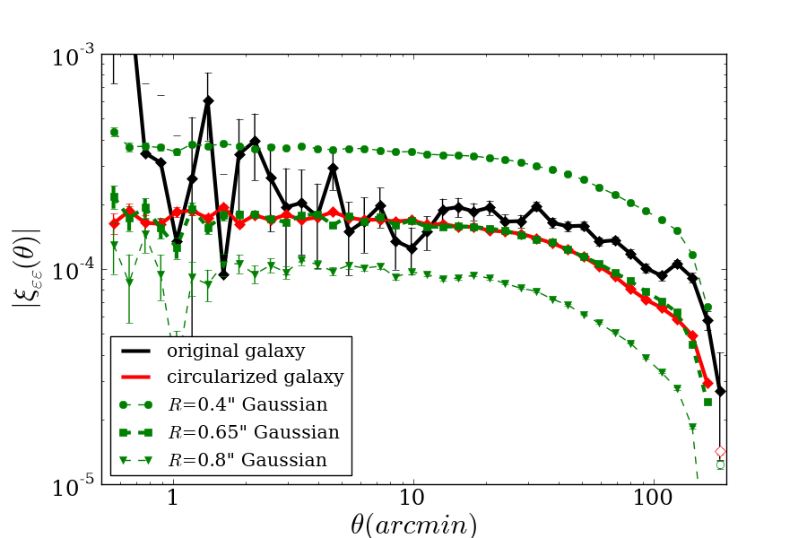
Figure 2: Ellipticity correlation function for different samples of simulated galaxies. Black shows the ellipticity correlation function for a realistic galaxy sample, while red shows the same function measured from the circularised counterpart of the realistic galaxy sample. Green curves are measured from samples of circular Gaussian shapes of different sizes. The green curve measured from circular Gaussians of 23rd $r$-band magnitude and $R$=0.65" (green square) agree approximately in level and shape with the black and red curves, where $R$ is the FWHM size of the Gaussian profile. This demonstrates (1) shape noise is uncorrelated and (2) we can use the circular Gaussian shape with $r$-band magnitude 23 and $R$ =0.65" as the “fiducial galaxy” to measure the spatial correlations of the response of the entire galaxy population.

In Figure 2, we simulate a representative galaxy sample from the PhoSim sky catalogue and measure the ellipticity correlation function $\xi_{\varepsilon^{m}\varepsilon^{m}}$ from a typical single exposure. We then “circularise” these galaxy images at the input catalogue level before entering the atmosphere so that they retain all the characteristics, such as size, brightness, redshift and spectral energy distribution (SED) in the original sample, but lose the shape information. Although the original sample shows a noisier ellipticity correlation function, the circularised sample roughly agrees with it in both level and shape. The agreement between the ellipticity correlation functions measured from the original galaxies and the circularised galaxies demonstrates that shape noise is not spatially correlated; thus it should play no role in the correlation function as expected. In other words, we have $\xi_{\varepsilon^{i}\varepsilon^{i}}=\xi_{\gamma\gamma}=\xi_{\varepsilon^{i}\gamma}=\xi_{\varepsilon^{s}\gamma}=0$ for both samples. The slightly lower red curve is mainly due to the small $\xi_{\varepsilon^{i}\varepsilon^{s}}$ term that is present only in the original galaxy sample. We show that we can isolate $\xi_{\varepsilon^{s}\varepsilon^{s}}$ in the $\xi_{\varepsilon^{m}\varepsilon^{m}}$ using the circularised galaxy sample.

Table 3: Fiducial galaxy characteristics specified in $r$ band. The representative sample of weak lensing galaxies can be collapsed into the fiducial galaxy and reproduce the same ellipticity correlation function – on average, the fiducial galaxy reacts to the PSF effects the same way as the population of galaxies.

Parameter name	Description	Fiducial value
$m$	AB magnitude	23
$S$	total signal counts	$\sim$ 2600 counts
$R$	Gaussian FWHM	0.65"
$n_{\rm gal}$	number density	$\sim$ 5.5 $/{\rm arcmin^{2}}$
SNR	signal-to-noise ratio	8.33

To further simplify the problem, the distribution of circular galaxies is collapsed into a single circular Gaussian shape. By exploring the size-magnitude parameter space, we find that using roughly the average magnitude, size and number density of the original sample, we can recover the ellipticity correlation of the circularised galaxy sample. For the rest of this paper, we will refer to this special circular Gaussian as the “fiducial galaxy.” Figure 2 shows the ellipticity correlation functions for three different sizes of circular Gaussian shapes, with the middle one (square) being the fiducial galaxy. The characteristics of the fiducial galaxy are listed in Table 3.

The construction of the fiducial galaxy is an approximation, but is appropriate for our analyses with the following caveats. First, by taking the ellipticity results from a circular galaxy ($\boldsymbol{\varepsilon}^{i}=\boldsymbol{\gamma}=0$) as a general result for the whole galaxy population, we are assuming that the average ellipticity error on the population of galaxies is approximately the ellipticity error on the average galaxy in the population. This is ignoring the fact that certain algorithms may tend to measure the ellipticity of a galaxy more accurately when the galaxy is more circular or more elliptical. This intrinsic-ellipticity-dependent error may introduce additional errors in the ellipticity measurements. We ignore them because these errors are algorithm-dependent, and are spatially uncorrelated, i.e. they only contribute a small addition contribution to shape noise. Second, by choosing a Gaussian profile for the fiducial galaxy rather than a more realistic Sersic-type profile, we are assuming our ellipticity measurement method performs equally well on Gaussian profiles and realistic galaxy profiles. This again is to eliminate the algorithm-dependence coupling to the problem and also important later for shear measurements as discussed in Section 6.

5 Quantifying errors on ellipticity measurements

In this section, if not otherwise specified, the measured ellipticity on any simulated galaxy image is effectively an “ellipticity error” generated from a certain physical effect, for reasons we have explained in Section 4.2 ($\boldsymbol{\varepsilon}^{i}=\boldsymbol{\gamma}=0$). Thus we omit the superscripts in our notation and use $\boldsymbol{\varepsilon}$ ($\xi_{\varepsilon\varepsilon}$) instead of $\varepsilon^{s}$ ($\xi_{\varepsilon^{s}\varepsilon^{s}}$) or $\varepsilon^{m}$ ($\xi_{\varepsilon^{m}\varepsilon^{m}}$).

Also, for all ellipticity measurements, we define the quantity $\sigma[\boldsymbol{\varepsilon}]$ to be a measure of the uncertainty in ellipticity measurements due to a certain physical effect. $\sigma[\boldsymbol{\varepsilon}]$ is defined as the square-root of the quadrature sum of the standard deviation of individual $\varepsilon_{1}$ and $\varepsilon_{2}$ distributions (as opposed to the standard deviation of $\varepsilon$):

$$\sigma[\boldsymbol{\varepsilon}]=\sqrt{\sigma_{\varepsilon_{1}}^{2}+\sigma_{\varepsilon_{2}}^{2}}\;.$$ (8)

5.1 Non-stochastic effects

5.1.1 Simulations

To examine the non-stochastic effects, we generated two sets of simulations. Each set of simulations consists of one or more full LSST focal planes. In all of the simulations, since we need to “turn off” the atmospheric effects, we convolve the fiducial galaxies with a circular Gaussian before running the simulations to ensure that the observed galaxies have the same size as a fiducial galaxy observed under the fiducial observing conditions. To suppress the contribution from counting statistics errors in the measurements, all objects are generated with high SNR at $\sim 160$.

In the first set of simulations, we simulate the “as designed instrument” by including only the optics design, isotropic charge diffusion in the CCD detectors, and pixelisation. In the second set of simulations, we include non-stochastic perturbations to the optics due to solid body misalignments, surface perturbations of the major optics elements, and warping and misalignment of the individual sensors in the focal plane (see Table 5 for approximate levels of the major perturbations). Twenty focal-plane size images with different Gaussian random realisations of these errors are generated in order to capture the effects in a “typical” LSST observations.

5.1.2 Results

In Figure 3 (a), we show the ellipticity magnitude $\varepsilon$ measured from the simulations across the LSST focal plane for the as designed instrument. When non-stochastic optics error is induced, the measured ellipticity changes. One example in the set of simulation is shown in Figure 3 (b), where the change in ellipticity due to a certain set of optics errors is shown.

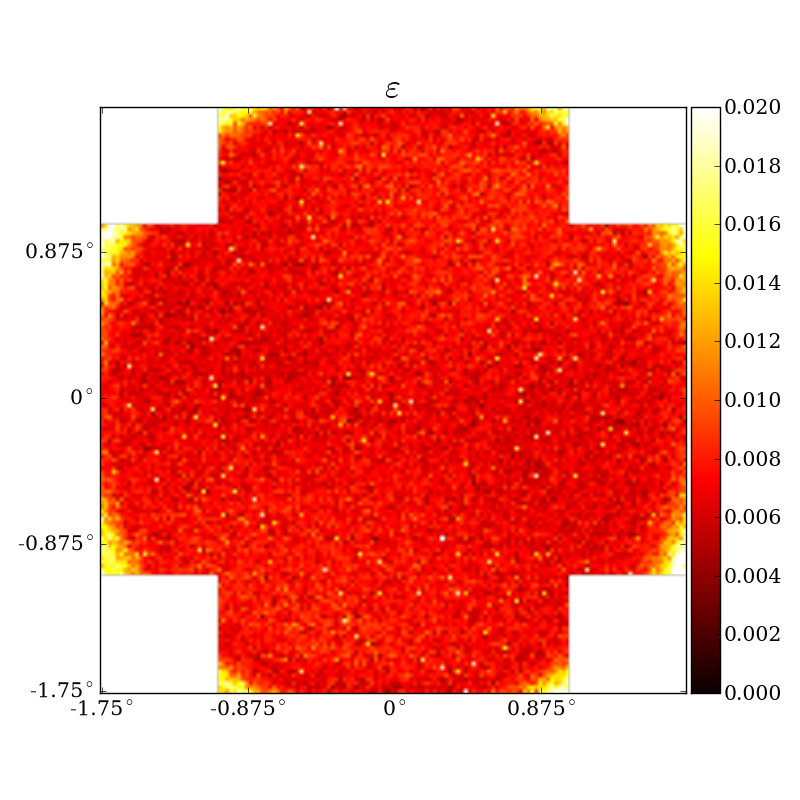
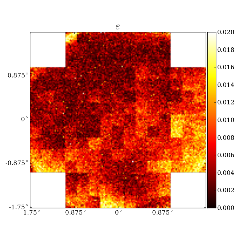
Figure 3: Ellipticity magnitude $\varepsilon$ measured from the fiducial galaxies over the LSST focal plane for the (a) optics design and (b) one example of adding non-stochastic optics errors. All non-stochastic optics effects induce ellipticity magnitudes $<$0.02 for most of the field. Greater ellipticites are mainly near the edges. The large-scale variations come from perturbations of the positions and surface heights of the mirrors and lenses, while the variation in the focal plane height contributes to the visible boundaries between individual CCDs.

The distribution of $\varepsilon$ for the two sets are plotted in Figure 4 (a) with arbitrary normalisations. The corresponding $\sigma[\boldsymbol{\varepsilon}]$ values of these distributions after correcting for the counting statistics are listed on the plot. We measure $\sigma[\boldsymbol{\varepsilon}]\sim 7\times 10^{-3}$ for the design, $\sigma[\boldsymbol{\varepsilon}]\sim 6\times 10^{-3}$ for the non-stochastic optics effects. The total ellipticity contribution from all non-stochastic effects on the fiducial galaxy is $\sigma[\boldsymbol{\varepsilon}]\sim 9\times 10^{-3}$.

The median absolute ellipticity correlation function $|\xi_{\varepsilon\varepsilon}|$ measured from the fiducial galaxies in all the simulations is plotted in Figure 4 (b) for the design and for the non-stochastic optics effects added. The total ellipticity correlation function for all effects in this “non-stochastic” class is also shown. The correlation function for the design is at the level $\sim 1.5\times 10^{-5}$ with a rather flat shape. Adding non-stochastic effects almost doubles the level of the correlation function.

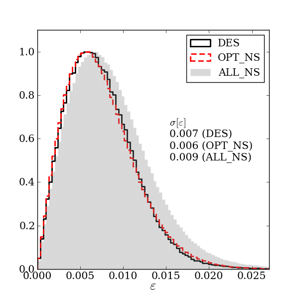
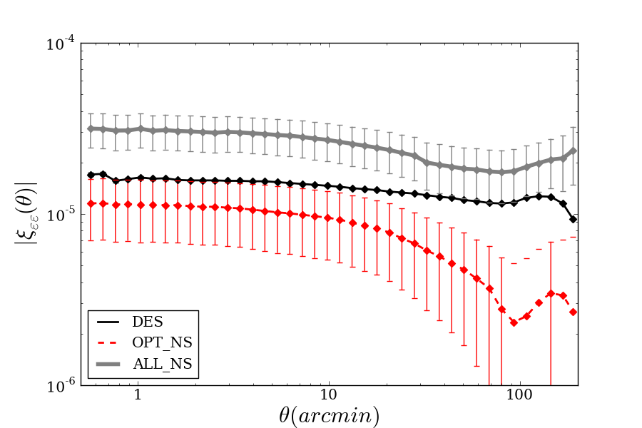
Figure 4: The following abbreviations are used for the different sources of ellipticity errors: DES (design), OPT_NS (non-stochastic optics effects) and ALL_NS (all non-stochastic effects). (a) Distribution of the ellipticity magnitude measured for the fiducial galaxies when different non-stochastic effects are added. (b) Absolute correlation function of the ellipticity errors for the fiducial galaxies when different non-stochastic effects are added. The red curve is the median value for 20 different realisations of the non-stochastic optics effects.

Note that Figure 4 may not be characteristic of other telescopes, since we have utilised a large amount of LSST-specific information about the optics configuration and engineering tolerances (Ivezic et al., 2011). However, the main message from this section is the demonstration that for future large telescopes with designs similar to LSST, the non-stochastic spurious ellipticity correlation will be at a low level compared with existing telescopes (see Jarvis & Jain, 2004, for example).

5.2 Stochastic effects

5.2.1 Simulations

To examine the contributions of stochastic effects, we use one realisation of the non-stochastic optics errors in the previous simulations and then add on stochastic contributions that vary randomly from exposure to exposure. Non-stochastic contributions to the ellipticities are later subtracted component-wise from the measured ellipticities to obtain the stochastic contribution.

For each of the four stochastic effects listed in Table 2, we generate a set of 20 focal-plane-size simulations with fiducial galaxies distributed over the field. The input parameters to the 20 simulations in each set are controlled so that each of the other three effects are “turned off” and only one effect is “turned on” – only parameters associated with that one effect are allowed to vary. In addition, we generate one set of simulations (20 focal-plane-size image), where the four stochastic effects are all turned on. These images are used in Section 7 for shear measurement tests. We describe below the prescriptions for how we set the parameters for each of the effects in the simulations.

Counting statistics

is the largest stochastic source of noise in these single exposures. It is also the only effect that is stochastic in both space and time, which prohibits it from being corrected through PSF modelling.

The relevant measure for counting statistics is the SNR of an object, which we can calculate straightforwardly for a circular Gaussian profile given the total signal counts $S$, object FWHM size $R$, background counts $B_{\rm sky}$ and apparent object FWHM size $R^{m}$:

$${\rm SNR}=\frac{0.7\times S}{\sqrt{0.7\times S+\pi(1.34\times R^{m})^{2}\times B_{\rm sky}}}$$ (9)

Here we use a typical aperture radius of $\sim$1.34 times the FWHM of the apparent object size $R^{m}$, containing $\sim$70% of the source counts. For circular Gaussian, the apparent object size $R^{m}$ can be approximated as the object size $R$ convolved with a circular Gaussian with FWHM size equal to the PSF size $a$:

$$(R^{m})^{2}=R^{2}+a^{2}$$ (10)

where $a$ can be estimated by adding to $a_{\rm atm}$ in quadrature the instrumental PSF contribution $a_{\rm opt}$:

$$a=\sqrt{a_{\rm atm}^{2}+a_{\rm opt}^{2}}$$ (11)

In this section, we fix $S$, $R$, $B^{\rm sky}$ and $a$ to the fiducial values in Tables 1 and 3. In Section 5.3, we explore the full SNR parameter space. The 20 focal-plane-size images in this set are identical except that different photons are drawn from the galaxy and therefore travel slightly different light-paths.

Stochastic optics effects

are the residual optics errors after AOS correction that do not show repeatable patterns from exposure to exposure. The 20 focal-plane-size images in this set are identical except that the optics perturbations are varied from frame to frame within the level allowed by the adopted tolerances listed in Table 5.

Tracking errors

occur due to imperfect tracking of the telescope during the exposure. They cause the measured object shape to be slightly elongated in the direction of the sky rotation. The 20 focal-plane-size images are identical except that a different tracking error trajectory within the adopted tolerances described in Section A.2 is assigned to each realisation.

Atmospheric effects

are slightly more complicated to model. For the same assumed fiducial seeing in all 20 simulations, different realisations of the atmosphere are generated by different combinations of the structure function, outer scale, wind speed and wind directions over the multiple atmospheric layers. The 20 focal-plane-size images are identical except that a different combination of these parameters is used.

For the first three sets of simulations, since the atmosphere is turned off, all objects are convolved with a circular Gaussian before we run the simulator so that the measured object size is the same as if it had propagated through the atmosphere. Similar to Section 5.1.1, for all sets except the first, objects are generated with high SNR at $\sim 160$ to suppress contribution from counting statistics errors in the measurements. The ellipticity of each object is measured and the mean ellipticity for each object over the 20 realisations is taken as the non-stochastic contributions and subtracted component-wise to yield the stochastic ellipticity component.

5.2.2 Results

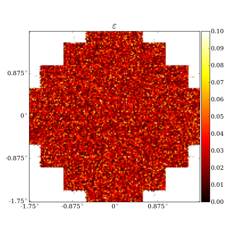
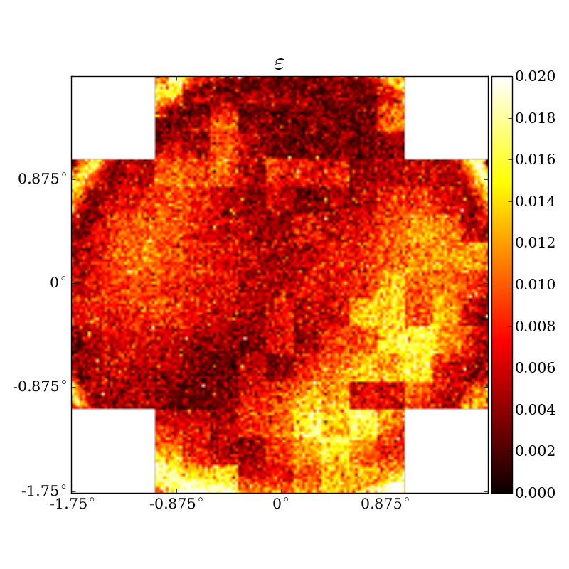
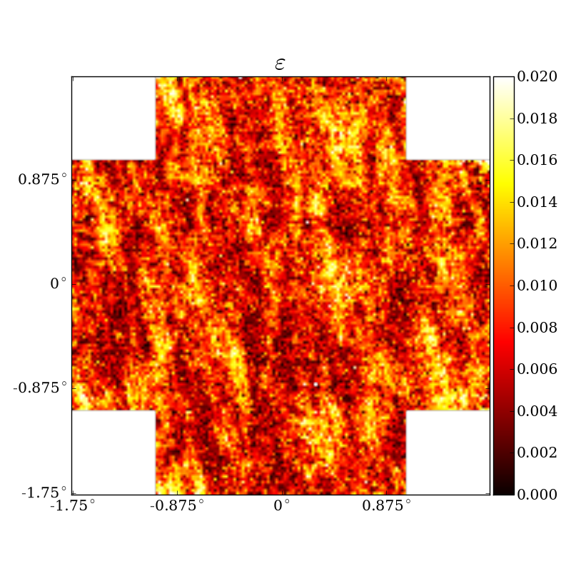
Figure 5: Ellipticity magnitude $\varepsilon$ measured from the fiducial galaxies over the LSST focal plane for four stochastic effects: (a) counting statistics, (b) tracking errors, (c) stochastic optics errors and (d) atmospheric distortions. In each case, the colour bars are adjusted to best show the ellipticity spatial pattern. Since these effects are stochastic, we show only one representative realisation of the random process to illustrate the kind of ellipticity pattern induced by each effect. Among the four, (a) counting statistics induces the highest level of errors and show “missing” sensors on the edge of the field due to the fact that vignetting causes the fiducial galaxies to be undetectable at those positions.

Figure 5 shows one example of the absolute ellipticity errors in each of the four sets. The colour mapping for the four plots are adjusted to best illustrate the spatial patterns and absolute ellipticity levels. Note that in Figure 5 (a) the CCDs in the corner of the field are missing. This is because the fiducial galaxies have very low SNR at those vignetted locations. In a more realistic field, brighter galaxies will still be detected there.

Distributions of the magnitudes of the stochastic ellipticity errors $\varepsilon$ measured from the four sets of simulations are plotted in Figure 6 (a). Each of the curve is normalized so that it peaks at . Also overlaid is the total stochastic ellipticity error distribution. The corresponding $\sigma[\boldsymbol{\varepsilon}]$ values of these distributions after correcting for counting statistics¹¹ are listed on the plot. Figure 6 (c) is a zoomed-in view of Figure 6 (a) on the lower ellipticity values. Clearly, in a single exposure the dominant error contribution to the shape measurements for a fiducial galaxy is counting statistics, giving $\sigma[\boldsymbol{\varepsilon}]\sim 1.1\times 10^{-1}$. The atmospheric effects and the stochastic optics effects are at similar levels and are the second and third largest contributors, giving $\sigma[\boldsymbol{\varepsilon}]\sim 1.2\times 10^{-2}$ and $\sigma[\boldsymbol{\varepsilon}]\sim 1.1\times 10^{-2}$ respectively. Tracking errors are the most insignificant effect of the four, with $\sigma[\boldsymbol{\varepsilon}]\sim 5\times 10^{-3}$. The total stochastic ellipticity uncertainty when all effects are turned on is $\sigma[\boldsymbol{\varepsilon}]\sim 1.3\times 10^{-1}$. Note that the total non-stochastic ellipticity error discussed in Section 5.1 is more than an order of magnitude smaller than the total stochastic ellipticity errors.

We now turn to the median correlation functions of these four stochastic ellipticity error components, shown in Figure 6 (b), along with the total stochastic ellipticity error correlation function. The error bars in each case show the standard deviation of the 20 realisations divided by $\sqrt{20}$. The first observation is that although counting statistics errors dominate in the ellipticity error as shown in Figures 5 and 6 (a), they are completely uncorrelated. They oscillate rapidly but are always consistent with zero. This is of course expected – regardless of the SNR of the measured objects, counting statistics makes no contribution to the correlation function. Tracking errors, on the contrary, being the lowest in Figure 6 (a), contribute to a small but non-zero correlation at the $10^{-5}$ level. The stochastic optics effects generate ellipticity correlations slightly below the $10^{-4}$ level while the atmospheric effects contribute to a similar level of ellipticity correlation with a steeper shape as can be seen more clearly in Figure 6 (d), the zoomed-in view for Figure 6 (b). The total ellipticity correlation function is thus dominated by the atmosphere component at small scales and then a combination of the stochastic optics errors and the atmospheric effects at larger scales. Also notice that the non-stochastic component is approximately an order of magnitude smaller than the total stochastic ellipticity correlation in a single exposure.

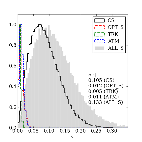
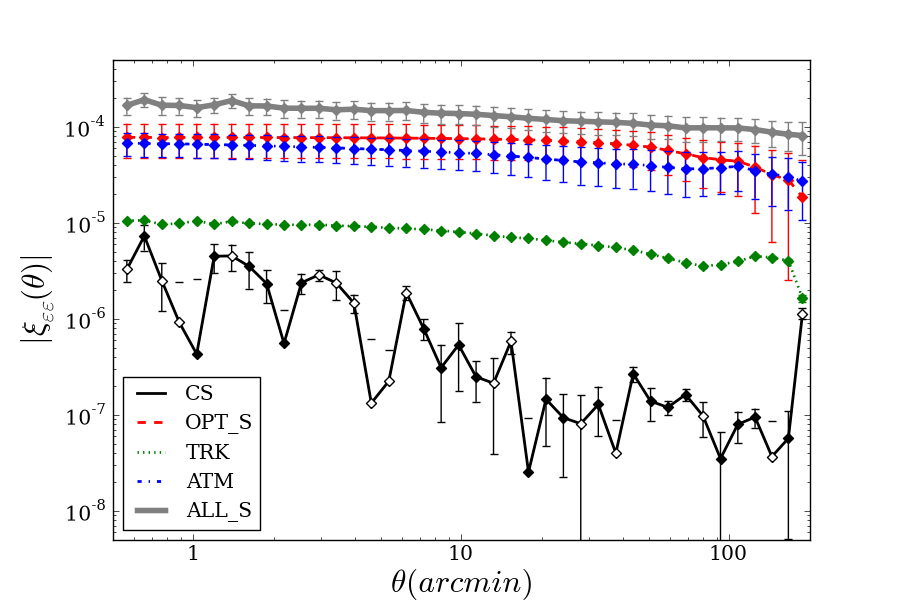
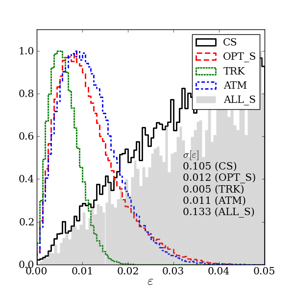
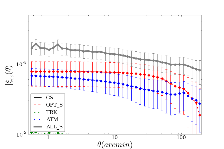
Figure 6: The following abbreviations are used for the different sources of ellipticity errors: CS (counting statistics), OPT_S (stochastic optics effects), TRK (tracking errors), ATM (atmospheric effects), and ALL_S (all stochastic effects). (a) Distribution of the ellipticity magnitude measured for the fiducial galaxies when different stochastic effects are added. The grey shaded area indicates the ellipticity magnitude distribution from all the stochastic effects together. (b) Absolute correlation function of the ellipticity errors for the fiducial galaxies when different stochastic effects are added. Note that all curves plotted for the stochastic effects are the median value for 20 different realisations, with the error bars showing the standard deviation of the 20 realisations divided by $\sqrt{20}$. Negative values are plotted with open symbols. (c) is a zoomed-in view of (a) on the lower ellipticity values and (d) is a zoomed-in view of (b) on the higher correlation function curves.

5.3 Discussion

Up to this point, we have quantified $\sigma[\boldsymbol{\varepsilon}]$, the expected levels of errors in ellipticity measurements due to different physical effects for a typical LSST single exposure. These results can be scaled to other observing conditions and source distributions as a first-order estimation for the uncertainties in ellipticity measurements in another dataset. The two major quantities that govern the scaling of $\sigma[\boldsymbol{\varepsilon}]$ and $\xi_{\varepsilon\varepsilon}$ for a certain dataset are the average observed object size $R^{m}$ (Equation 10) and the average SNR (Equation 9) of the objects. The level of counting statistics contribution to ellipticity errors $\sigma[\boldsymbol{\varepsilon}]$ is expected to scale with some function of SNR, while ellipticity errors from all the other effects scale with $(R^{m})^{-2}$. For $\xi_{\varepsilon\varepsilon}$, on the other hand, the counting statistics contribution is essentially zero, while all other components scale with $(R^{m})^{-4}$.

Note also that in general the measured level of the correlation function is lower than what is expected for a naive assumption of $|\xi_{\varepsilon\varepsilon}|\sim\sigma[\boldsymbol{\varepsilon}]^{2}$. This is because the distortions of the galaxies are usually only partially correlated in space. The degree of correlation, which is governed by the physical mechanism that induces the correlation, determines how close $|\xi_{\varepsilon\varepsilon}|$ approaches $\sigma[\boldsymbol{\varepsilon}]^{2}$.

To determine the scaling of $\sigma[\boldsymbol{\varepsilon}]$ with SNR, we perform a series of simulations similar to the first set of simulations (i.e. counting statistics) in Section 5.2.1, but vary the input galaxy’s size and magnitudes over the range $R=$ [0" (point source), 0.5", 0.7", 0.85", 1.0", 1.5", 2.0"] and $m=$ [18, 19, 20, 21, 22, 23, 24] to cover a nominal galaxy population and plot $\sigma[\boldsymbol{\varepsilon}]$ as a function of the object’s SNR. The results are illustrated in Figure 7. We find that even for the wide range of size and brightness sampled, the ellipticity errors for all objects lie on a power law curve of index $\sim-1$, described by the fit:

$$\sigma[\boldsymbol{\varepsilon}_{CS}]\approx 0.875\times{\rm SNR}^{-0.9995}\approx\frac{0.875}{\rm SNR}\;,$$ (12)

where the subscript $CS$ indicates the ellipticity uncertainty due to counting statistics errors only. Equation 12 is consistent with the analytical predictions and numerical simulations (Paulin-Henriksson et al., 2008; Réfrégier et al., 2012) in previous studies.

In Figure 7, we show the breakdown of $\sigma[\boldsymbol{\varepsilon}]$ into different components for a galaxy of FWHM size $\sim 0.65$" under fiducial LSST observing conditions (Table 1) as a function of the SNRs of the objects. The top axis $m^{*}$ shows the corresponding $r$-band AB magnitude for objects at that SNR. The errors due to all non-stochastic effects and the errors due to all stochastic effects except counting statistics are by definition independent of the SNR of the galaxy, therefore they are represented by horizontal lines on the plot. The total errors from stochastic effects are derived by adding the level of counting statistics contributions and other stochastic errors in quadrature.

Under the assumption that these individual noise terms are approximately independent from one another, we can now estimate the uncertainty in ellipticity measurements of an arbitrary galaxy under an arbitrary scenario by scaling the results from our tests with the fiducial galaxies and conditions, which we denote by the subscript “0” in the following steps:

1. Calculate the galaxy’s SNR, which depends on $R^{m}$, $S$, $a$ and $B_{\rm sky}$, and scale the counting statistics errors on the ellipticity from the fiducial case via:

   $$\sigma[\boldsymbol{\varepsilon}]\propto\frac{SNR_{0}}{SNR}\;.$$ (13)

2. Calculate the contributions from all other effects by scaling the results in Sections 5.1 and 5.2 by the measured galaxy size:

   $$\sigma[\boldsymbol{\varepsilon}]\propto\left(\frac{R^{m}_{0}}{R^{m}}\right)^{2}\;.$$ (14)

3. All stochastic components are further scaled by the exposure time:

   $$\sigma[\boldsymbol{\varepsilon}]\propto\sqrt{\frac{t_{exp,0}}{t_{exp}}}\;.$$ (15)

4. Add the individual components in quadrature to yield an estimate of the total ellipticity uncertainty in the measurement. Note, however, that the simple assumption that all effects are decoupled breaks down at the low SNR end, where the errors are no longer small and cannot be linearly decomposed into the different components.

It is straightforward to also estimate the ellipticity error correlation function of a population of galaxies:

1. Since counting statistics errors do not correlate, we do not need to account for a correlation function for them.

2. Scale the individual correlation functions in Figures 4 and 6 by the average $R^{m}$ of objects in the frame:

   $$\xi_{\varepsilon\varepsilon}\propto\left(\frac{R^{m}_{0}}{R^{m}}\right)^{4}\;.$$ (16)

3. Scale the stochastic components of the individual correlation functions by $t_{exp}$:

   $$\xi_{\varepsilon\varepsilon}\propto\frac{t_{exp,0}}{t_{exp}}\;.$$ (17)

4. Add the individual components to yield the total ellipticity correlation function.

These scaling relations serve as first-order estimates of the ellipticity errors and error correlations.

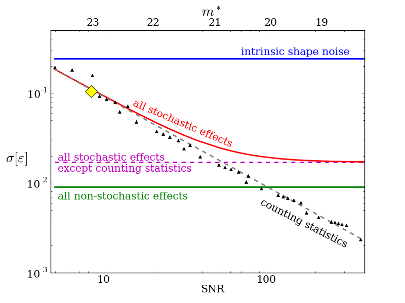
Figure 7: Uncertainties of ellipticity measurements induced by counting statistics errors for objects in a large range of size and magnitudes is labeled by the black triangles, which is well fit by a function of the objects’ SNR as shown with the grey dashed line. If all the parameters other than magnitude ($m$, or effectively, $S$) are held fixed, then the bottom SNR axis corresponds to the $r$- band AB magnitudes labeled on the top axis $m^{*}$. The yellow diamond at $m^{*}=23$ is where the fiducial galaxy is located. Under the same assumption that we only vary the object’s magnitude along the x-axis, we can then plot the ellipticity uncertainties induced by all the other physical effects discussed in this paper as horizontal lines since these errors depends only on the object’s size. Finally, the level of intrinsic shape noise is indicated by the solid blue line.

6 Sources of spurious shear

After measuring the ellipticities of the galaxies ($\boldsymbol{\varepsilon}^{m}$ in Equation 6), the next step, following Equation 18, is to estimate the PSF-induced ellipticity errors $\boldsymbol{\varepsilon}^{s}$, estimate the scaling factor $\alpha$ and calculate the shear estimator $\boldsymbol{\hat{\gamma}}$:

$$\boldsymbol{\hat{\gamma}}=\frac{\alpha}{2}(\boldsymbol{\varepsilon}^{m}-\boldsymbol{\varepsilon}^{s})=\boldsymbol{\gamma}+\frac{\alpha}{2}\boldsymbol{\varepsilon}^{i}.$$ (18)

The first part of Equation 18 represents operationally how one would calculate $\boldsymbol{\hat{\gamma}}$ and the second part comes from rearranging Equation 6. When averaging $\boldsymbol{\hat{\gamma}}$ over a large number of galaxies, we recover the true shear, or $\langle\boldsymbol{\hat{\gamma}}\rangle=\boldsymbol{\gamma}$. As described in Section 4.2, since we have set both shear and intrinsic ellipticity to zero in our simulations, any non-zero shear measurement from Equation 18, even without averaging over an ensemble of galaxies, indicates mis-estimation of $\boldsymbol{\varepsilon}^{s}$ and/or $\alpha$. In other words, any measured shear from our simulations is spurious. In the remainder of this section, we use $\boldsymbol{\gamma}^{s}$ and $\xi_{\gamma^{s}\gamma^{s}}$ to indicate the spurious shear and their correlation functions. As opposed to previous ellipticity measurements, we only show results for $\xi_{\gamma^{s}\gamma^{s}}$ (rather than single $\boldsymbol{\gamma}^{s}$ measurements), and propagate them directly into uncertainties of the inferred cosmological model in Section 8.2.

Operationally, three separate steps are involved in calculating the terms of Equation 18 that are prone to systematic effects: PSF modelling (estimating $\boldsymbol{\varepsilon}^{s}$), “deconvolving” with the PSF (properly removing the effect of the PSF in estimating intrinsic galaxy shape) and converting the measurement to shear (estimating $\alpha$). The first step is related to properly modelling the physical effects discussed previously, while the latter two steps are determined by choices of algorithms. We use the terms “spurious shear from PSF modelling” and “spurious shear from shear measurement algorithms” to refer to these two classes of errors.

Given a perfectly known PSF, an imperfect algorithm can still render spurious shear. Several works have studied the effectiveness of different PSF deconvolution algorithms and quantified the errors in shear measurements (Heymans et al., 2006; Massey et al., 2007; Bridle et al., 2010; Kitching et al., 2012a, b). This spurious shear studied in previous work (“spurious shear from shear measurement algorithms” in our classification) is not necessarily intrinsic to the measurement, and is therefore not the main interest of this paper. We choose to use KSB, one of the most popular weak lensing algorithms, as our test method, but design the simulations and analyses as described below to eliminate some of the known flaws in this method. All of our results can thus be viewed as the best possible results achievable by a KSB pipeline. In principle, more sophisticated pipelines should do even better.

As mentioned in Section 4.2, we choose to use simple circular Gaussians as galaxies to perform our analyses. In terms of shear measurement, this implies that our estimates of the spurious shear from these galaxies will not be heavily affected by the choice of a simplistic moment-based method like KSB. Furthermore, to account for the “calibration factors” often used in KSB-like algorithms (Heymans et al., 2006; Massey et al., 2007; Bridle et al., 2010; Kitching et al., 2012a, b), which are derived from simulations and intended to calibrate the process that converts ellipticity to shear, we use a calibration factor that shifts the mean shear in each frame to zero, which effectively performs a perfect calibration for the additive shear error.

On the other hand, spurious shear induced by PSF modelling is less dependent on the specific shear measurement algorithm; instead, it is heavily affected by the nature of the various physical effects. In fact, to model the PSF across an image, we are really just modelling the response function of a point source to all the physical effects across the focal plane. For a multi-epoch survey like LSST, the two classes of physical effects – non-stochastic and stochastic – should be modeled differently.

For the non-stochastic errors, since they show repeated patterns over multiple exposures, there is a massive number of stars that contain information to constrain the model. Jarvis & Jain (2004) first suggested the concept of detecting the repeated patterns in the data themselves via principle component analysis (PCA). For current surveys, this is becoming a standard operation for PSF modelling in weak lensing analyses. The power of PCA scales with the total number of stars in all the exposures, which essentially scales with $1/\sqrt{N}$, where $N$ is the number of exposures taken with similar observing configurations (Jain et al., 2006). For LSST, we believe that the large number of exposures in the survey would enable us to characterise the non-stochastic PSF very accurately. PSF variation induced by stochastic effects, however, can be captured only from stars in a single exposure, which are both sparse and noisy. The stochastic PSF variation would be modeled poorly in a PCA-like approach.

Note that the two classes of shear measurement errors are not necessarily decoupled, making them difficult to separate from one another. In this work, our goal is to quantify the former, the “spurious shear from PSF modelling”. We do this by first eliminating the algorithm-dependence in our shear measurement algorithm by carefully designing the simulations and analysis pipeline, and then by testing for any residual shear errors from the algorithms with perfect knowledge of the PSF model (Section 7.1).

7 Quantifying errors on shear measurements

We have shown in Section 5 that the total ellipticity error correlation is at the $10^{-4}-10^{-3}$ level for a fiducial LSST single exposure. In this section, we correct the PSF effects in these simulations and measure the spurious shear correlation. Three different PSF model scenarios are considered: The first assumes perfect knowledge of the PSF; the second assumes that a PCA-like method is used to model the PSF, yielding perfect knowledge of the non-stochastic component of the PSF but no information about the stochastic component of the PSF; the third assumes that we attempt to model both components of the PSF simultaneously by using a standard method – interpolating a smooth polynomial function between measurements of individual stars. By performing these three tests and examining the residual shear correlation function, we can pin down the sources of spurious shear correlation functions.

All analyses are measurements of the spurious shear from fiducial galaxies in the set of 20 focal-plane-size simulations described in Section 5.2.1 that contain all the physical effects modelled in PhoSim; we will refer to this set of simulations as the “master set”. In the three subsections below, we describe the simulations used to obtain the three different PSF models and show the spurious shear correlation functions we measure from the master set using the three PSF models.

Also, if not otherwise specified, since the measured shear of any simulated image is effectively “spurious shear” generated from the PSF modelling and correction process ($\boldsymbol{\varepsilon}^{i}=\boldsymbol{\gamma}=0$), we omit the superscripts in our notation and use $\boldsymbol{\gamma}$ ($\xi_{\gamma\gamma}$) instead of $\gamma^{s}$ ($\xi_{\gamma^{s}\gamma^{s}}$) or $\hat{\varepsilon}$ ($\xi_{\hat{\varepsilon}\hat{\varepsilon}}$).

7.1 Perfect PSF model

In this test, since the spurious shear from PSF modelling is by definition zero, the spurious shear we measure indicates any imperfections of the KSB implementation we adopted.

7.1.1 Simulations and results

We generate a set of 20 focal-plane-size images identical to the master set, except that at the location of each galaxy, we simulate a bright star instead. The shape of each bright star is measured and the shape parameters are used to construct the PSF models for its galaxy partner in the master set.

In Figure 8 (a), we show the median shear correlation function for the 20 simulations. We show that by using a perfect PSF model, the spurious shear correlation is noisy but consistent with zero. This suggests that our idealised KSB implementation corrects the PSF effects nearly perfectly. Also plotted in Figure 8 (a) for comparison are the ellipticity correlation function for the galaxies and the ellipticity correlation function of the PSF model. The PSF spatial correlation prints through and is apparent in the shear correlation as can be seen by the similarities between the blue and red curves. The error bars show the standard deviation in the 20 realisations divided by $\sqrt{20}$.

7.2 Perfect non-stochastic PSF model

Next we assume that the non-stochastic component of the PSF can be characterised perfectly by analysing a large number of exposures via, for example, a PCA method. However, no attempt to model the stochastic component of the PSF has been made. In this case, one would construct PSF models that capture only the non-stochastic effects discussed in Section 5.1. The measured shear correlation function in this test is the spurious shear from not modelling and correcting for the the stochastic PSF variations.

7.2.1 Simulations and results

Similar to Section 7.1.1, we generate one focal-plane-size images with only the non-stochastic effects in the master set included and replace each galaxy in the master set with a bright star. The shape of each bright star is measured and the shape parameters are used to construct the PSF models for its galaxy partner in the master set.

In Figure 8 (b), we show the median shear correlation function for the 20 simulations. With corrections only for the non-stochastic component of the shape of the PSF, the spurious shear correlation for a single 15-second exposure is at the few times $10^{-4}$ level. Also plotted for comparison are the ellipticity correlation function for the galaxies and the ellipticity correlation function of the PSF model. The error bars show the standard deviation in the 20 realisations divided by $\sqrt{20}$. Since we have shown in Figures 4 and 6 that the level of the stochastic ellipticity error correlation function is more than one order of magnitude larger than that for the non-stochastic ellipticity errors, it is reasonable that there are large spurious shear correlations when we correct only for the non-stochastic effects. The main effect of the PSF correction in this scenario is to correct for the PSF size and the weighting factor – very little PSF ellipticity spatial variation is corrected.

7.3 Model both non-stochastic and stochastic PSF via polynomial models

In Section 7.2.1 we have shown that even when the non-stochastic PSF is corrected, there can still be large shear residuals in single exposures due to stochastic PSF effects. This motivates us to model both stochastic and non-stochastic PSF components simultaneously. One common approach is to fit certain shape parameters of stars across the individual CCD sensors with a low order polynomial function, with the underlying assumption that the PSF spatial variation is smooth on individual sensor scales. The shear correlation function determined from this test is a measure of the spurious shear arising from incorrectly modelling and correcting for the stochastic and non-stochastic PSF variations using polynomial PSF models constructed from stars.

7.3.1 Simulations and results

We generate a set of 20 focal plane-size images identical to the master set, except that the fiducial galaxies are replaced by a realistic star sample obtained from the PhoSim sky catalogue, randomly located over the field. On average each sensor-size image contains $120-150$ stars used for PSF modelling (SNR$>$13). The shape of each star is measured and the shape parameters are interpolated with nth-order polynomials onto the locations of the galaxies to obtain the PSF model at the location of the galaxies in the master set. We tested for several n values and show only the best case (n=5) here.

Figure 8 (c) shows the residual shear correlation functions when a 5th-order polynomial interpolation of stars is used to model the PSF. Also plotted are the ellipticity correlation function for the galaxies and the ellipticity correlation function of the 5th-order polynomial PSF model. The error bars show the standard deviation of the 20 realisations divided by $\sqrt{20}$.

Excess power is present on small scales in the shear correlation function and the slope has a slight transition at $\sim 3^{\prime}$, beyond which the curve decreases less steeply. The negative correlation on large scales is an artifact from the shear calibration procedure described in Section 6, where the measured shear distribution in single measurements is calibrated to have zero mean, forcing part of the positive correlation to become negative. This excess power on small scales is expected, since structures within scales smaller than [sensor size]/n cannot be modeled by a polynomial of order n, where [sensor size]$\sim 18^{\prime}$ in our simulations, the part of the PSF not modeled by the polynomial prints through as spurious shear correlation. The fact that the PSF variations on small scales have significant power coming from the atmosphere, which we have shown in Section 5.2, means that the spurious shear correlation will also have excess power on these small scales. We measure the level of spurious shear correlation for a single 15-second exposure using a polynomial PSF model as $5\times 10^{-4}$ at small scales and decreasing by two orders of magnitude towards larger scales. We have also examined how the different n values affect the level of the correlation function, and found that the general shape of the shear correlation remains similar to the n$=$5 case but the transition point where the correlation starts to rise at small scales changes according to [sensor size]/n. To improve upon this simple polynomial model, one would need to develop a more flexible interpolation technique that captures structures on different scales in a more efficient way. We propose such an approach in a companion paper (Chang et al., 2012).

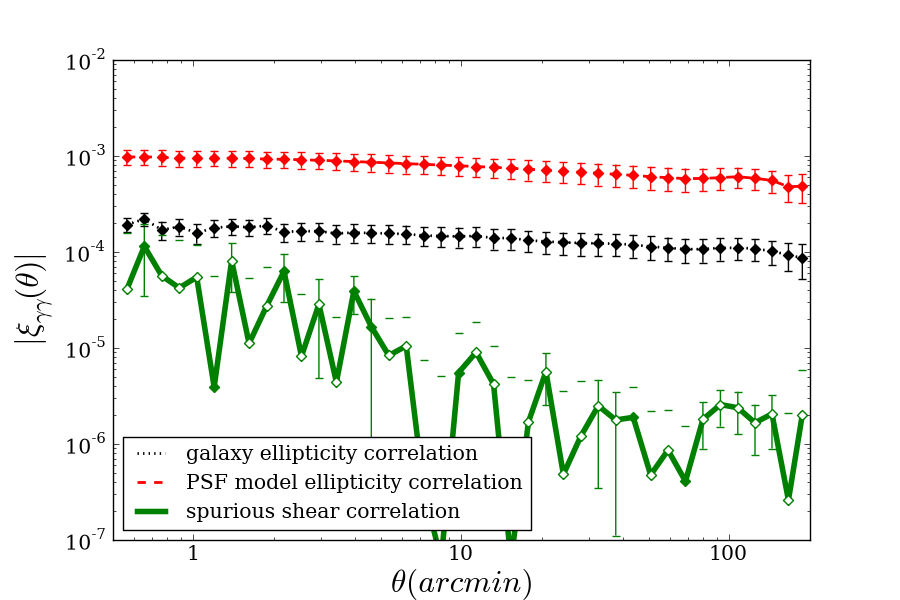
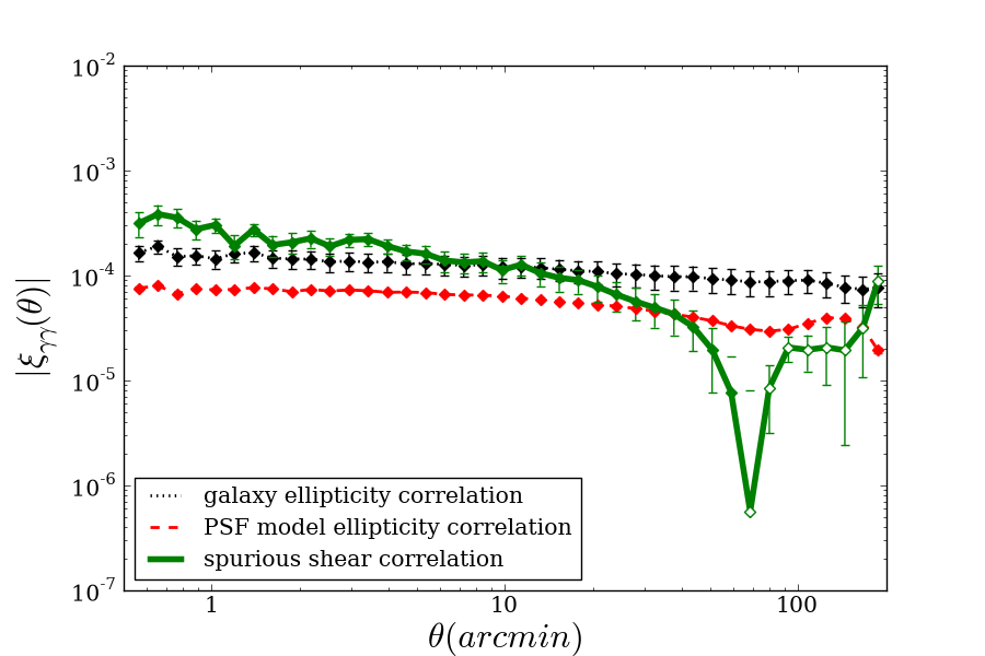
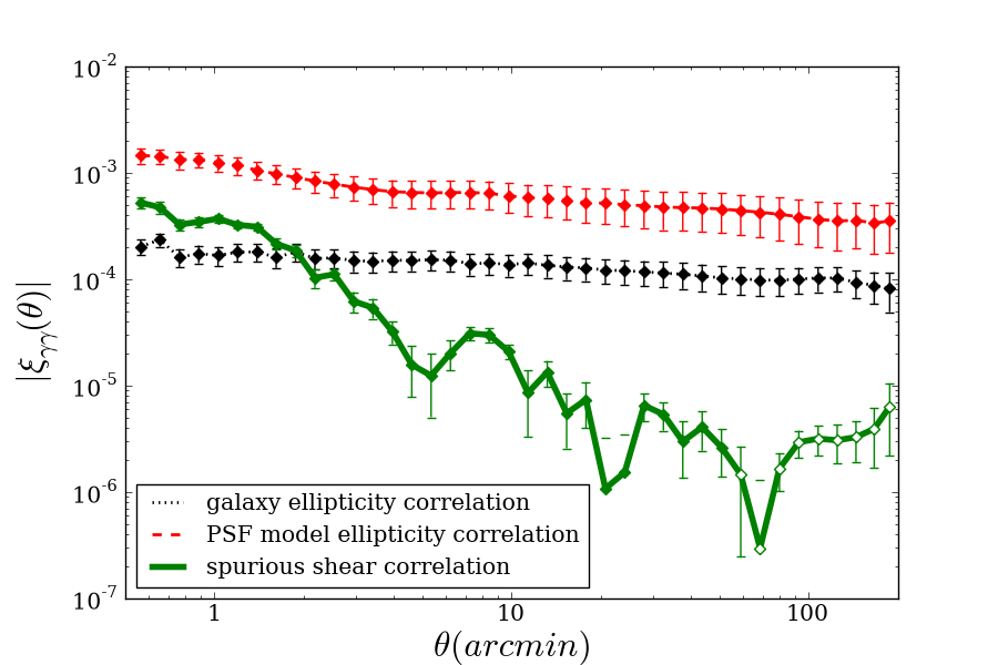
Figure 8: The absolute ellipticity correlation function for the fiducial galaxies before PSF correction (dotted black) and the absolute shear correlation function after PSF correction (solid green) for (a) perfect PSF models, (b) perfect non-stochastic PSF models, and (c) PSF models constructed with a 5th-order polynomial fit to bright stars. The absolute ellipticity correlation function (dashed red) in each case is plotted for comparison. All curves are the medians of 20 different realisations under the fiducial observing condition, with the error bars indicating the standard deviation in the 20 curves divided by $\sqrt{20}$. Negative values are plotted with open symbols.

8 Discussion

8.1 Combining multiple exposures

We now estimate the spurious shear correlation function in a combined 10-year LSST dataset. In the most simplistic case where all $N$ exposures on the same galaxy field have similar image quality, we show in Appendix C that averaging the shear measurements in the $N$ exposures suppresses the stochastic piece of the spurious shear correlation by a factor $N$. But in a realistic case of varying image quality, the $N$ scaling is no longer straightforward. One needs to estimate the “effective number of exposures”, or $N_{\rm eff}$, taken on each galaxy, which essentially weights each exposure according to the image quality. We direct the reader to Appendix D for how we estimated the value of $N_{\rm eff}$ that is suitable for our analysis. From Appendix D, we estimate $N_{\rm eff}$ to be between 184 and 368, with $N_{\rm eff}=184$ being the most pessimistic scenario and $N_{\rm eff}=368$ being the most optimistic.

Consider now the three scenarios described in Section 7, where KSB is used to correct for the PSF effects and the three levels of PSF modelling are assumed. For a hypothetical perfect PSF modelling technique, the shear errors in individual frames are already consistent with zero, so there is no need to discuss the combined results here.

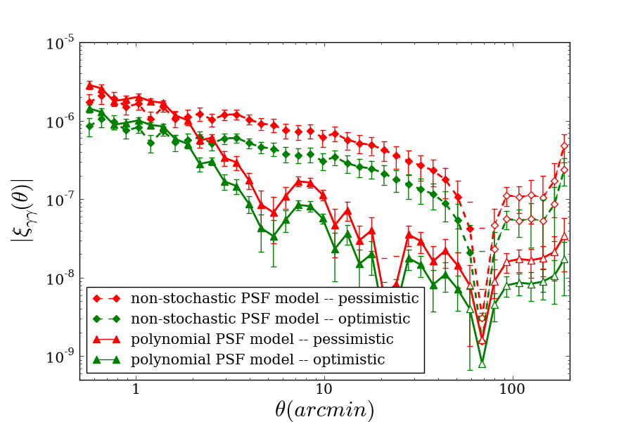
Figure 9: Absolute spurious shear correlation function after combining 10 years of $r$- and $i$-band LSST data when a standard KSB algorithm is implemented and the PSF is modeled at different levels: non-stochastic PSF knowledge only (dashed) and partial stochastic PSF knowledge from polynomial interpolation of stars (solid). Red lines indicate the pessimistic case assuming $N_{\rm eff}=184$ while the green lines show the optimistic case when $N_{\rm eff}=368$ is assumed. All curves are the medians of 20 different realisations under the fiducial observing condition, with the error bars indicating the standard deviation in the 20 curves divided by $\sqrt{20}$. Negative values are plotted with open symbols.

For the second case, we know only the non-stochastic component of the PSF. In this case, spurious shear correlations result from not modelling any of the stochastic component of the PSF shape. In the combined dataset, the latter contribution can be estimated by taking the solid spurious shear correlation function in Figure 8 (b) and multiply by $1/N_{\rm eff}$ to account for the averaging of the stochastic spurious shear correlation.

When both the non-stochastic and stochastic PSF components are modeled using a 5th-order polynomial model fitted to the stars, we assume that the smoothly varying non-stochastic PSF component is fully modeled and the spurious shear is mainly due to stochastic PSF modelling errors. The combined shear correlation function then can be estimated by scaling the spurious shear correlation function in Figure 8 (c) by $1/N_{\rm eff}$.

The total expected spurious shear correlation functions from combining $N_{\rm eff}$ exposures for the latter two cases are shown in Figure 9.

8.2 Implication for constraints on cosmological parameters

We now interpret the spurious shear correlation function derived in Section 8.1 in terms of the implied uncertainties on inferred cosmological parameters.

Since $\boldsymbol{\gamma}=0$ in all our analyses, we can identify the $\xi_{\gamma\gamma}$ measured in Section 7 to be the “additive spurious shear correlation function” $\xi^{s}_{add}$ introduced in Huterer et al. (2006). According to AR08, for several hypothetical forms of the spurious shear power spectrum, one can calculate the upper limits for allowed systematic errors of predictions of the major cosmological parameters via a simple extension to the Fisher Matrix formalism. This upper limits on the systematic errors are set so that the systematic errors do not exceed the statistical errors. In a survey with statistical power similar to the LSST survey, AR08 suggests the following limits on the spurious shear power spectrum:

$$\sigma^{2}_{sys}=\frac{1}{2\pi}\int_{\ell_{min}}^{\ell_{max}}|C^{s}_{add}(\ell)|(\ell+1)d\ell\leq 3\times 10^{-7}\;,$$ (19)

where $C^{s}_{add}$ is the power spectrum corresponding to $\xi^{s}_{add}$, which can be derived through Equation 5.

Equation 19 is in the form of shear power spectra, but our measurements are in the form of shear correlation functions. To properly connect our results to Equation 19, we revisit the hypothetical power spectrum used in AR08:

$$C^{s}_{add}(\ell)=\frac{A_{0}}{\ell(\ell+1)}(n\>\log_{10}(\frac{\ell}{\ell_{0}})+1)\;,$$ (20)

where $n$ is the slope of the log-linear power spectrum, $\ell_{0}$ is an arbitrary reference point chosen to be 700 in the paper and $A_{0}$ is the normalisation.

Since the analytical form of Equation 20 is straightforward to integrate, we can use Equation 5 to find the correlation functions that correspond to power spectra in the form of Equation 20 for a range of $n$ and $A_{0}$ values. These correlation functions then can be compared to the spurious shear correlation functions in Figure 9 to determine the best matched $n$ and $A_{0}$ values. We calculate for this particular set of $n$ and $A_{0}$, the $\sigma^{2}_{sys}$ values and compare with the target set via Equation 19. This process gives us an estimate of the level of uncertainties in the cosmological parameters when these forms of systematic errors in the shear correlation function are present. A more accurate estimate of $\sigma^{2}_{sys}$ can be obtained by the full Fisher Matrix calculation using these measured shear correlation functions.

We explore the parameter space $-3\leq n\leq 1$ and $10^{-9}\leq A_{0}\leq 10^{-5}$, which is chosen to be consistent with the ranges tested in AR08. In this range, we find that the family of functions is not always a good description for the spurious shear correlation function we measure from simulations. In particular, the sharp rising curve and the oscillations at small scales when polynomial PSF models are used cannot be properly modeled by the correlation function corresponding to the log-linear power spectra. As a result, we match scales only larger than $\sim 3^{\prime}$, knowing that in reality these smaller scales ( $<3^{\prime}$) may not enter in constraining cosmology. The resulting $n$ and $A_{0}$ values as well as the corresponding $\sigma^{2}_{sys}$ values are listed in Table 4. Figure 10 shows, for the optimistic case, the two spurious shear correlation functions overlaid by their functional-form counter parts. Note that these grey curves are not fits – they are matched visually because the shapes of the measured shear correlation functions are quite different from the assumed functional forms.

Table 4: For the 10-year combined $r$- and $i$-band data of LSST, the best matched $n$’s and $A_{0}$’s to the spurious shear correlation function under different scenarios are listed. The numbers are measured with a KSB pipeline and under two different PSF model assumptions. Two scenarios for effective number of exposures for each field are assumed: the optimistic case corresponds to $N_{\rm eff}=368$ and the pessimistic case corresponds to $N_{\rm eff}=184$.

PSF model	$N_{\rm eff}$	$n$	$\log_{10}(A_{0})$	$\sigma^{2}_{sys}$
Non-stochastic	optimistic	0.7	$-5.7$	2.17$\times 10^{-6}$
	pessimistic		$-5.4$	4.34$\times 10^{-6}$
Polynomial	optimistic	0.7	$-6.6$	2.74$\times 10^{-7}$
	pessimistic		$-6.3$	5.46$\times 10^{-7}$

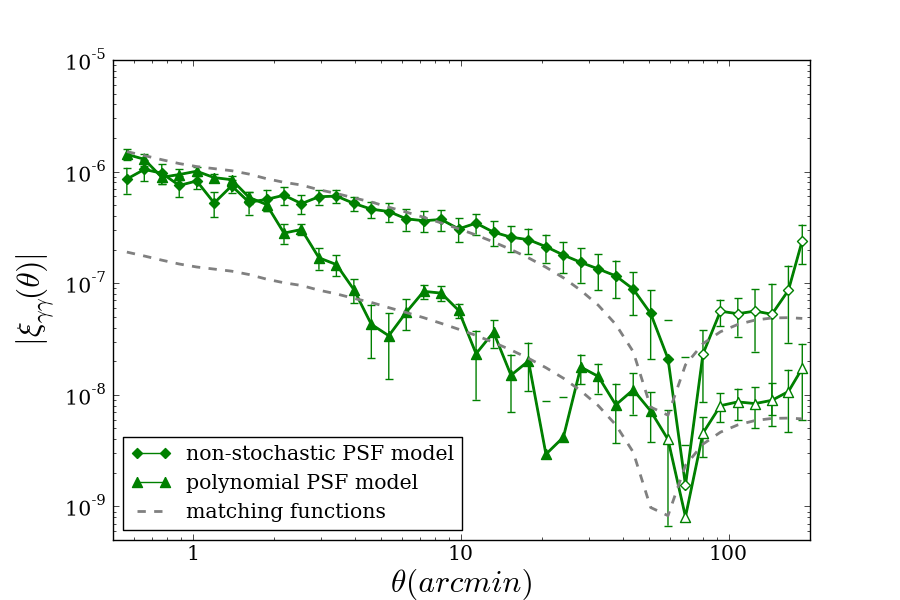
Figure 10: The two spurious shear correlation functions in the optimistic scenario (solid green) overlaid with functional forms assumed by AR08 that visually match the level and approximate shapes of the spurious shear correlation (dashed grey). The green curves are the medians of 20 different realisations under the fiducial observing condition, with the error bars indicating the standard deviation in the 20 curves divided by $\sqrt{20}$. Negative values are plotted with open symbols.

In Table 4 we show that in the canonical weak lensing pipeline (KSB + polynomial PSF model), the spurious shear power spectrum we have measured from simulations is approximately 0.9 – 1.8 times the statistical errors. Although the numbers imply that by using the current weak lensing pipeline, we are already reaching the level of systematics in shear measurements required for LSST, it should be understood that not all potential effects (such as shear calibration, galaxy modeling, photo-z estimation, chromatic PSF effect etc.) have yet been included. To ensure that the cosmic shear measurements from LSST is not systematics-limited after considering all the other systematic errors, we will need shear measurement methods more sophisticated than what we used in this study.

We can trace the source of these systematic errors to improper modelling of the stochastic PSF using polynomial functions, which needs to be reduced when developing the next generation of shear measurement algorithms. On the other hand, if only the non-stochastic errors are modeled, the spurious shear due to not modelling the stochastic PSF results in a $\sigma^{2}_{sys}$ value one order of magnitude greater than the target value. This implies that the stochastic PSF components do not average out enough by themselves if not corrected, even when the full dataset is combined. We thus show the importance of modelling the stochastic as well as the non-stochastic components of the PSF.

We have shown here that given a typical weak lensing pipeline, the major physical effects in an LSST observation will not seriously limit LSST, provided that the number of exposures in the combined dataset and the image quality are as expected.

8.3 Effect of simplifications

At this point we summarize the major assumptions that underlie our analysis to provide context for our results:

First, we have deliberately designed our simulations and the analysis we performed to minimize algorithm-dependent contributions to the errors. In particular, we used circular Gaussians as our galaxy models, invoked KSB as our shear measurement method, and performed an artificial “perfect calibration” for the KSB pipeline. Thus the results derived in Sections 8.1 and 8.2 only take account of the algorithm-independent part of the additive spurious shear correlation function. In particular, recent work (Hirata & Seljak, 2003; Réfrégier et al., 2012; Melchior & Viola, 2012) has shown that the algorithm-dependent shear errors are strongly affected by noise (the so called “noise bias”), which arises from using very low SNR galaxies. In our analyses, this factor is suppressed through the use of a simplistic galaxy model. However, given the low SNR ($\sim$8) of our fiducial galaxy, the noise bias for realistic weak lensing galaxies may not be negligible.

Second, we have not taken into account more sophisticated schemes for combining shear measurements from multiple exposures. As suggested by Jain et al. (2006), the stochastic component in the shear errors can be eliminated by dividing the full dataset into sub-groups of exposures and only correlating shear measurements between different sub-groups. We provide a brief discussion in Appendix E of such implementations, but have not investigated the full power of these alternative approaches in this paper.

Third, as mentioned in Section 1, this work is based on the projected two-point shear correlation function. In a full weak lensing analyses where lensing tomography and higher-order statistics are used, additional constraints may arise. However, the combination of all these different statistics may also be useful in mitigating certain systematic effects.

Finally, we also note that the applicability of the extended Fisher Matrix formulae in AR08 and therefore Equation 19 to our analyses depends on some specific assumptions regarding the statistical properties of the spurious shear contributions we measure in the simulations. The main assumption in AR08 is that the higher-order statistical properties of the spurious shear are similar to those of the true shear – a Gaussian random field – so that the covariance matrix for the spurious shear power spectrum is close to diagonal. (This is implicitly assumed when deriving Equation 10 from Equation 9 in AR08.) Since the statistical properties of the spurious shear depend on its physical origin, they are not guaranteed to be Gaussian. However, in our simulations, the effect of such non-Gaussian spurious shear is likely to be small compared to the Gaussian component generated from counting statistics and the various stochastic effects; therefore the results derived in Section 8.2 should be sufficiently robust.

9 Conclusions

In this paper, we have carried out a bottom-up, quantitative study of the potential systematic errors in cosmic shear measurements for future LSST-like surveys using high fidelity simulations.

Simulations are generated using PhoSim, a photon-by-photon Monte Carlo ray-tracing software that models all major physical effects from the top of the atmosphere down through the detectors. Specifically, we have generated a suite of special simulations in order to isolate the systematic errors in ellipticity and shear measurements caused by different physical effects, which would have been impossible to achieve with a real telescope.

We identify the most important physical effects in terms of their impact on ellipticity measurements and classify them into two classes: non-stochastic and stochastic. The ellipticity errors and their correlation properties caused by each individual effect are then quantified in a systematic way. We find that, in a single LSST exposure:

• Ellipticity errors due to counting statistics dominate the total ellipticity errors, whereas ellipticity errors due to atmospheric and instrumental effects dominate the total ellipticity error correlation function.

• The ellipticity error correlation function due to non-stochastic effects is one order of magnitude smaller than that due to stochastic effects.

For shear measurement, we identify three steps in a canonical weak lensing pipeline that lead to spurious shear, two of which are dominated by the specific algorithm chosen for PSF characterisation and deconvolution, which we have not investigated in detail. The third step involves modelling the PSF spatial variation with scattered stars. We carry out the full analyses with a standard weak lensing algorithm and quantify the spurious shear correlation under different assumptions about the PSF model. We draw several conclusions:

• With perfect PSF knowledge, systematics induced by the algorithm in an idealised KSB implementation are negligible.

• Not correcting for the stochastic component of the PSF shape introduces large shear systematics in the correlation function.

• A conventional PSF modelling scheme using polynomial interpolation of stars can partially model the stochastic PSF contribution, but the inflexibility of the functional form of polynomials limits the power of this method.

The single-exposure results are then extrapolated to the full combined 10-year dataset, and finally interpreted in terms of the constraints on dark energy parameters according to an extended Fisher Matrix calculation from AR08. We draw several conclusions:

• By using a canonical weak lensing analysis pipeline, the systematic errors in the spurious shear correlation function induced by the major physical effects, after combining the 10 years of LSST data, is at a level approaching the statistical errors.

• The errors mainly come from imperfect modelling of the stochastic PSF, which has not been studied in detail in the past. This calls for better basis functions that can characterise structures in the stochastic PSF variation on all scales.

Finally, this analysis is done under several assumptions and simplifications, which may need to be taken into account when interpreting the results:

• We have designed the simulations and analysis to avoid algorithm-dependence of this analysis. Algorithm errors will need to be estimated and combined with the results here to yield the total shear systematic errors.

• A simple scheme is used for combination of shear measurements in multiple exposures. More intelligent use of the data can potentially give better results.

• Only a projected 2D two-point correlation function is analysed. By implementing weak lensing tomography or higher-order statistics, some of the spurious shear can be mitigated.

• We adopt the results from AR08 to interpret the spurious shear correlation function in terms of its effect on the uncertainty in predicting cosmological parameters, which implicitly assume that the spurious shear has statistical properties similar to the true shear.

Appendix A Physical models in PHOSIM

A.1 Optics and optics perturbations

PhoSim builds in the most up-to-date optics design of the instrument. This includes detailed specifications of the dimensions and wavelength response of each optical element from the engineering design (the three mirrors, three lenses and the filter), characteristics of the backside-illuminated thick CCD detectors, and other telescope components such as the shutter and spider, scattered light and tracking mechanisms. The PhoSim version used in this paper is based upon the optics baseline design version 3.3.

In addition to the design, PhoSim also models the level of residual wavefront errors after a typical correction from the AOS has been made. The effects of these residuals are modeled using hundreds of parameters that displace or deform the different optical components, causing the PSF to degrade from the design within levels allowed by the engineering requirements on the AOS. This approach is different from an exact simulation of the AOS, which would have to take into account the history of the wavefront measurements over a period of hours as the survey proceeds. The latter approach would require a vast increase in the number of exposure simulations that are performed, and is thus computationally impractical. Therefore, the current PhoSim takes the alternative approach of modelling residuals of the full control loop instead. Since exposures on the same patch of sky are usually separated by a few days, which is much longer than a typical time scale for the AOS updates, the assumptions involved in this procedure are well justified.

We further classify the residual wavefront errors, or optics errors in PhoSim, into two classes. The first class accounts for errors that originate from fabrication and integration, or are introduced by gravity and the thermal environment of the telescope. The former are permanent functions of the response, while the latter are by nature highly repeatable, and the zeroth-order corrections will be implemented by the AOS according to a pre-calibrated look-up table. However, the AOS cannot perfectly compensate for all distortions given the limited number of degrees of freedom that are actively controlled; therefore, there will be repeatable optics errors, which are “non-stochastic”. The characteristic amplitudes of these perturbations used in PhoSim are derived from finite element modelling of the telescope and camera under appropriate gravity and thermal loads. The second class includes the residual wavefront errors as well as actuator errors and wind shake. Since these effects are random in nature and do not show repeated patterns across exposures, they can be measured only by monitoring the wavefront errors in real time. The imperfect correction by the AOS for these effects introduces “stochastic” optics errors which are uncorrelated from exposure to exposure. For the purpose of this paper, we deliberately implement the optics model in PhoSim in a way that allows the two classes of optics errors to be separated – this is because we are interested in how they separately enter into the shear measurements, as discussed in more detail in Section 4.

The typical levels of the two classes of optics errors on the major optical elements used in this analysis are listed in Table 5. Note that the numbers corresponding to this classification scheme are based on the current engineering specifications (Ivezic et al., 2011, and internal documents), but the results are easily scalable if different specifications are eventually adopted..

Table 5: Specifications of the major optics errors modeled in PhoSim. We describe the surface height variations on the mirrors using 2nd- through 5th- order Zernike polynomials, where each polynomial is normalised individually with some amplitude according to typical values observed in existing systems. We list here only the range for the four amplitudes used.

Source of error	Stochastic or not	Random sampling	Physical parameter	RMS values
	non-stochastic	Gaussian	misalignment	$1.08\times 10^{-2}$ (mm)
Solid-body optics errors			tip/tilt	$2.34\times 10^{-6}$ (rad)
in the mirrors	stochastic	Gaussian	misalignment	$1.89\times 10^{-2}$ (mm)
			tip/tilt	$4.09\times 10^{-6}$ (rad)
Surface height variation	non-stochastic	Gaussian	coefficients of Zernike	(0.38 – 2.20) $\times 10^{-4}$ (mm)
in the mirrors	stochastic		polynomial expansion	(0.76 – 4.40) $\times 10^{-4}$ (mm)
	non-stochastic	Gaussian	misalignment	$3.24\times 10^{-2}$ (mm)
Solid-body optics errors			tip/tilt	$1.58\times 10^{-4}$ (rad)
in the camera	stochastic	Gaussian	misalignment	$5.67\times 10^{-2}$ (mm)
			tip/tilt	$3.77\times 10^{-4}$ (rad)
Sensor surface displacement	non-stochastic	Zernike expansion based	height	5$\times 10^{-3}$ (mm)
from ideal focal plane		on laboratory measurements	variation

A.2 Tracking errors

Tracking errors in PhoSim are modeled by a Gaussian random walk of the telescope pointing in each of the three directions: azimuth, elevation and rotation, where a step is taken every 0.1 second throughout the exposure. The effect of the tracking error integrated over 15 seconds is to yield a root-mean-squared (RMS) error of $\sim 0.02$" in the azimuth and elevation directions, and $\sim 1$" in rotation.

A.3 The atmospheric model

Due to the short exposure time of LSST, atmospheric effects on image distortions become more pronounced in a single exposure than what is usually seen in longer exposures. Since these atmosphere-induced distortions arise from turbulent structures in the air density, we can also expect spatial structures in the image shape distortions across the field which are associated with the turbulent structures. De Vries et al. (2007) first showed via simulations that the effect of the atmospheric turbulence on PSF shape distortion averages out rapidly with exposure time, while Wittman (2005) and Heymans et al. (2012) measured the correlation of PSF shape distortions in short exposure data and discuss their potential effect on weak lensing.

Similar to the pure atmospheric simulations in De Vries et al. (2007), the atmosphere in PhoSim is modeled by multiple layers of moving atmospheric screens. The “frozen screen approximation” is justified since the time scale for the shapes of turbulent cells to change significantly is much longer than the time required for turbulence cells to pass through the field of view, given the typical wind speeds of a few meters per second (Taylor, 1938; Poyneer et al., 2009).

The heart of the atmospheric model is a set of multi-scale, multi-layer frozen Kolmogorov screens (Kolmogorov, 1992). These atmospheric screens are constructed according to a full 3D Kolmogorov spectrum with assigned parameters including the structure function, inner scale, outer scale, wind speed and wind direction. All parameters are modeled from existing atmospheric data taken near the LSST site. In Peterson et al. (2012), we explain the theoretical justification of the approach we have taken, as well as the major innovations in the PhoSim atmospheric model.

Appendix B KSB formulas

The following formulas are the foundation for performing a weak lensing measurement using the KSB algorithm. We use the Einstein summation convention.

First, stars and galaxies are measured with the “getshape” imcat routine, which assigns to each object the following shape parameters: the complex ellipticity ($\varepsilon_{\alpha}$), the smear polarisability ($P^{sm}_{\alpha\beta}$) and the shear polarisability ($P^{sh}_{\alpha\beta}$), where $\alpha,\beta=1,2$. $\varepsilon_{\alpha}$ is defined in Equations 1 and 2, while $P^{sm}_{\alpha\beta}$ and $P^{sh}_{\alpha\beta}$ are calculated through

$$P_{\alpha\beta}^{sm}=X_{\alpha\beta}^{sm}-\varepsilon_{\alpha}\varepsilon_{\beta}^{sm}\;,$$ (21)

$$P_{\alpha\beta}^{sh}=X_{\alpha\beta}^{sh}-\varepsilon_{\alpha}\varepsilon_{\beta}^{sh}\;.$$ (22)

$X_{\alpha\beta}^{sm}$, $X_{\alpha\beta}^{sh}$, $\varepsilon_{\beta}^{sm}$ and $\varepsilon_{\beta}^{sh}$ are derived through combinations of weighted second moments of the light profile of the object $f(x_{1},x_{2})$ and derivatives of the weighting function $W(x_{1},x_{2})$ (see Kaiser et al., 1995, for definitions of these quantities). Each component $\varepsilon_{\alpha}$, $P^{sm}_{\alpha\beta}$ and $P^{sh}_{\alpha\beta}$ for the stars is interpolated to the galaxys’ locations and recalculated with the galaxys’ weighting functions. The remeasured quantities will be used to construct the PSF model for the galaxy.

The anisotropic PSF effects on the galaxy’s ellipticity are first corrected through

$$\delta\varepsilon_{\alpha}=P_{\alpha\beta}^{sm}p_{\beta}\;,$$ (23)

where

$$p_{\alpha}=(P^{*,sm})^{-1}_{\alpha\beta}\varepsilon^{*}_{\beta}\;.$$ (24)

The superscript “$*$” indicates parameters of the PSF model. Shear $g_{\alpha}$ changes the galaxy’s ellipticity by

$$\delta\varepsilon_{\alpha}=P_{\alpha\beta}^{sh}g_{\beta}\;.$$ (25)

Finally, we need to correct for the weighting and circular seeing effects to get the final shear estimate for each galaxy by replacing $P_{\alpha\beta}^{sh}$ with the shear susceptibility $P_{\alpha\beta}^{\gamma}$, where

$$P_{\alpha\beta}^{\gamma}=P^{sh}_{\alpha\beta}-P^{sm}_{\alpha\gamma}(P^{*,sm})^{-1}_{\gamma\delta}P^{*,sh}_{\delta\beta}\;.$$ (26)

$P_{\alpha\beta}^{\gamma}$ is eventually replaced by $\frac{1}{2}tr[P^{\gamma}]$ in our approach, similar to the “ES2” method in Massey et al. (2007).

Appendix C $1/N$ scaling for the stochastic spurious shear correlation

To demonstrate the $1/N$ scaling for the stochastic spurious shear correlation, we use the 20 simulated shear catalogues used in Section 7.3, where we have argued that most of the shear errors in these catalogues are stochastic. We then consider averaging shear measurements of the same galaxy in the first $N$ different frames, and calculate the shear correlation function for the averaged shear catalogue as a function of $N$.

The results for $N=1,5,20$ are shown in Figure 11. We observe that, although the low statistics causes the data to be quite noisy, the spurious shear correlation function does roughly follow the $1/N$ scaling. This supports our argument in Section 8.1, where we extrapolate our single-exposure measurements to the full 10-year LSST dataset.

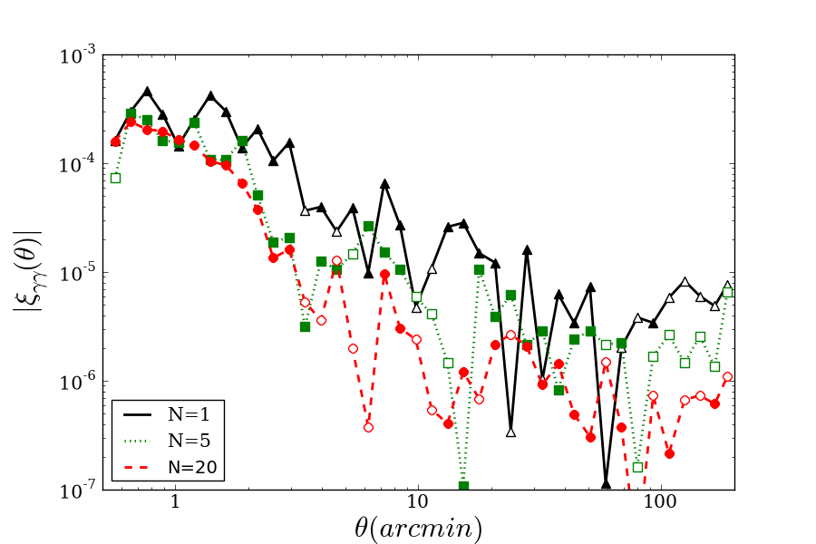
Figure 11: The spurious shear correlation function for the mean shear catalogue for $N$ exposures, where $N=1$ (solid black), 5 (dotted green) and 20 (dashed red). The shear catalogue is obtained via standard KSB algorithm and 5th-order polynomial PSF models. Negative values are plotted with open symbols.

Appendix D Effective number of exposures

In the 10-year period of observation planned for LSST, every patch of sky is imaged approximately 386 times, each with 15-second exposures (the number doubles to 772 if $r$ and $i$ bands are combined); however, because of variation in the observing conditions and the galaxy properties themselves, not all galaxies have good shape measurements in all exposures. The power of combining a multi-epoch dataset is that one has the freedom to weight the contributions of a single galaxy shape measurement in each of the different exposures according to the image quality, and thus extract the maximum information from the noisy dataset. This effectively means that the “stochastic” spurious shear correlation will not cancel as fast as $1/772$ under this framework, because some of the exposures will be down-weighted due to their poor image quality. Instead, the spurious shear correlation will decrease only as fast as $1/N_{\rm eff}$, where $N_{\rm eff}$ is the “effective number of exposures” for the entire dataset. $N_{\rm eff}$ depends on the detailed distribution of the observing conditions, the galaxy distributions (brightness, size, redshift), as well as the analysis pipeline used. The precise determination of $N_{\rm eff}$ is complicated and beyond the scope of this paper; however, we can provide optimistic and pessimistic estimates for $N_{\rm eff}$ to bound the final results in a reasonable range.

In this work, we have chosen the fiducial observing conditions (Table 1) to correspond to roughly the median condition of the best 50% of the dataset in terms of image quality. This gives approximately 184 exposures in the $r$ band as well as the $i$ band, or $\sim$368 exposures for the entire weak lensing dataset for each field. We view this as an optimistic estimation, since it has been shown (Hirata & Seljak, 2003; Réfrégier et al., 2012; Melchior & Viola, 2012) that for PSF sizes approaching the size of average galaxies (for part of the 368 exposures), the systematics can grow nonlinearly and the median spurious shear of these 368 exposures can be larger than that shown in Figure 8. Furthermore, as mentioned in Section 4.1, errors in the 2 exposures in the same visit may be correlated, effectively lowering $N_{\rm eff}$ for the full dataset. A more conservative estimation is to use only the best 25% of the exposures to make cosmic shear measurements. In this case we have a total of 184 exposures and the results are likely to be pessimistic, since the median spurious shear correlation of these 184 exposures is likely to be better than those measured in Figure 8. We can assume that the optimal outcome of combining the full 10-year data lies in between these two bounds $N_{\rm eff}=184$ and $N_{\rm eff}=368$.

Appendix E Correlating shear measurements across exposures

In addition to the simple averaging scheme discussed in Section 8.1, previous papers (see e.g.  Jain et al., 2006) also have suggested correlating galaxies in different exposures to eliminate the stochastic systematics in the atmosphere and instrument. In theory, by correlating shear measurements across exposures, only the non-stochastic systematics remain, which do not scale down further with number of exposures. This, however, comes with the price of decreasing the statistical power of a dataset, since there will be a smaller number of pairs that contribute to the correlation function. The statistical errors are increased by $\sqrt{N_{\rm eff}/(N_{\rm eff}-1)}$.

For LSST, the full 10-year dataset includes $N_{\rm eff}=$184 – 368, which means that implementing cross correlation will not degrade the statistical power significantly. However, at earlier stages of the survey, when $N_{\rm eff}$ is still small, the $\sqrt{N_{\rm eff}/(N_{\rm eff}-1)}$ penalty may overcome the benefit of implementing cross correlation. For the purpose of this paper, we will not discuss the details of optimising the combined multi-epoch dataset; rather, we show one simple example for implementation of cross correlation and merely demonstrate an alternative way of combining multiple exposures to improve upon our results.

For the 20 simulations in the master set in Section 7, we take the spurious shear obtained from the 5th-order polynomial PSF models and calculate 10 correlation functions by correlating shear measurements for galaxies in two different exposures (the 20 exposures were split into 10 groups of image pairs, for which the shear measurement in each image is correlated only with shear measurements in the other image). The median of the 10 correlation functions is plotted in Figure 12, together with the shear correlation functions in Figure 8, scaled to $N_{\rm eff}=2$, so that all curves represent the spurious shear correlation function for combining a dataset of two independent exposures. Note that in Figure 12, the shear correlation function from correlating galaxies in different exposures is essentially consistent with zero at angular scales larger than $\sim 3^{\prime}$, but rises steeply smaller angular scales. This may be because the PSF models are consistently ill behaved on the edges of the CCD sensors from the polynomial PSF model, making some of the PSF model errors “non-stochastic” between frames. This is likely to be an unrealistic artifact since no rotation/dithering is used in the 20 images.

This suggests that correlating galaxies across different exposures can suppress some of the stochastic systematics. But similar to the auto-correlation technique, the calculation depends on a good PSF modelling process that does not create artificial non-stochastic errors. Given the loss of statistical power by correlating across exposures, a more detailed investigation of these tradeoffs will be needed to establish the optimal use of LSST’s multi-epoch dataset.

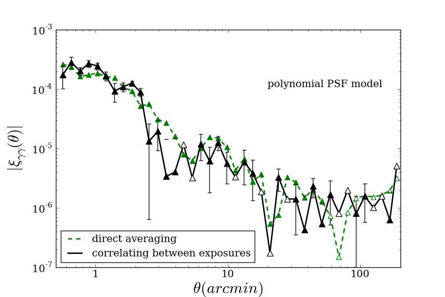
Figure 12: For two typical LSST exposures combined, the spurious shear correlation function when a standard KSB algorithm is implemented with 5th-order polynomial PSF models and only galaxies from different exposures are correlated (black). Compared with the simple average scheme (dashed green), correlating galaxies from different exposures suppresses mainly spurious shear correlation on large scales. The error bars for the black curve indicate the standard deviation in the 10 curves divided by $\sqrt{10}$. Negative values are plotted with open symbols.

References

- Albrecht et al. (2006) Albrecht A., et al., 2006, APS April Meeting Abstracts, pp G1002+
- Amara & Réfrégier (2007) Amara A., Réfrégier A., 2007, MNRAS, 381, 1018
- Amara & Réfrégier (2008) Amara A., Réfrégier A., 2008, MNRAS, 391, 228
- Bacon et al. (2000) Bacon D. J., Réfrégier A. R., Ellis R. S., 2000, MNRAS, 318, 625
- Bartelmann & Schneider (2001) Bartelmann M., Schneider P., 2001, Physics Reports, 340, 291
- Benjamin et al. (2007) Benjamin J., et al., 2007, MNRAS, 381, 702
- Bertin & Arnouts (1996) Bertin E., Arnouts S., 1996, A&AS, 117, 393
- Bridle et al. (2010) Bridle S., et al., 2010, MNRAS, 405, 2044
- Chang et al. (2012) Chang C., et al., 2012, in preparation
- Connolly et al. (2010) Connolly A. J., et al., 2010, in SPIE Conference Series Vol. 7738 of SPIE Conference Series, Simulating the LSST system
- De Vries et al. (2007) De Vries W. H., et al., 2007, ApJ, 662, 744
- Hetterscheidt et al. (2007) Hetterscheidt M., et al., 2007, A&A, 468, 859
- Heymans et al. (2006) Heymans C., et al., 2006, MNRAS, 368, 1323
- Heymans et al. (2012) Heymans C., et al., 2012, MNRAS, 421, 381
- Hirata & Seljak (2003) Hirata C., Seljak U., 2003, MNRAS, 343, 459
- Hoekstra et al. (1998) Hoekstra H., et al., 1998, ApJ, 504, 636
- Hoekstra et al. (2006) Hoekstra H., Mellier Y., van Waerbeke L., Semboloni E., Fu L., Hudson M. J., Parker L. C., Tereno I., Benabed K., 2006, ApJ, 647, 116
- Hu (1999) Hu W., 1999, ApJ, 522, L21
- Hu & Tegmark (1999) Hu W., Tegmark M., 1999, ApJ, 514, L65
- Huff et al. (2011) Huff E. M., et al., 2011, ArXiv e-prints
- Huterer et al. (2006) Huterer D., Takada M., Bernstein G., Jain B., 2006, MNRAS, 366, 101
- Ivezic et al. (2008) Ivezic Z., et al., 2008, ArXiv e-prints: astro-ph/0805.2366
- Ivezic et al. (2011) Ivezic Z., et al., 2011, The LSST System Science Requirement Document v5.2.3
- Jain et al. (2006) Jain B., Jarvis M., Bernstein G., 2006, Journal of Cosmology and Astroparticle Physics, 2, 1
- Jain & Seljak (1997) Jain B., Seljak U., 1997, ApJ, 484, 560
- Jarvis & Jain (2004) Jarvis M., Jain B., 2004, ArXiv e-prints: astro-ph/0412234
- Jarvis et al. (2008) Jarvis M., Schechter P., Jain B., 2008, ArXiv e-prints: astro-ph/0810.0027
- Jee & Tyson (2011) Jee M. J., Tyson J. A., 2011, PASP, 123, 596
- Kaiser (1998) Kaiser N., 1998, ApJ, 498, 26
- Kaiser et al. (1995) Kaiser N., Squires G., Broadhurst T., 1995, ApJ, 449, 460
- Kaiser et al. (2000) Kaiser N., Wilson G., Luppino G. A., 2000, ArXiv e-prints: astro-ph/0003338
- Kitching et al. (2012a) Kitching T. D., et al., 2012a, MNRAS, 423, 3163
- Kitching et al. (2012b) Kitching T. D., et al., 2012b, ArXiv e-prints: astro-ph/1204.4096
- Kolmogorov (1992) Kolmogorov A., 1992, Dokl. Akad. Nauk SSSR, 30, 301
- Krabbendam et al. (2010) Krabbendam V., et al., 2010, in AAS Meeting Abstracts #215 Vol. 42 of Bulletin of the AAS, LSST Operations Simulator. pp 401.05–+
- Lin et al. (2011) Lin H., et al., 2011, ArXiv e-prints
- Luppino & Kaiser (1997) Luppino G. A., Kaiser N., 1997, ApJ, 475, 20
- Massey et al. (2007) Massey R., et al., 2007, MNRAS, 376, 13
- Melchior & Viola (2012) Melchior P., Viola M., 2012, MNRAS, p. 3383
- Paulin-Henriksson et al. (2008) Paulin-Henriksson S., Amara A., Voigt L., Réfrégier A., Bridle S. L., 2008, A&A, 484, 67
- Peterson et al. (2009) Peterson J. R., et al., 2009, LSST Science Book, Version 2.0, Chapter 3.3
- Peterson et al. (2012) Peterson J. R., et al., 2012, in preparation
- Poyneer et al. (2009) Poyneer L., van Dam M., Véran J.-P., 2009, Journal of the Optical Society of America A, 26, 833
- Réfrégier et al. (2012) Réfrégier A., et al., 2012, ArXiv e-prints
- Schneider et al. (2005) Schneider P., Kilbinger M., Lombardi M., 2005, A&A, 431, 9
- Schneider & Lombardi (2003) Schneider P., Lombardi M., 2003, A&A, 397, 809
- Schrabback et al. (2010) Schrabback T., et al., 2010, A&A, 516, A63+
- Semboloni et al. (2006) Semboloni E., et al., 2006, A&A, 452, 51
- Taylor (1938) Taylor G. I., 1938, Royal Society of London Proceedings Series A, 164, 476
- Tyson (2002) Tyson J. A., 2002, in J. A. Tyson & S. Wolff ed., SPIE Conference Series Vol. 4836 of SPIE Conference Series, Large Synoptic Survey Telescope: Overview. pp 10–20
- Wittman (2005) Wittman D., 2005, ApJ, 632, L5
- Wittman et al. (2000) Wittman D. M., et al., 2000, Nature, 405, 143
- Zhang (2010) Zhang J., 2010, MNRAS, 403, 673