Characterization of the X-ray light curve of the $\gamma$ Cas-like B1e star HD 110432

Abstract

HD 110432 (BZ Cru; B1Ve) is the brightest member of a small group of “$\gamma$ Cas analogs” that emit copious hard X-ray flux, punctuated by ubiquitous “flares.” To characterize the X-ray time history of this star, we made a series of six RXTE multi-visit observations in 2010 and an extended observation with the XMM-Newton in 2007. We analyzed these new light curves along with three older XMM-Newton observations from 2002–2003. Distributed over five months, the RXTE observations were designed to search for long X-ray modulations over a few months. These observations indeed suggest the presence of a long cycle with P $\approx$ 226 days and an amplitude of a factor of two. We also used X-ray light curves constructed from XMM-Newton observations to characterize the lifetimes, strengths, and interflare intervals of 1615 flare-like events in the light curves. After accounting for false positive events, we infer the presence of 955 (2002-2003) and 386 (2007) events we identified as flares. Similarly, as a control we measured the same attributes for an additional group of 541 events in XMM-Newton light curves of $\gamma$ Cas, which after a similar correction yielded 517 flares. We found that the flare properties of HD 110432 are mostly similar to our control group. In both cases the distribution of flare strengths are best fit with log-linear relations. Both the slopes of these distributions and the flaring frequencies themselves exhibit modest fluctuations. We discovered that some flares in the hard X-ray band of HD 110432 were weak or unobserved in the soft band and vice versa. The light curves also occasionally show rapid curve drop offs that are sustained for hours. We discuss the existence of the long cycle and these flare properties in the backdrop of two rival scenarios to produce hard X-rays, a magnetic star-disk interaction and the accretion of blobs onto a secondary white dwarf.

1. Introduction: HD110432 among $\gamma$ Cas analogs

For many years $\gamma$ Cas (B0.5e IV) held the title of “odd man out” among X-ray emitting stars because of its peculiar set of X-ray characteristics. These include a moderately elevated L_x (by a factor of 10) compared to X-ray emission of other main sequence B stars and an almost ubiquitous X-ray flaring. The X-ray spectrum is dominated by emission from an optically thin plasma, parameterized by $kT$ $\sim$ 13 keV (Lopes de Oliveira et al. 2010; “L10”). These characteristics are unlike those in X-ray spectra of other massive stars and indicate that an unusual mechanism is at play between the Be star and its local environment.

Recently several members of a new “$\gamma$ Cas class” of X-ray emitters have been discovered with spectral types near B0.5, but one, HD 157832, is classified as late as B1.5e (Lopes de Oliveira & Motch 2011). The first and also brightest of these “analogs” is the B1e star HD 110432 (Smith & Balona 2006; “SB”), also known as BZ Cru. This star is also the object of this study. The remaining seven members of the class are listed in Motch et al. (2007) and Smith et al. (2012; “S12”).

The prototype of this group, $\gamma$ Cas, has a high rotation velocity. Its spectrum exhibits strong H$\alpha$ line emission strength formed in a mass loss disk. The star in actually a binary system with a circular orbit and a P_orb = 203.53 $\pm{0.08}$ days (Nemravová et al. 2012, Smith et al. 2012). Two of the analog members are likely to be blue stragglers in Galactic clusters, although none of them is known yet to be in a binary system. These are USNO 0750-1354972 in NGC 6649 (50 Myr) and HD 119682 in NGC 5281 (40 Myr). Our target, HD 110432, may be a member of NGC 4609 (Feinstein & Marraco 1979). If so, its age is 60 Myr. These ages are about twice the age of B0.5-B1 main sequence stars.

HD 110432 is situated in the sky at the edge of the Coalsack and has a revised Hipparcos distance of 373$\pm{43}$ pc (van Leeuwen 2007). Nonetheless, Rachford et al. (2001) found that the ISM column length toward the star is an equivalent hydrogen column of 1$\times$10²¹ atoms cm^-2. Lopes de Oliveira et al. (2007; “L07”) and Torrejón et al. (2012; “T12”) have fit the fluxes of XMM-Newton, Chandra, and Suzaku high resolution spectra with multi-component, optically thin, thermal models. Their models require a larger absorption column(s) toward the X-ray sources than the UV-derived ISM column, suggesting that cold matter lies in front of them. The T_eff and surface gravity of the star have been estimated from a measurement of its optical Balmer jump (22,510 K, log g = 3.9; Zorec et al. 2005), the strength of the He II 1640 Å line ($\sim$25,000 K; SB), and a fitting of the UV-to-IR spectral energy distribution (25,000 K, log g = 3.5; Codina et al. 1984). Frémat et al. (2005) gave a rotational velocity $vsin\,i$ = 441$\pm{27}$ km s^-1 for $\gamma$ Cas. SB reported that the velocity of HD 110432 is at least 90% of the $\gamma$ Cas value, i.e., $\approx$400 km s^-1. When we consider their intermediate $sin\,i$ values (Stee et al. 2012, SB), the $vsin\,i$’s of HD 110432 and $\gamma$ Cas suggest that these stars rotate at close to their critical values.

Because of its relative proximity to the Sun, HD 110432 has been the object of more studies than other $\gamma$ Cas analogs. The models fitting the X-ray spectra of this star are similar to the four plasma component model found for $\gamma$ Cas (S12). The temperature of the dominant hot component varied from $kT$ = 17 keV in 2002 August to 37 keV in 2003 January. T12 noticed a hard tail out to an energy of 33.5 keV. In their best fitting thermal model they derived a $kT$ of 16–21 keV. Large variations in the hot plasma temperature have not been found in $\gamma$ Cas, despite its more intensive monitoring, but they are a characteristic of the emission of HD 110432. The temperature of HD 110432’s hot component also is higher than in $\gamma$ Cas. The temperatures of the secondary components, $k$T $\sim$ 3–8 keV and 0.2–0.7 keV by L07 and Torrejón et al. are similar to secondary plasma temperatures found for $\gamma$ Cas (Smith et al. 2004, L10, S12).

In this paper we add new pieces to the puzzle of X-ray emission from this stellar class by utilizing new Rossi X-ray Timing Explorer (RXTE) and XMM-Newton observations of its second best known member, HD 110432, to investigate a long term variation as well as flare-like events in its X-ray light curve.

2. ORIGIN OF THE HARD X-RAY EMISSION

2.1. Background

The current key question in the study of $\gamma$ Cas stars is: what mechanism creates its hard X-rays? L07 pointed out both similarities and differences of the X-ray spectra of both $\gamma$ Cas and HD 110432 to those of active accreting white dwarfs (WDs). We will develop this point in $\S$2.3. In addition, the possibility that these stars are blue stragglers suggests that binarity is relevant to either ongoing accretion onto a degenerate secondary or to past angular momentum transfers to the Be star from the secondary.

We begin by outlining those multi-wavelength observations that suggest the $\gamma$ Cas’s X-rays are formed near the Be star. The best evidence for this inference comes from a simultaneous observing campaign in 1996 using the Hubble Space Telescope and the RXTE and observations with the International Ultraviolet Explorer several days later. These observations demonstrated that X-ray variations were correlated with strengths of certain UV lines, such as Fe V lines, that are expected to form near an early type B star (Smith & Robinson 2003; “SR”). The campaign also demonstrated that rapid dips in a UV continuum curve coincided with increases in X-ray flux. Both appear to be associated with transparent clouds forced into corotation over the surface of the Be star, as do frequent occurrences of migrated migrating subfeatures (msf) that are observed in both optical and UV line profiles of $\gamma$ Cas (Smith, Robinson, & Hatzes 1998, “SRH”). Also, Smith, Henry, & Vishniac (2006; “SHV) found a robust 1.21 day feature in the optical light curve of $\gamma$ Cas ascribed to rotational modulation of a magnetic structure that is rooted well below the atmosphere. SRH found no rapid flares in their high-quality UV light curves.

The correlated rapid variations in the X-ray and UV/optical regimes lend further support to the magnetic scenario in $\gamma$ Cas because they suggest that magnetic fields exist on the Be star that can interact with inner regions of a decretion (mass loss) disk. Some of these activities may occur on HD 110432 as well. However, the implementation of multi-wavelength observational campaigns in order to look for them has not been feasible. However, SB did report the existence of msf in profiles of a He I line on two nights of a short observing campaign.

On longer timescales the occurrence for $\gamma$ Cas of long optical light cycles of length 50-93 days and amplitudes of a few hundredths of a magnitude has been demonstrated (Robinson, Smith, & Henry 2002, “RSH”). SHV discovered ongoing X-ray cycles during 2000–2002, but with amplitudes of a factor of three. Moreover, these authors found that X-ray variations over nine days in 2004 that could be predicted from contemporaneous optical cycles without any ad hoc parameters other than the ratio of X-ray to optical amplitudes that RSH had determined for other cycles of this star. In 2002 SB found a 0.04 mag. amplitude variation consistent with a 130 day cycle in the optical light curve of our program star, HD 110432. Herein we also examine new RXTE data of this object to search for X-ray variations on a similar timescale.

2.2. X-ray variations in the context of the magnetic scenario

2.2.1 Long term variations

A salient attribute of the optical cycles of $\gamma$ Cas is that their amplitudes are smaller in the $B$ than the $V$ filter. This is contrary to the ratio $\Delta B/\Delta V$ $\approx$ 1 observed for the star’s 1.21 day period due to the advection of a surface structure. The lower amplitude ratios for the long cycles suggest that they are excited in an environment cooler than the star’s surface temperature, and yet it contributes to the Be-disk system’s optical brightness. This suggests that the optical oscillations arise in the disk. This inference was confirmed recently when Henry & Smith (2012) observed that the amplitude of an optical cycle decreased when $\gamma$ Cas underwent a mass loss episode in 2010-2011, and was fully restored after the outburst subsided. RSH developed a picture in which the magnetorotational instability (MRI) of Balbus & Hawley (1991, 1998) produces a cyclical disk dynamo. The concept envisions a seed magnetic field embedded in the Keplerian disk. Under these conditions a turbulent dynamo is created that generates cyclical density changes in the disk. These modulate the disk’s emission contribution, thereby creating observable light and color variations. It is important to stipulate that this is a hypothesis. It depends upon the assumption that the dynamo does not consist of many independent cells but rather is capable of organizing coherent global disk oscillations.

In this dynamo picture the alternating inward and outward matter circulation imposes changes to the angular velocity within the disk. Even small changes in the angular rate of the disk will impose stresses on lines of force anchored to the star and interacting with the disk. Thus, RSH assumed that at certain phases in the cycle the field lines stretch and break. As these lines reconnect they will relax and accelerate particles caught within them, electrons most energetically. Some of these beams will be accelerated toward the star where they impact the surface and generate X-ray flares. We do not know whether stellar magnetic field lines channel these beams onto preferred surface areas. While the events leading up to flare creations differ significantly for the magnetic interaction and WD accretion scenarios, we see the X-ray fluxes as the outcome of bombardments from an external source in both of them. However, the magnetic disk interaction picture uniquely brings together the multiwavelength long-term and rapid correlations, just described, with the X-ray flaring, summarized next.

2.2.2 Constraints from flare observations

The highest time-resolved X-ray light curves of $\gamma$ Cas show that their flares have symmetric profiles in time and that they have timescales as short as the detection threshold of a few seconds (Smith, Robinson, & Corbet 1998; “SRC”). These facts indicate that they must be created in a high density environment. The argument for this conclusion is independent of the venue and exciting mechanism and goes as follows: flare emission is a brief event that manifests the heating of a plasma parcel to an extreme overpressure. The flare’s emission decays either by adiabatic expansion or radiative cooling. SRC studied the properties of a large distribution of flares in $\gamma$ Cas created at a high temperature ($kT$ $\mathrel{\hbox{\hbox to0.0pt{\hbox{\lower 4.0pt\hbox{$\sim$}}\hss}\hbox{$>$}}}$ 10 keV, or over 10⁸ K) and in an optically thin medium. They found that expansion effects generally win, such that even after its Emission Measure decays by one e-folding the now lower density plasma essentially maintains its temperature. For the cases of both the freely expanding and radiatively cooling plasma, the timescale for the flare decay depends on the reciprocal of the electron density, N_e^-1. See SRC and Wheatley, Mauche & Mattei (2003; “WMM”) for details. These arguments suggest an electron density of $\mathrel{\hbox{\hbox to0.0pt{\hbox{\lower 4.0pt\hbox{$\sim$}}\hss}\hbox{$>$}}}$ 10¹⁴ cm^-3 for the initial flare parcel. Following the plasma’s nearly adiabatic expansion, the still hot plasma eventually radiates its energy over a much longer timescale. SRC associated the hard “basal” flux component, which has a variability timescale of 1–3 ks, with this plasma residue.

There are at least two ways of creating flares by means other than magnetic instabilities occurring on the Be star. One of these is to inject high energy electron beams onto its surface from an external source. This was the approach offered by Robinson & Smith (2000; “RS”), in developing the magnetic scenario. A second, WD blob accretion, is described in the next section. The RS models assumed an almost monoenergetic electron beam ($<$E$>$ $\approx$ 200 keV, i.e., v $\sim$ 2000 km s^-1) that originates from an unspecified external source and partially penetrates a “thick target” with a scale height of a main sequence B star’s atmosphere. There the beam heats parcels with radii of $\sim$10³ km to a temperature $kT$ $\sim$ 10 keV. RS’s best monoenergetic beam model penetrated to a density of 10¹⁴ cm^-3 and heated plasma to $kT$$\sim$10 keV, which are close to the observed parameters of $\gamma$ Cas flares.

2.3. X-ray variations in the context of accretion onto a white dwarf

Could the X-ray properties of the $\gamma$ Cas variables result from Be-wind driven accretion onto a WD? One of the difficulties in addressing this question has been the absence of known Be+WD systems. Thus, the recent discovery by Sturm et al. (2011) of a candidate Be (or Oe) + WD system, named XMMU J010147.5-715550, is of some importance. Located in the Small Magellanic Cloud, this object has a spectral type of O7-B0 and was detected during a likely nova outburst characterized by a luminous “super soft” ($T$ $\sim$10⁶ K) X-ray emission. The typical hard X-ray luminosity of $\gamma$ Cas stars (L${}_{\rm X}\,\sim\,10^{32-33}$erg s^-1) is too weak to be detectable at the distance of the Magellanic Clouds.

However, several of the Galactic magnetic CVs known as “polars” exhibit rapid X-ray variability that can be to some extent compared with those seen in $\gamma$ Cas variables. Perhaps the most similar behavior is that of the soft X-ray polar V1309 Ori (Schwarz et al. 2005) in which individual flares can be identified. Flare profiles are symmetric with rise and decay timescales of the order of 10 s, hence comparable to those seen in HD 110432. The hard X-ray light curve of AM Her also displays rapid variations that can be modeled in terms of $1/f$ shot noise (Beardmore & Osborne 1997). In this case, the modeling favors a shot with an exponential decay on a time scale of $\sim$ 70 s. However, the high shot rate implied by the shape of the power density spectrum prevents the detection of individual events. These flares are usually ascribed to the accretion of individual blobs of matter that are pinched laterally and stretched by tidal forces as they fall into the accretion column. The size and mass of the individual blobs in V1309 Ori ($m_{blob}$ $\sim$ 2$\times$10¹⁸ g; Schwarz et al. 2005) are small, and they penetrate below the photosphere where their shock energy is directly thermalized. The hard X-rays emitted there are absorbed by the overlying photosphere, rendering them largely unobservable. In AM Her, blob masses are about two orders of magnitude lower, and as such that they cannot penetrate below the photosphere. In contrast to the large-blob accretors such as V1039 Ori, the shock front stands well above the WD surface and its thermalization leads to copious hard X-ray emission. The sensitivity of the peak energies of the X-ray flares to the size of the blobs explains the very different characteristic energies of different accretors. For an up to date review see Mouchet et al. (2012).

The absence of short and stable periodicities in the X-ray light curves of $\gamma$ Cas stars indicates that the putative accreting WD is unlikely to be strongly magnetized. This implies that direct comparison with the behavior of magnetic CVs is not possible. In addition, most known accreting WDs channel matter through a magnetically controlled accretion column to their poles, or when accreting through the boundary layer of a disc to their equatorial regions. It is possible that the comparatively low angular momentum of the material accreted from the outer edge of the decretion disk would lead to spherical accretion onto the putative WD. However, no hydrodynamic models have been published yet to test this possibility.

3. Observations

3.1. RXTE light curves

Although the above description applies to $\gamma$ Cas, it is not clear that all the members of this class have identical characteristics because some of these are difficult to uncover at fainter X-ray brightness limits. To determine which photometric variations are present in HD 110432, we mounted a new RXTE investigation of this object by means of Guest Observer Cycle 14 observing time awarded to MAS. The program’s purpose was to see if a long X-ray cycle exists similar to the optical cycle that SB observed in 2002.

The RXTE was a low Earth-orbiting satellite designed to monitor X-ray sources over many timescales. Its operations were terminated in 2012 January. It was comprised of two instrumental packages, the HEXTE for high energies and the Proportional Counter Array (PCA) we used for medium energies (2–10 keV). The PCA consisted of 5 Proportional Counter Units (PCUs) serving as detectors, with a total effective area of 6500 cm² at 6 keV. Early in the mission, including for the 1996 observations of $\gamma$ Cas, all five PCUs were active, but in recent years typically only one PCU was used.

Table 1RXTE Observing Log of HD 110432 (in RJD)

Obs. 1–3	Obs. 4–6
(start–end)	(start–end)
55242.8876–55243.2296	55340.7623–55341.1501
55268.7822–55269.1283	55367.8391–55368.2037
55291.8157–55292.1459	55397.6392–55398.0277

Our RXTE GO observations consisted of 36 satellite orbits distributed from 2010 February 15 through July 20. Table 1 gives Reduced Julian Dates (RJD) for each epoch. At each of the six epochs the spacecraft observed our target six orbits over an interval of 8-9 hours. Exposures were made using the PSU2 unit alone and lasted 1.2–2.7 ks for each satellite orbit. Photon events were recorded in all PCU detector layers (except the Xenon layer). RXTE “Standard2” data products were generated by the pipeline processing system using current calibration and bright-source background files. Background models were computed using the pcabackest v3.8, which corrects for spike-like artifacts sometimes found in previous models. The background count rates were typically $\sim$50% of the “net” (background subtracted) rate used for the light curve analysis. Time series of rms errors (mainly caused by photon and electronic noise) were also produced and used in our analysis of rapid events in the light curves. “Standard2” data thus include a time series (light curve) binned to 16 s for each satellite visit.

Figure 1 exhibits an example of light curves for the epoch 2010 March 13. In this rendition most of the jagged peaks are groups of unresolved flares we call aggregates. These have a typical timescale of a few minutes. We will discuss other features of this light curve in $\S$4. In general, our analysis indicated that RXTE light curves have a sufficient data quality for describing long and intermediate timescale variations but not for studying individual flares.

Figure 1.— Light curves from 6 RXTE exposures of HD 110432 on 2010 March 13 (RJD 55268). These data represent the second epoch shown in Fig. 2. Dashed lines are the RXTE pipeline-generated errors. Data gaps are due to Earth passage near the target sightline. The largest fluctuations are blends or “aggregates” of X-ray flares. One such feature is shown by the downward pointing arrow at 26.1 ks. An upward arrow at 25.55 ks shows the sudden drop in count rate near the beginning of the last exposure.

3.2. XMM-Newton light curves

To study intermediate and rapid variations of HD 110432 we used four archival XMM-Newton observations as our primary data source. Two were carried out in 2002 and one in 2003. The fourth observation, originally granted to CM as PI, was executed in 2007. Four shorter observations of $\gamma$ Cas were conducted for our group in 2010. We note that we chose arbitrarily the first of the observations of HD 110432 as a reference dataset our our flare study of this star. We used the first three of the four $\gamma$ Cas datasets as a “control” for the HD 110432 observations. (We chose these three because they cover a total timespan near 50 ks, i.e., about the duration of the 2002–2003 HD 110432 datasets.) All these XMM-Newton observations are summarized in Table 2.

The spectra of $\gamma$ Cas obtained from Table 2 have been discussed by Smith et al. 2012. This paper on timing analysis of HD 110432 supplements that work by using flare events in the $\gamma$ Cas as a reference and comparison.

Table 2XMM-Newton Observing Log

Target	Obs. ID	Start time	Texp (ks)
HD 110432	0109480101	2002-07-03 14:59:24.0	49.4
	0109480201	2002-08-26 21:03:06.0	44.8
	0109480401	2003-01-21 00:15:30.0	44.4
	0504730101	2007-09-04 14:55:16.0	80.3
$\gamma$ Cas∗	0651670201	2010-07-07 07:08:50.0	17.5
	0651670301	2010-07-24 03:31:41.0	15.7
	0651670401	2010-08-02 13:49:58.0	17.5

• ^∗Used as a control for flare measurements.

The archival 2002-2003 XMM-Newton observations of HD 110432 allowed the use of EPIC cameras, but not of the RGS cameras because of the off-axis position of the star in the camera’s field of view. A timing resolution of 200 ms was set as part of the extended full window mode used for the pn camera in all observations. The observations were described in detail by L07, where spectral and some timing analyses were done. This paper supplements the timing analysis in that work.

The 2007 observation of HD 110432 was split into two exposures (80.3 ks + 9.1 ks). However, only ObsID 0504730101 (80.3 ks) had a low enough background to be suitable for analysis. This exposure was made with the EPIC cameras operating in small window mode through the pn camera during 2007 September 04-05. This resulted in a time resolution of 5.7 ms for this camera.

Although RGS camera data were also obtained for HD 110432 in 2007 and $\gamma$ Cas in 2010, they were not suited to the present study because of their low efficiencies and the nonnegligible (4.8 s) total CCD readout times (Pollock 2011). The MOS camera data were not used because of the low signal-to-noise values they suffered for the high time resolution we needed in this work. Thus, this paper is based only on EPIC-pn data. Also, we note for all our XMM-Newton observations that the backgrounds are negligible for timing analyses. For example, even in the case of our highest background observation of HD 110432, ObsID 0109480201, the mean count rate of the background is 0.02 counts per second over a chosen energy range of 0.2–12 keV, whereas the mean rate of the net spectrum is a few counts per second. To demonstrate this point, we will depict the background rates in two examples of light curves to follow.

All data were reprocessed using the epproc task running in SAS v10.0.0, applying calibration files made available in 2011 January. The light curves were extracted and background subtracted with the epiclccorr SAS task. Flux errors were generated by the processing pipeline and utilized in our flare analyses described below.

4. Results: Characteristic Variations

4.1. Search for a long cycle with RXTE

Figure 2 exhibits the light curve for the entire set of RXTE observations over a timespan of 155 days. A sinuous trend is obvious in the time series. We computed median averages of the 36 orbital data sequences and fit a least squares sinusoid through the full light curve. The fitted period is 226 days. We also determined 10%-tile and 90%-tile count rates for each orbit and determined least squares sinusoids through them. The two sinusoids gave periods six days different from the median count rate result of 226 days, so we have adopted a standard deviation of ${\pm 6}$ days for our period. The sinusoid has a mean value of 3.09${\pm 0.05}$ ct s^-1 and a semi-amplitude of 1.01${\pm 0.08}$ ct s^-1, giving a flux ratio L${}_{x_{max}}$/L${}_{x_{min}}$ of 2.0.

Figure 2.— Count rates for the 6 RXTE visits to HD 110432 in 2010. Altogether, 3810 16 s data points are indicated. The typical error bar refers to the mean rms for one 16 s integration. The dashed smoothed curve is a sinusoid passed through the observations. Dotted lines are sinusoids passing through the lower and upper 10 percentiles (triangles) of the distribution of data. The dashed line is the sinusoidal solution through the median data points (squares) of six RXTE observations. The periods and zeropoints for these latter curves were used to determine the indicated errors.

One cannot really claim that the variations shown in Fig. 2 represent a complete proper period because only $\approx$70% of it has been observed. Even so, we can compare the attributes of this X-ray variation with those of the optical variation SB found and also with the patterns in long X-ray and optical cycles of $\gamma$ Cas to see whether they are mutually consistent with the long cycle description.

First, the 226 day X-ray cycle length HD 110432 is longer than the 130 day optical cycle found by SB in the same star by a factor of 1.7. Coincidentally or not, this is nearly the same ratio as the range of optical cycle lengths for $\gamma$ Cas, 1.8 (91 days over 50 days; SHV, Henry & Smith 2012). Then the similar ratios of the lengths of these cycles in both optical and X-ray regimes suggest that the cycles in the two star-disk systems could be produced by the same physical mechanism. Second, if we take for our RXTE light curve the median point-to-point count difference as a measure of “noise” and the “signal” as the median count rate for each of the RXTE epochs, we can compute a pseudo-“signal-to-noise ratio” (SNR) for the X-ray cycle of 20. For $\gamma$ Cas (1999-2000 seasons) a corresponding pseudo-SNR has a similar value of 15 (RSH). Third, if one compares the amplitude of the X-ray sinusoid for HD 110432 to the amplitude of the optical cycle, their ratio (L${}_{x_{max}}$/L${}_{x_{min}}$)/$\triangle V$ is 67. This is close to the ratio of 80 RSH found for the simultaneous optical and X-ray cycles of $\gamma$ Cas in 1999–2000. Each of these arguments is consistent with the long sinuous variation of HD 110432 being part of a sinusoidal long cycle whose attributes are similar to those of $\gamma$ Cas, except that the periods are longer.

4.2. X-ray luminosity estimate from XMM-Newton

Assuming a distance of 373 pc, we derive L_x = 7$\times$10³² erg s^-1 (taken over 0.2–12 keV) from the 2007 XMM-Newton data. This falls within the range of 3.9–8.0$\times$ 10³² erg s^-1 that L07, Torrejón & Orr (2001; BeppoSAX), and Tuohy et al. (1988; HEAO-1) found for similar energy ranges. The range of L_x derived from the six epochal RXTE observations shown in Fig. 2 was 3.5–8.8$\times$10³² erg s^-1. RSH used the RXTE to determine an X-ray luminosity range for $\gamma$ Cas of L_x = 3.1–8.6$\times$10³² erg s^-1, again using a revised Hipparcos distance this time of 168 pc. This puts the mean X-ray luminosities of the two objects within the same range.

4.3. Power Density Spectra of XMM-Newton Observations

The power density spectrum (PDS) is traditionally introduced to help evaluate X-ray light curves that exhibit flux variations on a variety timescales, particularly if there is reason to believe that more than a single mechanism is at work to cause them. Thus, our discussion of rapid variations starts with a comparison of the slope of the high frequency signal with $1/f$ “red noise.” The behavior of the PDS can give hints as to additional phenomena, e.g., flare decay timescales, the evolution of large scale features, and/or rotational modulation.

Toward this end we binned the time series data to 5 s cadences over an energy range 0.6–12 keV from photon list products processed from our XMM-Newton observations of HD 110432 to create the PDS. This function, exhibited in Figure 3a for the 2007 dataset, indeed shows an almost $1/f$ dependence at intermediate signal frequencies. To see if a red noise-like logarithmic slope of -1.09${\pm 0.06}$ can be found in other HD 110432 light curves, we computed power spectra for the three 2002-2003 observations and summed them. The resulting spectrum is shown in Fig. 3b. Its slope is only -0.81${\pm 0.08}$. Thus it is probably coincidental that the slope for 2007 was nearly the red noise value of -1.0. We remark that the -0.8 slope is the shallowest yet found in power spectra for either HD 110432 or $\gamma$ Cas. (For $\gamma$ Cas light curves the spectra must often be fit with two segmented lines; e.g., Smith et al. 2012.) Another feature in these spectra is a small dip for frequencies just below 1$\times$10^-4 Hz, corresponding to $\mathrel{\hbox{\hbox to0.0pt{\hbox{\lower 4.0pt\hbox{$\sim$}}\hss}\hbox{$>$}}}$3 hour variations. This feature is marginally significant and begs for confirmation. The PDS from the new Chandra light curve published by T12 shows a similar dip in power just below 1$\times$10^-4 Hz, though the feature is less clear in their Suzaku PDS.

Figure 3.— The power density spectra (PDS) of light curves of HD 110432 observed by the XMM-Newton EPIC camera during 2007 (panel a) and three combined visits during 2002–2003 (panel b). Power at frequencies below the point where white noise dominates at $\sim$0.01 Hz is dominated by intermediate timescale undulations and not by X-ray flares. The mean slopes fitting the PDS are significantly different during these two epochs.

4.4. Flares in the HD 110432 light curves

4.4.1 Flare measurement procedure

Because the quality (SNR) of the XMM-Newton datasets was essentially identical for the 2002–2003 and 2007 epochs, we were able to use them all to compile unweighted statistics of flaring events. We determined that 5 s binning is about the practical minimum needed to evaluate flare profiles, given the EPIC-pn count rate of this source. It is also about the same cadence (4 s) that RSC used in their analysis of $\gamma$ Cas flares. We note in passing that the flare rates probably would increase if we could use even more sensitive instruments to detect events with shorter timescales than 4-5 s.

Our strategy was to evaluate the following flare quantities: integrated count (similar to a spectral equivalent width), lifetimes, and interflare intervals. To perform the analysis we wrote an interactive computer program flarecount in the Interactive Data Language to compute these quantities via a semi-automated, menu-driven process and a second program to edit the history of trial runs on individual flare candidates. Flarecount was executed interactively on events in consecutive 1 ks (200 5 s bin segments shown on an computer screen surveyed along the light curve. Our display showed typically 10-20 data bins beyond either edge of the screen window to define a “background” if flare candidates occurred at the edges of the 1 ks field. In analogy to determining a spectroscopic equivalent width relative to a spectral continuum, we computed a smoothed undulating baseline (referred to as the basal flux in $\S$2.2.2). This baseline was determined as a $X$th percentile average over a contiguous set of data bins we call a “superbin.” We then interpolated between these artificial points to define a reference baseline. A value $X$ = 45% was chosen and frozen for all measurements. This selection is discussed in $\S$4.4.2. Typically we found that a superbin length of twenty 5 s bins fits the underlying baseline curve well. The superbin value varies along a light curve because of changes in the ubiquitous low-amplitude undulations on a timescale of 5 minutes to about an hour. Depending on the timescale of this variation, a superbin ranged from 10 to 40 bins.

Our program also computed error (rms) fluctuations from the count rates and used them if they were larger than the smoothed value of the rms vector supplied by the pipeline. We used this rms amplitude as a metric to define positive fluctuations as “flares.” An event was considered a flare if the fluctuation remained above one rms above the baseline for at least two consecutive time bins. We defined the flare strength as the integral of the count rates in excess of the baseline over time. The flare duration was then defined as the time over which the profile remained one rms above the baseline level. The shortest-lived flares we could resolve in our 5 s time binned data had durations of 12.5 s (FWHM). On average we found that the FWHM we measured is $\approx$80% of the full duration of a flare. We saved the input local superbin value as well as the computed flare parameters, so we could repeat the measurements if needed.

Figure 4.— Example of an extraction of a flare at time 445 s (dotted line) in the 2002 Obs. 1 X-ray light curve. The binned background count rate is shown at the bottom of the plot. The integrated count and FWHM duration of the flare indicated are 14.5 counts (1.5$\times$10³³ ergs s^-1) and 32.5 s. The lower dashed line are the 45th percentile count rates; the upper one represents levels 1 rms above them. The computed flare strength in units of detector counts is denoted by a rectangle. This rectangle represents the integrated flare strength. Square symbols are observed fluxes enclosed within the rectangle width.

Because the selection of superbin lengths depends on unpredictable changes in the background variation timescale, in principle a personal bias can be introduced to the measurements. To minimize this bias, we used the reference (2002 Obs. 1) light curve, first measuring its flare events and then remeasuring them after measuring the Obs. 2 light curve. The first and second measures produced the same number of flares within 5%. To minimize systematics further, we rotated the order of time segments measured among the 2002-2003, 2007 datasets of HD 110432 and the (control) dataset of $\gamma$ Cas.

4.4.2 Checks on errors in our procedure

After establishing repeatable procedures for our measurements, we investigated how systematic and random errors influence our results. To do this we repeated our initial set of measurements for our reference light curve. This was easy to do using the saved superbin lengths from our initial measurements and repeating the measurements using input values of $X$ = 40% and 50% (50% means no bias from flare or flare aggregate signals) rather than 45%. A change in $X$ causes predictable changes in the integrated flare counts. The alternative $X$ values caused changes to the measured flare strengths averaging +1.1 and -1.0 counts for the overall flare numbers and 2–3 counts for $\mathrel{\hbox{\hbox to0.0pt{\hbox{\lower 4.0pt\hbox{$\sim$}}\hss}\hbox{$<$}}}$10% of the largest ones. The flare strength distributions for all three assumed values of $X$ are exhibited in Figure 5. In this figure the 40% and 50% histograms were shifted by -1 and +1 counts, respectively. The overlap in these distributions is surprisingly good and indicates that flare properties other than their integrated counts are almost the same if we adopt a different $X$ level. From our experience going through this exercise manually we estimate that these values of $X$ are upper bounds. We estimate an error of the mean $X$ of ${\pm 2-3}$% of the flux level, i.e., it lies in the range 42–48%. The total of integrated counts of our flare events is also consistent with this baseline.

We also considered the effect of the integrated count threshold on the number of detected flares. Using the above measurement criteria, we adopted an empirical threshold of 3.7 counts. In fact, the numbers of flares are insensitive to this threshold: to decrease the number of flares by 10% would require an increase of 40% in the threshold count rate. Then as long as we maintained the same threshold in our measurements, the errors in our flare counts remained comparatively small. Erring on the conservative side, we assign an additional 5% error in our flare totals from uncertainties in the threshold count value. We add this in quadrature with another (likely generous) 5% error for potential personal errors to estimate an final error $\sigma$ = 8% for the measured flare numbers in the XMM-Newton light curves.

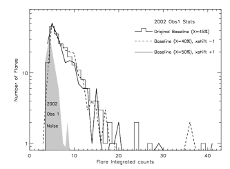
Figure 5.— The distributions of measured flare energies (in XMM-Newton/EPIC counts) for the 2002 Obs. 1 light curve, given three assumed local baseline energies: $X$= 45% (histogram, and the adopted value), $X$=40% (dashed line), which is shifted horizontally by -1 counts in this diagram, and $X$=50% (solid line), shifted by +1 count. The gray area represents “false positive” events measured from the negative count rate variations in this light curve.

As for the importance of random errors masquerading as astrophysical flare events, a key test of the reliability of our measurements was to determine the importance of “false positives” due to photon event fluctuations or possible instrumental or environmental variations. We quantified this test by repeating the measurements for our reference 2002 Obs. 1 light curve yet again and assuming Gaussian distributed errors. This time we used the identical superbin lengths and nearly all other parameters from our first measurements, except that we measured negative fluctuations instead. (The one difference was that we adopted an unbiased value $X$ = 50% for our baseline.) The advantage of this technique was that all possible signal properties (especially the sinuosity of the baseline) are treated exactly the same way as any possible personal equation introduced to the measurements. Unsurprisingly, we found many occurrences of 2 or even 3 consecutive negative fluctuations that were lower than the local mean rate by about 1 rms, but far fewer triggered a false positive that give an integrated count rate algebraically less than -3.7 counts. In all we measured 71 negative detections and tabulated their (negative) count rates and durations. They are exhibited as a gray area in Fig. 5. These should be subtracted against the total measured flare numbers, giving a false positive rate of 17 ${\pm 3}$%. The result shows that the false detections nicely track the lower envelope of so-called weak flares of the measured distribution up to about 5 counts. Essentially all the low envelope positive-fluctuation events in this figure should therefore be regarded as false. The false events fall off quickly toward higher energies, and for 6 counts and above, nearly all the measured events can be regarded as astrophysical.

4.4.3 Flare statistics from XMM-Newton light curves

We also searched for flares in the 2007 time series of HD 110432. However, we limited ourselves to the first 50 ks of the 2007 data to keep the flare statistics errors about the same as for the 2002-2003 datasets. The 2007 data measurements identified 465 flares. Correcting for false positives, this corresponds to an estimated rate of 0.0077 flares s^-1 (386 flares). Our three light curves in 2002–2003 had exposure lengths of 44 to 49 ks, and we found totals of 418, 397, and 335 flares in the three time sequences, respectively. Accounting for a 17% false positives rate, the inferred number of flares detected for observations in 2002–2003, 1150, should actually be 955. Then the mean flare rate for all three datasets is 0.0071$\pm{0.0006}$ flares s^-1, while the means of the three of them are consistent with the overall mean. These are slightly lower than or comparable to the 2007 epoch rate. Including the 2007 data, the false positives-corrected mean rate is 0.0072 flares s^-1

The three XMM-Newton light curves of $\gamma$ Cas we used as controls ($\S$3.2) each had timespans of 15.7-17.5 ks and thus their total length is close to the durations of each of the 2002–2003 HD 110432 light curves. We measured a mean event rate of 0.012 s^-1 for $\gamma$ Cas, corresponding to a total of 541 measured flares. For the superior $\gamma$ Cas data the false positives rate was 4.5%. We therefore subtracted off 24 presumed false positives from the 541 event total, yielding an inferred net of 517 flares. However, the signal-to-noise ratio for these data was a factor of three higher because $\gamma$ Cas’s higher X-ray flux. Therefore, we degraded the SNR of these three light curves with artificial noise in order to match the mean SNR of the HD 110432 sequences. These results were employed to compensate for the differences in X-ray flux and time binning in the datasets for the two stars. The SNR-degraded light curves were again then run through the flarecount program to identify a new total of only 450 flares, giving a frequency of 0.0089 flares s^-1. Again applying the 17% false positives rate determined from HD 110432 to this degraded data, the rate for the $\gamma$ Cas data decreases to 0.0074 flares s^-1. Within the errors this is the same rate as the mean determined for HD 110432. Similarly, we degraded the $\gamma$ Cas RXTE light curve signal for 1996 March (SRC), rebinned to 5 s, and ran flarecount on it to find 201 flares over the same interval. This gives nearly the same mean (uncorrected) frequency of 0.0090 flares s^-1 as the 0.0089 flares s^-1 figure just noted. Thus, when corrected for the difference in signal properties, the flare rates of the various light curves of HD 110432 are about the same.

An important characteristic of the flares is the distribution of their energies, which differs from a power law. These distributions are exhibited logarithmically in Figure 6; flare strength units are XMM-Newton/EPIC counts^-1. Both panels show that the incidence of flare strength (integral over the flare-enhanced count rate) is a monotonically decreasing function. The turnover that exists at low strengths is an artifact of the limited photon statistics. Using the $\gamma$ Cas data again as a control, this turnover (occurring at $\approx$5 counts) is shown by the upper thick dashed lines representing the flare distribution taken from the undegraded (as observed) light curves of $\gamma$ Cas, and as the lower dashed lines from the SNR-degraded light curves. We have computed slopes for the HD 110432 flare distributions shown in Fig. 6 over the abcissa range 6–19 counts. The slope in the log-linear space is -0.065 ${\pm 0.011}$ for the 2007 dataset and -0.011, -0.012, and -0.015 (${\pm 0.002}$ in each case) for the 2002–2003 flares, respectively. These rates are only a little affected by false positive events, most of which occur below the 6 count limit we used to measure the slopes. In any case the relative slopes are almost completely unaffected. These values suggest that at a significance of over 4 sigmas the 2007 flares follow a flatter distribution than the 2002–2003 ones. The 2003 flares have a marginally steeper distribution in turn than the 2002 ones. This suggests that the flare distributions can change slightly on timescales of about a year. RS found a similar range of slopes in flare distributions over a similar timescale.

For HD 110432 the distributions of interflare intervals in Figure 7 are consistent with an exponential distribution for times $\mathrel{\hbox{\hbox to0.0pt{\hbox{\lower 4.0pt\hbox{$\sim$}}\hss}\hbox{$>$}}}$40 s, and thus they appear to occur at random times. The turnover at this time is partially an artifact caused by the limited SNR of the light curves. This is to say, the photon noise sometimes encourages us to measure closely spaced flares as single unresolved ones. (We omitted the strongest flares in our measurements of the logarithmic slopes of the flare strength distributions in Fig. 6 for this reason.) For the distribution of the undegraded light curves of $\gamma$ Cas the turnover is barely discernible. Above 40 s the interflare distribution can be fit to an exponential with an e-folding time of 140${\pm 20}$ s.

Figure 6.— The distribution of measured flare strengths (in XMM-Newton/EPIC counts). All curves in this and following figures are scaled to the number of flares occurring within the 2002 Obs. 1 exposure length (49.4 ks). Thick dashed lines represent two distributions from 2010 light curves of our control, $\gamma$ Cas: the labeled “undegraded” curve denotes the numbers measured from the original data binned to 5 s, while the (unlabeled) SNR-degraded distribution turns down at low energies. Panel a: the HD 110432 distributions for 2002 Obs. 1 and 2003 Obs. 3. Panel b: the HD 110432 distributions for 2007 and 2002 Obs. 2.

The flares in 2007 tend to differ from the 2002-2003 counterparts in their distribution of lifetimes. Taking into account again the noise-generated false events shown in gray, Figure 8 shows that the lifetimes of most flares in 2007 are confined within 10–30 s. Their distribution is almost flat within these limits. In contrast, the 2002 (Obs. 1) and 2003 distributions fall off less rapidly toward short values from a peak at 20–25 s. By comparison, the distribution of lifetimes of the $\gamma$ Cas flares (degraded light curve) most closely resembled the 2007 data of HD 110432. Note also in Fig. 8 that the lifetimes of the HD 110432 flares exhibit an extended, low-amplitude tail out to 80–100 s. In our 2010 $\gamma$ Cas data the longest-live individual flare was 78 s. However, using the full complement of RXTE/PCU detectors, RS found for $\gamma$ Cas that flares in 1996 light curves can occasionally last 150 s. Although noise can cause two closely spaced flares to appear as a stronger unresolved one, the reverse is also true. For example, the strong feature at 26.1 ks in Figure 1 is actually a 4 minute flare aggregate followed immediately by a weaker group lasting 3 minutes. Given these ambiguities, we do not regard the lifetimes and energies of the strongest flares as well defined.

Figure 7.— The distribution of interflare intervals extracted from XMM-Newton light curves of HD 110432 and (undegraded) $\gamma$ Cas. Note the turn over at $\sim$40 s in the HD 110432 distributions.

Figure 8.— The distribution of measured flare lifetimes extracted from XMM-Newton light curves of HD 110342 and (degraded) $\gamma\,$Cas, taken as a control. The gray area represents noise fluctuations in 2002 Obs. 1.

4.4.4 Further comments on strong flares from RXTE data

Our review of flares from HD 110432 was augmented by again degrading the 2007 XMM-Newton light curve to match the SNR of the already low SNR light curve observed by RXTE in 2010 and again measuring flares over an equivalent time interval using the flarecount program. Using the flare selection criteria chosen in $\S$4.4.1, we determined an energy threshold this time of 6 counts. Our results were, first, that the shortest-lived flare events in the degraded time series were 40 s long. Second, we found 61 flares for the 2007 XMM-Newton series and 57 flares for the RXTE series. As in the comparison of the higher quality light curves, these numbers are indistinguishable from one another. Altogether, we conclude that in 2010 HD 110432’s flaring rate was consistent with its value in 2007. As already noted these rates are also consistent with the mean rate for $\gamma$ Cas.

4.4.5 Color dependence of HD 110432’s flares

In comparing the flares statistics assembled from RXTE/PCA and XMM/EPIC data, it is relevant to ask whether the respective instrumental energy responses bias the statistics. We remind the reader that the PCA/PCU’s primary energy sensitivity lies in the range 2–10 keV whereas the EPIC detector responses is broader at both ends. Fully 42% of the 0.6-12 keV photons collected on HD 110432 by the XMM-Newton detectors lies within the soft 0.6-2 keV bandpass. We first compared the XMM-Newton light curve extracted from 2–10 keV (RXTE-like) energies to the 0.6–12 keV energy range and found that basic flare quantities from the two were negligibly different. This implies that there is little or no color bias in the flare statistics between the RXTE and broader band XMM-Newton energy ranges.

An interesting question is whether light curves in the soft and hard X-ray bands always exhibit the same flaring incidence. Figure 9 illustrates this question by showing an example of light curves over several kiloseconds formed from fluxes in the soft band (0.6–2 keV) alone and the full energy range. L07 noted a correspondence of flares in hard and soft energy bands. However, there were occasional departures, suggesting that flares were somewhat more prevalent in a soft band than a hard one. Returning to our flare counting, this time just for 2002 Obs. 1, we found that $\sim$75% of the flares identified in the full energy (0.6–12 keV) were also recovered in the low energy (0.6–2 keV) one. In a smaller fraction of instances (15-20%) the low energy flares were stronger, and occasionally significantly so. Three such examples are highlighted in Fig. 9. Flares could be found only in the soft band even less commonly. A cross correlation of low (0.6–2 keV) and high energy (2–10 keV) light curves disclosed no time lag between them. We can add that color differences in general are more common over timescales of 1 ks or longer. This fact was also noted by the S12 study of a recent XMM-Newton light curve of $\gamma$ Cas.

Figure 9.— A stretch in the 2007 light curve of HD 110432 in two X-ray energy bands (plotted in 100 s bins). Both panels show ubiquitous rapid fluctuations (flares) and slower variations. Flares usually occur at all energies, e.g. within the first ks at times 34.62, 34.88, 35.14, 35.37, & 35.52 ks. The vertical dotted lines are examples of flare complexes that are stronger in the low band than over the full energy range. The converse is at least as common.

5. Other light curve features

In compiling our flare statistics, we found that the distributions of interflare intervals followed apparent exponential distributions down to the shortest interval between detected independent flares. Because we know that we miss the unresolved flares (“aggregates”), we believe this distribution is consistent with a Poisson distribution. This would mean that the flares occur independently of one another. Put another way, there is no indication of clusters or “cascades” of events, such as one finds in true flares on the Sun and late active stars (e.g., Aschwanden 2011). At times the HD 110432 light curves can exhibit as few as two flares per kilosecond, for example, during the extended “drop off” interval discussed next. Within any one of these comparatively flare-free periods, the basal count rate can also decrease for several minutes. This behavior is vaguely reminiscent of the occurrences of much briefer and cyclical lulls that often occur for $\gamma$ Cas (RS, L10). The quasi-periodicity of these events is often 3–3.5 or 7 hours (e.g., RS, L10).

Qualitatively new features appearing as rapid and sustained drop offs are visible in some of the HD 110432 light curves, e.g., the end of RXTE Obs. 2 in Fig. 1 and middle of the 2007 XMM-Newton light curve, which is shown in Fig. 10. These light curves show a step function-like decline (at 35 ks) to a new low count rate level. The rates of decline in these events can occur even over a few minutes, rivaling the decrease and subsequent increase rates in the quasi-periodic lulls of the $\gamma$ Cas light curves. However, they can last as long as 11 hours, as in Fig. 10. A similar, though less dramatic drop in counts can be seen in the RXTE light curve shown in Fig. 1. We have observed no such features in $\gamma$ Cas light curves.

Figure 10.— The 2007 XMM-Newton light curve for the energy range 0.3-12 keV of HD 110432 and binned to 100 seconds. The background count rates are indicated at the bottom. Notice the sharp decrease at time 35 ks referred to in the text. Many positive fluctuations shown are “flares aggregates” discussed in the text. Individual flares generally last for less than 100 seconds and are not resolved in this plot.

6. Discussion and Conclusions

The X-ray light curves of HD 110432 exhibit three types of variability: long cycles of a few months, intermediate variations of a few hours, and rapid flares having lifetimes from 1${\frac{1}{2}}$ minutes down to several seconds. These properties are similar to the ubiquitous X-ray variations in $\gamma$ Cas light curves. The correlation that SRC and SR found between the passages of translucent and hot clouds, according to UV continuum and spectral line time series, and increased X-ray fluxes is key evidence for the X-rays being emitted on or near the surface of the Be star. Since the decommissioning in 1997 of the HST Goddard High Resolution Spectrograph, it has not been possible to confirm this implied causality by simultaneous monitoring stars of HD 110432’s brightness in both X-ray and UV bands.

Even so, our RXTE observations of HD 110432 over six epochs in 2010 (Fig. 2) suggest the existence of a long X-ray cycle similar to those of $\gamma$ Cas. Combining this feature with the optical light cycle (SB) in 2002, we suggest that the long cycles are longer in HD 110432 than in $\gamma$ Cas. We cannot say yet whether the ranges of the cycles in the two stars can overlap.

Likewise, the similar statistical properties for the long cycle oscillations in HD 110342 and $\gamma$ Cas implies a constant ratio of 67–80 for the cycle amplitudes for X-ray and optical variations. If this ratio is indeed universal long “periods” promise to be a boon to the optical discovery of new $\gamma$ Cas analogs.

We have also discussed some unique properties of short-term features in X-ray light curves of HD 110432. One difference in the HD 110432 light is the absence of cyclical, several minute-long lulls found in $\gamma$ Cas light curves. Rather, at least two of our light curves of HD 110432 curves exhibit sudden and sustained decreases in X-ray emission. The more extreme of these events can be described as drop-offs lasting up to several hours. If X-ray flares are the result of bombardments of high energy particles from an external source onto the star, the energy reservoir ultimately powering them seems to become partially depleted for extended intervals. This contrasts with the recurrent lulls in many of the $\gamma$ Cas light curves. This latter description hints of a steady refilling of the reservoir, similar to a relaxation cycle.

In addition, this study and RS have noted differences in the distributions of flare energies and lifetimes at various times. One of these is that the HD 110432 flares in 2007 tend to be slightly more numerous, shorter-lived, and more energetic than those in 2002–2003. Another peculiarity is the apparent log-linear distribution, which seems to be different from the power law relation for solar flares. It is not yet clear how these differences can be understood within even a general paradigm. In any case we would want to extend the flare count distribution to a larger range before being satisfied with this conclusion. At the risk of speculation, we can point out that in the RS picture, according to which the mean energies of flares is proportional to the input mean beam energy, $<$E$>$, the latter energy seem to be slightly higher in 2007. If so the beams would penetrate to greater atmospheric densities. This would account for the more energetic and the preponderance of shorter-lived flares observed at that time. These differences would require more a complicated explanation in the blob accretion picture.

We have reported that most flares do not exhibit color changes in HD 110432, as has also been reported for $\gamma$ Cas (RS). However, L07 already pointed out the sometime occurrence of soft-energy flares. In this study we have found examples of flares that occur at hard energies but are weak or absent in the soft band. In fewer cases we also discovered flares more prominent in the soft band. This also gives us the impression that the energy excitation mechanism responsible for flares sometimes operates over a range of energies although the high end usually dominates. In our picture X-ray flares are created by bombardments from without and are only the manifestation of this high energy input. RS have discussed how such color changes (including the sometimes observed inequality $T_{flare}$ $<$ $T_{basal}$) can be produced by introducing a small range in a beam energy distribution.

To sum up, the X-ray variability of HD 110432 over a variety of timescales is similar to that of $\gamma$ Cas. A comparison of their flare incidences at different times showed that they can vary by small amounts, but the degree and timescale of changes from a mean rate are not yet clear. Likewise, while we are not yet able to corroborate that the optical and X-ray long cycles are associated with each other for this star, a comparison of their basic properties (perhaps including a common ratio of the X-ray and optical variations, L${}_{x_{max}}$/L${}_{x_{min}}$)/$\triangle V$) for both HD 110432 and $\gamma$ Cas suggests that the long cycles are common to $\gamma$ Cas stars at large. The cycle lengths likewise vary over time and their mean lengths may even differ from star to star. It will be of interest to see how these lengths are related to general disk characteristics inferred from optical observations.