Disentangling Confused Stars at the Galactic Center with Long Baseline Infrared Interferometry

Abstract

We present simulations of Keck Interferometer ASTRA and VLTI GRAVITY observations of mock star fields in orbit within $\sim 50$ milliarcseconds of Sgr A*. Dual-field phase referencing techniques, as implemented on ASTRA and planned for GRAVITY, will provide the sensitivity to observe Sgr A* with long-baseline infrared interferometers. Our results show an improvement in the confusion noise limit over current astrometric surveys, opening a window to study stellar sources in the region. Since the Keck Interferometer has only a single baseline, the improvement in the confusion limit depends on source position angles. The GRAVITY instrument will yield a more compact and symmetric PSF, providing an improvement in confusion noise which will not depend as strongly on position angle. Our Keck results show the ability to characterize the star field as containing zero, few, or many bright stellar sources. We are also able to detect and track a source down to $m_{K}\sim 18$ through the least confused regions of our field of view at a precision of $\sim 200~{}\mu$as along the baseline direction. This level of precision improves with source brightness. Our GRAVITY results show the potential to detect and track multiple sources in the field. GRAVITY will perform $\sim 10~{}\mu$as astrometry on a $m_{K}=16.3$ source and $\sim 200~{}\mu$as astrometry on a $m_{K}=18.8$ source in six hours of monitoring a crowded field. Monitoring the orbits of several stars will provide the ability to distinguish between multiple post-Newtonian orbital effects, including those due to an extended mass distribution around Sgr A* and to low-order General Relativistic effects. ASTRA and GRAVITY both have the potential to detect and monitor sources very close to Sgr A*. Early characterizations of the field by ASTRA including the possibility of a precise source detection, could provide valuable information for future GRAVITY implementation and observation.

1 Introduction

Over the last 20 years, high resolution infrared imaging techniques have provided precise astrometric measurements of stellar sources at the Galactic Center. Focused astrometric monitoring campaigns have revealed a population of mostly young early-type stars (the S-cluster) in orbit about the location of the radio and infrared source dubbed Sagittarius A* (Sgr A*). In fact, Ghez et al. (2008) and Gillessen et al. (2009) both analyze their own distinct data sets to deduce a mass of $4.5\pm 0.4\times 10^{6}\mathrm{M}_{\odot}$ located coincident with Sgr A*. This mass must all be within the periapsis of the star S16/S0-16, which is only  40 AU. The implied mass density provides compelling proof that Sgr A* is the luminous manifestation of an accreting black hole. In addition to providing a measurement of the mass of Sgr A*, the orbits of the stars also provide a direct measurement of the distance to the black hole, $8.36\pm 0.44$ kpc (Ghez et al., 2008).

If Sgr A* actually resides at the dynamic center of the Milky Way, then measuring its distance also represents a measurement of the solar distance from the Galactic Center ($R_{0}$). Monitoring stellar orbits about Sgr A* also provide a measurement of the sun’s peculiar motion in the direction of the Galactic Center ($\Theta_{0}$). As discussed by Olling & Merrifield (2000), $R_{0}$ and $\Theta_{0}$ are ubiquitous parameters in the description of the structure and dynamics of the Milky Way (see also Reid et al., 2009). Uncertainty in the values of $R_{0}$ and $\Theta_{0}$ are the largest sources of error in the determination of the ratio of the galactic halo’s long and short axes ($q$, Olling & Merrifield, 2000). The parameter $q$ is sensitive to different galaxy formation scenarios and dark matter candidates, and if $R_{0}$ and $\Theta_{0}$ were known at the $1\%$ level, the constraints on $q$ would help to differentiate theories of galaxy formation and dark matter (Olling & Merrifield, 2000). In addition, a very precise knowledge of $R_{0}$ could affect our calibration of the lowest rungs of the cosmic distance ladder by improving our distance measurements to galactic sources such as Cepheids and RR Lyrae variables(Ghez et al., 2008).

The existence of the S-cluster is intriguing because it is rich with young stars and because forming these stars in situ represents a theoretical problem given the strong tidal forces in the region. The alternative of formation at larger radii and subsequent migration is strongly constrained by the deduced young age of the stars. However, because the S-stars are known to be younger than the relaxation time in the environment (a B star’s main-sequence lifetime is $\sim 10^{7}$ years compared to the relaxation time of $\sim 2\times 10^{8}$ years; Weinberg et al., 2005) their orbits should encode some information about the kinematics of the cluster at the time it formed. Thus, perhaps as a bonus, astrometric monitoring of the stars in our Galaxy’s nuclear cluster has the potential to inform the community not only on matters of General Relativity and galaxy formation, but also on star formation in extreme environments.

The deduced mass and distance of Sgr A* make it the largest black hole on the sky, in terms of angular diameter, and an excellent candidate for study. Improving astrometric measurements and discovering stars on even shorter period orbits will improve our understanding of the gravitational potential which binds the stars, possibly exposing a dark matter cusp at the center of our galaxy, and should inform our understanding of gravity on scales not yet explored by precise experiments. For example, Weinberg et al. (2005) modeled a distribution of stars on very short period orbits about Sgr A* and showed that post-Newtonian effects on the orbital paths could be detected with the astrometric precision and sensitivity of a future thirty-meter telescope. Existing and upcoming near-IR interferometers can provide even better resolution, and enable some of the same science. In their treatment Weinberg et al. (2005) assumed Gaussian point spread functions, which tend to zero in the wings faster than the more realistic Airy pattern which distributes light in rings away from the central core. These rings present a contrast barrier in conventional imaging. Likewise, the even more complicated point spread functions (PSFs) provided by interferometers result in contrast and detection limits and can bias astrometric measurements.

Fritz et al. (2010) showed that halo noise and source confusion are the factors limiting astrometric accuracy. These effects, which are both related to the angular resolution of the telescope and the luminosity function of the sources in the region (i.e. the dynamic range), present a fundamental astrometric hurdle which cannot be overcome with even the largest single aperture telescopes of today (Ghez et al., 2008; Gillessen et al., 2009). In fact, simulations by Ghez et al. (2008) and Gillessen et al. (2009) showed that astrometric errors could be as large as 3 milliarcseconds due to confusion with undetected sources. This level of astrometric uncertainty, present close to Sgr A* where stars experience the deepest part of the potential, has precluded the detection of any post-Newtonian effects on stellar orbits to this point and has limited the precision with which the distance to the Galactic Center can be measured.

The limiting magnitude and astrometric precision of Galactic Center observations has improved as early speckle observations (e.g. Eckart et al., 1992) were supplemented by adaptive optics (AO) and laser guide star AO (e.g. Ghez et al., 2005). The current state of the art is a limiting magnitude of $\sim$19 at K and an astrometric precision of $\sim 100\mu$as. However, these limits are only achieved far from the crowded central region immediately surrounding Sgr A*. In this paper we investigate whether, with the increased resolution of infrared interferometers and the concomitant reduction in confusion, we can detect heretofore undetected or unnoticed stars on orbits with very short periods within 50 mas of Sgr A*. We also explore the astrometric precision with which such sources could be monitored with an IR interferometer. According to Ghez (2010) a factor of $\sim 3$ more stars with periods less than 20 yrs are expected to be orbiting Sgr A*. These stars, if they can be detected and monitored, will provide a detailed description of the central potential (a minimum of three short-period orbits are required for a complete characterization; Rubilar & Eckart, 2001). Additionally, such stars will provide the best targets for observing General Relativistic effects since they are deepest in the potential well of Sgr A*.

Although the higher resolution provided by interferometry is beneficial for increasing the detectability of sources in the crowded region and for increasing the astrometric precision attainable, there are many potential complicating factors which do not apply to conventional full aperture imaging. For example, in full aperture imaging, collecting area increases as the square of the resolution. In interferometers, however, the collecting area is independent of the effective spatial resolution. This means that although the confusion limit is somewhat alleviated by the higher angular resolution available, photon noise quickly becomes a problem in the detection of faint sources. This fact is further exacerbated by the low typical throughput of interferometers (e.g., $\sim 2\%$ for the Keck Interferometer). Additionally, the sparse nature of an interferometer’s collecting area results in an incomplete sampling of the Fourier components of the source distribution on the sky. This causes an incomplete knowledge of the sky-plane light distribution resulting in PSFs with large sidelobes. Finally, Michelson interferometers like the Keck Interferometer and the VLT Interferometer (VLTI) have small fields of view, $\sim 50$ mas, which typically only include a single object; clearly this presents difficulty for astrometry. We attempt to understand the scale of these effects by simulating data and inferring results.

The outline of the paper is as follows. In Section 2 we discuss the construction of mock star fields within 50 mas of the Galactic Center. In Section 3 we discuss our observation simulator and all included sources of noise and uncertainty. Section 4 covers our algorithm for making relative astrometric measurements by fitting to the visibility curves. Section 5 includes a presentation of our results. Section 6 provides a discussion of the potential advances and difficulties. Although we try to keep the discussion general, we focus on ASTRA at the Keck Interferometer as we are most familiar with that instrument and it is currently capable of making these observations. We also provide a discussion of VLTI GRAVITY (Eisenhauer et al., 2008) simulations.

2 Simulating a Star Field within 50 Milliarcseconds of Sgr A*

Interferometric observations of the Galactic Center will be conducted through the K band. We construct mock star fields in orbit about the black hole at the Galactic Center using as much information about the number of sources and the distribution of K band magnitudes as is available. Previous observations, while limited by confusion noise, have provided a wealth of information regarding the stellar population and K-band luminosity function (KLF) of the central cluster. Genzel et al. (2003) showed that the KLF of the inner 1.5” around Sgr A* is well fit by a power law with a slope of $\beta=\frac{d\mathrm{log}N}{dK}=0.21\pm 0.03$. Weinberg et al. (2005), for example, used this luminosity function normalized to the photometry of Schödel et al. (2002) of the stars within 0.8” of Sgr A* to extrapolate the population of stars even closer to the Galactic Center.

Additionally, some clues about the content of the confused region can be gleaned from observations of well-monitored stars— stars on orbits which spend most of their time outside of the confused region— when they pass through the confused region during their orbital periapsis. For example, when the star S0-2 passed through periapsis in 2002 its centroid was offset from its fitted orbital path. This offset strongly suggests a confusion event with an undetected source (or multiple undetected objects). By measuring the offset and the ellipticity, or lack thereof, of the S0-2 PSF during 2002, some constraints on the unseen source(s) can be derived (e.g. Gillessen et al., 2009).

Further, both Do et al. (2009) and Dodds-Eden et al. (2011) provide analyses of Sgr A* light curves and show a median magnitude in K-band of $\gtrsim$ 16 and a minimum magnitude of $\gtrsim$ 17. While absolute photometry in the region is complicated by confusion noise, we use the analyses of Sgr A* lightcurves to normalize two separate star fields for use in our study. In our first star field, Field1, we set the flux from Sgr A* equal to its median observed value, the flux from the brightest star in the field we set to be consistent with the minimum observed flux from the region as reported in Do et al. (2009) and Dodds-Eden et al. (2011), and we include three fainter stellar sources consistent with an extrapolation of the KLF reported in Genzel et al. (2003) (see their Table 2). To be cautious, we also model a second star field in which we have decreased the flux of each source by one magnitude. This fainter star field we call Field2. We believe that these two fields should encompass a fair representation of the true source distribution very close to Sgr A*.

While we took care that our star fields are consistent with available observations, the true source content within 50 milliarcseconds is unknown. The potential to further constrain the stellar content within the region is one the scientific motivations for observing the Galactic Center with long-baseline infrared interferometers.

We assigned spectral slopes to our sources to be consistent with the observed slopes of sources near the Galactic Center, namely $\alpha=2.3\pm 0.1$ for $F_{\lambda}\propto\lambda^{\alpha}$. The spectral slope of Sgr A* was taken to be $\alpha=4.5$ (Tuan Do, private communication; see also Do et al. (2009) and Paumard et al. (2006)).

While we modeled Sgr A* as stationary, the stellar sources were assigned random Keplerian orbits with semi-major axes in the range of 0.1-400 AU. We chose this range of semi-major axes to coincide with the confused region around Sgr A*. Any source with a larger semi-major axis should leave this region, and would likely have been detected in previous AO observations. Table 1 shows the modeled parameters for our star fields.

Table 1: Model star field parameters for our simulated fields.

Source	Field1 [$m_{K}$]	Field2 [$m_{K}$]	spectral slope	Period [yrs]	e	$\tau[\mathrm{yrs}]$	$\Omega[\mathrm{rad}]$	$i[\mathrm{rad}]$	$\omega[\mathrm{rad}]$
Sgr A*	16.3	17.3	4.5	–	–	–	–	–	–
Star 1	16.9	17.9	2.28	1.75	0.44	0.93	5.32	0.68	4.19
Star 2	18.8	19.8	2.34	2.65	0.12	0.60	2.61	1.36	4.89
Star 3	20.3	21.3	2.31	0.24	0.90	0.20	4.64	-0.61	2.95
Star 4	20.6	21.6	2.14	2.31	0.74	1.53	1.16	1.07	0.91

Note. — We assumed random Keplerian orbits for our modeled sources. $\tau$ is the time of periapsis passage in years since January 1, $\Omega$ is the longitude of the ascending node, $i$ is the inclination, and $\omega$ is the argument of periapsis.

3 Synthesizing Visibility Data

3.1 Basic Concepts

Interferometers combine light from a source collected at more than one aperture, forming an interference pattern. This interference pattern encodes high spatial frequency information of the light distribution under observation. The maximum spatial frequency which can be detected by an interferometer can be expressed succinctly as $\frac{B_{\mathrm{proj}}}{\lambda}$, where $\lambda$ is the wavelength of the observation and $B_{\mathrm{proj}}$ is defined as the projection of the vector connecting the two apertures onto the plane of the sky in the direction of observation. The interference pattern of light created by a monochromatic source can be described as

$$P(\delta)=P_{1}+P_{2}+2\sqrt{P_{1}P_{2}}\mathrm{Re}\{Ve^{ik\delta}\})$$ (1)

or

$$P(\delta)=P_{1}+P_{2}+2\sqrt{P_{1}P_{2}}|V|\cos(k(\mathrm{arg}(V)+\delta)))$$ (2)

where $P_{1}$ and $P_{2}$ are the incident power from each aperture, $k$ is the wave number, $\delta$ is the relative path-length delay between the two apertures, and $V$ is the complex visibility (see e.g. Lawson, 2000).

The polychromatic case is slightly more complicated, and a brief discussion of the effects of a finite bandwidth on interference fringes will help elucidate some of the challenges of practical interferometry. In general, astronomical sources radiate polychromatic light such that each wavelength of light is mutually incoherent with every other wavelength. The result of this mutual incoherence is that polychromatic fringes are a sum of fringes produced by each individual wavelength of light. Since a fixed $\delta$ will result in a different phase offset between the two apertures for each wavelength of light (i.e. $\phi=k\delta$), it is impossible to keep fringes arising from different wavelengths of light in phase everywhere. Polychromatic fringes are only present in the neighborhood of zero delay and are attenuated as $\delta$ increases. In fact, the fringes are attenuated by an envelope function which takes the shape of the Fourier transform of the spectral bandpass. For the case of a top-hat bandpass centered at $\lambda_{0}$ and with a width of $\Delta\lambda$, the envelope takes the shape of a sinc function, and fringes are detected inside the coherence length

$$\Lambda\equiv\frac{\lambda_{0}^{2}}{\Delta\lambda}.$$ (3)

For a typical case of five spectral channels in the K band, $\Lambda\sim 25\lambda$ (see Table 2). This imposes a strict requirement on the implementation of interferometric measurements. In general, the path lengths of light incident on different telescopes must be similar to within $\Lambda$ before being combined if fringes are to be observed at all. Even more strictly, $\delta$ must be less than $\frac{\lambda}{B_{\mathrm{proj}}}$ if the central unattenuated “white-light” fringe is to be observed. This necessitates delay lines to precisely correct for the optical path length difference between the two apertures. Further, the existence of a coherence envelope also imposes a restriction on our field of view. For a Michelson Interferometer the field of view can be calculated according to

$$\mathrm{FOV}=\frac{\Lambda}{B_{\mathrm{proj}}}.$$ (4)

Table 2 lists $\Lambda$ and the corresponding field of view for each of the modeled spectral channels using the Keck Interferometer.

Table 2: Coherence Length

$\lambda_{0}$ [microns]	$\Delta\lambda$ [microns]	$\Lambda$ [microns]	Field of View [mas]
2.0	0.087	45.97	141.99
2.09	0.091	48.00	148.25
2.18	0.095	50.02	154.49
2.28	0.099	52.50	162.15
2.38	0.104	54.46	168.21

Note. — The central wavelength and width of the spectral channels for our observations. Also shown are the corresponding coherence length and implied field of view. As we will see in Section 3.2, the true limiting factor for our field of view will be the fiber response function which is modeled to have a full width at half maximum of 55 mas.

Atmospheric turbulence induces a differential delay between the two telescopes, $\delta_{\mathrm{atmosphere}}$, which is variable on timescales of $t_{\mathrm{turb}}\sim\frac{D}{v_{\mathrm{wind}}}$, with $D$ the diameter of each aperture and $v_{wind}$ the wind velocity. If an exposure time of longer than $\sim t_{\mathrm{turb}}$ is required, the delay lines at the interferometer, which are responsible for keeping $\delta\approx 0$, cannot only compensate for sidereal motion or else fringes will be smeared; atmospheric delay must be detected and corrected for dynamically.

Because the Galactic Center is faint, a dual field system is required to incorporate a bright reference star for fringe tracking. In dual field phase referencing (DFPR) a field separator is used to create two beam trains, one with a bright reference source and one with a fainter science target. Similar to natural guide star adaptive optics, light from the bright reference star is used to detect and measure the differential atmospheric delay. These measurements are enabled by the high flux of the reference source, which allows for short exposures of less than $t_{\mathrm{turb}}$.

Precise metrology is required for the application of a dual field system. Delay line commands need to be precise on the order of a fraction of the fringe spacing, which is typically $\sim 0.03$ microns for our scenarios observing in the K band. Also important, a precise baseline measurement is needed to perform the conversion from delay offset of the reference fringes to a delay line command in the science beam. The situation is complicated since there are two beamtrains, each with distinct path lengths which must be measured continuously to monitor fluctuations due to thermal drifts and other effects.

3.2 Sources of Uncertainty for Phase Referenced Interferometric Imaging

Visibility measurements entail measuring the amplitude and phase of interference fringes using a light detector. Any corruption of fringe amplitude, fringe phase, or flux levels on the detector must be taken into account. Below we describe all such influences considered.

A fringe-tracker measures the phase of the fringes in the reference beam and sends corrections to delay lines. The finite servo bandwidth in the fringe-tracker will cause the observed fringes to be smeared, and lowering the observed amplitude by a factor which we take to be:

$$C_{\mathrm{servo}}=0.75,$$ (5)

consistent with the performance of phase referencing at the Palomar Testbed Interferometer (Lane & Colavita, 2003).

In DFPR the reference source and the science target are observed through different portions of the atmosphere, each with slightly different piston aberrations (anisopistonism, Esposito et al., 2000; Colavita, 2009). Thus the assumption that light from the science target can be held in phase by monitoring the phase of the brighter reference source will introduce an error. This error will smear the fringes and reduce the modulus of the visibility. The size of this effect is discussed in Esposito et al. (2000) and Colavita (2009) and is given as

$$C_{\mathrm{aniso}}=\mathrm{exp}(-0.44(\frac{\theta}{\theta_{p}})^{2})$$ (6)

where $\theta_{p}$ is the isopistonic angle given by Esposito et al. (2000), and $\theta$ is the angle to the reference star.

After the cophased beams are combined, the light passes through single-mode fiber optic cables and then to the camera. Fibers respond best to on-axis sources and transmit only a fraction of the light from off-axis sources. This reduces the observed flux of each source by a factor of $F(\alpha,\beta)$, where $F$ is the fiber function defined below and $\alpha$ and $\beta$ are the position of each source relative to the phase center. We model the fiber response function as achromatic with a Gaussian function having a full width at half maximum of 55 milliarcseconds:

$$F(\alpha,\beta)=\exp(-4\log(2)\frac{\alpha^{2}+\beta^{2}}{(55\mathrm{mas})^{2}}).$$ (7)

Pointing errors also affect our astrometric precision. In interferometry, pointing errors are manifest as phase errors in the complex visibilities. We account for phase errors arising from a handful of instrumental effects primarily related to measuring and monitoring the baseline and internal paths. We label the combined contribution of these effects $\sigma_{\mathrm{metrology}}$. Another phase error that affects our ability to point arises due to the different paths light from separate sources take through the atmosphere. As discussed by Shao & Colavita (1992), the uncertainty in the observed phase of interferometric fringes can be written as

$$\sigma_{\mathrm{atmosphere}}\approx 300B^{\frac{-2}{3}}\theta t^{\frac{-1}{2}}~{}\mathrm{arcseconds},$$ (8)

where $B$ is the projected baseline in meters, $\theta$ is the angular separation between the science target and a reference source in radians, and $t$ is the integration time in seconds. This relationship is calibrated using models of the atmosphere above Mauna Kea. We combine the two sources of phase error to produce a total pointing error:

$$\sigma_{\mathrm{point}}^{2}=\sigma_{\mathrm{metrology}}^{2}+\sigma_{\mathrm{atmosphere}}^{2}.$$ (9)

We measure the visibility amplitude and phase using the four-bin ABCD algorithm (Colavita, 1999). In the ABCD algorithm the average intensity in each quarter fringe (A,B,C,and D) is measured and used to deduce the complex visibility. The real and imaginary parts of the visibility can be calculated according to:

$$\mathrm{Re}\{V\}=A-C,$$ (10)

and

$$\mathrm{Imag}\{V\}=B-D.$$ (11)

Since each measurement A through D is a flux measurement, each is susceptible to normal photometric uncertainties including Strehl fluctuations, photon noise, and readout noise. We assume $\sigma_{\mathrm{Strehl}}=10\%$ injection fluctuations, which account for Strehl variations and for the variable coupling of speckles from bright sources beyond our field of view into the fiber (speckle coupling). We assume an average Strehl in the K band of 35%. While this value of the Strehl is consistent with typical values in previous laser guide star AO observations (e.g Ghez et al., 2005), it may represent an optimistic estimate for performance with ASTRA. This is because reported Strehl ratios in the literature are likely to be biased high by frame selection. In our simulations, a reduced Strehl ratio will result in a lower level of flux in the fringes. In our results section below, we demonstrate how our performance scales with flux by modeling two starfields which are identical except that in one all source fluxes have been scaled by one magnitude.

Bright stars on the periphery of our field of view also have the potential to affect our simulated visibilities. This is because, as shown in Table 2, the interferometric coherence envelope extends out to a radius $\sim 70$ mas and because the fiber will have at least some response there. We assume that such bright sources at large radii have already been detected with laser guide star AO observations and that their effect on our visibilities could be modeled out accordingly.

We report our modeled background flux levels in each spectral channel in Table 3. They are based on observed background performance using the Keck Interferometer fringe tracker (e.g. Woillez et al., 2012). The read noise, $\sigma_{\mathrm{rdnz}}$, is taken to be 10 counts, consistent with the performance of the Hawaii arrays at Keck. Thus we take the uncertainty in each read in each spectral channel to be

$$\sigma_{\mathrm{detect}}^{2}=t_{\mathrm{int}}(\sum_{j}(F(\alpha_{j},\beta_{j})(0.35+\eta_{1}+0.35+\eta_{2})(P_{j}))+P_{\mathrm{bg}}+\sigma_{\mathrm{rdnz}}^{2}$$ (12)

where $j$ indexes each source in the field, $\alpha_{j}$ and $\beta_{j}$ are he position of each source on the fiber, $P_{j}$ is the flux on each aperture emanating from each source, and $P_{\mathrm{bg}}$ is the background flux. The exposure time $t_{\mathrm{int}}$ is the time spent on each read, and $\eta_{1}$ and $\eta_{2}$ are sampled values of the injection fluctuations drawn from a Gaussian distribution of standard deviation $\sigma_{\mathrm{Strehl}}$.

Our modeled observational setup uses 60 five-second subreads per 300-second block. Each subread includes one second of integration on each fringe quadrature and one second on a bias frame. A summary of our simulator parameters can be found in Table 3.

3.3 Producing Mock Fringes

In the previous section, we described the magnitude of several corrupting influences including several random noise sources. Actual values for each of these random sources of noise must be realized before we can produce our simulated fringes. We assign to the variable $\phi_{\mathrm{err}}$ a sampled value of the random pointing error drawn from a Gaussian distribution of width $\sigma_{\mathrm{point}}$. For each aperture we draw a value for the random injection fluctuation from a Gaussian of width $\sigma_{\mathrm{Strehl}}$; we assign these values to the variable $\eta_{i}$, where $i$ indexes the aperture. Finally, we generate a value, $n_{\mathrm{detect}}$, for the detection noise by drawing from a Gaussian distribution of width $\sigma_{\mathrm{detect}}$.

Next, we combine the random noise sources with calculated values for $C_{\mathrm{aniso}}$, the fiber attenuation function, and the visibility of each individual point source to model and measure the fringes as follows

$$\hat{E}(\delta)=t_{\mathrm{int}}((0.5+\eta_{1})P+(0.5+\eta_{2})P+2\sqrt{(0.5+\eta_{1})(0.5+\eta_{2})P^{2}}|\hat{V}|\cos(k(\mathrm{arg}(\hat{V})+\delta)))$$ (13)

where the amplitude and phase of the fringes are specified by the complex visibility given by

$$\hat{V}=\frac{\sum_{j}F(\alpha_{j},\beta_{j})P_{j}C_{\mathrm{servo}}C_{\mathrm{aniso}}V_{\mathrm{point}}(\alpha_{j},\beta_{j},u,v)e^{2\pi i\phi_{\mathrm{err}}}}{\sum_{j}F(\alpha_{j},\beta_{j})P_{j}}.$$ (14)

Here $V_{\mathrm{point}}(\alpha,\beta,u,v)$ is the complex visibility of a point source (see e.g. Lawson, 2000), $t_{\mathrm{int}}$ is the exposure time (1 second in our model). The quadratures are then determined using

$$\hat{A}=\frac{\int_{0}^{\frac{\pi}{2}}\hat{E}_{A}(\delta)\,\mathrm{d}\delta}{\frac{\pi}{2}}+n_{\mathrm{detectA}}$$ (15)

$$\hat{B}=\frac{\int_{\frac{\pi}{2}}^{\pi}\hat{E}_{B}(\delta)\,\mathrm{d}\delta}{\frac{\pi}{2}}+n_{\mathrm{detectB}}$$ (16)

$$\hat{C}=\frac{\int_{\pi}^{\frac{3\pi}{2}}\hat{E}_{C}(\delta)\,\mathrm{d}\delta}{\frac{\pi}{2}}+n_{\mathrm{detectC}}$$ (17)

$$\hat{D}=\frac{\int_{\frac{3\pi}{2}}^{2\pi}\hat{E}_{D}(\delta)\,\mathrm{d}\delta}{\frac{\pi}{2}}+n_{\mathrm{detectD}}$$ (18)

For each hour angle and wavelength observed, the real and imaginary parts of the visibility are then reported as $\hat{A}-\hat{C}$ and $\hat{B}-\hat{D}$ respectively. It is important to note that a new realization of $\hat{E}$ is made for each quadrature, exposing each quadrature to independent injection fluctuations. This inter-ABCD fluctuation affects both the deduced amplitude and phase of the complex visibility, and is often the dominant noise source.

Table 3: Parameters

Parameter	Keck	VLTI	Shared
Number of baselines	1	6	—
Time on source each observing night	3 hours	6 hours	—
Blocktime	—	—	300 seconds
Transmission	1.7%	0.9%	—
Fiber full width half maximum	—	—	55 milliarcseconds
Strehl	—	—	35%
Injection Fluctuations ($\eta$)	—	—	10%
Background flux rate in each channel	—	—	60, 167, 430, 1112, and 2677 photons/second
$\sigma_{\mathrm{readnoise}}$	—	—	10 counts
Decoherence Due to the servo ($C_{\mathrm{servo}}$)	—	—	0.75
Isopistonic angle ($\theta_{\mathrm{p}}$)	13.5 arcseconds	16.1 arcseconds	—
Distance to fringe tracking star ($\theta$)	7 arcseconds	1.2 arcseconds	—
Decoherence due to anisopistonism ($C_{\mathrm{aniso}}$)	0.90	0.998	—
$\sigma_{\mathrm{atmosphere}}$	$32\--42\mu\mathrm{as}$	$4\--7\mu\mathrm{as}$	—
$\sigma_{\mathrm{metrology}}$	$20~{}\mu\mathrm{as}$	$14.5~{}\mu\mathrm{as}$	—

8 and is a function of baseline. For the VLTI we report the mean value for the six baselines.

Note. — Our error values are reported for 300 second blocks. Where applicable they will average down. For example, in three hours, $\sigma_{\mathrm{atmosphere}}$ for Keck Interferometer is $\sim 7.2\mu$as. For the VLTI in six hours, $\sigma_{\mathrm{atmosphere}}\sim 1\mu$as

3.4 Observing Routine, UV-coverage, and PSFs

We simulate observations for two instruments: ASTRA at the Keck Interferometer and GRAVITY at the VLTI. For the Keck Interferometer/ASTRA our adopted observing routine assumes 10 visits to Sgr A* per night at even intervals between the hour angles of -1.5 and 1.5. This is the maximum hour angle range for which Sgr A* is above $\sim 50^{\circ}$ Zenith Angle. For the VLTI, we modeled 20 visits to Sgr A* per night between the hour angles of -3 and 3. This reflects the higher transit of Sgr A* at the location of Cerro Paranal and assumes a similar observational cadence is attainable at both the Keck Interferometer and VLTI. Individual observations are assumed to last 10 minutes with 5 minutes of on-source integration. We model fringes in 5 spectral channels dispersed across the K-band (see Table 2). Ten observations in five spectral channels per night provide 50 visibilities from the Keck interferometer. 20 observations in five spectral channels over 6 baselines provide 600 visibilities per night at the VLTI.

The resulting uv-coverage and PSF for the Keck Interferometer is shown in Figure 1. The PSF is narrow, $\sim 5$ mas at half maximum, along the direction of the interferometer baseline, but extended in the perpendicular direction. Because of the distinct shape of the Keck Interferometer PSF, we will measure astrometry much more precisely along the baseline than in the orthogonal direction. The extended wings or sidelobes of the PSF will have the tendency to overlap when the separation between sources has only a very small component along the baseline direction. Such overlapping sidelobes bias astrometric measurements (see below). However, within $\sim 50$ mas of the Galactic Center, where stars are expected to be orbiting with periods $\sim 1$ year and $~{}1-2$ bright sources are expected in the field, multi-epoch observations with the Keck Interferometer stand a good chance of observing the sources with significant separation along the baseline angle (see Section 5.1 below).

The extended wings of the Keck Interferometer PSF shown in Figure 1 will result in a restricted contrast limit. This is because flux from a bright source is distributed throughout the field in the wings of the PSF. To be detectable in the vicinity of a bright source, a faint source must be brighter than the noise in the wings.

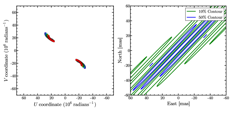
Figure 1: The uv-coverage (left), and the 10% and 50% contours of the resulting PSF (right) produced by our adopted observing routine at the Keck Interferometer.

Our adopted VLTI observing routine provides the uv-coverage shown in the left panel of Figure 2. The increased uv-coverage provided should have an easier time distinguishing sources in a crowded field.

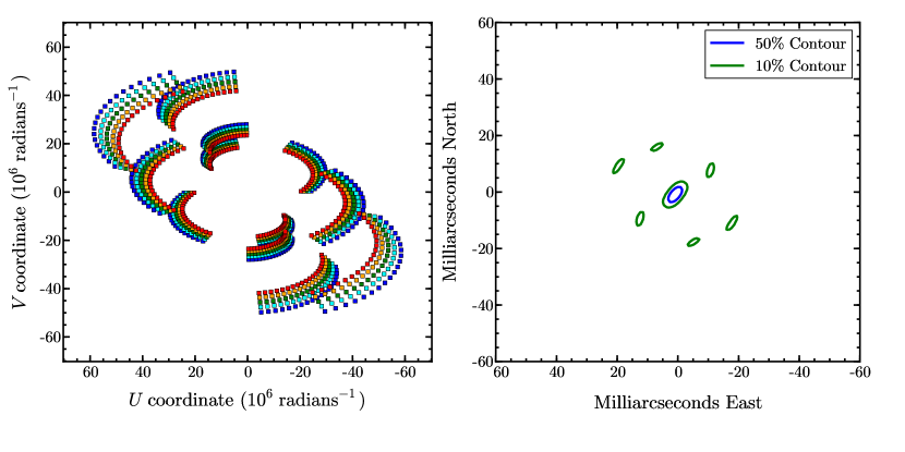
Figure 2: Left: The uv coverage provided by the VLTI in six hours of observing the Galactic Center. Right: The 10% and the 50% contours of the synthesized beam.

4 Fitting Stellar Positions to Visibility Data

There are four free parameters for each source in the field: position ($x$,$y$), flux, and spectral slope. For real data, the number of sources in the field will not be known a priori. In order to efficiently search the large parameter space for a best fit to the synthesized data, we implement a hybrid grid fit and Levenberg Marquardt (LM) minimization algorithm to minimize the $\chi^{2}$ function of the parameters given the synthesized data.

The interferometric visibility produced by a distribution of point sources is expected to be undulating versus baseline (Figure 4) and thus the $\chi^{2}$ surface in the $x_{k},y_{k}$ plane is expected to be similarly undulating (see Figure 3 for a slice through the range of the $\chi^{2}$ function in the $x_{k},y_{k}$ plane). Since the Levenberg Marquardt algorithm is a gradient fitting algorithm which always proceeds “downhill” from an initial starting point— which must be supplied by the user— the undulating nature of the $\chi^{2}$ surface can present a problem because the LM algorithm will converge on a local minimum if the initial parameters are not in the neighborhood of the global minimum. We have therefore adopted a grid-based approach to ensure that starting values supplied to the LM fitter sample the $\chi^{2}$ surface well enough to ensure at least one seed begins in the neighborhood of the global minimum. Since local minima on the $\chi^{2}$ surface mirror local maxima in the PSF, local minima will be separated by about the interferometer fringe spacing. Thus, we used a grid spacing of $\frac{\lambda_{\mathrm{min}}}{B_{\mathrm{max}}}$, where $\lambda_{\mathrm{min}}$ is the shortest wavelength observed and $B_{\mathrm{max}}$ is the longest projected baseline used. Figure 3 shows our grid of seed parameters.

To begin, we start with a model consisting of two point sources. For the fit, we seed an LM fitter with a grid of starting locations (shown in Figure 3) and a guess of the flux and spectral slope of each source. We then use the best-fit values of this fit together with an additional grid of starting locations to seed a 3-source model fit. This process can then be repeated to fit for any number of sources. We do not know how many sources will be present in real data, so we are guided by the significance of the fits and the deduced flux of the fitted sources. Highly significant fits and sources with large fitted fluxes are taken to be real, and less significant fits are disregarded.

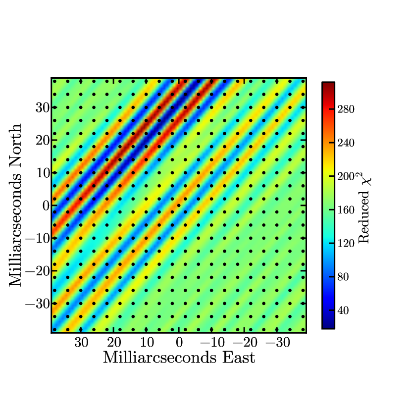
Figure 3: A slice through the reduced $\chi^{2}$ surface for a fit of a two-source model to Keck Interferometer data. The undulations present a hurdle to the naive application of a gradient fitting algorithm since there is the potential to converge on a local minimum. Over plotted on the $\chi^{2}$ surface is the grid of seed positions provided to the gradient fitting algorithm. The grid spacing ensures that the global minimum is sampled.

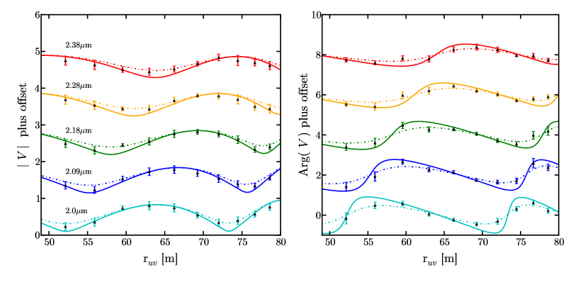
Figure 4: The triangular points mark synthesized visibility data with measurement uncertainties for one night of observing with ASTRA at the Keck Interferometer. We generate 50 complex visibility measurements over 3 hours of observation. Each measurement is made with 300 seconds of on-source integration. The average measurement uncertainty in both the amplitude and phase is $\sim 15\%$. The solid curve shows the visibility vs. baseline expected for our star field ignoring instrumental effects. The dashed curve shows the visibility vs. baseline for the star field with the source fluxes scaled by the Gaussian fiber response function.

5 Results

5.1 Star Fields Observed with ASTRA at the Keck Interferometer

For our simulated Keck Interferometer observations of the orbiting star field Field1, we adopt a two-year observing routine that includes two three-night observing runs per year, one in the spring and one in the late summer. In Figure 5 we show our fitted source positions as well as the input positions for one of the nights. The positions of Sgr A* at $m_{K}=16.3$ and of Star 1 at $m_{K}=16.9$ are recovered (small error ellipses), but the positions of the fainter stars are not recovered (very large error ellipses) and are hereafter disregarded.

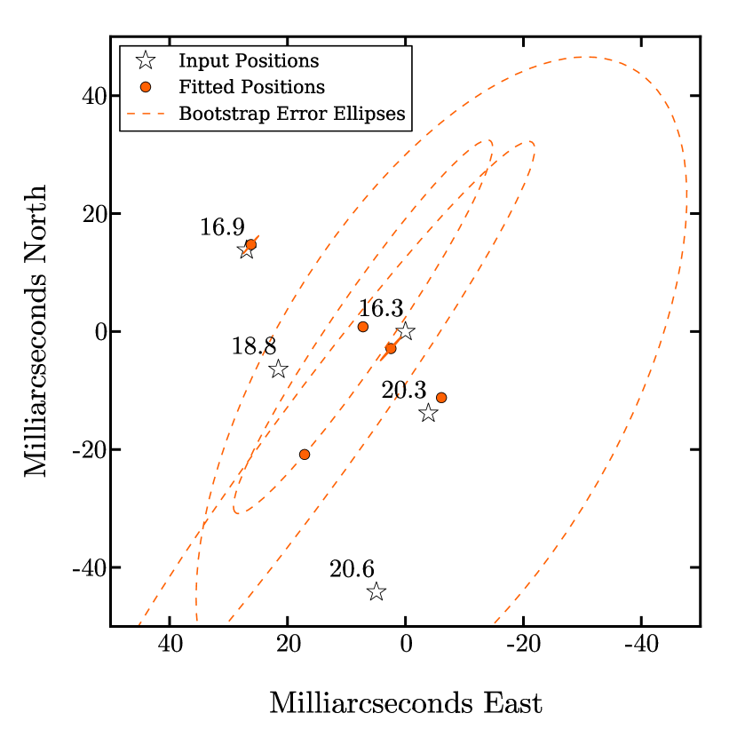
Figure 5: One epoch of the orbiting star field Field1 (white star symbols). Our recovered positions and astrometric error ellipses are also plotted (orange symbols). Only the positions of Sgr A* and Star 1 are accurately recovered. The positions of the fainter sources are not recovered. We have plotted the error ellipses of these sources using a dashed line. Note that these dashed curves are error ellipses, and not orbits.

Figure 6 shows the fitted position for Sgr A* and Star 1 for all 12 nights of observing Field1. The fainter stars have not been plotted because their positions are not recovered by the fitter. The astrometric residuals for Sgr A* and Star 1 are shown in the right panel of Figure 6. The astrometric precision in our fits can be estimated in three ways. First, we are able to characterize the quality of fits by computing the true residuals (right panel of Figure 6). Second, by assuming no significant orbital motion over the three-day time period, the dispersion in fitted positions over consecutive nights provides a rough measure of the astrometric precision for each observing run. Lastly, in Figure 7 we show calculated error ellipses generated using a standard bootstrapping algorithm.

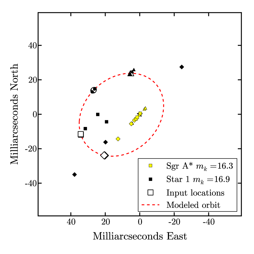
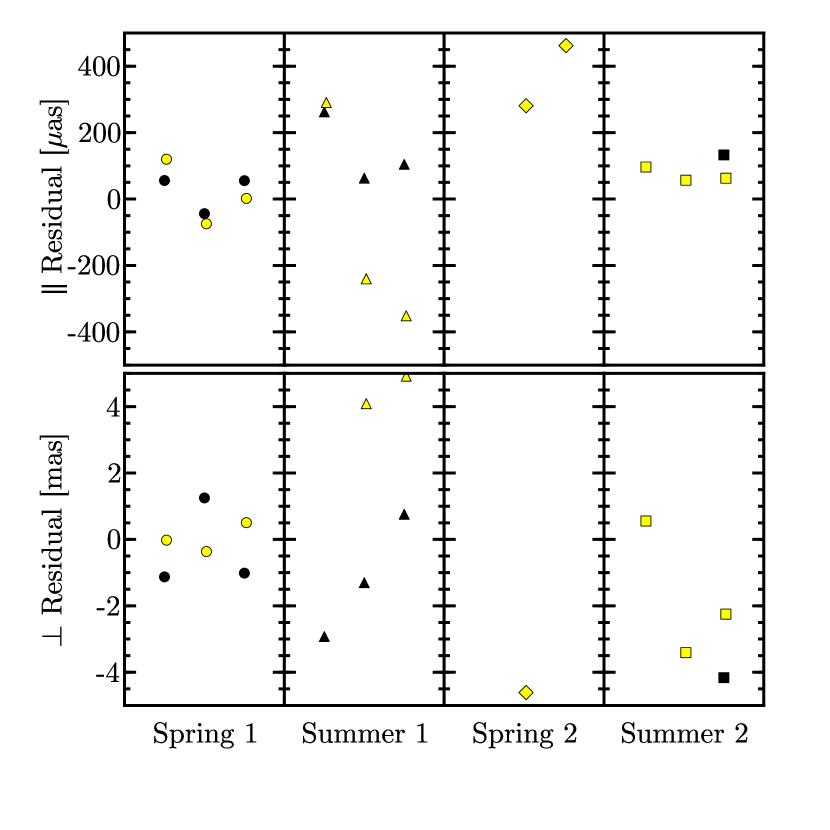
Figure 6: Left: We show the recovered positions of Sgr A* (yellow symbols) and Star 1 (black symbols) for four three-night runs of simulated Keck Interferometer data. The fits from each run are plotted with a unique symbol shape. The input orbit of Star 1 is also plotted (red dashed line) together with the expected location of Star 1 for each epoch (larger white symbols). Right: The astrometric residuals along the average baseline direction (top row) and the perpendicular direction (bottom row). Note the change from microarcseconds in the top row, to milliarcseconds in the bottom row.

Bootstrapping randomly re-samples the data, with replacement, several times and re-runs the fitter on each new sample. The process of drawing and replacing ensures that for most resampled data sets some of the data is redundant and some of the original data is missing. When our source fitter is run on the re-sampled data sets, a range of fitted parameter values are returned. The spread in the returned parameter values defines the shape of the uncertainty ellipses.

In Figure 7 we split the recovered positions shown in the left panel of Figure 6 into two plots, the left showing the results from the first year and the right plot showing the results from the second year of observation. We also show the astrometric error ellipses derived via our bootstrapping routine. As expected based on the shape of the Keck Interferometer PSF (Figure 1), our ability to accurately recover the position of the star depends on the position angle between the star and Sgr A*. During the first year (left panel of Figure 7), Star 1 is well separated in the direction of the baseline from Sgr A* and the astrometric residuals are $\sim 100\mu$as along the baseline direction and $\sim 4$mas in the perpendicular direction. In the second year (right panel) when Star 1 and Sgr A* are not well separated in the direction of the interferometer baseline, our astrometry is poor as indicated by the larger spread in fitted positions over the three-night runs, the larger residuals, and the significantly larger error ellipses derived for the epochs shown in 7. This is due, as discussed above, to overlapping sidelobes. The distinct shape of the bootstrap error ellipses which are much narrower in the direction of the interferometer baseline than in the direction perpendicular, reflects the shape of the Keck Interferometer PSF which has similar features.

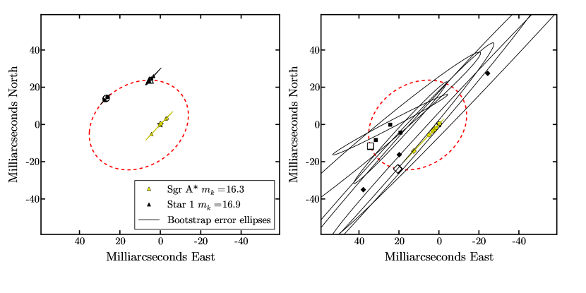
Figure 7: We have split the left panel of Figure 6 into two parts showing the recovered positions from the first year of data in the left panel, and the recovered positions for the second year of data in the right panel. Astrometric uncertainties for each fitted point are indicated with a solid line. Due to the large sidelobes in the Keck Interferometer PSF (Figure 1) our recovered positions are most precise when Star 1 and Sgr A* are well separated along the direction of the interferometer baseline.

We adopt the same observing program as for Field1, namely four three-night runs over two years for our simulated observations of Field2. Our fit to one night’s data is shown in Figure 8. We recover the position of Sgr A* and Star 1 but we are unable to recover the positions of the fainter stars.

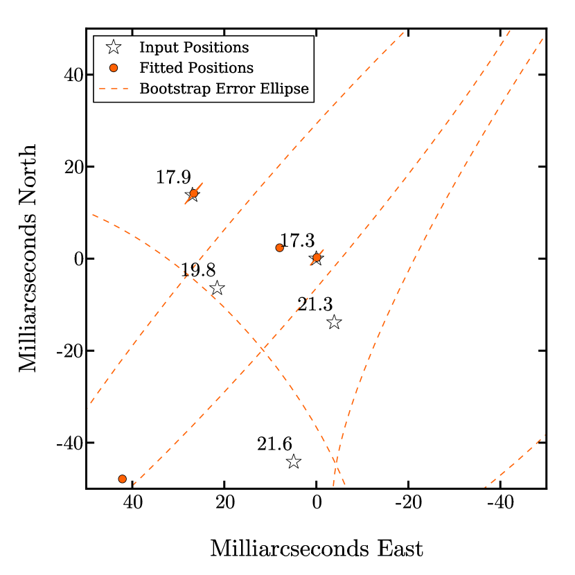
Figure 8: This plot is the same as Figure 5 but for Field2. We are unable to recover the positions of the fainter stars. The astrometric error ellipses for the unrecovered sources are plotted as dashed lines; note that these are not orbits.

Figure 9 shows our fitted positions for Sgr A* and Star 1 for each of the 12 nights of observing Field2. As is the case for Field1, our ability to recover the positions of Sgr A* and Star 1 is hindered when the sidelobes of each source overlap in the Spring and Summer of the second year. In Figure 10 we split the left panel of Figure 9 into two panels, showing the data from each year separately. For the observations during the first year our astrometric residuals on Sgr A* ($m_{K}=17.3$) and Star 1 ($m_{K}=17.9$) are $\sim 200~{}\mu$as along the baseline direction and $\sim 4~{}\mathrm{mas}$ in the perpendicular direction (first two columns in the right panel of Figure 9).

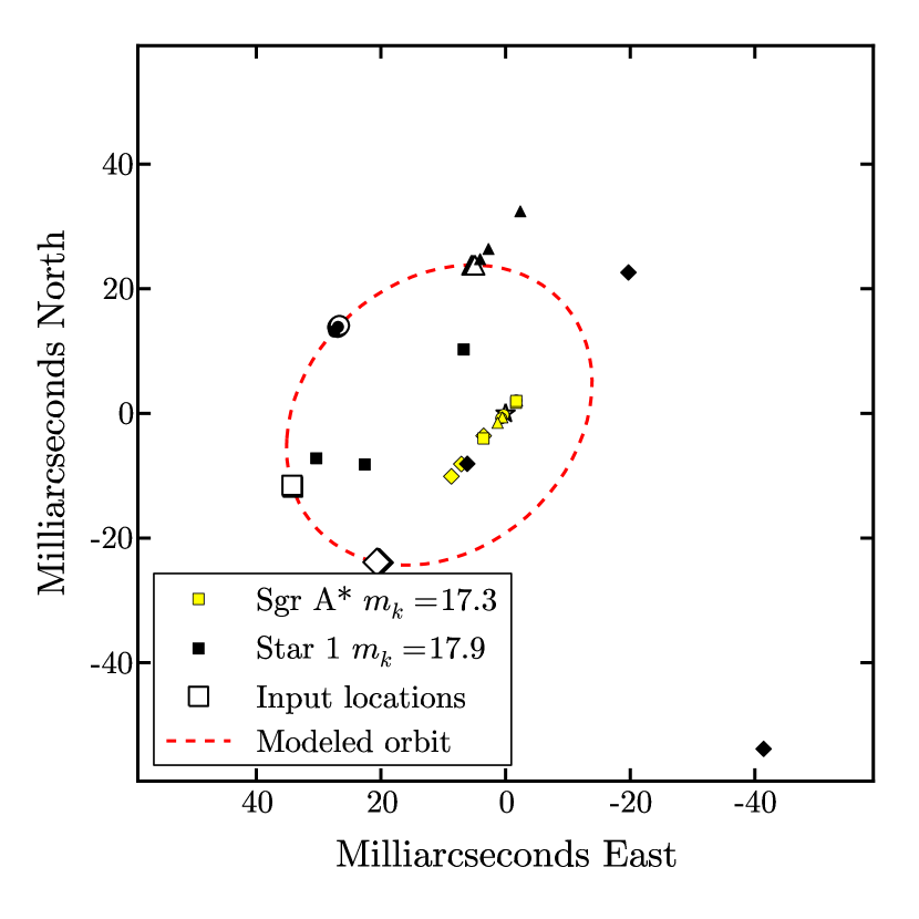
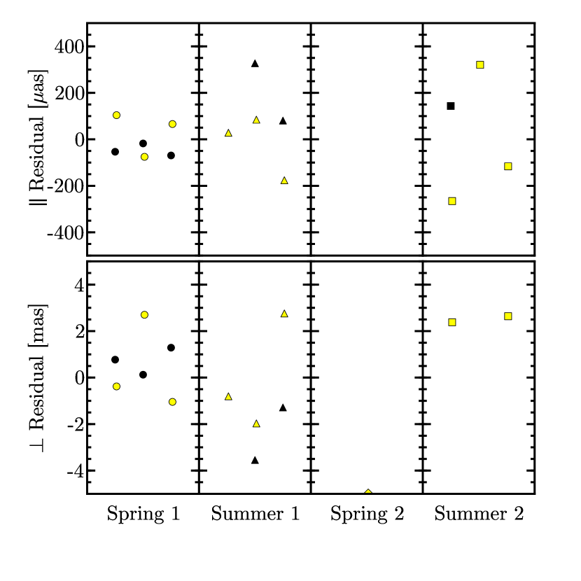
Figure 9: Left: Our recovered astrometric positions for each night of observing Field2. Black symbols represent Star 1 recovered positions, and yellow symbols refer to Sgr A* recovered positions. Symbol shapes are unique to each of the four three-day observing runs. Right: The astrometric residuals for each night are shown. Along the baseline direction the residuals are plotted in microarcseconds, while in the perpendicular direction they are plotted in milliarcseconds.

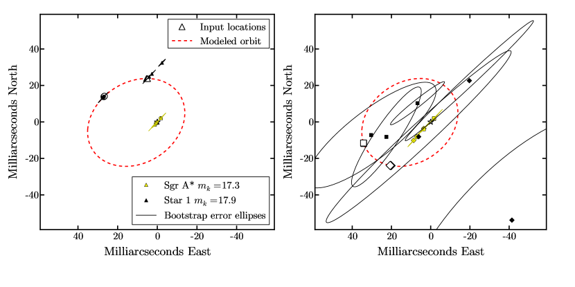
Figure 10: In this plot we split the left panel of Figure 9 showing the data from the first year in the left plot, and the data from the second year in the right plot. Black symbols still refer to Star 1 recovered positions, and yellow symbols refer to Sgr A* recovered positions. The symbol shapes designate the observing run in the same way as in Figure 9. Solid curves indicate the astrometric uncertainty. As discussed, our astrometry is worse in the second year due to overlapping sidelobes.

To generate a complete picture of why we are unable to recover the fainter sources, we investigate: 1) the signal-to-noise ratio of each source; and 2) source confusion, which incorporates source density and source contrast.

In Table 4 we show an upper limit to the signal-to-noise ratio for each source in Field1. To compute the values in Table 4 we made some simplifying assumptions to help elucidate some of the issues without the application of a more opaque formal treatment. Namely, we assume that there is no flux attenuation from the optical fiber and that each source is the only source present in the field. These two assumptions imply that our signal-to-noise ratios are strict upper limits. For example, a source with a reported upper limit to the signal-to-noise ratio of 10 or greater may provide no detectable signal in the presence of photon noise from brighter nearby sources or if the signal of an-off-axis source is attenuated by the optical fiber response. Additionally, including only one source in the field assumes a maximum visibility amplitude. With multiple sources in the field the fringe signal is diminished and the signal-to-noise ratio of the fringes of the more complex star field will be similarly reduced. In the limit of a crowded and complex star field, even large values in Table 4 do not necessarily imply a high signal-to-noise in simulated data. However, small values do ensure non-detections.

We list signal-to-noise values for each source with and without injection fluctuations. The large change in the upper limit to the signal-to-noise ratio when injection fluctuations are included indicate that they introduce a large source of noise. Since even the upper limits indicate a marginal signal-to-noise ratio for Stars 3 and 4, these sources are likely undetectable in the presence of the brighter sources included in our actual simulated data.

Table 4: Keck simulated data signal to noise for each spectral channel for Field1

Spectral Channel	Sgr A* ($m_{K}=16.3$)	Star 1 ($m_{K}=16.9$)	Star 2 ($m_{K}=18.8$)	Star 3 ($m_{K}=20.3$)	Star 4 ($m_{K}=20.6$)
Without injection fluctuations
2.00 microns	246	164	30	7	6
2.09 microns	242	146	26	6	5
2.18 microns	220	120	21	5	4
2.28 microns	200	94	17	4	3
2.38 microns	230	172	32	8	6
With injection fluctuations
2.00 microns	81	77	29	7	6
2.09 microns	81	75	25	6	4
2.18 microns	80	70	21	5	4
2.28 microns	78	64	16	4	3
2.38 microns	80	78	30	8	6

Note. — This table shows the simulated signal-to-noise values for the sources in Field1. As discussed in the text these values are upper limits and are included here to give a rough feeling of the sensitivity limits. Injection fluctuations dominate the noise for the brighter sources while background and readnoise are significant for the fainter sources. As a convenience, we include the simulated signal-to-noise ratio constructed without any injection fluctuations for reference.

Table 5, like Table 4 for Field1, illustrates our upper limits to the signal-to-noise ratio simulated for each source in Field2. Even the upper limits on the signal-to-noise ratio indicate that no real signal is detected for Stars 3 and 4.

Table 5: Keck simulated data signal to noise for each spectral channel for Field2

Spectral Channel	Sgr A* (k=17.3)	Star 1 (k=17.9)	Star 2 (k=19.8)	Star 3 (k=21.3)	Star 4 (k=21.6)
Without injection fluctuations
2.00 microns	108	70	12	3	2
2.09 microns	103	61	10	3	2
2.18 microns	91	48	9	2	2
2.28 microns	82	39	7	2	1
2.38 microns	102	73	13	3	2
With injection fluctuations
2.00 microns	68	55	12	3	2
2.09 microns	67	49	11	3	2
2.18 microns	64	42	9	2	2
2.28 microns	60	36	7	2	1
2.38 microns	67	56	13	3	3

Note. — Simulated upper limits to the signal-to-noise ratio for each source in Field2.

As we discussed in Section 3.4 the sidelobes of the Keck Interferometer PSF will impose a confusion limit in the Keck Interferometer data both because the lobes will set a contrast limit and because they will tend to overlap when sources are not well separated. In Figure 11 we show the 1% (red), 10% (green), and 50% (blue) contours of the Keck Interferometer PSF. We also plot the fiber response function and the orbital path of one of our stars. This plot shows that detecting a faint source will be easiest when the star enters a region where the sidelobe flux from Sgr A* is lowest. However, there is the competing factor of the fiber response function which tends to attenuate the flux from sources which are located far from the center of the field. Thus while there are some regions in the field beyond the 1% contours of the PSF, detecting a source there is made difficult by the low transmission of the fiber.

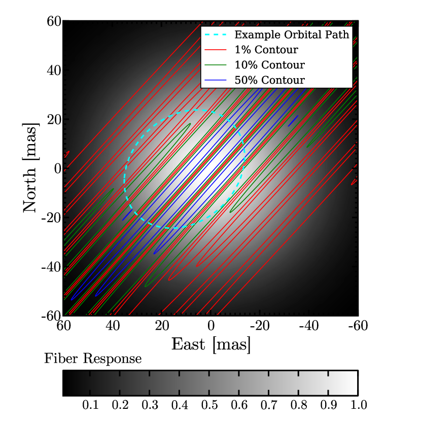
Figure 11: In order to illustrate some of the difficulties in detecting a stellar source in orbit about Sgr A* we overplot one of our adopted stellar orbits (cyan dashed curve) on top of the Keck Interferometer PSF (solid red, green, and blue contours at 1%, 10%, and 50% power respectively). We also show the optical fiber response in grayscale.

An independent limit distinct from contrast but prominent in confusion noise is source crowding. In an attempt to isolate the effects of crowding and provide evidence of whether crowding is limiting all the previous fits, we also simulate data for four star fields, each with a different number of $m_{K}=17$ stars. These simulations also provide some insight into the potential performance of the Keck Interferometer if the KLF at the Galactic Center is significantly flatter than Field1 or Field2. The four panels of Figure 12 show our fits to these star fields. The star fields were constructed as follows: First, one source with $m_{K}=16.3$ is placed at the origin and another with $m_{K}=17.0$ is placed randomly within a 100 x 100 milliarcsecond field (panel one). To this star field, an additional $m_{K}=17.0$ source is placed randomly in the field (panel two), and so on until a total of four $m_{K}=17.0$ sources are present in addition to the central $m_{K}=16.3$ magnitude source (panels 3 and 4).

In panel one of Figure 12, our fits to the simulated visibility data recover the input positions of both sources. Our confidence in these fits is implied by the small error ellipses generated by our bootstrapping routine. In panel two, a second $m_{K}=17$ magnitude source has been added to the star field beyond the half-maximum radius of the optical fiber attenuation function. Note that due to the fiber function, the flux of the unrecovered star is attenuated by $\sim 1$ magnitude. We are still able to recover the positions of the first two sources but we cannot recover the position of this third source due mostly to the increased contrast caused by the fiber-function-attenuated flux. In the third panel, a third $m_{K}=17$ magnitude source is added to the field, this time very near the origin. Our fits to this field do recover the positions of the three sources within the half-maximum radius of the fiber function with some confidence; the star placed outside this radius is still not recovered.

The accuracy and the precision of the recovered source positions in panel 3 are somewhat degraded compared to the recovered positions in panels 1 and 2. This degradation in precision is due to the increased crowding of the field with relatively bright sources and the effects of overlapping sidelobes. In the fourth panel of Figure 12, with 5 bright sources in the field, the effects of overlapping sidelobes are so severe that we cannot recover the position of any source.

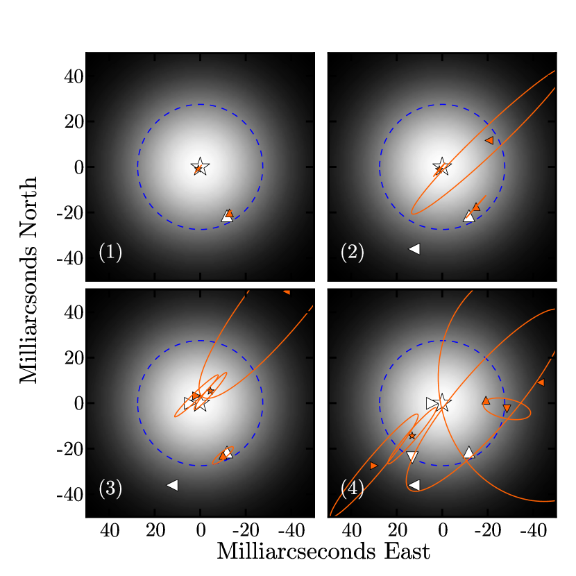
Figure 12: In these panels our recovered positions (orange symbols) and error ellipses are plotted showing our performance recovering source positions from Keck Interferometer data when more and more sources are present. The input star field for each panel includes Sgr A* at the origin with $m_{K}=16.3$ (star symbol). In addition to Sgr A* each star field also includes from 1 to 4 $m_{K}=17$ stars (isosceles triangles with vertices pointing up, right, left, and down corresponding to the first, second, third and fourth added star respectively). Also plotted is the Gaussian fiber response function (grayscale) and the 50% contour of this function (blue dashed line). Source fluxes are attenuated by this function before detection.

5.2 Star Fields Observed with GRAVITY

Figure 13 shows the recovered positions for Sgr A*, Star 1, and Star 2 for four three-night observing runs following the same schedule that was used for the Keck simulations. The astrometric residuals (shown in the right panel of Figure 13) are $\sim 10~{}\mu$as, $\sim 100~{}\mu$as, and $\sim 200~{}\mu$as for Sgr A*, Star 1, and Star 2 respectively. In Figure 14 we also show the bootstrap error ellipses associated with our fitted positions; where none are seen they are smaller than the plotting symbols. Stars 3 and 4 are not plotted because their positions are not well recovered.

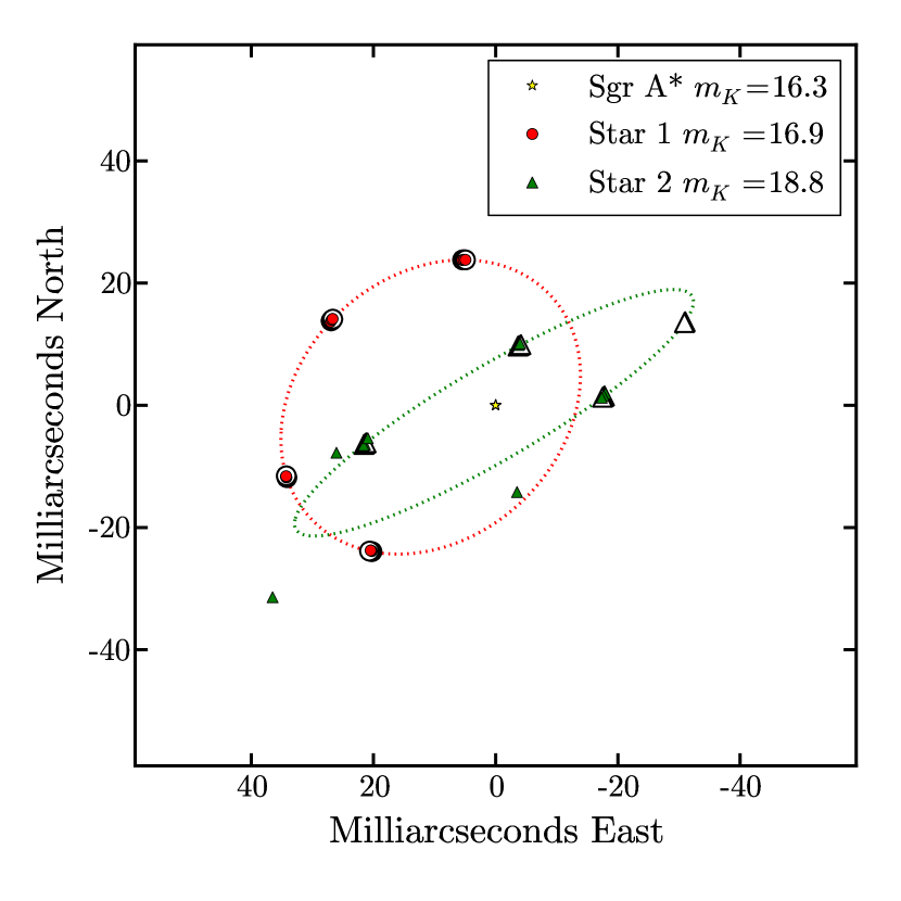
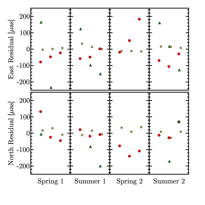
Figure 13: This plot is similar to Figure 6 but shows the results for our GRAVITY simulations. Left: The recovered positions of Sgr A* (yellow star symbols), Star 1 (red circle symbols), and Star 2 (green triangle symbols) for 12 nights of simulated GRAVITY data. The input orbits of Star 1 and Star 2 are also plotted (red and green dashed lines respectively). White symbols show the input location for each source. Note that in our GRAVITY plots, symbol shape is used to identify sources, not observing epoch. Right: The astrometric residuals in the North and East directions are plotted for both Sgr A*, Star 1, and Star 2.

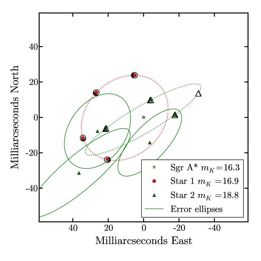
Figure 14: The left panel of Figure 13 but here we include the bootstrap error ellipses. Where ellipses cannot be seen they are smaller than the plotting symbols. White symbols indicate input locations.

For one run, when Star 2 is farthest from the center of the field, we are unable to recover its position on any of the three nights. The optical fiber transmission function attenuates the flux most during this run. We investigate some of the limiting factors to recovering source positions in GRAVITY data below.

Figure 15 shows our results fitting to simulated GRAVITY data of Field2. We plot only the fitted positions for Sgr A* and Star 1 because no other sources were confidently recovered. At input magnitudes of $m_{K}=17.3$ and $m_{K}=17.9$, our astrometric residuals for Sgr A* and Star 1 are $\sim 50\mu$as and $\sim 150\mu$as respectively.

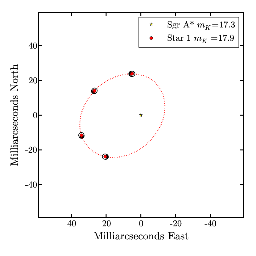
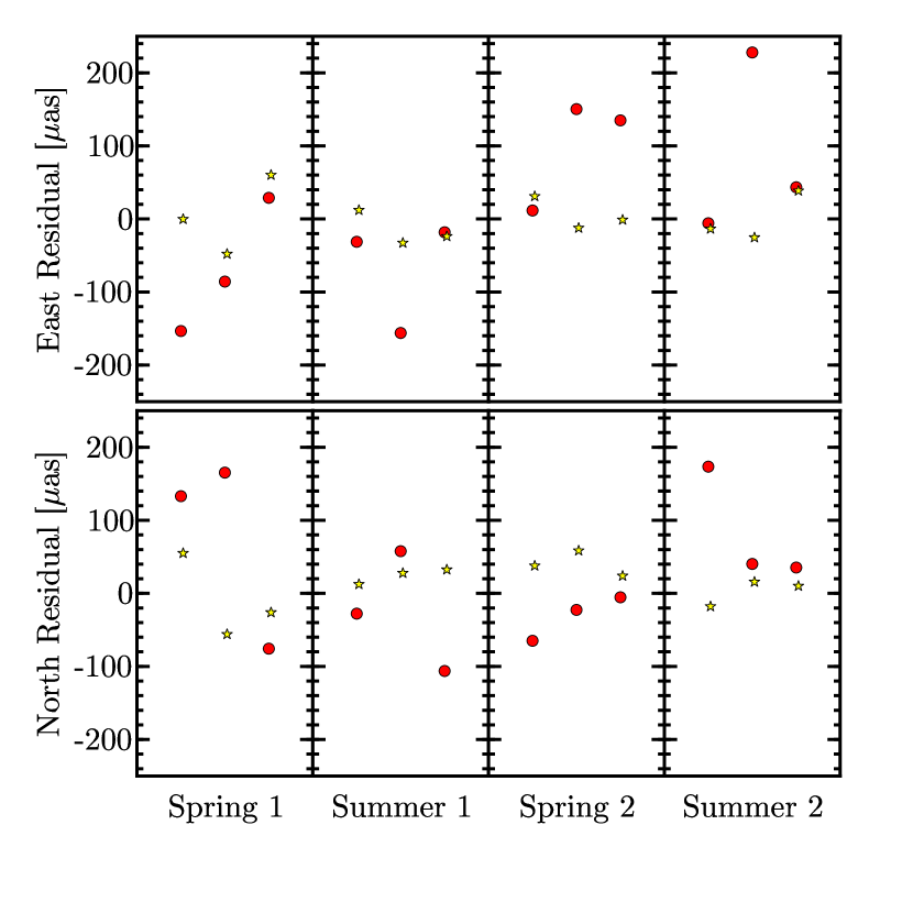
Figure 15: This plot is the same as Figure 13 but for Field2. In this case only the positions of Sgr A* and Star 1 are recovered. Error ellipses are plotted for each point. White symbols indicate input locations.

To evaluate the limiting factors in our GRAVITY observations, we run diagnostic tests similar to those we perform for our ASTRA simulations. We start by calculating upper limits to the signal-to-noise ratio of each source. Each fringe generated by GRAVITY will have less photons than the corresponding observation with ASTRA at the Keck Interferometer. First, because GRAVITY combines the light from four telescopes between six baselines, only $\frac{2}{3}$ of the flux incident on each aperture is available for combination. Second, the individual apertures at the VLTI are smaller than the apertures at Keck. Finally, the transmission of the GRAVITY instrument is expected to be less than the transmission of ASTRA at Keck.

Table 6 shows upper limits to the signal-to-noise ratio in our GRAVITY simulations calculated for each source in Field1. We see that for the brightest sources, where injection fluctuations dominate the noise at Keck, GRAVITY will provide a higher signal-to-noise ratio because with 6 baselines, the effect of injection fluctuations averages down. For fainter sources, GRAVITY will provide a lower signal-to-noise because, as mentioned above, the light is split more ways and the transmission is lower. Table 6 indicates, even with upper limits to the signal to noise, that Stars 3 and 4 will not be detectable in our simulations.

Table 6: VLTI simulated signal-to-noise ratios for each spectral channel for Field1

Spectral Channel	Sgr A* (k=16.3)	Star 1 (k=16.9)	Star 2 (k=18.8)	Star 3 (k=20.3)	Star 4 (k=20.6)
2.00 microns	101	74	12	3	2
2.09 microns	109	69	10	3	1
2.18 microns	102	58	9	4	3
2.28 microns	92	50	9	3	1
2.38 microns	82	40	6	1	1

Note. — This table shows upper limits to the simulated signal-to-noise ratio of each source in Field1 provided by our model of the VLTI GRAVITY instrument.

Table 7 shows upper limits to the signal-to-noise ratios for the sources in Field2. These ratios indicate that no detectable signal is present from Stars 2, 3, and 4 in Field2.

Table 7: VLTI simulated signal-to-noise ratios for each spectral channel for Field2

Spectral Channel	Sgr A* (k=17.3)	Star 1 (k=17.9)	Star 2 (k=19.8)	Star 3 (k=21.3)	Star 4 (k=21.6)
2.00 microns	43	30	4	2	0
2.09 microns	43	30	4	1	0
2.18 microns	42	26	3	0	0
2.28 microns	36	18	1	1	1
2.38 microns	33	16	1	0	1

Note. — This table shows simulated upper limits to the signal-to-noise ratio of each source in Field2 provided by our model of the VLTI GRAVITY instrument.

In Figure 16, we see that our ability to accurately detect and track stars in the vicinity of Sgr A* will depend on the exact location of the star. For example, within $~{}25$ mas of Sgr A*, where the optical fiber transmits light most strongly, the PSF is at or above the 1% level. Thus, as in the Keck case discussed above, there is a tug-of-war of considerations affecting the detectability of a source in the vicinity of Sgr A*. Faint sources are more easily detected outside of the 1% contours of the PSF. Because of the fiber attenuation function, when sources are far from the center of the field their flux level is likely to drop below the detection limit ($m_{K}\sim 19$ in six hours).

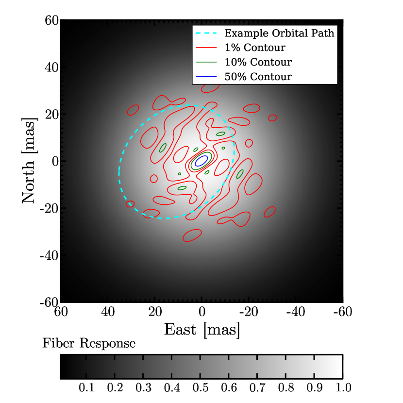
Figure 16: This figure is the same as Figure 11 but shows the GRAVITY PSF (red, green, and blue contours at 1%, 10%, and 50% respectively). In addition, the fiber response function (grayscale) and an example stellar orbit (cyan dashed line) are also plotted.

While more beam splits reduce the number of photons combined between each pair of telescopes at VLTI, the trade off is significantly increased uv-coverage. In fact, the confusion limit for GRAVITY will be better than for ASTRA at Keck. In Figure 17, as in Figure 12 for the ASTRA, we attempt to isolate the contribution of source crowding to the confusion noise by observing star fields with more and more equal magnitude stars. As in Figure 12, we start with Sgr A* at $m_{K}=16.3$ and one star with $m_{K}=17$. We then add one $m_{K}=17$ star at a time until a total of four stars are in the field. Since the VLTI provides good uv-coverage of the Galactic Center, precise astrometry on even five bright sources within $\sim 50$ mas of Sgr A* is possible.

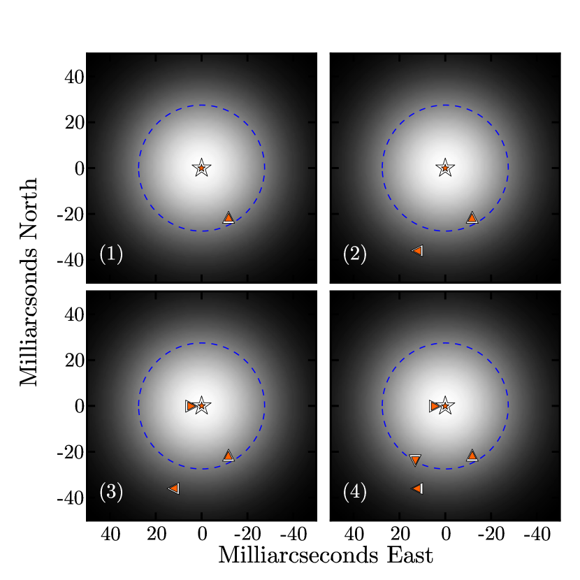
Figure 17: Our recovered positions (orange symbols) are plotted showing our performance recovering source positions from GRAVITY data when more and more sources are present. The input star field for each panel includes Sgr A* at the origin with $m_{K}=16.3$ (star symbol). In addition to Sgr A* each star field also includes from 1 to 4 $m_{K}=17$ stars (isosceles triangles with vertices pointing up, right, left, and down corresponding to the first, second, third and fourth added star respectively). Bootstrap error ellipses are smaller than the plotting symbols. Also plotted is the Gaussian fiber response function (grayscale) and the 50% contour of this function (blue dashed line). Source fluxes are attenuated by this function before detection.

Since Table 6 indicates that GRAVITY will be unable to recover Stars 3 and 4 due to inadequate signal-to-noise, we also tested the performance on a brighter star field labeled Field0. Field0 is identical to Field1 but with the flux of each source increased by one magnitude. Our fits are plotted in Figure 18. We are again able to recover the positions Sgr A*, Star 1 and Star 2 for three out of four runs. During the run when Star 2 is farthest off axis we again run into some difficulty, because our fitter interchanges Star 2 and Star 3. This is due to the effects of the fiber response function which attenuates the flux from Star 2 most during this run while Star 3 remains at a nearly constant brightness near the center of the field. The interchange is a result of our iterative fitting algorithm. This interchange does not affect the results of multi-epoch observations which can track the sources and identify the switch.

Star 3 in Field0 is recovered only less than half of the time, indicating that the star is only marginally detectable in the data and suggesting a sensitivity limit around $m_{K}\sim 19$. Even so, these results imply the potential to detect and monitor several moderately bright sources within $\sim 50$ mas of Sgr A* should they exist.

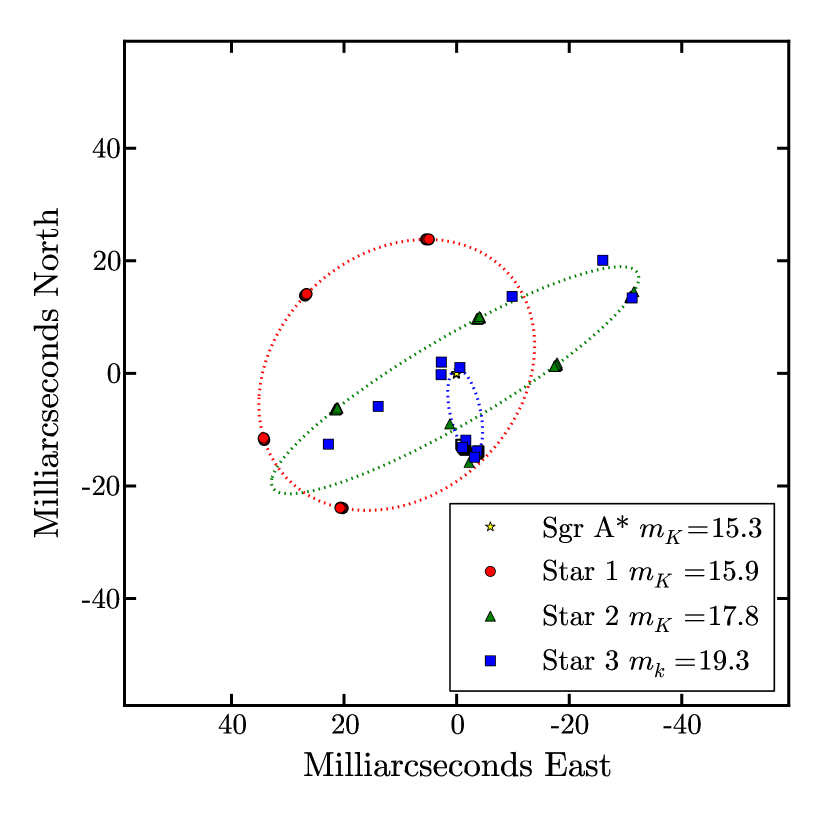
Figure 18: Here we show our fits to 12 nights of simulated GRAVITY data for Field0. Some difficulty in deducing the position of Star 2 occurs when it is farthest off axis. During these nights, the flux of Star 2 is most attenuated by the fiber response. Since Star 3 is located close to on-axis for all epochs, it appears as similarly bright to Star 2 during these nights. For two nights during this run, our fitter has interchanged Star 2 and Star 3.

6 Discussion

In Section 5, our Keck Interferometer ASTRA simulations show the ability to detect and track a stellar source on an orbit within $\sim 50$ mas of Sgr A* with a single baseline interferometer. This performance depends on the source contrast and position angle with respect to Sgr A*. However, we demonstrate the potential to detect and track an $m_{K}\sim 18$ star when Sgr A* is at $m_{K}=17.3$ and the star and Sgr A* are well separated along the baseline direction (left panel of Figure 10). We show that $\sim 150~{}\mu$as astrometry is possible along the baseline direction and $\sim 3$ mas precision is possible in the transverse direction during unconfused epochs. Our precision improves if the sources are brighter. Since a single baseline interferometer produces an extended PSF, confusion still affects our ability to accurately detect and track sources when their sidelobes overlap.

While at first glance ASTRA seems quite limited compared to GRAVITY in its ability to detect and track stars within $\sim 50$ mas of Sgr A*, we show that the single baseline instrument could significantly contribute to the Galactic Center science case. Specifically, we show that multi-epoch observations have the ability to distinguish whether the region contains no bright sources, one or two bright sources, or several bright sources (see Figures 7, 10, and 12). Since the source content in the region is truly unknown, any additional information about the stellar density near the Galactic Center would be quite valuable. New information could inform, for example, dynamical theories of the nuclear cluster which must explain the positions of the stars. Further, the higher throughput, larger apertures, and fewer beam splits provide a larger signal in the ASTRA fringes (compare for example Tables 5 and 7). While confusion noise will constrain ASTRA observations, if no star brighter than $m_{K}\sim 19$ exists in the field ASTRA may have an advantage in making a detection. Because ASTRA is currently capable of making these observations the potential exists to provide the community with some constraints before GRAVITY comes online at the VLTI and before ASTRA operations cease at Keck.

While long-term operations of ASTRA are not currently planned, we note that if ASTRA and GRAVITY observations could be obtained contemportaneously, some importvement in the recovery of faint sources may be possible. In simulations where we combined ASTRA and GRAVITY data (using the assumptions in Table 3 for each instrument), we found that we can recover the $m_{K}=19.8$ source in some epochs where it is not recovered using either ASTRA or GRAVITY data alone.

Our GRAVITY simulations show that that instrument will attain a lower confusion limit than ASTRA. This lower confusion in GRAVITY observations is due to the increased uv-coverage provided by the VLTI array. This makes it possible to detect and monitor multiple sources in the field. We demonstrate the potential for $\sim 10~{}\mu$as precision astrometry on Sgr A* at $m_{K}=16.3$ and $\sim 100~{}\mu$as precision astrometry on sources as faint as $m_{K}=18.8$ in six hours of observing our simulated star fields. However, we show that the decreased throughput at GRAVITY and the larger number of beam splits required to create six baselines will impose a detection limit at GRAVITY which will make it difficult to detect sources at $m_{K}\gtrsim 19$. In fact, we show that for one simulated three-night run using GRAVITY, we are unable to recover the position of the $m_{K}=18.8$ source. While this reflects contrast and fiber function issues to some extent, it shows that in real observations GRAVITY may struggle to detect sources at this brightness level.

GRAVITY’s ability to recover precise astrometry for multiple sources within $\sim 50$ mas from Sgr A* suggests it should be able to constrain the shape of an extended mass distribution at the Galactic Center(Rubilar & Eckart, 2001; Weinberg et al., 2005). Any model of the central structure must include the mass of the black hole and the mass and radial profile of an extended distribution of matter. To constrain these parameters and to break the first-order degeneracy between the retrograde precession due to the extended matter and the prograde precession attributable to General Relativity, multiple stars with distinct angular momenta will be needed (Rubilar & Eckart, 2001; Weinberg et al., 2005). Since the astrometric signal of orbital precession increases linearly with the number of revolutions, monitoring stars on short-period orbits within $\sim 50$ mas is preferred, since a larger signal can be detected in shorter time.

Our GRAVITY simulations also demonstrate the astrometric precision needed to detect relativistic effects on stellar orbits. Our simulated performance of $\sim 100~{}\mu$as suggests that low order effects of relativity, such as the prograde precession, will be detectable (Weinberg et al., 2005). However, higher order relativistic effects, such as detecting the influence of the black hole spin on stellar orbits, will be more difficult, requiring measurements more precise than those demonstrated here(Weinberg et al., 2005; Merritt et al., 2011).

A recent paper by Vincent et al. (2011) modeled the imaging mode astrometric performance of GRAVITY, applying the CLEAN algorithm to images formed using the interferometric visibilities. In that paper, the authors mainly investigate the astrometric precision attainable on Sgr A* when it is very bright. They compare their performance after a whole night of observing to individual 100 second exposures. They show that $\sim 40~{}\mu$as precision is attainable on Sgr A* in 100 seconds when it is very bright and the field is simple. Our simulations show that astrometric precision on the order of the angular extent of the inner-most stable circular orbit of the black hole ($\sim 30~{}\mu$as) is attainable on Sgr A* even in the midst of our more complicated star field. However, $\sim 10~{}\mu$as precision is attained after 6 hours of observing; time resolved astrometry in our fields will necessarily be less precise. Not only are shorter observations less sensitive to sources in the field, but with less time spent on-source the uv-coverage is reduced. Both of these effects combine to degrade the astrometric precision by decreasing the signal-to-noise ratio and increasing the confusion. We demonstrate that as astrometry on Sgr A* becomes more difficult due to confusion with bright stars in the small field, astrometry on those bright stars becomes easier. Thus GRAVITY should provide some traction on investigating General Relativistic effects, either through observations of Sgr A* itself given a faint star field or by tracking stars in the vicinity of Sgr A* given a brighter star field.

Although our simulations did not include Sgr A* variability explicitly, variability could provide an interesting paradigm for making these observations. During high states, we will be able to conduct precise astrometry of Sgr A*, anchoring our field. During low states, the decreased contrast will provide an opportunity to probe for fainter stellar sources in the region. This back-and-forth approach could be harnessed to precisely monitor faint sources. To demonstrate these effects, we ran our simulator with Sgr A* set to very low brightness but with the star field magnitudes kept constant. During these runs, we were able to recover stellar positions more easily, since confusion with Sgr A* was reduced. On the other hand, a very bright Sgr A* is easily detected with a high level of precision. The timescales of Sgr A* variability are conducive to seeing both high and low states while observing. Flares are observed on timescales of $\sim 10-100$ minutes and Sgr A* often changes flux by more than one magnitude.

7 Summary and Future Work

Our simulations demonstrate that ASTRA and GRAVITY will be able to provide different insights into the star field near Sgr A*. The Keck instrument will excel if the inner $\sim 50$ mas is a simple field, with a steep luminosity function including at least one relatively bright star. We demonstrate the ability to recover a source with $m_{K}=17.9$ in a field with other similarly bright sources and we show in Table 5 that a source as faint as $m_{K}=19.8$ might be detected if the star field is faint and the visibility amplitude is high. Multi-epoch observations will be necessary to mitigate source confusion as the astrometry will be most precise when the star orbits through position angles where the astrometric offset along the projected baseline direction is large. GRAVITY’s sensitivity to sources will not depend strongly on orbital phase as is the case with ASTRA since GRAVITY provides a more symmetric PSF. Moreover, GRAVITY will be better able to track orbits if the stellar field has a shallower luminosity function, as it is not as affected by confusion noise and because it will have difficulty detecting sources fainter than $m_{K}\sim 19$.

The minimal uv-coverage provided by the single baseline of the Keck Interferometer, which is furthermore situated in the northern hemisphere where Sgr A* transits low, is not insufficient for providing valuable information for scientific advance. In fact, we demonstrate the ability to detect and monitor stars when there is sufficient astrometric offset along the baseline direction. These results could be extended to infer the performance of a single baseline of the VLTI. Given the technical and practical challenges of using all four VLT apertures to create six baselines, it is important to consider that even a reduced array at VLTI could make important contributions to Galactic Center science. Because the VLTI is situated in the southern hemisphere where Sgr A* transits high, even a single baseline of the VLTI would provide much more uv-coverage of Sgr A* than Keck. If no bright stars are detected in the region, then a reduced array could be used to provide more photons in each fringe, increasing the sensitivity of the interferometer at the expense of a more extended PSF, which would even so be less extended than the Keck Interferometer PSF we show above.

Moving forward, further GRAVITY simulations incorporating a variable Sgr A* and stars on post-Newtonian orbits will be useful in the interim before that instrument comes online. Such simulations will aid in predicting the challenges of characterizing the gravitational potential at the Galactic Center with stellar orbits and in creating the necessary analysis tools which will be needed for fitting the complicated orbits which are expected to be observed.

Finally, some interferometric observations of Galactic Center sources have been made at Keck and the VLTI (e.g., Pott et al., 2008b). Pott et al. (2008a) observed IRS 7 with the VLTI and showed it is suitable for use as a phase reference source; similar observations have been made with the Keck Interferometer. Dual field phase referencing has been demonstrated on-sky with ASTRA (Woillez et al. in prep), and the instrument is poised to observe the field around Sgr A*. An obvious next step is to actually observe Sgr A* and to search for real sources.

8 Aknowledgements

We would like to thank and aknowledge the Keck Interferometer ASTRA team for their work on the instrument and for valuable input in designing our simulator. JAE gratefully acknowledges support from an Alfred P. Sloan Research Fellowship.

References

- Colavita (1999) Colavita, M. M. 1999, PASP, 111, 111
- Colavita (2009) —. 2009, New A Rev., 53, 344
- Do et al. (2009) Do, T., Ghez, A. M., Morris, M. R., Yelda, S., Meyer, L., Lu, J. R., Hornstein, S. D., & Matthews, K. 2009, ApJ, 691, 1021
- Do et al. (2009) Do, T., Ghez, A. M., Morris, M. R., et al. 2009, ApJ, 703, 1323
- Dodds-Eden et al. (2011) Dodds-Eden, K., et al. 2011, ApJ, 728, 37
- Eckart et al. (1992) Eckart, A., Genzel, R., Krabbe, A., Hofmann, R., van der Werf, P. P., & Drapatz, S. 1992, Nature, 355, 526
- Eisenhauer et al. (2008) Eisenhauer, F., et al. 2008, in Society of Photo-Optical Instrumentation Engineers (SPIE) Conference Series, Vol. 7013, Society of Photo-Optical Instrumentation Engineers (SPIE) Conference Series
- Esposito et al. (2000) Esposito, S., Riccardi, A., & Femenía, B. 2000, A&A, 353, L29
- Fritz et al. (2010) Fritz, T., et al. 2010, MNRAS, 401, 1177
- Genzel et al. (2003) Genzel, R., et al. 2003, ApJ, 594, 812
- Ghez (2010) Ghez, A. 2010, in Dynamics from the Galactic Center to the Milky Way Halo
- Ghez et al. (2005) Ghez, A. M., et al. 2005, ApJ, 635, 1087
- Ghez et al. (2008) —. 2008, ApJ, 689, 1044
- Gillessen et al. (2009) Gillessen, S., Eisenhauer, F., Trippe, S., Alexander, T., Genzel, R., Martins, F., & Ott, T. 2009, ApJ, 692, 1075
- Gillessen et al. (2006) Gillessen, S., et al. 2006, in Society of Photo-Optical Instrumentation Engineers (SPIE) Conference Series, Vol. 6268, Society of Photo-Optical Instrumentation Engineers (SPIE) Conference Series
- Lane & Colavita (2003) Lane, B. F., & Colavita, M. M. 2003, AJ, 125, 1623
- Lawson (2000) Lawson, P. R., ed. 2000, Principles of Long Baseline Stellar Interferometry
- Merritt et al. (2011) Merritt, D., Alexander, T., Mikkola, S., & Will, C. M. 2011, Phys. Rev. D, 84, 044024
- Olling & Merrifield (2000) Olling, R. P., & Merrifield, M. R. 2000, MNRAS, 311, 361
- Pott et al. (2008a) Pott, J.-U., Eckart, A., Glindemann, A., Kraus, S., Schödel, R., Ghez, A. M., Woillez, J., & Weigelt, G. 2008a, A&A, 487, 413
- Paumard et al. (2006) Paumard, T., Genzel, R., Martins, F., et al. 2006, ApJ, 643, 1011
- Pott et al. (2008b) Pott, J.-U., Woillez, J., Wizinowich, P. L., Eckart, A., Glindemann, A., Ghez, A. M., & Graham, J. R. 2008b, in Society of Photo-Optical Instrumentation Engineers (SPIE) Conference Series, Vol. 7013, Society of Photo-Optical Instrumentation Engineers (SPIE) Conference Series
- Reid et al. (2009) Reid, M. J., et al. 2009, ApJ, 700, 137
- Rubilar & Eckart (2001) Rubilar, G. F., & Eckart, A. 2001, A&A, 374, 95
- Schödel et al. (2002) Schödel, R., et al. 2002, Nature, 419, 694
- Shao & Colavita (1992) Shao, M., & Colavita, M. M. 1992, A&A, 262, 353
- Vincent et al. (2011) Vincent, F. H., Paumard, T., Perrin, G., Mugnier, L., Eisenhauer, F., & Gillessen, S. 2011, MNRAS, 412, 2653
- Weinberg et al. (2005) Weinberg, N. N., Milosavljević, M., & Ghez, A. M. 2005, in Astronomical Society of the Pacific Conference Series, Vol. 338, Astrometry in the Age of the Next Generation of Large Telescopes, ed. P. K. Seidelmann & A. K. B. Monet, 252–+
- Woillez et al. (2010) Woillez, J., et al. 2010, in Society of Photo-Optical Instrumentation Engineers (SPIE) Conference Series, Vol. 7734, Society of Photo-Optical Instrumentation Engineers (SPIE) Conference Series
- Woillez et al. (2012) Woillez, J., et al. 2012, PASP, 124, 51