Escape Dynamics in the Discrete Repulsive $\phi^{4}$-Model

Abstract

We study deterministic escape dynamics of the discrete Klein-Gordon model with a repulsive quartic on-site potential. Using a combination of analytical techniques, based on differential and algebraic inequalities and selected numerical illustrations, we first derive conditions for collapse of an initially excited single-site unit, for both the Hamiltonian and the linearly damped versions of the system and showcase different potential fates of the single-site excitation, such as the possibility to be “pulled back” from outside the well or to “drive over” the barrier some of its neighbors. Next, we study the evolution of a uniform (small) segment of the chain and, in turn, consider the conditions that support its escape and collapse of the chain. Finally, our path from one to the few and finally to the many excited sites is completed by a modulational stability analysis and the exploration of its connection to the escape process for plane wave initial data. This reveals the existence of three distinct regimes, namely modulational stability, modulational instability without escape and, finally, modulational instability accompanied by escape. These are corroborated by direct numerical simulations. In each of the above cases, the variations of the relevant model parameters enable a consideration of the interplay of discreteness and nonlinearity within the observed phenomenology.

I Introduction

The escape problem for systems of coupled objects.

The escape problem for single particles of coupled degrees of freedom or for small chains of coupled objects, concerns their exit from the domain of attraction of a locally stable state Hanggi0 ; Hanggi . Its investigation is crucial for the understanding of evolutionary processes in natural sciences, representing the transition from a stable state to another, or to extinction and collapse.

Transition state theory deals exactly with this kind of problem by referring to the case where the considered objects, initiating from the domain of attraction of a locally stable state, escape to a neighboring stable state crossing a separating energy barrier. A natural example of this sort involves a bistable potential, where the barrier corresponds to the height of the saddle point separating the two minima of the potential. This mechanism has been widely explored in numerous physical settings, including (but not limited to) phase transitions, chemical kinetics, pattern formation and the kinematics of biological waves – see, e.g., Refs. PF ; KMI ; YN ; AS and references therein. Depending on the geometry of the underlying potential energy landscape which may possess multiple minima, topological excitations with a “kink shape” (which can be thought of as instantons) interpolating between the adjacent minima may exist and play a critical role in the study of transition probabilities.

Another example of such an escape process is the one whereby the considered objects, initiating within the basin of attraction of a locally stable state, escape towards infinity. This process is often termed collapse and it is associated with the emergence of finite time singularities for the corresponding dynamical system. Collapse or blow-up in finite time is quite widespread as an instability mechanism in diffusion processes and wave phenomena in nonlinear media bb ; souplet ; bs ; susu ; ws . Generally, the collapse phenomenon features the domination of nonlinearity when the initial data are sufficiently large; however, the escape process leading to collapse may arise in more subtle cases where the initial data may be contained even deeply within the domain of attraction of the stable state. This process indicates the existence of interesting energy exchange and transfer mechanisms between the interacting objects. We remark that, generally, collapse does not occur in integrable systems related to solitons or intrinsic localized modes Chrisbook . As concerns discrete systems, the most prototypical among the known integrable differential-difference equations, namely the Ablowitz-Ladik and the Toda lattices, also do not exhibit collapse behavior mark ; toda . In both the continuum and the discrete cases this feature can be associated with the presence of an infinity of conservation laws, which seems highly restrictive towards the possibility of collapse-type events.

A seminal work examining the underlying energy mechanisms supporting escape is the work of Kramers NVK ; Kramers , implying that external, mainly stochastic, energy sources generate energy dissipation and fluctuation enabling the escape process. These mechanisms have been investigated in many variants of damped and driven systems and the theory of thermally activated escape has been generalized to systems with many degrees of freedom, with numerous physical applications d03 ; Hanggi .

Deterministic escape for nonlinear Hamiltonian systems of coupled oscillators.

The possibility of an unforced, purely deterministic Hamiltonian system realizing an escape process from the region of phase space sustaining oscillations around a stable fixed point will be our focal theme herein. This nonlinear dynamics scenario has been investigated in Refs. Dirk1 ; Dirk2 ; Dirk3 for a system of coupled harmonic oscillators subjected to a nonlinear external potential, namely:

$$\ddot{U}_{n}-(U_{n+1}-2U_{n}+U_{n-1})+W^{\prime}(U_{n})=0.$$ (1.1)

The system (1.1), known as the Discrete Klein-Gordon (DKG) equation, is a fundamental model used in different contexts, including crystals and metamaterials, ferroelectric and ferromagnetic domain walls, Josephson junctions, nonlinear optics, complex electromechanical devices, the dynamics of DNA, and so on Chrisbook ; reviewsA ; reviewsB ; reviewsC ; reviewsD .

In Refs. Dirk1 ; Dirk2 the case of a cubic potential of the form:

$$W(U)=\frac{\omega_{d}^{2}}{2}U^{2}-\frac{\beta}{3}U^{3},\;\;\beta>0,$$ (1.2)

is considered. This is a prototypical example of potentials which may support collapse, since it possesses a metastable equilibrium and becomes negatively unbounded after crossing its maximum. Importantly, it may support escape dynamics associated to collapse. Here, collapse will be taken to mean that one or more of the oscillators acquire an amplitude $U\rightarrow\infty$. For instance, it is established Dirk1 ; Dirk2 that an initially almost uniformly supplied energy, associated with an almost flat mode, may progressively be redistributed internally, creating unstable growing nonlinear modes, and eventually concentrated within a few units forming a localized mode that may overcome in amplitude the height of the potential well. More precisely, the whole chain is initialized by an appropriate randomization to an almost homogeneous state enabling non-vanishing interactions and the exchange of energy among the units. The total energy of this initial state is greater than the potential energy of the saddle which defines the depth of the well; however, the position of each of the oscillators within this state is close to the bottom of the respective well and thus the energy of each unit is significantly below the energy barrier of the saddle. Due to the emergence of modulational instability KP92 , localized excitations are formed and the total energy becomes concentrated in confined segments of the chain. This energy exchange mechanism results in the emergence of a critical mode in which one of the lattice units overcomes the saddle point barrier.

Model and principal aims.

In the present work, the collapse instability, as well as the above escape scenario will be examined by both analytical (based mainly on analysis techniques involving differential and algebraic inequalities for suitable norms of the system) methods and selected numerical experiments that will be used to complement/corroborate the analytical results. Our model will be the following Klein-Gordon chain, characterized by a quartic potential and a dissipative term:

$$\ddot{U}_{n}+\gamma\dot{U}_{n}-(U_{n+1}-2U_{n}+U_{n-1})+\omega^{2}_{d}(U_{n}-\beta U_{n}^{3})=0,\;\;\beta>0,\;\;\gamma\geq 0.$$ (1.3)

The lattice is assumed to be infinite ($n\in\mathbb{Z}$) and we consider initial conditions:

$$U_{n}(0)\;\;\mbox{and}\;\;\dot{U}_{n}(0)\in\ell^{2},$$ (1.4)

thus the results refer to spatially localized solutions (as the definition of the phase space $\ell^{2}$ directly implies). In some cases, especially in numerical simulations, we will consider Dirichlet or periodic boundary conditions. When the dissipation parameter $\gamma=0$, the DKG system (1.3) describes the equations of motion derived by the Hamiltonian:

$$\mathcal{H}(t)=\frac{1}{2}\sum_{n=-\infty}^{+\infty}\dot{U}_{n}^{2}+\frac{1}{2}\sum_{n=-\infty}^{+\infty}(U_{n+1}-U_{n})^{2}+\frac{\omega_{d}^{2}}{2}\sum_{n=-\infty}^{+\infty}U_{n}^{2}-\frac{\beta\omega_{d}^{2}}{4}\sum_{n=-\infty}^{+\infty}U_{n}^{4},$$ (1.5)

while the case $\gamma>0$ corresponds to the linearly damped analogue of the problem. Equation (1.3) implies that each individual oscillator of unit mass evolves within the quartic on-site potential

$$W(U)=\frac{\omega_{d}^{2}}{2}U^{2}-\frac{\beta\omega_{d}^{2}}{4}U^{4}.$$ (1.6)

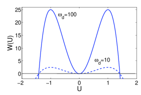
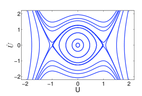
Figure 1: (a) The quartic on-site potential (1.6) for $\beta=1$ and two different values of $\omega_{d}$ ($\omega_{d}^{2}=10$ and $\omega_{d}^{2}=100$). (b) The phase plane for the single repulsive Duffing equation $\ddot{U}+\omega_{d}^{2}U-\omega_{d}^{2}\beta U^{3}=0$ for $\beta=1$ and $\omega_{d}^{2}=3.2$. Blow-up occurs only for initial positions outside the potential well (i.e., for all orbits beyond the heteroclinic orbit that is connecting the two saddles).

The repulsive $\phi^{4}$-potential (1.6), illustrated in Fig. 1(a), has a stable minimum at $U_{\mathrm{min}}=0$, corresponding to the rest energy $E_{\mathrm{min}}=W(0)=0$, and two unstable maxima located at $U^{\mp}_{\mathrm{max}}=\mp\frac{1}{\sqrt{\beta}}$, corresponding to $E_{\mathrm{max}}=W\left(\mp\frac{1}{\sqrt{\beta}}\right)=\frac{\omega_{d}^{2}}{4\beta}$.

System (1.3) shares similar phenomenological properties with those of simplified models for DNA dynamics Peyrard1 ; Peyrard2 ; Juan . To be more specific, the prototypical similarities are the following. The case $\beta>0$ is the physically relevant case for the study of energy-localization mechanisms in hydrogen-bonded crystals or DNA molecules, since in this type of models the potentials soften for large amplitudes KP92 . In particular, the potential (1.6) (which is also known as “soft quartic potential”) may correspond to the hydrogen-bridge bond between nucleotides. As it is typical in the modeling of chemical bonds (Peyrard2, , Section 2.1, pg. 269), (1.6) represents qualitatively a potential with a hard repulsive part and a softer attractive part, and it diverges as $U\rightarrow\infty$. The region $[U^{-}_{\mathrm{max}},U^{+}_{\mathrm{max}}]$, which corresponds to the potential well of depth $E_{\mathrm{max}}$, describes the region of amplitudes below the breaking of the chemical bonds.

Here, the escape problem can simply be described as escaping from the potential well (towards infinite values of the field) by crossing the saddle points $U^{\mp}_{\mathrm{max}}$ in the configuration space. In order to have escape of particles over the energy barrier $E_{\mathrm{max}}$ to the region $U>U_{\max}$, a sufficient amount of energy has to be supplied. Regarding the large-time behavior of solutions, the escape leads to blow-up of solutions in finite time.

Structure of the presentation and main findings.

The paper organization and the main results can be described as follows. Our aim is to progressively examine the potential blow-up of initial conditions involving more oscillators.

First, in Section II, we study the collapse problem for the Hamiltonian system ($\gamma=0$), i.e., the formation of finite time singularities, and find the following.

• Since the system can be seen to belong in the class of second-order evolution equations of divergent structure, it can be naturally treated, with respect to global non-existence, by the energy-type methods of GP . In particular, using differential and algebraic inequalities we derive conditions under which suitable norms (such as the $\ell^{2}$ norm) will diverge in finite time.

• Focusing on initial conditions of a single excited unit, with the other units initially located at the minimum $U_{\mathrm{min}}=0$, we derive an analytical value for the initial position of the single unit outside the potential well, which serves as a sufficient condition (threshold) for global non-existence. This value depends strongly on the parameter $\omega_{d}^{2}$ controlling the interplay of discreteness and nonlinearity. Our numerical simulations demonstrate that, indeed, blow up occurs when the analytical prediction is satisfied and a concerted escape may follow when we are in a regime where the coupling effect is significant. This is the “drive over” phenomenon, where a particular oscillator drives its neighbors over the collapse barrier. A reverse phenomenon that we also identify numerically and explore herein is the “pull back” effect, where the attraction of an initially escaped unit by the neighbors back to the stability domain, leads to solutions which exist globally in time.

• A detailed numerical analysis of the single excited site initial data reveals the existence of a “true” threshold for the position of the excited unit outside of the well, which acts as a separatrix for the above two different dynamical behaviors. For this threshold, the $\omega_{d}^{2}$-dependent analytical prediction that we analytically identify (for collapse) serves as an upper bound; the relevant comparison of the analytical and true (numerically obtained) threshold is analyzed in the different limits of the discreteness parameter.

• We also examine the global existence result of (GP, , Lemma 2.1, pg. 455) in view of the Hamiltonian system (1.3) ($\gamma=0$). We find the following: assuming negative initial time derivative of the $\ell^{2}$ norm along with a non-positive initial Hamiltonian energy fails to ensure global existence. The numerical results seem to fully support this concern.

Next, Section III deals with the collapse problem for the linearly damped system (1.3) for $\gamma>0$. Using the abstract energy methods developed in Ref. PS98 (having the advantage that they take into account the geometry of the potential energy), we find the following.

• We derive a $\gamma$-independent prediction for the position threshold outside the potential well for the single excited unit. The numerical experiments of section III.1 verify the relevance of this criterion and that, even for significantly large values of $\gamma>0$, the induced friction does not modify the scenarios found in the conservative case. In particular, friction does not affect the “pull back” effect by increasing the threshold value (as might intuitively be expected).

• The $\gamma$-independence of the threshold criterion, illustrates that only the strength of the binding forces are responsible for the “pull back” or “drive over” effects. To this end, the criterion is also applied successfully to the case where $\gamma=0$, yielding an alternative and improved upper bound to the threshold for collapse or stability. This is also corroborated by our numerical simulations.

In Section IV, we continue our analysis by studying the escape dynamics for multi-site excitations of the Hamiltonian system ($\gamma=0$). Here, we extend our arguments for a single-site excitation to the case of a few and ultimately to many site excitations, but this time, positioned inside the potential well. Our results in this setting are as follows.

• We derive an analytical threshold for collapse based on the initial “energy” of a short-length lattice-segment, depending on the discreteness parameter $\omega_{d}^{2}$. The numerical results (based on a three excited units initial configuration) validate the theoretical expectations. The threshold separates the remaining of the segment in the potential well from its escape which, in turn, is leading to collapse.

• Combining a violation of a small initial data global existence result (which can be proved by implementing the methods of Ref. cazh ), with the modulational instability analysis (based on the discrete nonlinear Schrödinger (DNLS) approximation KP92 ), we reveal the existence of three different regimes for the amplitude of a plane wave initial configuration, distinguishing between the following dynamical behaviors: modulational stability, modulational instability without escape and finally to modulational instability combined with escape. We also examine how the violation of a small data global existence criterion connects to the numerical amplitude value beyond which modulational instability leads to escape.

• For the linearly damped DKG chain, we perform numerical simulations which reveal a transient modulation instability regime for small values of damping. Nevertheless, the instability is completely suppressed eventually, in accordance with the predictions of the damped DNLS approximation.

Finally, Section V offers a discussion and a summary of our results. The complementary appendices section contains the proofs of the global nonexistence and global existence results which have been used in this paper for the analysis of the escape dynamics.

Notation.

We shall use when convenient, the short-hand notation $\{U_{n}(t)\}_{n\in\mathbb{Z}}=U(t)\in\ell^{2}$, $\{U_{n}(0)\}_{n\in\mathbb{Z}}=U(0)\in\ell^{2}$ and $\{\dot{U}_{n}(0)\}_{n\in\mathbb{Z}}=\dot{U}(0)\in\ell^{2}$, for the solution for $t>0$ and the initial conditions at $t=0$ respectively. In this notation, $\Delta_{2}$ stands for the one-dimensional discrete Laplacian

$$\left\{\Delta_{2}U\right\}_{n\in\mathbb{Z}}=U_{n+1}-2U_{n}+U_{n-1},$$

defined on $\ell^{2}$. We shall also denote by

$$(U,Y)_{\ell^{2}}=\sum_{n=-\infty}^{+\infty}U_{n}Y_{n},\;\;||U||^{2}_{\ell^{2}}=\sum_{n=-\infty}^{+\infty}U_{n}^{2},$$

the squared-$\ell^{2}$ inner product and norm respectively.

II The case of the Hamiltonian system

We may start discussing the conditions for the existence of finite-time singularities, and their relevance to the problem of escape dynamics. To this end, we have reviewed and implement in the discrete case the method of Ref. GP , on the derivation of a differential inequality for the norm $x(t):=||U(t)||_{\ell^{2}}^{2}$, and verify that it blows-up in finite time under appropriate sign conditions on the initial Hamiltonian and the time derivative of the norm.

Theorem II.1

We assume that the initial data (1.4) for the system (1.3) are such that $\mathcal{H}(0)\leq 0$ and $(U(0),\dot{U}(0))_{\ell^{2}}>0$. Then $T_{\mathrm{max}}<\infty$. More precisely, the solution blows up (in the sense that $||U(t)||^{2}_{\ell^{2}}$ becomes unbounded) on the finite interval $(0,T_{\mathrm{b}})$, with

$$T_{\mathrm{b}}=2\frac{||U(0)||^{2}}{(U(0),\dot{U}(0))_{\ell^{2}}},\;\;\mbox{and}\;\;T_{\mathrm{max}}\leq T_{\mathrm{b}}.$$ (2.1)

Proof: See Appendix A.  $\Box$

II.1 Numerical Study 1: Connection of the results of Theorem II.1 with escape dynamics

Initiating here our numerical studies, we intend to discuss the possible connections of Theorem II.1 with the problem of escape dynamics. The numerical studies will consider the system (1.3) in a form involving the variable discretization parameter $\epsilon>0$, namely:

$$\ddot{U}_{n}-\epsilon(U_{n+1}-2U_{n}+U_{n-1})+\omega^{2}_{d}(U_{n}-\beta U_{n}^{3})=0,\;\;\beta>0,\;\;\epsilon=\frac{1}{h^{2}},$$ (2.2)

on the interval $\left[-L,L\right]$, supplemented with Dirichlet boundary conditions. The solution of (2.2) is described by the vector $U\in\mathbb{R}^{K+2}$

$$U(t)=\left(U_{0}(t),U_{1}(t),\ldots U_{K+1}(t)\right),\;\;U_{0}(t)=U_{K+1}(t)=0,$$ (2.3)

where $U_{n}(t):=U(x_{n},t)$, $x_{n}=-\frac{L}{2}+nh$, $n=0,\ldots,K+1$, for all $t\geq 0$. With the change of variable $t\rightarrow\frac{1}{h}t$, we rewrite the initial-boundary value problem for (2.2) in the form

$$\ddot{U}_{n}-(U_{n+1}-2U_{n}+U_{n-1}) + \Omega_{d}^{2}(U_{n}-\beta U_{n}^{3})=0,\;t>0\;\;n=1,\ldots,K,\;\;\Omega_{d}^{2}=h^{2}\omega_{d}^{2},$$ (2.6)

$$U(0),\;\dot{U}(0)\in\mathbb{R}^{K+2},$$

$$U_{0}=U_{K+1}=0,\;\;t\geq 0.$$

Our rescaling of the lattice parameter out of the problem makes it important that we add here a comment about the nature of the continuous and the so-called anti-continuous limit. In the latter, we need to consider within Eq. (1.3) the limit of $\omega_{d}^{2}\rightarrow\infty$. There, the nonlinearity dominates, and we are essentially in the regime of individual (uncoupled) oscillators. On the other hand, for small values of $\omega_{d}^{2}$, the linear coupling term becomes important. However, due to the nature of our model, we are reaching the asymptotically linear limit (rather than the continuum limit) as $\omega_{d}^{2}\rightarrow 0$.

We will perform numerical simulations for the simplest case of initial data

$$U_{n}(0) = A\delta_{n,0},$$ (2.7)

$$\dot{U}_{n}(0) = B\delta_{n,0},$$ (2.8)

where $\delta_{n,0}=1$ at site $n=0$ and zero elsewhere (Kronecker $\delta$), for $A,B\in\mathbb{R}$. For the initial data (2.7)-(2.8), the condition for the initial Hamiltonian $\mathcal{H}(0)\leq 0$ reads:

$$\frac{B^{2}}{2}+\left(1+\frac{\Omega_{d}^{2}}{2}\right)A^{2}\leq\frac{\beta\Omega_{d}^{2}}{4}A^{4},\;\;\Omega_{d}^{2}=h^{2}\omega_{d}^{2}.$$ (2.9)

Then, it can readily be observed that the quartic equation

$$\frac{\beta\Omega_{d}^{2}}{4}A^{4}-\left(1+\frac{\Omega_{d}^{2}}{2}\right)A^{2}-\frac{B^{2}}{2}=0,$$ (2.10)

possesses the unique positive root (for $A^{2}$):

$$A^{2}_{*}=2\left[\frac{\left(1+\frac{\Omega_{d}^{2}}{2}\right)}{\beta\Omega_{d}^{2}}+\sqrt{\frac{\left(1+\frac{\Omega_{d}^{2}}{2}\right)^{2}}{\beta^{2}\Omega_{d}^{4}}+\frac{B^{2}}{2\beta\Omega_{d}^{2}}}\right],\;\;\Omega_{d}^{2}=h^{2}\omega_{d}^{2}.$$ (2.11)

Therefore, for the initial data (2.7)-(2.8), the condition (2.9) is satisfied if

$$A<-{A_{*}}\;\;\mbox{or}\;\;A>{A_{*}}.$$ (2.12)

It can be easily checked from (2.11) that

$$-A_{*}<U^{-}_{\mathrm{max}}=-\frac{1}{\sqrt{\beta}}\;\;\mbox{and}\;\;A_{*}>U^{+}_{\mathrm{max}}=\frac{1}{\sqrt{\beta}},\;\;\mbox{for all}\;\;\omega_{d}^{2},h,\beta>0,$$

recalling that $U^{\mp}_{\mathrm{max}}$ denote the location of the saddle points of the on-site potential. The condition on the sign of the time derivative of the $\ell^{2}$ norm for the initial data (2.7)-(2.8) reads

$$(U_{n}(0),\dot{U}_{n}(0))_{\ell^{2}}=AB>0.$$ (2.13)

First, we remark that condition (2.12) is not directly related to the core question of escape dynamics, which is the escape from the potential-well of the on-site potential for initial configurations of the chain inside the well: assuming initially only one excited unit, the conditions of Theorem II.1 imply that the initial position of this unit should be located outside the interval $(U^{-}_{\mathrm{max}},U^{+}_{\mathrm{max}})$ defining the well.

On the other hand, exciting initially only one unit outside the well, with all the others located at the minimum $U_{\mathrm{min}}=0$, is indeed of strong physical relevance in connection to another central question regarding the escape dynamics (Dirk1, , pg. 041110-4): does this initially escaped unit continue its excursion beyond the saddle-point barrier or can it, in fact, be pulled back into the bound chain configuration $U_{n}\in(U^{-}_{\mathrm{max}},U^{+}_{\mathrm{max}})$ by the restoring binding forces exerted by the neighbors? Alternatively, can the unit which is initially located outside the well, drag neighboring ones closer to or, in a more extreme scenario, over the barrier? The answer to these important questions should critically depend on the strength of the interactions between the oscillating units, imposed by the linear coupling.

In view of the above questions, the conditions (2.12)-(2.13) seem to be quite relevant, in the sense that they determine the behavior of the whole chain regarding the escape dynamics if the analytical threshold (2.12) is crossed by at least one unit: in the anti-continuum limit $\epsilon\rightarrow 0$ [or $\Omega_{d}^{2}\rightarrow\infty$ since, from our scaling $\Omega_{d}^{2}=O\left(\frac{1}{\epsilon}\right)=O(h^{2})$], according to Theorem II.1, we expect that the initially escaped unit will continue its motion beyond the saddle-point barrier, while the other units should remain in the well. This is because in this case, the escaped unit is not interacting with the other units of the chain. The fact that $||U(t)||_{\ell^{2}}$ approaches infinity at finite time is due to the unboundedness of the energy of this unit in finite time; while the other units remain in the well, the excursion of the escaped unit implies actually the unboundedness of the $\mathrm{sup}$-norm $||U(t)||_{\infty}=\sup_{n\in\mathbb{Z}}|U_{n}(t)|$ in finite time and, in turn, the unboundedness of the $||U(t)||_{\ell^{2}}$-energy due to the inequality:

$$||U(t)||_{\infty}\leq||U(t)||_{\ell^{2}}.$$ (2.14)

Note that in the infinite lattice only this side of the inequality holds in contrast with the finite lattice, where the equivalence of norms

$$||U(t)||_{\infty}\leq||U(t)||_{\ell^{2}}\leq\sqrt{N}||U(t)||_{\infty},$$ (2.15)

is valid in the $N$-dimensional space.

In the discrete regime $\epsilon=O(1)$ (i.e., for moderate values of $\Omega_{d}^{2}$, as e.g., $\Omega_{d}^{2}=10$ used in Ref. Peyrard ) and in the continuum limit $\epsilon\rightarrow\infty$, it is expected from Theorem II.1 and (2.14) that a concerted escape of the whole chain will take place, while the time of escape of the whole chain should depend on the coupling strength.

The above analytical expectations and questions have been tested for $\beta=1$, $h=0.5$ and varying the parameter $\omega_{d}^{2}$. The initial speed is taken to be $B=0.001$, i.e., a small initial velocity of the one-excited unit is provided in order to satisfy the condition (2.13).

The first observation of the numerical studies is the justification of (2.12)-(2.13) as sufficient conditions for blow-up and for the continuation of the excursion of the one-excited unit beyond the saddle point barrier when $A>A_{*}$.

The second question examined numerically, concerns the dynamics of the chain when the one-excited unit is located in the region $1<A<A_{*}$, i.e., beyond the location of the saddle point, but below the analytical critical value $A_{*}$. There, our numerical simulations revealed that blow-up occurs for initial positions of the unit $A<A_{*}$; hence, conditions (2.12)-(2.13), although sufficient, are not strictly necessary for blow-up, which was found to occur for the one-excited unit even when its location is below the analytical value $A_{*}$.

However, and more importantly, the numerical studies revealed the existence of a new barrier (threshold) $\mathcal{U}_{\mathrm{thresh}}$, located beyond the position of the saddle point $U^{+}_{\mathrm{max}}=1$, with an important dynamical property. Although $U^{+}_{\mathrm{max}}<\mathcal{U}_{\mathrm{thresh}}$, when the excited unit is initially located at position $A$ satisfying $U^{+}_{\mathrm{max}}<A<\mathcal{U}_{\mathrm{thresh}}\leq A_{*}$, it may be pulled back to the potential well and the solution exists globally. As mentioned above, the position of the barrier $\mathcal{U}_{\mathrm{thresh}}$, satisfying $U^{+}_{\mathrm{max}}<\mathcal{U}_{\mathrm{thresh}}\leq A_{*}$, is determined by the restoring binding forces. This fact is demonstrated in Fig. 2(a), showing the evolution of the chain in strong coupling regime ($\Omega_{d}^{2}=1$). A single-excited unit, of initial amplitude $A=1.2$ (satisfying $U^{+}_{\mathrm{max}}=1<A<A_{*}$), is being pulled back inside the well, due to the sufficiently strong coupling with its neighbor units. This verifies our analytical prediction, that restoring forces (depending on the discreteness) can prevent the escape of elements of the chain initialized outside the potential well. This is what we will refer to as the “pull back” effect. After this effect takes place for the single-excited unit and it gets “retracted” inside the potential well $(U^{-}_{\mathrm{max}},U^{+}_{\mathrm{max}})$, the whole chain performs globally existing wave motions.

The fact that blow-up occurs for $A>A_{*}=2.44$, as well as the result of Fig. 2(a), confirm the existence of the threshold $\mathcal{U}_{\mathrm{thresh}}$ and motivate a further numerical investigation to determine its exact location. The corresponding numerical value is found to be $\mathcal{U}_{\mathrm{thresh}}\sim 1.8<A_{*}$ for the near-continuum case ($\Omega_{d}^{2}=1$). Concluding, we have shown that:

1. blow-up occurs when $A>\mathcal{U}_{\mathrm{thresh}}$;

2. a single-excited unit is pulled back to the potential well when $U^{+}_{\mathrm{max}}\leq A\leq\mathcal{U}_{\mathrm{thresh}}$;

3. finally and in connection to our analytical result, $A_{*}$ provides an upper bound for the exact value of $\mathcal{U}_{\mathrm{thresh}}\in(U^{+}_{\mathrm{max}},A_{*})$ and blow-up always takes place, as predicted for $A>A_{*}$.

Figure 2: (a) Evolution of a single-excited unit initially located at $A=1.2$, satisfying $U^{+}_{\mathrm{max}}=1<A<A_{*}=2.45$; the value of $U^{+}_{\mathrm{max}}$ is indicated by the dashed (red) line. Although the unit is initially beyond the saddle point (but below both the numerical threshold $\mathcal{U}_{\mathrm{thresh}}\sim 1.8$ and the analytical value $A_{*}$), it is pulled back in the potential well, leading to globally existing dynamics. Lattice parameters are $\beta=1$, $\Omega_{d}^{2}=1$, for $h=0.5$ and $\omega_{d}^{2}=4$. (b) In this case, the single-excited unit, initially at $A=2$, is pulling the adjacent neighbors towards escape from the potential well. Here, $A_{*}=4.24$ and $\mathcal{U}_{\mathrm{thresh}}\sim 1.9$. The lattice parameters are: $\beta=1$, $\Omega_{d}^{2}=0.25$, for $h=0.5$ and $\omega_{d}^{2}=1$.

The dependence of the analytical blow-up threshold prediction $A_{*}$ on the discreteness parameter $\omega_{d}^{2}$ (for fixed values of $\beta=1$ and $h=0.5$), is depicted by the solid (black) line in Fig. 3. The respective plot for the numerically obtained value, $\mathcal{U}_{\mathrm{thresh}}$ is also depicted –in the same plot– by (red) circles. Comparing the two results, we conclude that $A_{*}$ tends to be more accurate as an upper bound for the “real” barrier $U_{\mathrm{thresh}}$, for small to moderate values of $\omega_{d}^{2}$. On the other hand, a constant –but reasonable– discrepancy between the analytical and the numerical value is found in the intermediate regime between moderate and large values of $\omega_{d}^{2}$ (the latter corresponding to the near anti-continuum regime of essentially uncoupled nonlinear sites). This discrepancy can be explained as follows: approaching the anti-continuum limit as $\omega_{d}^{2}\rightarrow\infty$, it is naturally expected that the threshold value $\mathcal{U}_{\mathrm{thresh}}\rightarrow U^{+}_{\mathrm{max}}=\frac{1}{\sqrt{\beta}}$ since, due to the increasingly weaker interactions between the oscillating units, the system (2.2) is asymptotically reduced to a single repulsive Duffing equation for the single-excited unit –see Fig. 1(b). On the other hand, it follows from (2.11) that $A_{*}\rightarrow\frac{\sqrt{2}}{\sqrt{\beta}}$ as $\omega_{d}^{2}\rightarrow\infty$. Thus, a constant difference between the threshold values is found in this regime, namely $A_{*}-\mathcal{U}_{\mathrm{thresh}}\sim\frac{\sqrt{2}-1}{\sqrt{\beta}}$ (for large values of $\omega_{d}^{2}$), which is observed in Fig. 3.

In the asymptotically linear limit of $\omega_{d}^{2}\rightarrow 0\;(\Omega_{d}^{2}\rightarrow 0)$, Eq. (2.11) predicts that $A^{*}\rightarrow\infty$. This prediction can also be justified, given the absence (in that limit) of the nonlinearity that is responsible for the blow-up. In the corresponding limit, we observe numerically that $\mathcal{U}_{\mathrm{thresh}}\rightarrow\infty$, in accordance with the analytical prediction $A_{*}\rightarrow\infty$. The limits $A_{*},\,\mathcal{U}_{\mathrm{thresh}}\rightarrow\infty$ as $\omega_{d}^{2}\rightarrow 0$ are shown in Fig. 3.

Furthermore, as the above limit is approached and due to the increasingly more significant role of the interactions between the units, if the excited amplitude has crossed the barrier $\mathcal{U}_{\mathrm{thresh}}$ for blow-up, it will enforce the other units to escape from the potential well. This is “drive over” the barrier scenario, clearly demonstrated in Fig. 2(b), which shows the evolution of the chain for lattice parameters $\Omega_{d}^{2}=0.25$, i.e., $\omega_{d}^{2}=1$ for $h=0.5$. The single-excited unit with an initial amplitude $\mathcal{U}_{\mathrm{thresh}}\sim 1.9<A=2<A_{*}$, pulls the adjacent neighbors, enabling them to cross the saddle point towards escape from the potential well.

The accuracy of the analytical prediction for the escape threshold will be improved in the next section dealing with the linearly damped version of (1.3). The improvement, also depicted in Fig. 3 with the dashed (blue) line will be discussed there, in detail.

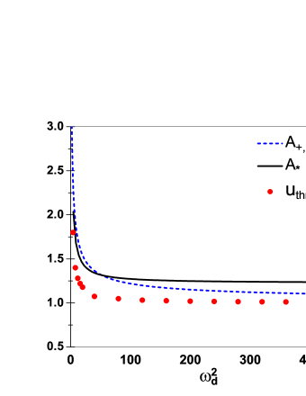
Figure 3: Theoretical predictions for the blow-up amplitude for a single site excitation, as a function of $\omega_{d}^{2}$, compared to the actual numerical value $\mathcal{U}_{\mathrm{thresh}}$. The solid (black) curve corresponds to the analytical upper bound $A_{*}$ [cf. Eq. (2.11)] and the dashed (blue) curve to the analytical value $A_{+,*}$ [cf. Eq. (3.12)]. Bullets (in red) denote the numerical values $\mathcal{U}_{\mathrm{thresh}}$. An asymptotic discrepancy appears for $A_{*}$ as $\omega_{d}^{2}\rightarrow\infty$ while the accuracy of $A_{+,*}$ increases as the anti-continuum limit of uncoupled sites is approached– see discussion in the text. The parameter values are: $h=0.5$, $\beta=1$.

II.2 Discussion on the sign-condition (2.13).

We conclude this section with a discussion of (GP, , Lemma 2.1, pg. 455) for the lattice dynamical system (1.3)-(1.4). According to the abstract results of Ref. GP , keeping the condition $\mathcal{H}(0)\leq 0$ and violating the sign condition $(U(0),\dot{U}(0))_{\ell^{2}}>0$ should lead to global existence. In terms of the initial data (2.7)-(2.8), the result (GP, , Lemma 2.1, pg. 455) implies that the initially escaped unit will be pulled back and return to the potential well. For example, under the assumption

$$\dot{x}(0)=2(U(0),\dot{U}(0))_{\ell^{2}}<0,$$ (2.16)

we will reconsider the differential inequality (5.18) in the form

$$\frac{\ddot{x}(t)}{[\dot{x}(t)]^{2}}\geq\frac{3}{2x(t)}.$$ (2.17)

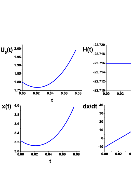
Figure 4: Time evolution of the amplitude $U_{0}$, Hamiltonian $\mathcal{H}$ (denoted by $H(t)$ in the figure), norm $x$ and time derivative of the norm $dx/dt$ for a single-excited unit with initial data (2.7)-(2.8) with $A=1.8$ and $B=-5.5$; the lattice parameters are $\Omega_{d}^{2}=10$ ($\omega_{d}^{2}=40$, $h=0.5$), $\beta=1$, corresponding to a highly nonlinear discrete regime. The top left panel shows the excursion to infinity for the one-excited unit; the top right panel depicts the negative (constant) Hamiltonian $\mathcal{H}(t)=\mathcal{H}(0)\sim 22.7$; the bottom left panel shows the change of the slope of the norm $x(t)$ and its increase to infinity after time $t^{*}$; the bottom right panel depicts the change of sign of $\dot{x}(t)$ after time $t^{*}$.

Integrating (2.17) in the interval $[0,t]$ for arbitrary $t\in[0,T]$, the interval of existence, we find that

$$-\frac{1}{\dot{x}(t)}+\frac{1}{\dot{x}(0)}\geq\frac{3}{2}\int_{0}^{t}\frac{1}{x(s)}ds,$$

which can be rewritten as

$$\frac{1}{\dot{x}(t)}\leq\frac{1}{\dot{x}(0)}-\frac{3}{2}\int_{0}^{t}\frac{1}{x(s)}ds.$$ (2.18)

Then, the assumption $\dot{x}(0)=2(U(0),\dot{U}(0))<0$, as well as the positivity of the norm function $x(t)=||U(t)||^{2}_{\ell^{2}}\geq 0$ for all $t\in[0,T]$ in the interval of existence $[0,T]$ should imply that $\frac{1}{\dot{x}(t)}\leq 0$, i.e.,

$$\dot{x}(t)\leq 0,\;\;\mbox{{\emph{for all}}}\;\;t\in[0,T].$$ (2.19)

Integrating (2.18) once more in $[0,T]$, we see that

$$x(t)\leq x(0),\;\;\mbox{for all}\;\;t\in[0,T].$$ (2.20)

Letting $t\rightarrow\infty$ in (2.20) implies that $T_{\mathrm{max}}=\infty$ and

$$\limsup_{t\rightarrow\infty}||U(t)||^{2}_{\ell^{2}}\leq||U(0)||_{\ell^{2}}^{2}.$$ (2.21)

Hence, the solution $U(t)=\left\{U_{n}(t)\right\}_{n\in\mathbb{Z}}$ should be defined in $[0,\infty)$ and be uniformly bounded.

However, the validity of (2.18) for all $t\in[0,T]$ –the interval of existence– should be put under question: Although the continuity of $\dot{x}(t)=2(U(t),\dot{U}(t))_{\ell^{2}}<0$ in $[0,T]$, the assumption $\dot{x}(0)=2(U(0),\dot{U}(0))_{\ell^{2}}<0$ and (2.18) guarantee the existence of $t_{1}>0$, such that $\dot{x}(t)\leq 0$ for all $t\in[0,t_{1}]$, this assumption and (2.18) do not guarantee that $t_{1}=T$. Recall that the inequality (5.14) implies that $\ddot{x}(t)>0$ for all $t\in[0,T]$, hence the function $\dot{x}(t)$ is increasing in the interval $[0,T]$. Due to this fact, the existence of a $t_{2}>t_{1}>0$, such that $\dot{x}(t)>0$ for all $t\in[t_{2},T]$, cannot be excluded.

Our concerns on the arguments of (GP, , Lemma 2.1, pg. 455) have been tested numerically for the initial data (2.7)-(2.8). If the above arguments were valid, the condition $\mathcal{H}(0)\leq 0$ on the initial Hamiltonian implying (2.12) on the position $A$ of the single-excited unit, together with (2.16) which for the initial data (2.7)-(2.8) reads as

$$(U(0),\dot{U}(0))_{\ell^{2}}=AB<0,$$ (2.22)

should imply the pull-back of the initially escaped unit inside the potential well $(U^{-}_{\mathrm{max}},U^{+}_{\mathrm{max}})$.

In Fig. 4, we present the results obtained, after numerically integrating Eq. (1.3), with initial conditions of the form of Eqs. (2.7)-(2.8), with $A=1.8$ and $B=-5.5$, thus satisfying (2.12), and the condition (2.22), since $(U(0),\dot{U}(0))_{\ell^{2}}=AB=-9.9<0$. The lattice parameters are $\Omega_{d}^{2}=10$ ($\omega_{d}^{2}=40$ and $h=0.5$), $\beta=1$, while the initial Hamiltonian is negative $\mathcal{H}(0)=-22.7$ as required, and remains negative and constant in the interval of existence, due to conservation of energy, as shown in top right panel of Fig. 4. In the bottom right panel of Fig. 4, we show the time evolution of the function $\dot{x}(t)=2(U(t),\dot{U}(t))_{\ell^{2}}$. The initial value of $\dot{x}(t)$ is negative, as required by (GP, , Lemma 2.1, pg. 455), and remains negative up to some finite time, say $t^{*}$. On the other hand, at $t=t^{*}$ (where $\dot{x}(t^{*})=0$), the function $\dot{x}(t)$ becomes positive, and remains positive for all $t>t^{*}$, justifying the contradiction with the arguments of Ref. GP for global existence. Also, since $\ddot{x}(t)>0$ for all $t\in[0,T]$, $\dot{x}(t)$ is strictly increasing, and the norm $x(t)$ is concave up for all $t\in[0,T]$, as shown in bottom left panel of Fig. 4. Choosing a time $t_{2}>t^{*}$ for which $\dot{x}(t)>0$ for all $t\geq t_{2}>t^{*}>0$, the results of Theorem II.1 come into play again: since the system (1.3)-(1.4) is autonomous, using the time $t_{2}$ as an initial time, and $(U(t_{2}),\dot{U}(t_{2}))_{\ell^{2}}$ as initial data, we may repeat the arguments of Theorem II.1 establishing that the initially escaped unit can never return in the bound-chain configuration, as observed in the top left panel of Fig. 4.

III The case of the linearly damped system

In this section, we will consider the conditions for collapse in the case of the linearly damped analogue of Eq. (1.3), namely,

$$\ddot{U}_{n}+\gamma\dot{U}_{n}-(U_{n+1}-2U_{n}+U_{n-1})+\omega^{2}_{d}(U_{n}-\beta U_{n}^{3})=0,\;\;\;\gamma>0,\;\;\beta>0,$$ (3.1)

with the initial conditions:

$$U_{n}(0)\;\;\mbox{and}\;\;\dot{U}_{n}(0)\in\ell^{2}.$$ (3.2)

In the damped system (3.1), we may consider the abstract methods of Ref. PS98 and prove global non-existence by replacing the sign condition on $\mathcal{H}(0)$ with an appropriate smallness condition. Added to the assumption of the possibly positive Hamiltonian, a condition for a sufficiently large initial size of the quartic term of the Hamiltonian is derived, replacing the one –imposed in the Hamiltonian case– concerning the sign of the time derivative of the norm of the initial data. Of primary interest here, will be the discussion of the effect of the damping in the behavior of the whole chain, regarding its single node or possibly concerted escape from the potential well.

The global non-existence result of the section is stated as follows.

Theorem III.1

We assume that the initial Hamiltonian satisfies

$$\mathcal{H}(0)<\frac{\omega_{d}^{2}}{4\beta},$$ (3.3)

and that, initially, the quartic term is sufficiently large, in the sense that the $\ell^{4}$-norm of the initial position satisfies:

$$||U(0)||_{\ell^{4}}=\left(\sum_{n=-\infty}^{+\infty}U_{n}(0)^{4}\right)^{\frac{1}{4}}>\frac{1}{\sqrt{\beta}}.$$ (3.4)

Then, the solution of (3.1)-(3.2) does not exist globally in time.

Proof:. See Appendix B.   $\Box$

III.1 Numerical Study 2: Connection of the results of Theorem III.1 with escape dynamics

As in section II.1, in the numerical simulations we will consider the linearly damped version of (2.2) involving the linear coupling parameter $\epsilon>0$

$$\ddot{U}_{n}+\gamma\dot{U}_{n}-\epsilon(U_{n+1}-2U_{n}+U_{n-1})+\omega^{2}_{d}(U_{n}-\beta U_{n}^{3})=0,\;\;\beta>0,\;\;\gamma>0,\;\;\epsilon=\frac{1}{h^{2}},$$ (3.5)

on the interval $\left[-L,L\right]$, supplemented with Dirichlet boundary conditions. The initial-boundary value problem for the damped system (3.5) can be written with the change of variable $t\rightarrow\frac{1}{h}t$ as

$$\ddot{U}_{n}+\gamma h\dot{U}_{n}-(U_{n+1}-2U_{n}+U_{n-1}) + \Omega_{d}^{2}(U_{n}-\beta U_{n}^{3})=0,\;t>0\;\;n=1,\ldots,K,\;\;\Omega_{d}^{2}=h^{2}\omega_{d}^{2},$$ (3.8)

$$U(0),\;\dot{U}(0)\in\mathbb{R}^{K+2},$$

$$U_{0}=U_{K+1}=0,\;\;t\geq 0.$$

In the numerical simulations we will again consider the single-unit initial excitation (2.7)-(2.8). For the initial data (2.7)-(2.8), conditions (3.3)-(3.4) are implemented as:

$$\frac{B^{2}}{2}+\left(1+\frac{\Omega_{d}^{2}}{2}\right)A^{2}-\frac{\beta\Omega_{d}^{2}}{4}A^{4}<\frac{\Omega_{d}^{2}}{4\beta},\;\;\mbox{and}$$ (3.9)

$$A>\frac{1}{\sqrt{\beta}}.$$ (3.10)

Here, the quartic equation

$$\frac{\beta\Omega_{d}^{2}}{4}A^{4}-\left(1+\frac{\Omega_{d}^{2}}{2}\right)A^{2}-\frac{B^{2}}{2}+\frac{\Omega_{d}^{2}}{4\beta}=0,$$ (3.11)

has in terms of $A^{2}$ the two roots:

$$A^{2}_{\pm,*}=2\left[\frac{\left(1+\frac{\Omega_{d}^{2}}{2}\right)}{\beta\Omega_{d}^{2}}\pm\sqrt{\frac{\left(1+\frac{\Omega_{d}^{2}}{2}\right)^{2}}{\beta^{2}\Omega_{d}^{4}}+\frac{B^{2}}{2\beta\Omega_{d}^{2}}-\frac{1}{4\beta^{2}}}\right],\;\;\Omega_{d}^{2}=h^{2}\omega_{d}^{2}.$$ (3.12)

Note that $A^{2}_{+,*}>0$, $A^{2}_{+,*}>A^{2}_{-,*}$ and $A^{2}_{-,*}>0$ if and only if $B\in\left(-\frac{\Omega_{d}}{\sqrt{2\beta}},\frac{\Omega_{d}}{\sqrt{2\beta}}\right)$. Furthermore, it can be seen that

$$A^{2}_{+,*}>\frac{1}{\beta},\;\;\;\;\mbox{for all}\;\;\omega_{d}^{2},h,\beta>0.$$ (3.13)

Then, both conditions (3.9) and (3.10) are satisfied, as required, if

$$A<-A_{+,*}\;\;\mbox{or}\;\;A>A_{+,*}.$$ (3.14)

As in the Hamiltonian case, conditions (3.14) imply that the initial position of the excited unit should be located outside the interval $(U^{-}_{\mathrm{max}},U^{+}_{\mathrm{max}})$ defining the well, due to (3.13). We point out that this condition of blow-up bears no signature of the damping parameter $\gamma$ and, hence, can be used for the Hamiltonian case as well, a point evident in Fig. 3 and one to which we return below.

However, the question of whether the single-unit, initially placed outside the saddle-point barrier, will escape or whether it will be pulled back into the well by its neighboring units, becomes even more interesting due to the presence of the damping: the question is if damping has an additional effect in increasing the value of the threshold between “pull back” and collapse. Since the threshold is increased as the strength of the coupling forces is increased (cf. Fig. 3), one might expect that that the same would happen with the damping force.

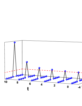
Figure 5: Evolution of the damped chain for lattice parameters $\Omega_{d}^{2}=10$ ($\omega_{d}^{2}=40$, $h=0.5$) and $\beta=1$. The central excited unit $n=0$ has initial amplitude $A=1.4$ and initial velocity $B=0$. The large damping, characterized by the parameter $\gamma=2000$, does not affect the threshold value for the “pull back” effect.

The time evolution of the damped chain, for lattice parameters $\Omega_{d}^{2}=10$ ($\omega_{d}^{2}=40$, $h=0.5$ –corresponding to a moderately discrete regime) and $\beta=1$, is shown in Fig. 5. For this set of parameters the analytical threshold for the amplitude of the single-excited unit, calculated by (3.12), is $A_{+,*}=1.36$. To test this prediction, we consider an initial amplitude of $A=1.4$ and an initial speed $B=0$ as per the Theorem III.1. In order to investigate the friction-induced effects, we consider a relatively large value of the damping parameter, i.e., $\gamma=2000$. Figure 5 shows the escape of the excited unit to infinity. On the other hand, Fig. 6(a) visualizes the rapid increase of the kinetic energy of the single unit $n=0$, despite of the fact that the total energy is dissipated according to the identity (5.25) as long as the solution exists. The evolution of the kinetic energy is also shown in Fig. 6(b), but for lattice parameters closer to the asymptotically linear regime, i.e., for $\Omega_{d}^{2}=1$ (and $\beta=1$ as well). Comparing the two panels of Fig. 6, it is evident that the initially excited unit at $n=0$ does not affect its neighboring units in the discrete case (a), in the sense that the energy remains localized at this site; on the other hand, in case (b), due to the stronger coupling, the central excited unit pulls the adjacent units at sites $n=\pm 1$ towards the saddle point, and their kinetic energy is increased compared to case (a). Numerical simulations have been also been performed for other values of $\gamma$, and they all have justified the prediction of Theorem III.1: when $A>A_{+,*}$, the collapse does not depend on the value of the damping parameter; furthermore, the true threshold $\mathcal{U}_{\mathrm{thresh}}$ is also $\gamma$-independent. Therefore, the “drive over” and “pull back” effects are chiefly controlled by the strength of the coupling forces and not from the damping. The failure of the intuitive expectation that dissipation should decay away the motion of the oscillators and hence be less conducive to collapse is evident here. This is predominantly due to the principal role of dissipation in decreasing the overall energy of the oscillator chain; yet, the latter scenario can be achieved by large amplitudes due to the nonlinearity, hence the concerted effect of energy decrease due to dissipation and its achievement by increased (squared) amplitudes due to nonlinearity gives rise to the finite time blow-up analyzed above.

Another interesting feature is the following. The analytical value $A_{+,*}$ provided by (3.12), shows an increased accuracy –in the parameter regime ranging from the moderately to the highly discrete (and the anti-continuum)– as an estimate of the numerical threshold $\mathcal{U}_{\mathrm{thresh}}$, below which the single unit will be pulled back by the exerted forces of the neighbors, and above which the chain configuration collapses. This improvement is due to the fact that the proof of Theorem III.1 takes into more detailed account the geometry of the potential energy $W(U)$. Since the proof of Theorem III.1 is independent of the damping parameter, and is also valid in the Hamiltonian case, we return to Fig. 3, where the dashed (blue) curve depicts $A_{+,*}$ as a function of $\omega_{d}^{2}$ (for fixed $B=0$, $h=0.5$ and $\beta=1$). The increased accuracy of $A_{+,*}$ [dashed (blue) line] towards the anti-continuum regime is explained directly from (3.12) since $A_{+,*}\rightarrow U^{+}_{\mathrm{max}}=\frac{1}{\sqrt{\beta}}$ as $\omega_{d}^{2}\rightarrow\infty$, and the constant discrepancy for $A_{*}$ asymptotically vanishes. Also, in the asymptotically linear case of $\omega_{d}^{2}\rightarrow 0$, $A_{+,*}\rightarrow\infty$, thus it correctly predicts the asymptotic behavior of $\mathcal{U}_{\mathrm{thresh}}$ in this limit. For moderate values of $\omega_{d}^{2}$, a comparison of (2.11) and (3.12) indicates that $A_{*}$ may be preferable to $A_{+,*}$ in this intermediate regime. Nevertheless, $A_{+,*}$ accurately captures both asymptotic limits and in the intermediate regime both $A_{*}$ and $A_{+,*}$ are expected to be least accurate due to the relevance of the terms omitted in the derived (algebraic and differential) inequalities.

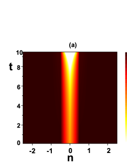
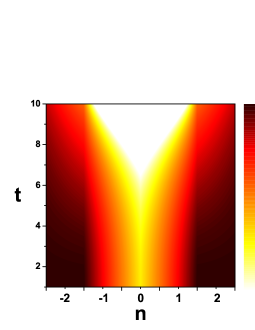
Figure 6: Contour plots showing the evolution of the kinetic energy in the damped lattice $\gamma=2000$, $\beta=1$. The central excited unit $n=0$ at initial position $A>A_{+,*}$ and velocity $B=0$. (a) $\Omega_{d}^{2}=10$ ($\omega_{d}^{2}=40$, $h=0.5$)–this is within the moderately discrete regime. (b) $\Omega_{d}^{2}=1$ ($\omega_{d}^{2}=4$, $h=0.5$)–this is in the vicinity of the asymptotically linear regime.

IV Scenarios for escape for multi-site excitations

We now move progressively away from the single site excitation scenario and toward settings where the energy of the chain becomes concentrated within a (wider than one site, yet confined) region Dirk1 . Even if initially the energy is equally shared among all units, after a certain time, the dynamics may lead to its redistribution, so that at least one of the involved units concentrates sufficient energy, to overcome the barrier defined by the saddle point of the potential. In this section, we will first consider such an escape scenario, focusing on the evolution of a small lattice segment. More specifically, we will consider the evolution of a few-site excitation, by means of the energy methods developed in the previous sections.

Then, we will study escape dynamics of the chain, induced by the modulation instability mechanism Dirk1 ; KP92 . In the latter case, the initial excitation will involve a plane wave extending throughout the chain. We shall review the conditions for modulation instability of plane waves for (2.2) and how this instability may be related to a potential escape of the modulationally unstable excitation.

Finally, deriving conditions for the global existence of initial data of sufficiently small energy, we shall investigate how the possible violation of the global existence assumptions may be connected to the escape mechanism, and formulate conditions for escape dynamics. This approach will consider solely an initial condition in the form of a plane wave.

IV.1 Energy methods on a lattice segment and escape dynamics

In view of the energy methods discussed in the previous sections and motivated by the first localization scenario discussed above, we focus on the study of the evolution of a fixed segment of the lattice. In particular, we seek appropriate conditions for the “initial energy” of this segment, which may lead to an escape process.

We consider again system (2.2) on the interval $[-L,L]$ supplemented with Dirichlet boundary conditions. Here, we will study the evolution of a lattice segment occupying the unit subinterval $\left[-\frac{1}{2},\frac{1}{2}\right]$ $\subset$ $[-L,L]$ together with the first neighbors adjacent to the points $-\frac{1}{2}$ and $\frac{1}{2}$.

The number of oscillators located outside the piece of the chain of unit length $I=\left[-\frac{1}{2},\frac{1}{2}\right]$ is

$$\theta=2\left\lceil\frac{\left(\frac{L}{2}-\frac{1}{2}\right)(K+1)}{L}\right\rceil,$$ (4.1)

where $\lceil x\rceil=\min\left\{n\in\mathbb{Z}\,|\,n\geq x\right\}$, $x\in\mathbb{R}$. Then the number of oscillators included in the unit interval $I$ is

$$m=K+2-\theta.$$ (4.2)

We distinguish between two different possibilities for the endpoints of $I$ –cf. cases $\mathrm{A}$ and $\mathrm{B}$ below.

$\mathrm{Case\leavevmode\nobreak\ A}.$ The simplest case is when the endpoints of $I$ are occupied by oscillators. In this case, the lattice spacing satisfies

$$(m+1)h=1,$$ (4.3)

and the unit interval $I$ consists of $\lambda=m+2$ oscillators, the $m$ included in $I$ together with the two endpoints.

We denote by $I^{\prime}$ the interval which comprises $I$ and the two adjacent ones. The interval $I^{\prime}$ consists of $\lambda+2=m+4$ oscillators. The length of $I^{\prime}$ is, due to (4.3),

$$L^{\prime}=1+2h=\frac{m+3}{m+1}.$$ (4.4)

We also assume that the endpoints of $I^{\prime}$ occupied by the neighbors adjacent to the endpoints of $I$, are located at the sites $k$ and $k+\lambda+1$. Then, we may decompose the solution configuration vector (2.3) as $U=U^{L\setminus I}+U^{I}$, where

$$U^{L\setminus I} = \left(U_{0},U_{1},\ldots U_{k-1},U_{k},0,\ldots,0,U_{k+\lambda+1},\ldots,U_{K+2}\right),$$ (4.5)

$$U^{I} = \left(0,\ldots,0,U_{k+1},U_{k+2},\ldots,U_{k+\lambda},0\ldots,0\right).$$ (4.6)

The initial conditions $U(0),\dot{U}(0)\in\mathbb{R}^{K+2}$ are decomposed similarly. Since the decomposition is linear, it follows from (2.2) that the elements $U^{L\setminus I}$ and $U^{I}$ satisfy, respectively, the equations:

$$\ddot{U}_{n}^{I}-\epsilon\Delta_{d}U^{I}_{n}+\omega_{d}^{2}U^{I}_{n}-\beta\omega_{d}^{2}U^{I}_{n}\leavevmode\nobreak\ U_{n}^{2}=0,\;\;n=0,\ldots,K+2,$$

$$\ddot{U}_{n}^{L\setminus I}-\epsilon\Delta_{d}U^{L\setminus I}_{n}+\omega_{d}^{2}U^{L\setminus I}_{n}-\beta\omega_{d}^{2}U^{L\setminus I}_{n}\leavevmode\nobreak\ U_{n}^{2}=0\;\;n=0,\ldots,K+2.$$

However, taking into account the form of $U^{L\setminus I}$ given in (4.6), the equation for $U^{I}$ can be written as

$$\ddot{U}_{n}^{I}-\epsilon\Delta_{d}U^{I}_{n} + \omega_{d}^{2}U^{I}_{n}-\beta\omega_{d}^{2}U^{I}_{n}\leavevmode\nobreak\ U_{n}^{2}=0,\;\;n=k+1,\ldots,k+\lambda,$$ (4.7)

$$U_{k}^{I} = U_{k+\lambda+1}=0.$$ (4.8)

Relabeling for convenience, the system (4.7)-(4.8) can be considered on the interval $I^{\prime}$ of the $\lambda+2$ oscillators $j=0,\ldots,\lambda+1$ as

$$\ddot{Z}_{j}-\epsilon\Delta_{d}Z_{j}+\omega_{d}^{2}Z_{j}-\beta\omega_{d}^{2}Z_{j}^{3}=0,\;t>0\;\;j=1,\ldots,\lambda,$$ (4.9)

$$Z(0),\dot{Z}(0)\in\mathbb{R}^{\lambda+2},$$ (4.10)

$$Z_{0}=Z_{\lambda+1}=0,\;\;t\geq 0.$$ (4.11)

For brevity of notation, we indicate the initial data and the solution of (4.9)-(4.11) as elements of the set

$$\mathcal{S}_{I^{\prime}}=\left\{Z\in\mathbb{R}^{\lambda+2}\;:\;Z_{0}=Z_{\lambda+1}=0\right\}.$$

The system (4.9)-(4.11) on the segment $I^{\prime}$ conserves the Hamiltonian on $I^{\prime}$, i.e.,

$$\mathcal{H}_{I^{\prime}}(t)=\frac{1}{2}\sum_{j=0}^{\lambda+1}\dot{Z}_{j}^{2}+\frac{1}{2}\sum_{j=0}^{\lambda+1}(Z_{j+1}-Z_{j})^{2}+\frac{\omega_{d}^{2}}{2}\sum_{j=0}^{\lambda+1}Z_{j}^{2}-\frac{\beta\omega_{d}^{2}}{4}\sum_{j=0}^{j=\lambda+1}Z_{j}^{4}=\mathcal{H}_{I^{\prime}}(0),$$ (4.12)

for all $t\in[0,T_{\mathrm{max}}]$. Let us recall that the following inequality holds

$$\epsilon\sum_{j=0}^{\lambda+1}(Z_{j+1}-Z_{j})^{2}\geq\mu_{1}\sum_{j=0}^{\lambda+1}Z_{j}^{2},$$ (4.13)

for all $Z\in\mathcal{S}_{I^{\prime}}$, where

$$\mu_{1}(I^{\prime})=\frac{4}{h^{2}}\sin^{2}\left(\frac{\pi h}{2L^{\prime}}\right)=\frac{4}{h^{2}}\sin^{2}\left(\frac{\pi h}{2(1+2h)}\right)$$ (4.14)

is the first eigenvalue of the discrete Dirichlet Laplacian on $I^{\prime}$,

$$-\epsilon\Delta_{d}\Phi_{j} = \mu\Phi_{j},\;\;j=0,\ldots,\lambda,$$

$$\Phi_{0} = \Phi_{\lambda+1}=0.$$

$\mathrm{Case\leavevmode\nobreak\ B}.$ In the general case, the end-points of the unit interval $I$ are not occupied by oscillators. In this case, the interval $I^{\prime}$ of the cut-off procedure has length

$$L^{\prime}=\left\{\begin{array}[]{ll}4h,&\hbox{when $h>0.5$, }\\ (m+1)h,&\hbox{when $h<0.5$,}\end{array}\right.$$

and the first eigenvalue of the discrete Dirichlet Laplacian is

$$\mu_{1}(I^{\prime})=\left\{\begin{array}[]{ll}\frac{4}{h^{2}}\sin^{2}\left(\frac{\pi}{8}\right),&\hbox{when $h>0.5$, }\\ \frac{4}{h^{2}}\sin^{2}\left(\frac{\pi}{2(m+1)}\right),&\hbox{when $h<0.5$.}\end{array}\right.$$

With these preparations in hand, we shall start the investigations for conditions on the initial data $Z(0)$, $\dot{Z}(0)$ of the segment, which may lead to escape dynamics.

Proposition IV.1

Assume that the initial data $Z(0)\in\mathcal{S}_{I^{\prime}}$ of (4.9)-(4.11) satisfy

$$||Z(0)||_{4}>\frac{\sqrt{\mu_{1}+\omega_{d}^{2}}}{\omega_{d}\sqrt{\beta}}.$$ (4.15)

Then, there exists $0<t_{1}\leq T_{\mathrm{max}}$, such that the solution $Z(t)\in\mathcal{S}_{I^{\prime}}$ satisfies

$$|||Z(t)||_{4}>\frac{\sqrt{\mu_{1}+\omega_{d}^{2}}}{\omega_{d}\sqrt{\beta}},\;\;\mbox{for all}\;\;t\in[0,t_{1}].$$ (4.16)

Proof: By using (4.13) and (4.14), we may observe that the Hamiltonian $\mathcal{H}_{I^{\prime}}(t)$ satisfies

$$\mathcal{H}_{I^{\prime}}(t)\geq\frac{\mu_{1}+\omega_{d}^{2}}{2}\left(\sum_{j=0}^{\lambda}Z_{j}^{4}\right)^{\frac{1}{2}}-\frac{\beta\omega_{d}^{2}}{4}\sum_{j=0}^{\lambda}Z_{j}^{4},\;\;\mbox{for all}\;\;t\in[0,T_{\mathrm{max}}].$$ (4.17)

Working as in Theorem III.1, we now consider the function

$$\Phi(\rho):=\frac{\mu_{1}+\omega_{d}^{2}}{2}\rho^{2}-\frac{\beta\omega_{d}^{2}}{4}\rho^{4}.$$ (4.18)

having the unique positive maximum

$$\Phi(\rho_{*})=\frac{(\mu_{1}+\omega_{d}^{2})^{2}}{4\beta\omega_{d}^{2}}\;\;\mbox{at}\;\;\rho_{*}=\frac{\sqrt{\mu_{1}+\omega_{d}^{2}}}{\omega_{d}\sqrt{\beta}}.$$ (4.19)

Assuming that the initial data $Z(0)\in\mathcal{S}_{I^{\prime}}$ are chosen such that

$$||Z(0)||_{4}>\rho_{*}=\frac{\sqrt{\mu_{1}+\omega_{d}^{2}}}{\omega_{d}\sqrt{\beta}},$$

the continuity of the norm $||Z(t)||_{4}$ implies that there exists $0<t_{1}\leq T_{\mathrm{max}}$, such that

$$|||Z(t)||_{4}>\rho_{*}=\frac{\sqrt{\mu_{1}+\omega_{d}^{2}}}{\omega_{d}\sqrt{\beta}}.,\;\;\mbox{for all}\;\;t\in[0,t_{1}],$$

which is (4.16). $\diamond$

Condition (4.15) is not establishing escape by itself, since it is certainly satisfied with $t_{1}\equiv T_{\mathrm{max}}$, when the additional restriction on the initial Hamiltonian energy $\mathcal{H}_{I^{\prime}}(Z(0))$ on $I^{\prime}$,

$$\mathcal{H}_{I^{\prime}}(0)<\Phi(\rho_{*})=\frac{(\mu_{1}+\omega_{d}^{2})^{2}}{4\beta\omega_{d}^{2}},$$ (4.20)

holds. For instance, we may repeat the proof of Theorem III.1 for the excited segment on $I^{\prime}$ and show that the solution $Z(t)$ of (4.9)-(4.11) cannot exist globally in time.

With the aim to avoid the restriction on the initial energy (4.20) and see if the condition (4.15) suffices for escape, we consider –in the set-up of (4.9)-(4.11)– the invariant region introduced in PS73 (see also Ref. PSrev ). For instance, we consider the set

$$\mathcal{W}(Z):=\left\{Z\in\mathcal{S}_{I^{\prime}}\;:\;\mathcal{I}(Z)>0\;\;\mbox{and}\;\;\mathcal{J}(Z)<d\right\},$$

where the functional $\mathcal{I}$ is given by

$$\mathcal{I}(Z) = \epsilon\sum_{j=0}^{\lambda+1}(Z_{j+1}-Z_{j})^{2}+\omega_{d}^{2}\sum_{j=0}^{\lambda+1}Z_{j}^{2}-\beta\omega_{d}^{2}\sum_{j=0}^{\lambda+1}Z_{j}^{4},$$

and $d=\inf\mathcal{J}(Z)$ denotes the infimum over all $Z\in\mathcal{S}_{I^{\prime}}$ of the functional

$$\mathcal{J}(Z)=\frac{\epsilon}{2}\sum_{j=0}^{\lambda+1}(Z_{j+1}-Z_{j})^{2}+\frac{\omega_{d}^{2}}{2}\sum_{j=0}^{j=\lambda+1}Z_{j}^{2}-\frac{\beta\omega_{d}^{2}}{4}\sum_{j=0}^{\lambda+1}Z_{j}^{4}.$$

The analysis of Ref. PS73 for the continuum limit suggests that the set $\mathcal{W}(Z)$ is invariant under the flow associated to (4.9)-(4.11) and solutions are global in time. More precisely, if the initial data $Z(0)\in\mathcal{W}(Z)$, i.e.,

$$\mathcal{I}(Z(0)) > 0,$$ (4.21)

$$\mbox{and}\;\;\mathcal{H}_{I^{\prime}}(0) < d,$$ (4.22)

then the solution $Z(t)$ of (4.9)-(4.11) satisfies

$$Z(t)\in\mathcal{W}(t),\;\;\mbox{for all}\;\;t\in[0,\infty),$$ (4.23)

i.e., $T_{\mathrm{max}}=\infty$. On the other hand, a solution which blows-up in finite time should initiate from initial data violating the condition (4.21). It is interesting to observe that in the discrete case, an initial condition which violates (4.21) satisfies (4.15).

Proposition IV.2

If the initial data $Z(0)\in\mathcal{S}_{I^{\prime}}$ satisfy

$$\mathcal{I}(Z(0))<0,$$ (4.24)

then they satisfy (4.15).

Proof: Condition (4.24) reads as

$$\beta\omega_{d}^{2}\sum_{j=0}^{\lambda+1}Z_{j}^{4}(0)>\epsilon\sum_{j=0}^{\lambda+1}(Z_{j+1}(0)-Z_{j}(0))^{2}+\omega_{d}^{2}\sum_{j=0}^{\lambda+1}Z_{j}^{2}(0).$$

Applying (4.13) and (5.29) for $Z(0)$, we have

$$\epsilon\sum_{j=0}^{\lambda+1}(Z_{j+1}(0)-Z_{j}(0))^{2}+\omega_{d}^{2}\sum_{j=0}^{\lambda+1}Z_{j}^{2}(0)\geq(\mu_{1}+\omega_{d}^{2})\sum_{j=0}^{\lambda+1}Z_{j}^{2}(0)\geq(\mu_{1}+\omega_{d}^{2})\left(\sum_{j=0}^{\lambda+1}Z_{j}^{4}(0)\right)^{\frac{1}{2}}.$$

Thus, we have derived that

$$\beta\omega_{d}^{2}||Z(0)||_{4}^{4}>(\mu_{1}+\omega_{d}^{2})||Z(0)||_{4}^{2},$$

which implies that

$$||Z(0)||_{4}>\frac{\sqrt{\mu_{1}+\omega_{d}^{2}}}{\omega_{d}\sqrt{\beta}},$$

i.e., (4.15) is satisfied.  $\diamond$

IV.2 Numerical study 3: Evolution of the lattice segment

Propositions IV.1 and IV.2 indicate that (4.15) may suffice for escape dynamics, taking into account that the connection with this behavior shall be established if (4.15) may describe initial configurations of the segment $Z(0)$ inside the potential well. The numerical investigation of this issue is the purpose of the numerical study of this section. With the change of variable $t\rightarrow\frac{1}{h}t$, we rewrite the system (4.9)-(4.11) as

$$\ddot{Z}_{j}-\Delta_{d}Z_{j}+\Omega_{d}^{2}Z_{j}-\beta\Omega_{d}^{2}Z_{j}^{3}=0,\;t>0\;\;j=1,\ldots,\lambda,\;\;\Omega_{d}^{2}=h^{2}\omega_{d}^{2},$$ (4.25)

$$Z(0),\dot{Z}(0)\in\mathbb{R}^{\lambda+2},$$ (4.26)

$$Z_{0}=Z_{\lambda+1}=0,\;\;t\geq 0.$$ (4.27)

We will consider a set of parameter values which will span the whole regime, from the asymptotically linear to the anti-continuum limit. For a lattice spacing of $h=0.5$ we fall in case A, where the endpoints of the unit interval $I$ are occupied by oscillators. In this case, the unit interval consists of $\lambda=3$ oscillators, with the $m=1$ included in $I$ [see also (4.3)] together with the two endpoints. The length of the interval $I^{\prime}$, which is composed by $I$ and the two adjacent neighbors, has length $L^{\prime}=2$ and consists of $\lambda+2$=5 oscillators [see also (4.4)]. Since the number of points is $\lambda=3$, we will examine the evolution of the $3$-point segment, by considering the simplest case of initial data, that is zero velocities $\dot{Z}(0)=(0,0,0)$, and initial positions of the form $Z(0)=(A,A,A)$. For these initial data, the $\ell^{4}$-norm is

$$||Z(0)||_{4}=\left(\sum_{j=0}^{\lambda+1}Z_{j}^{4}(0)\right)^{\frac{1}{4}}=\left(\sum_{j=1}^{\lambda}Z_{j}^{4}(0)\right)^{\frac{1}{4}}=\left(\sum_{j=1}^{3}A^{4}\right)^{\frac{1}{4}}=3^{\frac{1}{4}}A.$$

From (4.14), the eigenvalue $\mu_{1}(I^{\prime})\simeq 2.34315$, and the condition (4.15) results in a critical value for the displacements $A$, depending on $\omega_{d}$ as follows:

$$A>A_{\mathrm{crit}}:=\frac{\sqrt{\mu_{1}+\omega_{d}^{2}}}{3^{\frac{1}{4}}\omega_{d}}.$$ (4.28)

As will be justified below, the critical value $A_{\mathrm{crit}}$ is physically relevant for the escape dynamics. This is because in the discrete regime, it yields initial segment configurations inside the well and has the physically expected behavior in the limiting cases of the asymptotically linear and of the anticontinuous limit.

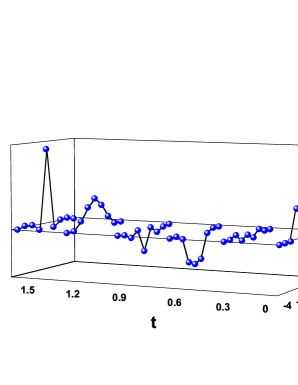
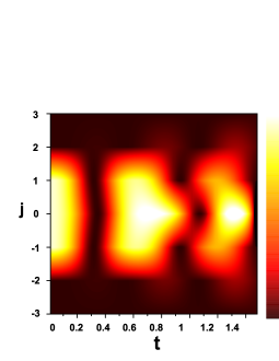
Figure 7: Left panel: escape dynamics for the $3$-units segment $Z(0)=(A,A,A)$ with $A=0.79>A_{\mathrm{crit}}$; clearly, the central unit $j=0$ is escaping from the potential well. Right panel: contour plot showing the evolution of the potential energy of the chain in the case of an initially excited $3$-units segment; the plot demonstrates the energy transfer from the adjacent units to the central unit and its localization therein. The parameters used are $\Omega_{d}^{2}=10$ ($\omega_{d}^{2}=40$, $h=0.5$) and $\beta=1$.

In the left panel of Fig. 7 we show the time evolution of the $3$-unit segment in the moderately discrete regime ($\Omega_{d}^{2}=10$), with an initial condition, $Z(0)=(A,A,A)$ where $A=0.79>A_{\mathrm{crit}}$. As shown in this panel, the segment initially performs one oscillation, but subsequently reorganizes so that at time $t\sim 1.5$ the central unit ($j=0$) has already crossed the barrier $\mathcal{U}_{\mathrm{thresh}}\sim 1.8$ and it will lead the chain to collapse. In particular, it can never return to the potential well, according to Theorem II.1, due to the autonomous nature of the system at hand.

The energy transfer from the adjacent units of the segment to the central unit (resulting in growing amplitude oscillations of this unit), is visualized in the right panel of Fig. 7. The potential energy stored in the $3$-unit segment (light colored area) is progressively localized within the central unit. The dark area between the patterns visualizes the passing from the bottom of the potential well $U_{\mathrm{min}}=0$ (with a maximal kinetic energy), as the units oscillate.

The same escape dynamics have also been confirmed numerically, for the set of parameters in the strongly discrete regime ($\Omega_{d}^{2}=100$), with the initial condition $A=0.77>A_{\mathrm{crit}}$. The collapse time in this case is $t\simeq 6.4$, which is larger compared to the respective one in the moderately discrete regime. This is expected due to the weaker interaction between the units, which results in a longer time interval during which the energy is redistributed, the more discrete the lattice becomes. Besides that, in the strongly discrete regime, the depth of the potential well is considerably increased, which has, as a result, a longer time needed for the excited units to climb over the saddle points and finally escape (cf. Fig. 1).

The analytically obtained threshold $A_{\mathrm{crit}}$, for which the segment $Z(0)=(A,A,A)$ will exhibit escape dynamics, is plotted as a function of the coupling parameter $\omega_{d}^{2}$ in Fig. 8 –see the continuous (black) line; for comparison, the numerically obtained threshold is also presented in this figure by (red) dots. The observation that $\lim_{\omega_{d}^{2}\rightarrow 0}A_{\mathrm{crit}}=\infty$ as $\omega_{d}^{2}\rightarrow 0$ reflects the fact that blow-up is not possible in the asymptotically linear regime. The numerical simulations verified the existence of a critical value $\omega^{2}_{d,\mathrm{min}}$, as we approach the asymptotically linear from the discrete regime, below which escape is prevented, and the energy stored in the $3$-units segment is dispersed along the chain leading to global existence. For large values of $\omega_{d}^{2}$ we observe that the numerical threshold converges slowly to the limit $\lim_{\omega_{d}^{2}\rightarrow\infty}A_{\mathrm{crit}}\sim 0.75$.

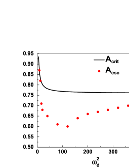
Figure 8: The analytically obtained threshold $A_{\mathrm{crit}}$, as a function of the coupling parameter $\omega_{d}^{2}$ (continuous (black) curve), against the numerical value $A_{\mathrm{esc}}$ ((red) dots) for the escape of the $3$-units segment. Other parameters used are $h=0.5$, $\beta=1$.

IV.3 Modulational instability mechanism

In this section, we will briefly review initially the modulational instability mechanism Dirk1 , with the subsequent aim to investigate its connection with escape dynamics of plane wave initial data KP92 . This will complete our program of examining blow-up for the chain starting from one site excitations and progressively passing to few and finally to many site excitations.

The modulation instability mechanism concerns the instability of a plane wave of the form

$$U_{n}=\Phi_{0}e^{i(qn-\omega t)}+\hbox{c.c},$$ (4.29)

under small perturbations of different wave numbers. When this instability occurs, the exponential growth of the perturbations creates localized excitations. The question at hand here is if a sizeable growth of the perturbations may create a critical localized excitation which, in turn, may lead to escape dynamics. Let us recall first that in the linear limit $\beta=0$ of (2.2), the existence of plane waves (4.29) is associated with the dispersion relation:

$$\omega^{2}=4\epsilon\sin^{2}\left(\frac{q}{2}\right)+\omega_{d}^{2}.$$ (4.30)

For $q=0$ and $q=\pi$, (4.30) gives $\omega^{2}=\omega_{d}^{2}$ and $\omega^{2}=\omega_{d}^{2}+4\epsilon$ respectively. Thus, the linear spectrum has a gap of size $\omega_{d}$, and is bounded by the frequency $\omega_{\mathrm{max}}^{2}=\omega_{d}^{2}+4\epsilon$.

In the nonlinear case $\beta>0$, we seek for solutions of (2.2) of the form

$$U_{n}(t)=\phi_{n}(t)e^{-i\omega_{d}t}+\hbox{c.c},\;\;\phi_{n}\in\mathbb{C},$$ (4.31)

where $\phi_{n}(t)$ denotes the varying envelope. Substitution of (4.31) into (2.2) implies that the varying envelope $\phi_{n}(t)$ satisfies the equation

$$\ddot{\phi_{n}}-2i\omega_{d}\dot{\phi_{n}}-\omega_{d}^{2}\phi_{n}=\epsilon(\phi_{n+1}-2\phi_{n}+\phi_{n-1})-\omega_{d}^{2}\phi_{n}+\beta\omega_{d}^{2}\left(3|\phi_{n}|^{2}\phi_{n}+\phi_{n}^{3}e^{2i\omega_{d}t}\right)+\hbox{c.c}.$$ (4.32)

Under the assumption of the slow-variation in time of $\phi_{n}(t)$ with respect to the main oscillation at frequency $\omega_{d}$, i.e., $\dot{\phi}_{n}<<\omega_{d}\phi_{n}$, in the rotating-wave approximation, we may keep only the terms proportional to $e^{\pm i\omega_{d}t}$; this way, (4.32) results in the DNLS equation:

$$2i\omega_{d}\dot{\phi_{n}}+\epsilon(\phi_{n+1}-2\phi_{n}+\phi_{n-1})+3\beta\omega_{d}^{2}|\phi_{n}|^{2}\phi_{n}=0.$$ (4.33)

We proceed by seeking solutions of (4.33) of the form:

$$\phi_{n}(t)=\phi_{0}e^{i\theta_{n}},\;\;\theta_{n}(t)=\,qn-\tilde{\omega}t,\;\;\phi_{0}\in\mathbb{R}.$$ (4.34)

Inserting (4.34) in (4.33), we obtain

$$2\omega_{d}\tilde{\omega}\phi_{0}e^{i\,qn}+\epsilon\phi_{0}\left(e^{i\,q(n+1)}-2e^{i\,qn}+e^{i\,q(n-1)}\right)+3\beta\omega_{d}^{2}|\phi_{0}|^{2}\phi_{0}e^{i\,qn}=0,$$

which leads to the following dispersion relation for the frequency $\tilde{\omega}$:

$$2\omega_{d}\tilde{\omega}=4\epsilon\sin^{2}\left(\frac{\,q}{2}\right)-3\beta\omega_{d}^{2}|\phi_{0}|^{2}.$$ (4.35)

In summary, the validity of the single-frequency approximation leading to the DNLS equation (4.33) for the varying envelope $\phi_{n}(t)$ of the solutions (4.31) of the DKG equation (2.2), assumes that the gap frequency $\omega_{d}$ is large compared to the other frequencies of the system,

$$4\epsilon<<\omega_{d}^{2},$$ (4.36)

and the nonlinearity is weak, in the sense:

$$\beta\phi_{0}^{2}<<1.$$ (4.37)

Having the restrictions (4.36) and (4.37) in mind, one can study the modulational instability conditions of (4.34) by considering the ansatz

$$\phi_{n}=(\phi_{0}+\chi_{n})e^{i(\theta_{n}+\psi_{n})},$$ (4.38)

where $\chi_{n}$ and $\psi_{n}$ are small perturbations of the amplitude and phase, respectively, i.e.,

$$|\chi_{n}(t)|<<\phi_{0},\;\;\hbox{and}\;\;|\psi_{n}(t)|<<|\theta_{n}(t)|.$$

Then, substituting (4.38) in the DNLS (4.33), it turns out that $\chi_{n}$ and $\psi_{n}$ satisfy the system of linear equations

$$2\omega_{d}\dot{\chi}_{n} + \epsilon\left[(\chi_{n+1}-\chi_{n-1})\sin\,q+\phi_{0}(\psi_{n+1}-2\psi_{n}+\psi_{n-1})\cos\,q\right]=0,$$ (4.39)

$$-2\omega_{d}\phi_{0}\dot{\psi_{n}} + \epsilon\left[(\chi_{n+1}-2\chi_{n}+\chi_{n-1})\cos\,q-\phi_{0}(\psi_{n+1}-\psi_{n-1})\sin\,q\right]+6\beta\omega_{d}^{2}\phi_{0}^{2}\chi_{n}=0.$$ (4.40)

Assuming that the perturbations $\chi_{n}$ and $\psi_{n}$ have the form of plane waves, namely,

$$\chi_{n}(t)=\chi_{0}e^{i(Qn-\Omega t)},$$ (4.41)

$$\psi_{n}(t)=\psi_{0}e^{i(Qn-\Omega t)},$$ (4.42)

where $\chi_{0}$ and $\psi_{0}$ are constant amplitudes, while $Q$ and $\Omega$ denote wavenumber and frequency respectively, we can derive from (4.39)-(4.40) the following system for $\chi_{0},\psi_{0}$,

$$\left(\begin{array}[]{cc}-2i(\omega_{d}\Omega-\epsilon\sin Q\sin\,q)&-4\epsilon\phi_{0}\sin^{2}\left(\frac{Q}{2}\right)\cos\,q\\ -4\epsilon\sin^{2}\left(\frac{Q}{2}\right)\cos\,q+6\beta\omega_{d}^{2}\phi_{0}^{2}&2i\phi_{0}(\omega_{d}\Omega-\epsilon\sin Q\sin\,q)\\ \end{array}\right)\cdot\left(\begin{array}[]{c}\chi_{0}\\ \psi_{0}\\ \end{array}\right)=\left(\begin{array}[]{c}0\\ 0\\ \end{array}\right).$$ (4.43)

For nontrivial solutions, we require the determinant of the matrix in (4.43) to be zero, which leads to the dispersion relation:

$$(\omega_{d}\Omega-\epsilon\sin Q\sin\,q)^{2}=\epsilon\sin^{2}\left(\frac{Q}{2}\right)\cos\,q\left(4\epsilon\sin^{2}\left(\frac{Q}{2}\right)\cos\,q-6\beta\omega_{d}^{2}\phi_{0}^{2}\right).$$ (4.44)

From this, the condition for modulation instability, i.e., for $\Omega$ with a nonvanishing imaginary part can directly be obtained from (4.44); this condition is expressed (for $\cos(q)>0$; if this sign changes, so does the sign of the inequality below) in terms of the amplitude $\phi_{0}$ and the wavenumber $Q$ as:

$$6\beta\omega_{d}^{2}\phi_{0}^{2}>4\epsilon\sin^{2}\left(\frac{Q}{2}\right)\cos q.$$ (4.45)

In the case of the mode with $q=0$, the condition for $\phi_{0}$ leading to modulational instability is:

$$\phi_{0}>\sqrt{\frac{2\epsilon\sin^{2}\left(\frac{Q}{2}\right)}{3\beta\omega_{d}^{2}}}:=\phi_{0,\mathrm{MI}}.$$ (4.46)

Condition (4.46) should be combined with restrictions (4.36) and (4.37) which, in our case, are:

$$1>>\beta\phi_{0}^{2}\;\;\hbox{and}\;\;\omega_{d}^{2}>>4\epsilon.$$ (4.47)

We also remark that in the case of modes with $0\leq q<\frac{\pi}{2}$, since

$$6\beta\omega_{d}^{2}\phi_{0}^{2}-4\epsilon\sin^{2}\left(\frac{Q}{2}\right)\cos q\geq 6\beta\omega_{d}^{2}\phi_{0}^{2}-4\epsilon,$$

instability of a plane wave occurs if

$$\phi_{0}^{2}>\frac{2}{3}\frac{\epsilon}{\beta\omega_{d}^{2}}=\frac{2}{3\beta h^{2}\omega_{d}^{2}}=\frac{2}{3\beta\Omega_{d}^{2}},\;\;\Omega_{d}^{2}=h^{2}\omega_{d}^{2},$$ (4.48)

where we have used the scaling $t\rightarrow\frac{1}{h}t$ as before.

IV.4 Small data global existence conditions and their violation

The last scenario which will be considered is based on the violation of small data, global existence conditions, and the investigation of the possible connection of this violation with the generation of instabilities. For the derivation of the conditions for global existence, which shall guarantee non-escape dynamics, we shall consider a discrete variant of the method of Ref. cazh , and use the energy functional:

$$E(t):=||\dot{U}(t)||_{\ell^{2}}^{2}+||U(t)||_{\ell^{2}_{1}}^{2}=\sum_{n=-\infty}^{+\infty}\dot{U}_{n}^{2}+\sum_{n=-\infty}^{+\infty}(U_{n+1}-U_{n})^{2}+\omega_{d}^{2}\sum_{n=-\infty}^{+\infty}U_{n}^{2},$$ (4.49)

where $||U||_{\ell^{2}_{1}}^{2}$ denotes the “linear coupling energy”-norm

$$||U||_{\ell^{2}_{1}}^{2}:=\sum_{n=-\infty}^{+\infty}(U_{n+1}-U_{n})^{2}+\omega_{d}^{2}\sum_{n=-\infty}^{+\infty}U_{n}^{2}.$$

We shall also consider the quantities

$$E_{\pm}=\frac{\omega_{d}^{2}\left[1\pm\sqrt{1-\frac{2\beta}{\omega_{d}^{2}}E(0)\left(1+\frac{\beta}{2\omega_{d}^{2}}\right)}\right]}{\beta},$$ (4.50)

which are real and positive if $E(0)$ satisfies

$$E(0)<\frac{\omega_{d}^{2}}{2\beta\left(1+\frac{\beta}{2\omega_{d}^{2}}\right)}.$$ (4.51)

Then, the small data, global existence result is stated in the following Theorem.

Theorem IV.1

We consider the energy function (4.49) and we assume that the initial data (3.2) have energy

$$E(0)<\min\left\{1,\frac{\omega_{d}^{2}}{2\beta\left(1+\frac{\beta}{2\omega_{d}^{2}}\right)}\right\}.$$ (4.52)

Then the solution of (1.3) exists globally in time ($T_{\mathrm{max}}=\infty$), and satisfies for all $t\in[0,\infty)$ the energy bound

$$E(t)<E_{-}.$$ (4.53)

Proof: See Appendix C.  $\Box$

On the other hand, if the smallness condition (4.51) is violated, i.e.,

$$E(0)>\frac{\Omega_{d}^{2}}{2\beta\left(1+\frac{\beta}{2\Omega_{d}^{2}}\right)},$$ (4.54)

the inequality (5.86) is valid for $E(t)\in[0,\infty)$ and the possibility of unbounded solutions cannot be excluded.

With this observation at hand, we may investigate the dynamics of the chain for initial data satisfying (4.54) to see if this violation condition may give an analytical value of amplitudes leading to blow-up and escape. Let us also remark that

$$\frac{\Omega_{d}^{2}}{2\beta\left(1+\frac{\beta}{2\Omega_{d}^{2}}\right)}>1\;\;\hbox{when}\;\;\Omega_{d}^{2}>\beta(1+\sqrt{2}).$$ (4.55)

IV.5 Numerical study 4: Modulational instability and violation of conditions for global existence

We conclude this section with the last numerical study, investigating the modulational instability conditions (4.46)-(4.47), and the violation of small data global existence (4.54)-(4.55). We will consider lattice parameters in the strongly discrete regime, namely, $h=0.5$ and $\omega_{d}^{2}=400$ ($\Omega_{d}^{2}=\omega_{d}^{2}h^{2}=100$), while for the nonlinearity parameter we will use the value $\beta=0.1$. We intend to examine (4.48), i.e., the conditions for modulational instability and stability for amplitudes $\phi_{0}>\phi_{0,\mathrm{MI}}$ and $\phi_{0}<\phi_{0,\mathrm{MI}}$, respectively. For our analysis we will focus on the region of modulation instability in the $(q,Q)$-plane defined in (KP92, , Fig. 2(b), pg. 3200), and particularly on the line $q=0$; in this case, the corresponding domain for the wavenumbers is $\left(0,\frac{3\pi}{4}\right)$, and we fix $Q=\frac{\pi}{2}$.

For the above set of parameters, the critical value of the amplitude $\phi_{0,\mathrm{MI}}$ defined by the right-hand side of (4.48) is:

$$\phi_{0,\mathrm{MI}}=0.18.$$ (4.56)

The violation condition (4.54) will also be tested for plane wave initial data, and we will derive the relevant critical value of the amplitude $\Phi_{0,\mathrm{crit}}$, as shown below.

The plane wave (4.29) can be rewritten as $U_{n}(t)=2\phi_{0}\cos(qn-\omega t)$ and, thus, at $t=0$:

$$U_{n}(0)=2\phi_{0}\cos qn,\;\;\mbox{and}\;\;\dot{U}_{n}(0)=2\omega\phi_{0}\sin qn,$$ (4.57)

In order to test the condition (4.54) numerically we should consider a finite lattice of $K$ units. In this case, the initial data (4.57) have initial energy $E(0):=E_{pw}(0)$ given by

$$E_{pw}(0)=4\omega^{2}\phi_{0}^{2}\sum_{n=1}^{K}\sin^{2}qn+4\phi_{0}^{2}\sum_{n=1}^{K}\left[\cos(q(n+1))-\cos qn\right]^{2}+4\phi_{0}^{2}\Omega_{d}^{2}\sum_{n=1}^{K}\cos^{2}qn.$$

It readily follows that the mode with $q=0$ has energy

$$E_{pw}(0)=4\Omega_{d}^{2}\phi_{0}^{2}K,$$ (4.58)

and the condition (4.54) will be satisfied for a chain of $K$ units if

$$\phi_{0}>\sqrt{\frac{1}{8K\beta\left(1+\frac{\beta}{\Omega_{d}^{2}}\right)}}:=\phi_{0,\mathrm{crit}}.$$ (4.59)

On the other hand, to get a $K$-independent condition for the amplitude, we first observe that the mean value of the energy $E_{pw}(0)$ of the the $q=0$ mode denoted by $\overline{E_{pw}(0)}$ is due to (4.58)

$$\overline{E_{pw}(0)}=\frac{1}{K}E_{pw}(0)=4\Omega_{d}^{2}\phi_{0}^{2}.$$

Since $E_{pw}(0)>\overline{E_{pw}(0)}$ the condition (4.54) will be satisfied for a chain of arbitrary size if

$$\overline{E_{pw}(0)}>\frac{\Omega_{d}^{2}}{2\beta\left(1+\frac{\beta}{2\Omega_{d}^{2}}\right)},$$

implying the inequality

$$\phi_{0}>\sqrt{\frac{1}{8\beta\left(1+\frac{\beta}{\Omega_{d}^{2}}\right)}}:=\Phi_{0,\mathrm{crit}}.$$ (4.60)

For the example of lattice parameters considered above, the critical value of the amplitude $\Phi_{0,\mathrm{crit}}$ is found to be

$$\Phi_{0,\mathrm{crit}}=1.11.$$ (4.61)

Note that both critical values for the amplitudes (4.56) and (4.61) are physically relevant regarding escape dynamics since in the case $\beta=0.1$ the saddle points are located $U^{\mp}_{\mathrm{max}}=\mp\frac{1}{\sqrt{\beta}}\simeq 3.16$ (and hence the initial excitation places all nodes inside their corresponding wells). It should be also recalled that the analytical condition (4.60) rigorously does not ensure global existence or escape (blow-up), since it simply violates the global existence condition (4.52) of Theorem IV.1 for plane waves. The numerical simulations below will examine whether data satisfying the analytical condition (4.60)] may lead to escape dynamics or not.

Figure 9: Evolution of the maximum energy density, normalized to the initial energy density, $V(t)$ [cf. Eq. (4.63)], of the lattice chain. The initial condition, in all three cases, is: $U_{n}(0)=2\phi_{0}+\hat{\epsilon}\cos(Qn)$, with $\hat{\epsilon}=0.005$, $Q=\frac{\pi}{2}$. The three panels correspond, respectively, to modulational stability for $\phi_{0}=0.07$ (left panel), modulational instability but without collapse for $\phi_{0}=0.15$ (middle panel), and escape dynamics for $\phi_{0}=1.25$ (right panel). The inset in the right panel shows the evolution of the maximum amplitude among the $U_{n}$, clearly demonstrating the escape at $t\simeq 4.5$.

The initial condition used in the numerical study is of the form [cf. Eq. (4.57) for $q=0$]:

$$U_{n}(0)=2\phi_{0}+\hat{\epsilon}\cos(Qn),\;\;\hat{\epsilon}<<\phi_{0},$$ (4.62)

where the amplitude of the small perturbation is $\hat{\epsilon}=0.005$.

Figure 9 demonstrates the transition from modulational stability to escape dynamics for plane wave initial data, by plotting the evolution of the ratio

$$V(t)=\max_{n}\frac{\mathcal{H}_{n}(t)}{\mathcal{H}_{n}(0)},$$ (4.63)

where the quantity

$$\mathcal{H}_{n}=\frac{1}{2}\dot{U}_{n}^{2}+\frac{1}{2}(U_{n+1}-U_{n})^{2}+\frac{\omega_{d}^{2}}{2}U_{n}^{2}-\frac{\beta\omega_{d}^{2}}{4}U_{n}^{4},$$ (4.64)

is the energy density of the system, and $\mathcal{H}_{n}(0)$ corresponds to the initial energy density, at $t=0$. The figure demonstrates the transition from modulational stability (left) to modulational instability (middle) and finally to self-organized escape (right) upon varying the amplitude $\phi_{0}$, as is explained in more detail below.

The left panel of Fig. 9 shows the evolution of (4.63) for $\phi_{0}=0.07<\phi_{0,\mathrm{MI}}$ and justifies (for this choice) the modulational stability of the plane wave; we observe that $V(t)$ shows a small fluctuation around its initial value $V(0)=1$, thus depicting the stability of the configuration over the entire time interval of the numerical integration of the system ($1000$ time units). Note that the same behavior was found for other values of the amplitude $\phi_{0}$, up to $\phi_{0}<0.15$.

The situation changes drastically for $\phi_{0}=0.15$: beyond this value, modulational instability starts manifesting itself, as shown in the middle panel of Fig. 9. The onset of the instability is characterized by a significant increase of $V(t)$ from its initial value $V(0)=1$ (an order of magnitude larger than that observed in the previous case), which implies exponential growth of the excited mode. We mention that $\phi_{0}=0.15<\phi_{0,\mathrm{MI}}=0.18$; this deviation is expected due to the approximate description of the initial equation (2.2) by the DNLS model (4.33). The long-time behavior of the system, in this modulationaly unstable regime, is shown in Fig. 10 (the parameter values, as well as the initial condition, are the same with the ones in the middle panel of Fig. 9). The contour plot of the energy density $\mathcal{H}_{n}$ [cf. Eq. (4.64)] reveals that up to $t\simeq 2000$ a periodic pattern is formed, due to the modulational-instability-induced exponential growth of the excited mode. This is a so-called breather lattice (see e.g. avadh for a relevant discussion of such waveforms in integrable models where they exist in analytically tractable form). However, after $t=2000$, and due to the highly nontrivial dynamical interactions of such modes coming into play, at this stage, we observe the formation of moving breathers, each of which acquiring a small fraction of the total amount of energy. These breathers interact with each other and exchange energy; during this process, it is observed that some “prevailing” breathers (the ones with the larger energy) seem to “absorb” the energy of the breathers that they interact with. This process continues for a long time leading to a gradual coarsening of the chain dynamics. Such processes have been debated at considerable length for Hamiltonian systems (with and without $\ell^{2}$ norm conservation properties); a recent example of such a discussion containing an account of earlier work can be found in iubini . In our long time dynamics, one can clearly identify three strong “eventual” breathers; these are located far enough from each other, so that no interactions between them are observed (at least until the end of the simulation, at $t=10,000$). A similar effect has also been observed in Ref. nln (see Fig. 7 of this work and also references therein).

The relevant evolution also brings forth the potential for connections of case examples such as that of Fig. 10 with chaotic dynamics. In particular, what we can see here, but also in Figs. 2 and 7 of nln , is that the MI manifestation leads not just to a simple unstable wavenumber, but rather to a band of unstable wavenumbers. The dominant one among them leads transiently to the formation of a structure resembling a breather lattice avadh , but as shown in both of the above examples, as well as in Figs. such as Fig. 3 of avadh , such states are unstable. Thus, the excitation of all the additional unstable modes eventually through an apparently chaotic evolution mixing these modes, leads to a self-organizing end result whereby a few dominant/robust discrete breather structures finally prevail.

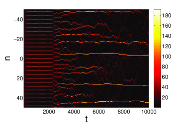
Figure 10: Contour plot, showing the long time evolution of the energy density $\mathcal{H}_{n}$, for the same initial condition as in the middle panel of Fig. 9. Up to $t\sim 2000$, the chain follows a periodic (breather lattice) pattern due to the exponential growth of the initially excited mode. Beyond that point, we observe the creation of small breathers which collide and exchange energy. At the end of the simulation ($t=10,000$), the total energy density is chiefly distributed among only $3$ distinct localized breathers.

$\Phi_{0,\mathrm{crit}}=1.11$
K	$20$	$50$	$100$	$200$	$400$	$1000$
$\phi_{0}$	$0.98$	$0.98$	$0.90$	$0.90$	$0.90$	$0.90$

Table 1: The numerically found critical amplitude $\phi_{0}$ for escape dynamics for various numbers $K$ of lattice sites. Here, $\Phi_{0,\mathrm{crit}}=1.11$ is the corresponding $K$-independent analytical prediction.

Let us now discuss the connection of the modulational instability mechanism with the emergence of escape dynamics. Generally, modulational instability gives rise to an exponential growth of the plane wave perturbations and, as a result, a large-amplitude localized mode –composed by one or few oscillators– may be formed. However, the modulational instability mechanism is not enough by itself to ensure escape dynamics, and modulationally unstable states corresponding to localized, even chaotic excitations, may exist globally in time. Our numerical simulations have shown that there exists a threshold of the amplitude $\phi_{0}$ separating the modulational instability regime from the escape dynamics regime; this threshold was found to be (for the set of parameters used in Fig. 9) $\phi_{0}=0.98$. The right panel of Fig. 9 depicts the evolution of (4.63) for $\phi_{0}=1.25$, i.e., beyond the threshold value. It is observed that for a short time interval $V(t)$ remains close to its initial value while, at a later time, a sudden and sharp increase appears; this is also associated with a sharp increase of the maximum amplitude along the chain, leading to the escape from the potential well of the critical unit possessing this amplitude. The inset in the right panel of Fig. 9 shows the evolution of $\max_{n}|U_{n}(t)|$ crossing the saddle point barrier.

It is interesting to observe, that the analytical value $\Phi_{0,\mathrm{crit}}$ [cf. Eq. (4.61)] appears to yield a value proximal to the amplitude threshold separating the modulational instability from the escape dynamics regime. We have confirmed numerically that an initial condition of the form of a randomly perturbed plane wave, namely,

$$U_{n}(0)=2\Phi_{0,\mathrm{crit}}+\tilde{\epsilon}\cdot\mathrm{noise},\;\;\tilde{\epsilon}=10^{-4},$$ (4.65)

leads to escape dynamics and blow-up in finite time, and the evolution of $V(t)$ is similar to the one shown in the right panel of Fig. 9. Additionally, it should be noted that our simulations have also confirmed the fact that $\Phi_{0,\mathrm{crit}}$ is almost independent of the number $K$ of lattice sites, as seen in Table 1: it is clearly observed that the numerically found critical amplitude takes the constant value $\phi_{0}=0.90$ for chains composed by more than $K=100$ sites (and up to $K=1000$), while it takes a slightly larger value for smaller chains.

The linearly damped system: Transient modulational instability within the exponential decay of solutions. In the case of the linearly damped system (3.5), seeking for solutions (4.31) under the slow-variation in time approximation, we derive the linearly damped analogue of the DNLS (4.33), which is

$$i\omega_{d}\dot{\phi_{n}}+i\omega_{d}\frac{\gamma}{2}\phi_{n}+\epsilon(\phi_{n+1}-2\phi_{n}+\phi_{n-1})+\frac{3}{2}\beta\omega_{d}^{2}|\phi_{n}|^{2}\phi_{n}=0.$$ (4.66)

Multiplying (4.66) by $\bar{\phi}_{n}$ and summing over $n$ (in the infinite lattice or in the finite lattice subject to Dirichlet or periodic boundary conditions), we derive the equation

$$\frac{1}{2}\frac{d}{dt}||\phi||^{2}_{\ell^{2}}+\frac{\gamma}{2}||\phi||^{2}_{\ell^{2}}=0,$$

implying the decay of the $\ell^{2}$-norm

$$||\phi(t)||^{2}_{\ell^{2}}=e^{-\gamma t}||\phi(0)||^{2}_{\ell^{2}},$$ (4.67)

for all solutions of the approximating DNLS equation (4.66). Furthermore, (4.67) and the norm relations (2.14) and (2.15) imply for both the cases of the infinite or the finite lattice, the sup-norm decay estimate

$$||\phi(t)||^{2}_{\infty}\leq e^{-\gamma t}||\phi(0)||^{2}_{\ell^{2}}.$$ (4.68)

Hence $\lim_{t\rightarrow\infty}||\phi(t)||_{\infty}=0$, and all solutions of (4.66) decay at an exponential rate, independently of the initial data. However, the spatially uniform decay estimate (4.68) does not exclude a possible transient growth of perturbations, and consequently, a transient modulational instability behavior within the frame of exponential decay. This transient modulational instability is especially expected to be noticeable for small values of damping.

The above suggestions have been tested numerically, by considering the evolution of the damped DKG chain (3.5) with perturbed plane wave initial data (4.62). The values of parameters for $h$, $\beta$, $\omega_{d}^{2}$ and $Q$, are the same as in the numerical study performed for the Hamiltonian system $\gamma=0$. The amplitude is $\phi_{0}=0.15$, inducing modulation instability in the Hamiltonian case. The two top panels of Fig. 11 show the contour plots of the energy density $\mathcal{H}_{n}$ of the dissipative system for $\gamma=2$ (left panel) and $\gamma=0.02$ (right panel), respectively. Although in both cases the solutions decay to zero as the approximating DNLS estimate (4.68) suggests, in the right panel we observe the formation of a transient breather lattice, which survives the exponential decay up to $t\simeq 100$. The same breather lattice lives only up to $t\simeq 1$, as shown in the top left panel, due to the stronger damping $\gamma=2$. The two bottom panels show the contour plot of the difference $\mathcal{H}_{n}\left[U_{n}|_{\gamma>0}\right]-\mathcal{H}_{n}\left[U_{n}|_{\gamma=0}\exp(-\gamma t)\right]$, i.e., of the energy density $\mathcal{H}_{n}\left[U_{n}|_{\gamma>0}\right]$ for the damped system (3.5) from the energy density $\mathcal{H}_{n}\left[U_{n}|_{\gamma=0}\exp(-\gamma t)\right]$, where $U_{n}|_{\gamma=0}$ denotes the solution of the Hamiltonian system (2.2). In the bottom right panel the time evolution of the energy density difference is shown for the damping value $\gamma=0.02$. The peaks observed therein, within the time interval $[20,150]$, illustrate a transient modulation instability regime, where localization of energy and formation of a lattice of localized modes occurs. In the case of stronger damping $\gamma=2$, the transient instability regime is hardly observable. Numerical simulations for smaller values of $\gamma$ depict that the transient modulation instability regime is increased, as it is expected when the Hamiltonian limit $\gamma\rightarrow 0$ is approached.

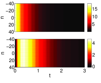
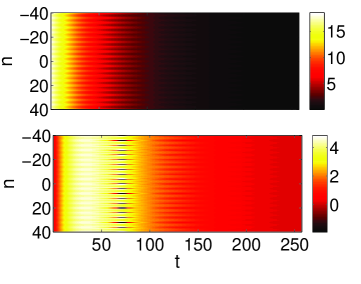
Figure 11: The top panels show the long time evolution of the energy density $\mathcal{H}_{n}$ for the linear damped lattice $\gamma>0$. The bottom panels show the long time evolution of the difference $\mathcal{H}_{n}\left[U_{n}|_{\gamma>0}\right]-\mathcal{H}_{n}\left[U_{n}|_{\gamma=0}\exp(-\gamma t)\right]$, i.e., of the energy density $\mathcal{H}_{n}\left[U_{n}|_{\gamma>0}\right]$ for the damped lattice from the energy density $\mathcal{H}_{n}\left[U_{n}|_{\gamma=0}\exp(-\gamma t)\right]$. The left panels are for $\gamma=2$ and the right panels for $\gamma=0.02$. The initial condition is: $U_{n}(0)=2\phi_{0}+\hat{\epsilon}\cos(Qn)$, with $\hat{\epsilon}=0.005$, $Q=\frac{\pi}{2}$ and $\phi_{0}=0.15$. A transient modulational instability regime within the time interval $[20,150]$ is evident in the bottom right panel.

V Discussion and conclusions

In this work, we have studied the escape problem in the discrete repulsive $\phi^{4}$-model. We have considered both the Hamiltonian ($\gamma=0$) and the dissipative ($\gamma>0$) variants of the model. We have assumed different types of initial conditions, ranging from single-excited units and small segments to plane waves. Our results address several relevant points related to the problem, as is briefly described below.

In the Hamiltonian case, we have discussed how the system falls within the class of abstract second order evolution equations of divergent structure. Such systems can be treated, with respect to global non-existence, by the energy methods of Ref. GP , involving the formulation of suitable differential inequalities enabling the identification of conditions for blow-up. For initial data in the form of a single-unit excitation (all other units being initially located in the minimum $U_{\mathrm{min}}=0$), it is intuitively expected that escape occurs if the total energy of this unit is (sufficiently) greater than the energy barrier $E_{\mathrm{max}}$, i.e., the initial position of the unit is located outside the potential well. Indeed, we have derived a suitable analytical value for the initial position of the single unit outside the well, which serves as a sufficient condition for the absence of global existence. However, these single-site initial data are very relevant for two important questions related to escape dynamics (already posed in Refs. Dirk1 ; Dirk2 ): is it possible that the neighbors coupled to the escaping unit also get driven over the barrier and give rise to a concerted escape of the entire chain ? As an alternative scenario, can this escaping unit even be pulled back into the domain of attraction by the restoring coupling forces ? We have definitively shown that both the drive over and the pull back effects can be realized in numerical experiments of such chains.

At this point, it should be remarked that the autonomy of the system allows to discuss the derived conditions in terms of the fate of the unit of the critical mode which, at a specific time, escapes from the well. In other words, time-invariance allows for posing as initial condition the position and momenta of the chain at an escaping snapshot, and consider as an initial time, any time referred to this barrier-crossing snapshot.

The numerical simulations performed in Section II.1 justified that the analytical conditions capture the qualitative behavior of the chain and its dependence on the strength of the binding forces. Blow-up occurs when the analytical prediction is satisfied and a concerted escape follows when we are in the regime where the role of the coupling is significant. On the contrary, if the analytical condition is not satisfied then for suitable initial conditions, the initially out-of-well unit may be pulled back by the neighbors inside the stability domain, leading the initially escaping “spike-like” mode to give rise to a waveform which will exist globally in time. Furthermore, the numerical simulations revealed the existence of a “true” threshold for the position of the excited unit outside of the well, acting as a separatrix between the above two distinct dynamical behaviors. For this numerical threshold, the $\omega_{d}^{2}$-dependent analytical prediction serves as an upper bound, with a justifiable error in the regime ranging from moderate to very strong discreteness. Both theory and numerics suggest that the threshold position moves far from the position of the saddles in the continuum limit.

In the same setting, we have also examined the global existence result of (GP, , Lemma 2.1, pg. 455), addressing the following question. Assuming negative time derivative of the $\ell^{2}$ norm, while keeping the non-positivity condition of the initial Hamiltonian energy, does global existence arise for the solutions ? The answer we found is that the system under consideration [cf. Eqs. (1.3)-(1.4)] serves as a counter-example for the aforementioned global existence result, a feature confirmed by our numerical simulations.

We have also studied the linearly damped system [cf. Eq. (1.3) with $\gamma>0$], for which the questions posed on the effect of the strength of the binding forces and their interplay with nonlinearity are additionally complicated by the role of damping. In that regard, we have tried to answer the following question: can the appearance of damping affect the position threshold which separates collapse from global existence ? To examine the above question, we have applied on (1.3) suitable modifications of the energy methods developed in Ref. PS98 . These methods have enabled us to provide a $\gamma$-independent prediction for the position threshold of the single excited unit, and the numerical experiments of section III.1 have verified this independence. Theoretical and numerical evidence has also been provided for the improvement that this analytical estimate yields in connection to the true threshold.

We have also examined the escape phenomenon for multi-site excitations inside the respective wells, trying to answer the following questions: is it possible to describe escape scenarios for such initial excitations ? Also, is it possible to derive quantitative conditions for these excitations (e.g., initial positions, initial amplitudes) which are sufficient for escape ? These questions were answered in the positive by using suitable modifications of our energy arguments. Finally, for plane wave excitations, relevant answers were provided by the analysis of the modulational instability mechanism.

Motivated by the fact that escape is a phenomenon characterized by the concentration of energy within confined segments of the chain, in Section IV.1 we have examined the evolution of a lattice segment of unit length. With an appropriate cut-off argument, we have derived a condition on the initial “energy” of the segment (in terms of the $\ell^{4}$-norm). Although this condition formally is not establishing collapse by itself, heuristic arguments based on the violation of the invariance principles of potential wells PS73 ; PSrev , indicate that it is relevant for initiating escape in the discrete regime. The numerical results validated the theoretical expectations and enabled us to recover the parametric regimes on which the escape process may be observed for our finite segment of excited initial data.

Finally, we have examined escape, in terms of the instabilities of plane wave initial conditions (Section IV). In that regard, we have reviewed the derivation of the modulational instability condition for the amplitude of plane waves KP92 , based on the DNLS approximation of the slowly-varying envelope solutions. On the other hand, as explained above, analytical energy arguments and direct numerical simulations revealed the existence of three different regimes for the plane wave amplitudes: modulational stability, modulational instability without escape, and modulational instability accompanied by escape. For the linearly damped DKG chain, the numerical results verified a transient modulation instability regime. The instabilities will be completely suppressed ultimately, in accordance with the predictions of the damped DNLS approximation.

It is crucial to remark that modulational instability analysis structurally cannot be used for the examination of the self-organized escape dynamics for the DKG chain; the latter, is associated with blow-up in finite time (equivalent to the escape time when the initial data are in the potential well), while the modulational instability analysis relies on an approximation based on the use of the DNLS equation (4.33); for the latter, solutions always exist globally in time, independently of the initial data and the strength of the nonlinear term KY1 ; Wein99 . This is a vast difference between the DNLS and DKG systems. Regarding the collapse behavior, the DKG demonstrates some analogies with its continuous counterpart, i.e., the nonlinear KG partial differential equation (PDE), which also may exhibit collapse depending on the size of the initial data and the strength of nonlinearity. Such analogies between DNLS and NLS equations are limited only to one spatial dimension and restrictively to the case of the cubic nonlinearity; in the case of focusing, power-type nonlinearities $f(z)=|z|^{2p}z$, solutions of the one-dimensional NLS PDE may blow-up in finite time when $p\geq 2$, depending on the size and type of initial data cazh , even in the linearly damped case tsu . Furthermore, in view of the modulation stability analysis, it should be recalled that the DNLS approximation drastically modifies the results concerning the stability domains, which may be deduced from a continuous NLS PDE approximation. In particular, it has been illustrated in KP92 , that a stability analysis based on the continuous NLS approximation (the analogue of Eq. (4.44) for $q,Q<<1$) may fail, by erroneously predicting stability in regions of modulation instability which are correctly detected by the DNLS analogue. Modulation instability effects appear in the NLS PDE equation with dissipation as it was shown, e.g., in Refs. RKDM ; segur ; depending on the type and the size of the damping, modulation instability effects may be considerable.

The results presented in this work may pave the way for future work in many interesting directions. Below, we briefly present a few such examples.

• A natural possibility is to extend the present considerations to higher dimensional settings, where the role of the coupling will be more significant due to the geometry enforcing additional neighbors.

• It is also relevant to consider via the methods and diagnostics presented herein the phenomenology of different types of potentials including e.g., the Morse potential, which is relevant to DNA denaturation as modeled by the Peyrard-Bishop model PB . We speculate that the techniques used herein may turn out to be more broadly relevant to problems involving hydrogen-bonds and, more generally, aspects of molecular dissociation.

• While the present study has focused on cubic nonlinearities, it might also be of interest to consider quintic nonlinearities in the one-dimensional problem, or cubic ones in the two-dimensional case. In the present case, the DKG model is structurally closer to its continuum analog (regarding collapse properties) or to the DNLS (regarding MI features– but the DNLS model does not have collapse due to the conservation of the $\ell^{2}$ norm). However, for the NLS equation in the continuum case, it is well-known susu that a quintic nonlinearity is the threshold for collapsing dynamics in 1d, while the cubic one is the corresponding threshold for 2d. Hence, for such models comparing/contrasting the collapse features of the lattice (DKG) model with the continuum (NLS) PDE problem would be of interest in its own right.

• Finally, it is certainly relevant, following similar lines of approach as the work of Dirk1 ; Dirk2 to attempt to quantify the effects of noise in these systems and generalize in a probabilistic way the deterministic statements about escape presented herein for noise realizations with different correlation properties.

Such studies are currently in progress and will be presented in future publications.

APPENDICES: Proofs of global non-existence and small data global existence results for the system (1.3)

In this complementary section, we provide the proofs of the analytical results concerning the global non-existence conditions, as well as the small data global existence conditions for the system (1.3).

We start our considerations from the local in time existence of solutions. Let us recall from (K2, , pg. 468) that (1.3)-(1.4) can be formulated as an abstract evolution equation in $\ell^{2}\times\ell^{2}$ (see Ball1b ; cazh for the continuous analogue). For instance, we may set $\mathbf{\hat{A}}:=\Delta_{2}-\omega_{d}^{2}$, and check that the operator

$$\mathbf{B}:=\left[\begin{array}[]{cc}0&1\\ \mathbf{\hat{A}}&0\end{array}\right],\;\;D(\mathbf{B}):=\left\{\left[\begin{array}[]{l}z\\ \omega\end{array}\right]\,:\,z,\omega\in\ell^{2},\,\mathbf{\hat{A}}z\in\ell^{2}\right\},$$ (5.1)

is a skew-adjoint operator, since

$$\mathbf{B}^{*}:=-\left[\begin{array}[]{cc}0&1\\ \mathbf{\hat{A}}&0\end{array}\right],\;\;D(\mathbf{B}^{*}):=\left\{\left[\begin{array}[]{l}\chi\\ \zeta\end{array}\right]\,:\,\chi,\zeta\in\ell^{2},\,\mathbf{\hat{A}}\chi\in\ell^{2}\right\},$$

and $D(\mathbf{B})=D(\mathbf{B}^{*})$. The operator $\mathbf{B}$, is the generator of an isometry group $\mathcal{T}(t):\mathbb{R}\rightarrow\mathcal{L}(\ell^{2}\times\ell^{2})$ –the space of linear and bounded operators of $\ell^{2}\times\ell^{2}$. Setting

$$\mathbf{U}=\left[\begin{array}[]{c}U\\ \dot{U}\end{array}\right],\;\;\mathbf{F}(\mathbf{U})=\left[\begin{array}[]{c}0\\ \beta\omega_{d}^{2}U^{3}\end{array}\right],$$

equation (1.3) can be rewritten as

$$\dot{\mathbf{U}}=\mathbf{B}\mathbf{U}+\mathbf{F}(\mathbf{U}).$$ (5.2)

In the above set-up, fixing $T>0$ and considering initial data $\mathbf{U}(0)=[U(0),\dot{U}(0)]^{\mathrm{T}}\in\ell^{2}\times\ell^{2}$, a function $\mathbf{U}(t):=[U(t),\dot{U}(t)]^{\mathrm{T}}\in\mathrm{C}([0,T],\ell^{2}\times\ell^{2})$ is a solution of (5.2), if and only if

$$\mathbf{U}(t)=\mathcal{T}(t)\mathbf{U}(0)+\int_{0}^{t}\mathcal{T}(t-s)\mathbf{F}(\mathbf{U}(s))ds:=S(t)\mathbf{U}(0).$$ (5.3)

The nonlinear term defines a locally Lipschitz map $\mathbf{F}:\ell^{2}\times\ell^{2}\rightarrow\ell^{2}\times\ell^{2}$ and Eq. (5.3) can be treated exactly as in (KY1, , Theorem 2.1, pg. 94) in order to prove the following.

Theorem V.1

(a) For all $\mathbf{U}(0)\in\ell^{2}\times\ell^{2}$, there exists $T_{\mathrm{max}}(\mathbf{U}(0))>0$ and a function $\mathbf{U}(t)\in\mathrm{C}([0,T_{\mathrm{max}}),\ell^{2}\times\ell^{2})$ which is for all $0<T<T_{\mathrm{max}}$, the unique solution of (5.2) in $\mathrm{C}([0,T],\ell^{2}\times\ell^{2})$ (well posedness).
(b)  The following alternatives exist: (i) $T_{\mathrm{max}}=\infty$, or (ii) $T_{\mathrm{max}}<\infty$ and

$$\lim_{T\uparrow T_{\mathrm{max}}}||\mathbf{U}(t)||_{\ell^{2}\times\ell^{2}}=\infty,\;\;\mbox{(maximality)}.$$

(c) The unique solution depends continuously on the initial data: If $\{\mathbf{U}_{n}(0)\}_{n\in\mathbb{N}}$ is a sequence in $\ell^{2}\times\ell^{2}$ such that $\mathbf{U}_{n}(0)\rightarrow\mathbf{U}(0)$ and if $T<T_{\mathrm{max}}$, then $S(t)\mathbf{U}_{n}(0)\rightarrow S(t)\mathbf{U}(0)$ in $\mathrm{C}([0,T],\ell^{2}\times\ell^{2})$.

Let us remark that for the local existence of solutions for (3.1)-(3.2) we have the same result of Theorem V.1. For its proof we just have to replace the matrix operator (5.1) with the matrix operator:

$$\mathbf{B}_{\gamma}:=\left[\begin{array}[]{cc}0&1\\ \mathbf{\hat{A}}&-\gamma\end{array}\right],\;\;D(\mathbf{B}):=\left\{\left[\begin{array}[]{l}z\\ \omega\end{array}\right]\,:\,z,\omega\in\ell^{2},\,\mathbf{\hat{A}}z\in\ell^{2}\right\}.$$ (5.4)

Appendix A: Proof of Theorem II.1

We start by observing that the Hamiltonian can be written in the Lagrangian form

$$\mathcal{H}(t)=\frac{1}{2}||\dot{U}||_{\ell^{2}}^{2}-V(U),$$ (5.5)

where

$$V(U):=-\frac{1}{2}\sum_{n=-\infty}^{+\infty}(U_{n+1}-U_{n})^{2}-\frac{\omega_{d}^{2}}{2}\sum_{n=-\infty}^{+\infty}U_{n}^{2}+\frac{\beta\omega_{d}^{2}}{4}\sum_{n=-\infty}^{+\infty}U_{n}^{4}.$$ (5.6)

The functional $V:\ell^{2}\rightarrow\mathbb{R}$ is differentiable (see (K1, , Lemma 2.3, pg. 121)), and for the derivative $V^{\prime}(U)$ at $U\in\ell^{2}$, it holds that

$$(V^{\prime}(U),Y)_{\ell^{2}}=-\sum_{n=-\infty}^{+\infty}(U_{n+1}-U_{n})(Y_{n+1}-Y_{n})-\omega_{d}^{2}\sum_{n=-\infty}^{+\infty}U_{n}Y_{n}+\beta\omega_{d}^{2}\sum_{n=-\infty}^{+\infty}U_{n}^{3}Y_{n},\;\;\mbox{for all}\;\;W\in\ell^{2}.$$ (5.7)

Furthermore, by setting $Y=U$ in (5.7), we get that

$$(V^{\prime}(U),U)_{\ell^{2}}=-\sum_{n=-\infty}^{+\infty}(U_{n+1}-U_{n})^{2}-\omega_{d}^{2}\sum_{n=-\infty}^{+\infty}U_{n}^{2}+\beta\omega_{d}^{2}\sum_{n=-\infty}^{+\infty}U_{n}^{4}.$$ (5.8)

With these preparations we proceed in various steps.
Step 1: The inequality

$$(V^{\prime}(U),U)-4V(U)\geq 0,\;\;\mbox{for all}\;\;U\in\ell^{2},$$ (5.9)

holds. Indeed, we see from (5.6) and (5.7), that

$$(V^{\prime}(U),U)_{\ell^{2}}-4V(U)=\sum_{n=-\infty}^{+\infty}(U_{n+1}-U_{n})^{2}+\omega_{d}^{2}\sum_{n=-\infty}^{+\infty}U_{n}^{2}\geq 0.$$ (5.10)

Thus the claim (5.9) is proved.
Step 2: The function $x(t)=||U(t)||^{2}_{\ell^{2}}$ satisfies the relations

$$\dot{x}(t) = 2(U(t),\dot{U}(t))_{\ell^{2}},$$ (5.11)

$$\ddot{x}(t) \geq 2||\dot{U}||_{\ell^{2}}^{2}+8V(U).$$ (5.12)

Equation (5.11) follows by direct differentiation of $x(t)=||U(t)||^{2}_{\ell^{2}}=\sum_{n=-\infty}^{+\infty}U_{n}(t)U_{n}(t)$. Note that all differentiations in the proof are justified by the local existence theorem of solutions in the interval $[0,T_{\mathrm{max}})$ of local existence.

For the inequality (5.12) we first differentiate (5.11) with respect to time and we substitute the expression $\ddot{U}$ from the system (1.3), which will be written for brevity as $\ddot{U}=\Delta_{2}U-\omega_{d}^{2}U+\beta\omega_{d}^{2}U^{3}$. Indeed, we have

$$\ddot{x}(t) = 2(\dot{U},\dot{U})_{\ell^{2}}+2(U,\ddot{U})_{\ell^{2}}$$ (5.13)

$$= 2||\dot{U}||_{\ell^{2}}^{2}+2(U,\Delta_{2}U-\omega_{d}^{2}U+\beta\omega_{d}^{2}U^{3})_{\ell^{2}}$$

$$= 2||\dot{U}||_{\ell^{2}}^{2}+2(V^{\prime}(U),U)_{\ell^{2}}.$$

Next, by using the inequality (5.9) of Step 1, which implies that $(V^{\prime}(U),U)_{\ell^{2}}\geq 4V(U)$, we estimate the second term of the right (5.13) as

$$\ddot{x}(t)\geq 2||\dot{U}||_{\ell^{2}}^{2}+2(V^{\prime}(U),U)_{\ell^{2}}\geq 2||\dot{U}||_{\ell^{2}}^{2}+8V(U).$$

Hence, the inequality (5.12) is proved.
Step 3: Assume that the initial Hamiltonian is $H(0)\leq 0$. Then it holds that

$$\ddot{x}(t)\geq 6||\dot{U}||^{2}_{\ell^{2}}\geq 0.$$ (5.14)

To prove (5.14), we observe first that the equivalent expression (5.5) for the Hamiltonian implies that

$$V(U)=\frac{1}{2}||\dot{U}||^{2}_{\ell^{2}}-\mathcal{H}(t).$$ (5.15)

Due to the conservation of the Hamiltonian $\mathcal{H}(t)=\mathcal{H}(0)$, (5.15) can be rewritten as

$$V(U)=\frac{1}{2}||\dot{U}||^{2}_{\ell^{2}}-\mathcal{H}(0).$$ (5.16)

By replacing the term $V(U)$ of the inequality (5.12) proved in Step 2 with the right-hand side of (5.16), we have that

$$\ddot{x}(t)\geq 2||\dot{U}||_{\ell^{2}}^{2}+8\left(\frac{1}{2}||\dot{U}||^{2}_{\ell^{2}}-\mathcal{H}(0)\right).$$ (5.17)

Since $\mathcal{H}(0)\leq 0$ by assumption, from (5.17) we derive the inequality

$$\ddot{x}(t)\geq 2||\dot{U}||_{\ell^{2}}^{2}+8\left(\frac{1}{2}||\dot{U}||^{2}_{\ell^{2}}\right)=6||\dot{U}||^{2}_{\ell^{2}}\geq 0.$$

Hence (5.14) is proved.
Step 4: Under the assumption $\mathcal{H}(0)\leq 0$, the norm function $x(t)=||U(t)||_{\ell^{2}}^{2}$ satisfies the differential inequality

$$\ddot{x}(t)\geq\frac{3}{2}\frac{[\dot{x}(t)]^{2}}{x(t)}.$$ (5.18)

To prove (5.18), we observe first that the Cauchy-Schwarz inequality implies the estimate

$$[\dot{x}(t)]^{2}=[2(U,\dot{U})_{\ell^{2}}]^{2}\leq 4||U||^{2}_{\ell^{2}}||\dot{U}||^{2}_{\ell^{2}}=4x(t)||\dot{U}||^{2}_{\ell^{2}},$$

which can be written as

$$||\dot{U}||^{2}_{\ell^{2}}\geq\frac{[\dot{x}(t)]^{2}}{4x(t)}.$$ (5.19)

Then, from a combination of (5.14) and (5.19), the inequality (5.18) readily follows.
Step 5 (finite-in time-singularity): In this final step for the proof of the theorem we shall use together with the assumption for negative initial Hamiltonian $\mathcal{H}(0)\leq 0$, the additional assumption $\dot{x}(0)=2(U(0),\dot{U}(0))_{\ell^{2}}>0$ (positive time derivative/increase of the $\ell^{2}$ norm initially). Under these assumptions, $\dot{x}(t)>0$ in the interval $[0,T_{\mathrm{max}})$ of existence and $x(t)=||U(t)||_{\ell^{2}}^{2}$ is strictly increasing in the interval of existence.

Indeed, from the inequality (5.14) it follows that the function $\dot{x}(t)$ is increasing in the interval $[0,T]$, $T<T_{\mathrm{max}}$. Since we have assumed $\dot{x}(0)=2(U(0),\dot{U}(0)>0$ and $\dot{x}(t)$ is increasing, it readily follows that $\dot{x}(t)>0$, on $[0,T]$. Therefore, $x(t)$ is strictly increasing on $[0,T]$. The inequality (5.18), can be rewritten as

$$\frac{\ddot{x}(t)}{\dot{x}(t)}\geq\frac{3}{2}\frac{\dot{x}(t)}{x(t)}.$$ (5.20)

Note that all the quantities involved are strictly positive on $[0,T]$ as well as their initial values at $t=0$. Integrating (5.20) on $[0,t]$ for $t\leq T$, we get that

$$\ln[\dot{x}(t)]-\ln[\dot{x}(0)]\geq\frac{3}{2}\left(\ln[x(t)]-\ln[x(0)]\right),$$

which implies that

$$\frac{\dot{x}(t)}{x(t)^{\frac{3}{2}}}\geq\frac{\dot{x}(0)}{x(0)^{\frac{3}{2}}}.$$

Integrating on $[0,t]$ for $t\leq T$ once more, we get that

$$-\frac{2}{x(t)^{\frac{1}{2}}}+\frac{2}{x(0)^{\frac{1}{2}}}\geq\frac{\dot{x}(0)}{x(0)^{\frac{3}{2}}}t.$$ (5.21)

Solving (5.21) in terms of $x(t)$ we eventually derive the lower estimate

$$x(t)\geq\frac{x(0)^{4}}{\left(2x(0)^{\frac{3}{2}}-x(0)^{\frac{1}{2}}\dot{x}(0)t\right)^{2}}.$$ (5.22)

The right-hand side diverges (blows-up) at finite time

$$T_{\mathrm{b}}:=2\frac{x(0)}{\dot{x}(0)}=2\frac{||U(0)||^{2}}{(U(0),\dot{U}(0))_{\ell^{2}}},$$

the time given in (2.1). Therefore the left-hand side $x(t)=||U(t)||_{\ell^{2}}^{2}$ cannot exist more than $T_{\mathrm{b}}$.

Appendix B: Proof of Theorem III.1

Step 1 (Energy identities): Multiplying (3.1) by $\dot{U}_{n}$ and summing over $\mathbb{Z}$ (and by parts in the coupling term), we derive the energy identity

$$\frac{1}{2}\frac{d}{dt}\left\{\frac{1}{2}\sum_{n=-\infty}^{+\infty}\dot{U}_{n}^{2}+\frac{1}{2}\sum_{n=-\infty}^{+\infty}(U_{n+1}-U_{n})^{2}+\frac{\omega_{d}^{2}}{2}\sum_{n=-\infty}^{+\infty}U_{n}^{2}-\frac{\beta\omega_{d}^{2}}{4}\sum_{n=-\infty}^{+\infty}U_{n}^{4}\right\}+\gamma\sum_{n=-\infty}^{+\infty}\dot{U}_{n}^{2}=0,$$ (5.23)

which, using the definition of the Hamiltonian (1.5), can be written as

$$\frac{d}{dt}\mathcal{H}(t)+\gamma\sum_{n=-\infty}^{+\infty}\dot{U}_{n}^{2}=0.$$ (5.24)

Integrating in $[0,t]$ for any $t\in[0,T]$, $T<T_{\mathrm{max}}$ –the maximal interval of existence, we get the energy identity

$$\mathcal{H}(t)+\gamma\int_{0}^{t}||\dot{U}(s)||^{2}_{\ell^{2}}ds=\mathcal{H}(0).$$ (5.25)

Step 2 (Inequality for the Hamiltonian $\mathcal{H}(t)$): For every $t\in[0,T]$, the Hamiltonian satisfies

$$\mathcal{H}(t)\geq\frac{\omega_{d}^{2}}{2}\left(\sum_{n=-\infty}^{+\infty}U_{n}^{4}\right)^{\frac{1}{2}}-\frac{\beta\omega_{d}^{2}}{4}\sum_{n=-\infty}^{+\infty}U_{n}^{4}.$$ (5.26)

To derive (5.26), we first observe that

$$\frac{1}{2}\sum_{n=-\infty}^{+\infty}(U_{n+1}-U_{n})^{2}+\frac{\omega_{d}^{2}}{2}\sum_{n=-\infty}^{+\infty}U_{n}^{2}\geq\frac{\omega_{d}^{2}}{2}\sum_{n=-\infty}^{+\infty}U_{n}^{2}.$$ (5.27)

Furthermore, by applying the inequality

$$\left(\sum_{n=-\infty}^{+\infty}|U_{n}|^{p}\right)^{\frac{1}{p}}\leq\left(\sum_{n=-\infty}^{+\infty}|U_{n}|^{q}\right)^{\frac{1}{q}},\;\;\mbox{for all}\;\;1\leq q\leq p\leq\infty,$$ (5.28)

in the case $p=4$ and $q=2$, we get that

$$\left(\sum_{n=-\infty}^{+\infty}U_{n}^{4}\right)^{\frac{1}{4}}\leq\left(\sum_{n=-\infty}^{+\infty}U_{n}^{2}\right)^{\frac{1}{2}}.$$ (5.29)

Thus, we have

$$\left(\sum_{n=-\infty}^{+\infty}U_{n}^{4}\right)^{\frac{1}{2}}\leq\sum_{n=-\infty}^{+\infty}U_{n}^{2}.$$

With the above inequality at hand, we estimate the right-hand side of (5.27) from below as

$$\frac{1}{2}\sum_{n=-\infty}^{+\infty}(U_{n+1}-U_{n})^{2}+\frac{\omega_{d}^{2}}{2}\sum_{n=-\infty}^{+\infty}U_{n}^{2} \geq \frac{\omega_{d}^{2}}{2}\sum_{n=-\infty}^{+\infty}U_{n}^{2}.$$ (5.30)

$$\geq \frac{\omega_{d}^{2}}{2}\left(\sum_{n=-\infty}^{+\infty}U_{n}^{4}\right)^{\frac{1}{2}}.$$

The left-hand side of (5.30) is the sum of the coupling and quadratic $U_{n}$-dependent terms of the Hamiltonian. Since the kinetic energy term is always $\frac{1}{2}\sum_{n=-\infty}^{+\infty}\dot{U}_{n}^{2}\geq 0$, for all $t\in[0,T]$, we have due to (5.30) that

$$\mathcal{H}(t) = \frac{1}{2}\sum_{n=-\infty}^{+\infty}\dot{U}_{n}^{2}+\frac{1}{2}\sum_{n=-\infty}^{+\infty}(U_{n+1}-U_{n})^{2}+\frac{\omega_{d}^{2}}{2}\sum_{n=-\infty}^{+\infty}U_{n}^{2}-\frac{\beta\omega_{d}^{2}}{4}\sum_{n=-\infty}^{+\infty}U_{n}^{4}$$

$$\geq+\frac{1}{2}\sum_{n=-\infty}^{+\infty}(U_{n+1}-U_{n})^{2}+\frac{\omega_{d}^{2}}{2}\sum_{n=-\infty}^{+\infty}U_{n}^{2}-\frac{\beta\omega_{d}^{2}}{4}\sum_{n=-\infty}^{+\infty}U_{n}^{4}$$

$$\geq\frac{\omega_{d}^{2}}{2}\left(\sum_{n=-\infty}^{+\infty}U_{n}^{4}\right)^{\frac{1}{2}}-\frac{\beta\omega_{d}^{2}}{4}\sum_{n=-\infty}^{+\infty}U_{n}^{4}.$$

The claim (5.26) is proved.
Step 3 (Derivation of the conditions (3.3) and (3.4) and their consequences): The right-hand side of (5.26) defines a functional for the scalar continuous function $x(t)=||U(t)||_{\ell^{4}}=\left(\sum_{n=-\infty}^{+\infty}U_{n}^{4}\right)^{\frac{1}{4}}$. This functional is of the repulsive $\phi^{4}$-type. For instance, (5.26) can be written in the short-hand notation

$$\mathcal{H}(t)\geq\frac{\omega_{d}^{2}}{2}||U(t)||_{\ell^{4}}^{2}-\frac{\beta\omega_{d}^{2}}{4}||U(t)||^{4}_{\ell^{4}},\;\;\mbox{for all}\;\;t\in[0,T],$$ (5.31)

and motivated form the right-hand side of (5.31), we consider the function

$$J(x):=\frac{\omega_{d}^{2}}{2}x^{2}-\frac{\beta\omega_{d}^{2}}{4}x^{4},\;x\geq 0.$$ (5.32)

Employing $J$, we will work out the conditions for $x(t)=||U(t)||_{\ell^{4}}$; we are interested on its unique positive maximum

$$J(x_{*})=\frac{\omega_{d}^{2}}{4\beta}\;\;\mbox{at}\;\;x_{*}=\frac{1}{\sqrt{\beta}}.$$ (5.33)

Now, let us assume that the initial data $U(0)$ and $\dot{U}(0)$ are chosen to satisfy

$$\mathcal{H}(0)<J(x_{*})=\frac{\omega_{d}^{2}}{4\beta}\;\;\mbox{and}\;\;||U(0)||_{\ell^{4}}>x_{*}=\frac{1}{\sqrt{\beta}},$$ (5.34)

i.e., we assume that conditions (3.3) and (3.4) are satisfied. Let us remark that the second of (5.34) and the continuity of $x(t)=||U(t)||_{\ell^{4}}$, implies that there exists $0<t_{1}<T$, such that

$$|||U(t)||_{\ell^{4}}>x_{*}=\frac{1}{\sqrt{\beta}},\;\;\mbox{for all}\;\;t\in[0,t_{1}].$$ (5.35)

Due to the energy identity (5.25), we have the bound

$$\mathcal{H}(t)\leq\mathcal{H}(0),\;\;\mbox{for all}\;\;t\in[0,T].$$ (5.36)

Then, from the first of (5.34) and (5.36), we derive that the Hamiltonian should be bounded by the maximum of $J$,

$$\mathcal{H}(t)<J(x_{*})=\frac{\omega_{d}^{2}}{4\beta},\;\;\mbox{for all}\;\;t\in[0,T].$$ (5.37)

Then (5.36), together with (5.31), imply that

$$J(x(t))\leq\mathcal{H}(t)<J(x_{*})=\frac{\omega_{d}^{2}}{4\beta},\;\;\mbox{for all}\;\;t\in[0,T].$$ (5.38)

The consequences (5.37) and (5.38) can be used as in (PS98, , pg. 212), in order to prove that in (5.35) $t_{1}=T$, i.e., (5.35) holds for all $t\in[0,T]$. To see this, we assume (for the contradiction) that $t_{1}<T$. Then, there exists some $t^{*}>t_{1}$ for which

$$x(t^{*})=|||U(t^{*})||_{\ell^{4}}=x_{*}=\frac{1}{\sqrt{\beta}}.$$

Inserting this $t^{*}\in[0,T]$ in (5.38), the upper and lower bounds for $\mathcal{H}(t)$,

$$J(x_{*})=J(x(t^{*}))\leq\mathcal{H}(t)<J(x_{*})=\frac{\omega_{d}^{2}}{4\beta},\;\;\mbox{for all}\;\;t\in[0,T]$$

follow, meaning that $J(x_{*})=\mathcal{H}(t)$ for all $t\in[0,T]$. This is a contradiction with (5.37). Thus:

$$|||U(t)||_{\ell^{4}}>x_{*}=\frac{1}{\sqrt{\beta}},\;\;\mbox{for all}\;\;t\in[0,T].$$ (5.39)

It should be noted that the strict inequality of the assumptions (3.3) and (3.4) is crucial for the derivation of the validity of (5.37) and (5.39). The consequence (5.38) has the geometric implementation in view of “Lyapunov functions”, that under the assumptions (5.34), both $J$ and $\mathcal{H}$ calculated along the orbits $\{U,\dot{U}\}\in\ell^{2}\times\ell^{2}$ are always less that the maximum $J(x_{*})$ of the function $J$.
Step 4 (Definition of a “blow-up” functional $F(t)$ and the properties of its derivatives): We shall derive the differential inequality (5.18) for the function,

$$F(t): = ||U(t)||_{\ell^{2}}^{2}+\gamma\int_{0}^{t}||U(s)||_{\ell^{2}}^{2}ds+\gamma(T_{0}-t)||U(0)||^{2}_{\ell^{2}}+\delta(t+t_{0})^{2}$$ (5.40)

$$= (U(t),U(t))_{\ell^{2}}+\gamma\int_{0}^{t}(U(s),U(s))_{\ell^{2}}ds+\gamma(T_{0}-t)||U(0)||^{2}_{\ell^{2}}+\delta(t+t_{0})^{2},$$

by applying the “quadratic form argument” of Pucci and Serrin (PS98, , cf. Theorem 1, pg. 206). This argument will be explained in detail in Step 5. For its implementation it is necessary to discuss the derivatives $\dot{F}(t)$, $\ddot{F}(t)$. In (5.40), the constants $t_{0},T_{0},\delta$ are positive and will be determined later.

The functional $F$ is well defined for all $t\in[0,T]$. The first derivative $\dot{F}(t)$ is found to be

$$\dot{F}(t) = 2(U,\dot{U})_{\ell^{2}}+\frac{d}{dt}\left\{\int_{0}^{t}||U(s)||_{\ell^{2}}^{2}ds\right\}-\gamma||U(0)||^{2}_{\ell^{2}}+2\delta(t+t_{0})$$

$$= 2(U,\dot{U})_{\ell^{2}}+\gamma||U(t)||^{2}_{\ell^{2}}-\gamma||U(0)||^{2}_{\ell^{2}}+2\delta(t+t_{0})$$

$$= 2(U,\dot{U})_{\ell^{2}}+\gamma\left\{(U(t),U(t))_{\ell^{2}}-(U(0),U(0))_{\ell^{2}}\right\}+2\delta(t+t_{0})$$

$$= 2(U,\dot{U})_{\ell^{2}}+\int_{0}^{t}\frac{d}{ds}(U(s),U(s))_{\ell^{2}}ds+2\delta(t+t_{0})$$

$$= 2(U,\dot{U})_{\ell^{2}}+\gamma\int_{0}^{t}\left\{(U(s),\dot{U}(s))_{\ell^{2}}+(U(s),\dot{U}(s))_{\ell^{2}}\right\}ds+2\delta(t+t_{0}).$$

Therefore, the derivative $\dot{F}(t)$ is

$$\dot{F}(t)=2(U,\dot{U})_{\ell^{2}}+2\gamma\int_{0}^{t}(U(s),\dot{U}(s))_{\ell^{2}}ds+2\delta(t+t_{0}).$$ (5.41)

Differentiating (5.41), we find a first expression for the second derivative $\ddot{F}(t)$,

$$\ddot{F}(t) = 2(\dot{U},\dot{U})_{\ell^{2}}+2(U,\ddot{U})_{\ell^{2}}+2\gamma(U,\dot{U})_{\ell^{2}}+2\delta$$ (5.42)

$$= 2||\dot{U}||_{\ell^{2}}^{2}+2(U,\ddot{U})_{\ell^{2}}+\gamma\frac{d}{dt}||U||_{\ell^{2}}^{2}+2\delta.$$

Writing (3.1) in the shorthand notation $\ddot{U}=\Delta_{2}U-\gamma\dot{U}-\omega_{d}^{2}U+\beta\omega_{d}^{2}U^{3}$, and substituting the derivative $\ddot{U}$ in the second term of (5.42), we see that the expression for $\ddot{F}(t)$ takes the form:

$$\ddot{F}(t) = 2||\dot{U}||_{\ell^{2}}^{2}+2(U,\Delta_{2}U)_{\ell^{2}}-2\gamma(U,\dot{U})_{\ell^{2}}-2\omega_{d}^{2}(U,U)_{\ell^{2}}+2\beta\omega_{d}^{2}(U,U^{3})_{\ell^{2}}+\gamma\frac{d}{dt}||U||_{\ell^{2}}^{2}+2\delta$$

$$= 2||\dot{U}||_{\ell^{2}}^{2}-2\sum_{n=-\infty}^{+\infty}(U_{n+1}-U_{n})^{2}-\gamma\frac{d}{dt}||U||_{\ell^{2}}^{2}-2\omega_{d}^{2}\sum_{n=-\infty}^{+\infty}U_{n}^{2}+2\beta\omega_{d}^{2}\sum_{n=-\infty}^{+\infty}U_{n}^{4}+\gamma\frac{d}{dt}||U||_{\ell^{2}}^{2}+2\delta$$

$$= 2||\dot{U}||_{\ell^{2}}^{2}-2\sum_{n=-\infty}^{+\infty}(U_{n+1}-U_{n})^{2}-2\omega_{d}^{2}\sum_{n=-\infty}^{+\infty}U_{n}^{2}+2\beta\omega_{d}^{2}\sum_{n=-\infty}^{+\infty}U_{n}^{4}+2\delta.$$

Hence:

$$\frac{1}{2}\ddot{F}(t)=||\dot{U}||_{\ell^{2}}^{2}-\sum_{n=-\infty}^{+\infty}(U_{n+1}-U_{n})^{2}-\omega_{d}^{2}\sum_{n=-\infty}^{+\infty}U_{n}^{2}+\beta\omega_{d}^{2}\sum_{n=-\infty}^{+\infty}U_{n}^{4}+\delta.$$ (5.43)

On the other hand, from the Hamiltonian (1.5), we see that the quartic term equals to

$$\beta\omega_{d}^{2}\sum_{n=-\infty}^{+\infty}U_{n}^{4}=2\sum_{n=-\infty}^{+\infty}\dot{U}_{n}^{2}+2\sum_{n=-\infty}^{+\infty}(U_{n+1}-U_{n})^{2}+2\omega_{d}^{2}\sum_{n=-\infty}^{+\infty}U_{n}^{2}-4\mathcal{H}(t).$$ (5.44)

Then, replacing the quartic term of (5.43) by the right-hand side of (5.44), we write $\frac{1}{2}\ddot{F}(t)$ as

$$\frac{1}{2}\ddot{F}(t)=3||\dot{U}||_{\ell^{2}}^{2}+\sum_{n=-\infty}^{+\infty}(U_{n+1}-U_{n})^{2}+\omega_{d}^{2}\sum_{n=-\infty}^{+\infty}U_{n}^{2}-4\mathcal{H}(t)+\delta.$$ (5.45)

Recall that by the energy identity (5.25),

$$\mathcal{H}(t)=\mathcal{H}(0)-\gamma\int_{0}^{t}||\dot{U}(s)||^{2}_{\ell^{2}}ds.$$ (5.46)

By replacing the $\mathcal{H}(t)$-term of (5.45) with the right-hand side of (5.46), $\frac{1}{2}\ddot{F}(t)$ becomes:

$$\frac{1}{2}\ddot{F}(t)=3||\dot{U}||_{\ell^{2}}^{2}+\sum_{n=-\infty}^{+\infty}(U_{n+1}-U_{n})^{2}+\omega_{d}^{2}\sum_{n=-\infty}^{+\infty}U_{n}^{2}-4\left\{\mathcal{H}(0)-\gamma\int_{0}^{t}||\dot{U}(s)||^{2}_{\ell^{2}}ds\right\}+\delta.$$ (5.47)

Furthermore, multiplying (5.30) by $2$, namely,

$$\sum_{n=-\infty}^{+\infty}(U_{n+1}-U_{n})^{2}+\omega_{d}^{2}\sum_{n=-\infty}^{+\infty}U_{n}^{2}\geq\omega_{d}^{2}\left(\sum_{n=-\infty}^{+\infty}U_{n}^{4}\right)^{\frac{1}{2}},\;\;\mbox{for all}\;\;t\in[0,T],$$ (5.48)

and from (5.39), it follows that $|||U||_{\ell^{4}}^{2}$ satisfies

$$\omega_{d}^{2}|||U||_{\ell^{4}}^{2}=\omega_{d}^{2}\left(\sum_{n=-\infty}^{+\infty}U_{n}^{4}\right)^{\frac{1}{2}}>\omega_{d}^{2}{x_{*}}^{2}=\frac{{\omega_{d}}^{2}}{\beta},\;\;\mbox{for all}\;\;t\in[0,T].$$ (5.49)

Therefore, by estimating the right-hand side of (5.48) as it is suggested by (5.49), we have

$$\sum_{n=-\infty}^{+\infty}(U_{n+1}-U_{n})^{2}+\omega_{d}^{2}\sum_{n=-\infty}^{+\infty}U_{n}^{2}\geq\omega_{d}^{2}{x_{*}}^{2},\;\;\mbox{for all}\;\;t\in[0,T].$$ (5.50)

Estimating further (from below) the sum $\sum_{n=-\infty}^{+\infty}(U_{n+1}-U_{n})^{2}+\omega_{d}^{2}\sum_{n=-\infty}^{+\infty}U_{n}^{2}$ which appears in (5.47) by the right hand side of (5.50), we eventually derive the following inequality for $\frac{1}{2}\ddot{F}(t)$,

$$\frac{1}{2}\ddot{F}(t)\geq 3||\dot{U}||_{\ell^{2}}^{2}+4\gamma\int_{0}^{t}||\dot{U}(s)||^{2}_{\ell^{2}}ds+[\omega_{d}^{2}x_{*}^{2}-4\mathcal{H}(0)]+\delta.$$ (5.51)

We require that the term $\omega_{d}^{2}x_{*}^{2}-4\mathcal{H}(0)$ is positive. Hence, if

$$\omega_{d}^{2}x_{*}^{2}-4\mathcal{H}(0)>0,$$

in terms of the initial Hamiltonian, the above requirement reads:

$$\mathcal{H}(0)<\frac{\omega_{d}^{2}x_{*}^{2}}{4}=\frac{\omega_{d}^{2}}{4\beta}=J(x_{*}),$$

which is exactly the assumption (3.3). Since this is satisfied as an assumption on the initial data, we may select

$$2\delta=[C_{\omega_{d}}x_{*}^{2}-4\mathcal{H}(0)].$$ (5.52)

With the choice (5.52) for $\delta$, (5.51) can be rewritten as

$$\frac{1}{2}\ddot{F}(t)\geq 3||\dot{U}||_{\ell^{2}}^{2}+4\gamma\int_{0}^{t}||\dot{U}(s)||^{2}_{\ell^{2}}ds+3\delta,$$

or equivalently

$$\ddot{F}(t)\geq 6\left(||\dot{U}||_{\ell^{2}}^{2}+\delta\right)+8\gamma\int_{0}^{t}||\dot{U}(s)||^{2}_{\ell^{2}}ds.$$ (5.53)

Step 5 (Blow-up by non-continuation to $[0,\infty))$: We argue by contradiction and assume that the solution $U(t)$ of (3.1) exists for all $t\in[0,\infty)$, i.e., $T_{\mathrm{max}}=\infty$. Then, at first, by choosing an arbitrary $T_{0}\in[0,\infty)$ and since $\delta,t_{0}>0$ (recall that a specific range for $t_{0}$ will be fixed later), we have that

$$F(t)>0,\;\;\mbox{for all}\;\;t\in[0,T_{0}].$$ (5.54)

By the expression for the derivative $\dot{F}(t)$ given in (5.41), we see that at $t=0$:

$$\dot{F}(0)=2(U(0),\dot{U}(0))_{\ell^{2}}+2\delta t_{0}.$$ (5.55)

The choice of $t_{0}$ will be determined by the necessity to assume $\dot{F}(0)>0$. This will be guaranteed by selecting

$$t_{0}>-\frac{1}{\delta}(U(0),\dot{U}(0))_{\ell^{2}}.$$ (5.56)

Let us note that (5.56) is valid for any $t_{0}>0$ if $(U(0),\dot{U}(0))_{\ell^{2}}\geq 0$, while the choice (5.56) for $t_{0}$ is needed in the case where $(U(0),\dot{U}(0))_{\ell^{2}}<0$.

With the above choice for $t_{0}$, $\dot{F}(0)>0$ and by (5.53), which implies that $\ddot{F}(t)>0$, we get that $\dot{F}(t)$ is strictly increasing in $[0,T_{0}]$. Together with the continuity of $\dot{F}(t)$, we derive that $\dot{F}(t)>0$ on $[0,T_{0}]$. Summarizing, we have derived that $F$ and its derivatives are positive, i.e.,

$$F(t),\dot{F}(t),\ddot{F}(t)>0,\;\;\mbox{for all}\;\;t\in[0,T_{0}]\;\;\mbox{for some}\;\;T_{0}\in[0,\infty).$$ (5.57)

With (5.53) at hand, we may apply the “quadratic form argument” of PS98 : recall that for any $(\chi,y)\in\mathbb{R}^{2}$, the quadratic form

$$\mathbf{A}\chi^{2}+2\mathbf{B}\chi y+\mathbf{C}y^{2},\;\;\mathbf{A},\mathbf{B},\mathbf{C}\in\mathbb{R},\;\;\mathbf{A},\mathbf{C}>0,$$

is positive definite ($\geq 0$), if and only if

$$\mathbf{AC}-\mathbf{B}^{2}\geq 0.$$ (5.58)

The idea is to derive the differential inequality (5.18) for $F(t)$ from (5.58), by proving that a quadratic form for suitable choices of real coefficients $\mathbf{A},\mathbf{B},\mathbf{C}$ involving $F(t),\dot{F}(t),\ddot{F}(t)$ is positive definite.

To apply this argument, we consider the quadratic form with the coefficients

$$\mathbf{A} := (U(t),U(t))_{\ell^{2}}+\gamma\int_{0}^{t}(U(s),U(s))_{\ell^{2}}ds+\delta(t+t_{0})^{2}$$

$$= ||U||^{2}_{\ell^{2}}+\gamma\int_{0}^{t}||U(s)||^{2}_{\ell^{2}}ds+\delta(t+t_{0})^{2},$$

$$\mathbf{B} := \frac{1}{2}\dot{F}(t)=(U(t),\dot{U}(t))_{\ell^{2}}+\gamma\int_{0}^{t}(U(s),\dot{U}(s))_{\ell^{2}}ds+\delta(t+t_{0}),$$ (5.60)

$$\mathbf{C} := (\dot{U}(t),\dot{U}(t))_{\ell^{2}}+\gamma\int_{0}^{t}(\dot{U}(s),\dot{U}(s))_{\ell^{2}}ds+\delta$$

$$= ||\dot{U}||^{2}_{\ell^{2}}+\gamma\int_{0}^{t}||\dot{U}(s)||^{2}_{\ell^{2}}ds+\delta.$$

Note that $\mathbf{A},\mathbf{B}>0$ in $[0,T_{0}]$, the first requirement for a positive definite quadratic form. Also, $\mathbf{B}>0$ on $[0,T_{0}]$. With these coefficients, we have

$$\mathbf{A}\chi^{2} = (\chi U(t),\chi U(t))_{\ell^{2}}+\gamma\int_{0}^{t}(\chi U(s),\chi U(s))_{\ell^{2}}ds+\chi^{2}\delta(t+t_{0})^{2},$$ (5.62)

$$2\mathbf{B}\chi y = \dot{F}(t)\chi y=2(\chi U(t),y\dot{U}(t))_{\ell^{2}}+2\gamma\int_{0}^{t}(\chi U(s),y\dot{U}(s))_{\ell^{2}}ds+2\chi y\delta(t+t_{0}),$$ (5.63)

$$\mathbf{C}y^{2} = (y\dot{U}(t),y\dot{U}(t))_{\ell^{2}}+\gamma\int_{0}^{t}(y\dot{U}(s),y\dot{U}(s))_{\ell^{2}}ds+y^{2}\delta.$$ (5.64)

Before summing (5.62)-(5.64) to recover the quadratic form $\mathbf{A}\chi^{2}+2\mathbf{B}\chi y+\mathbf{C}y^{2}$, we remark that

$$0\leq||\chi U+y\dot{U}||_{\ell^{2}}^{2} = (\chi U+y\dot{U},\chi U+y\dot{U})_{\ell^{2}}$$ (5.65)

$$= (\chi U,\chi U)_{\ell^{2}}+(\chi U,y\dot{U})_{\ell^{2}}+(y\dot{U},\chi U)_{\ell^{2}}+(y\dot{U},y\dot{U})_{\ell^{2}}$$

$$= (\chi U,\chi U)_{\ell^{2}}+2(\chi U,y\dot{U})_{\ell^{2}}+(y\dot{U},y\dot{U})_{\ell^{2}}.$$

Summing now (5.62)-(5.64), the right hand side of (5.65) appears as the sum of the inner product terms (outside and inside the integral). The sum of the remaining terms satisfies

$$\chi^{2}\delta(t+t_{0})^{2}++2\chi y\delta(t+t_{0})+y^{2}\delta=\delta\left(\chi(t+t_{0})+y\right)^{2}.$$

Therefore,

$$\mathbf{A}\chi^{2}+2\mathbf{B}\chi y+\mathbf{C}y^{2}=||\chi U+y\dot{U}||_{\ell^{2}}^{2}+\gamma\int_{0}^{t}||\chi U(s)+y\dot{U}(s)||_{\ell^{2}}^{2}ds+\delta\left(\chi(t+t_{0})+y\right)^{2}\geq 0,$$

and therefore (5.58) should hold, i.e.,

$$\mathbf{AC}\geq\mathbf{B}^{2}.$$ (5.66)

To derive the differential inequality (5.18) for $F(t)$ with the help of (5.66), we note the following: by comparing the definition of $F(t)$ in (5.40) and the definition (5.62) of $\mathbf{A}$ we have:

$$F(t)>\mathbf{A},\;\;\mbox{for all}\;\;t\in[0,T_{0}].$$ (5.67)

Next, to compare $\ddot{F}(t)$ and $\mathbf{C}$, we use (5.53) and the definition of $\mathbf{C}$ (5.64), showing that

$$\ddot{F}(t) \geq 6||\dot{U}||_{\ell^{2}}^{2}+6\delta+8\gamma\int_{0}^{t}||\dot{U}(s)||^{2}_{\ell^{2}}ds$$

$$\geq 6||\dot{U}||_{\ell^{2}}^{2}+6\delta+6\gamma\int_{0}^{t}||\dot{U}(s)||^{2}_{\ell^{2}}ds=6\mathbf{C}$$

Thus, we have the differential inequality

$$\frac{1}{6}\ddot{F}(t)\geq\mathbf{C},\;\;\mbox{for all}\;\;t\in[0,T_{0}].$$ (5.68)

All the quantities in (5.67) and (5.68) are positive in $[0,T_{0}]$, hence

$$\frac{1}{6}F(t)\ddot{F}(t)>\mathbf{A}\mathbf{C},\;\;\mbox{for all}\;\;t\in[0,T_{0}].$$ (5.69)

By the definition of $\mathbf{B}$ in (5.60),

$$\mathbf{B}^{2}=\frac{1}{4}[\dot{F}(t)]^{2},\;\;\mbox{for all}\;\;t\in[0,T_{0}].$$ (5.70)

Since (5.66) and (5.69), (5.70) hold, we have that $\frac{1}{6}F(t)\ddot{F}(t)>\frac{1}{4}[\dot{F}(t)]^{2}$, i.e., the differential inequality

$$F(t)\ddot{F}(t)>\frac{3}{2}[\dot{F}(t)]^{2},\;\;\mbox{for all}\;\;t\in[0,T_{0}].$$ (5.71)

The functions $F(t),\dot{F}(t),\ddot{F}(t)>0$ in $[0,T_{0}]$ due to (5.57), and (5.71) can be rewritten in the form of (5.18),

$$\frac{\ddot{F}(t)}{\dot{F}(t)}>\frac{3}{2}\frac{\dot{F}(t)}{F(t)},\;\;\mbox{for all}\;\;t\in[0,T_{0}].$$ (5.72)

Manipulating (5.72) exactly as in Step 5 of the proof of Theorem II.1, we derive that the function $F(t)$ cannot be continued further in time than $[0,T^{*})$, where $T^{*}$ is given by

$$T^{*}=2\frac{F(0)}{\dot{F}(0)}.$$

For instance, by choosing $T_{0}=T^{*}$, the blow-up of the function $F(t)$ in $[0,T_{0})$ contradicts the fact that $T_{0}$ can be arbitrarily chosen in $[0,\infty)$ and that the solution $U$ of (3.1)-(3.2) can be continued further than $[0,T_{0})$.

Appendix C: Proof of Theorem IV.1

Step 1 (Definition of the energy functional for the study of global existence): For convenience, we will denote the quartic term of the Hamiltonian (1.5) by

$$R(U(t)):=\frac{\beta\omega_{d}^{2}}{4}\sum_{n=-\infty}^{+\infty}U_{n}^{4}.$$ (5.73)

Obviously, from the conservation of energy, we have $2\mathcal{H}(t)=2\mathcal{H}(0)$, and this can be rewritten by using (4.49) and (5.73) as:

$$E(t)-2R(U(t))=E(0)-2R(U(0)),\;\;\mbox{for all}\;\;t\in[0,T_{\mathrm{max}}].$$ (5.74)

Step 2 (An inequality for $R(U(t))$ and $E(t)$): The energy functionals $E(t)$ and $R(U(t))$ satisfy the inequality

$$2R(U(t))\leq\frac{\beta}{2\omega_{d}^{2}}E^{2}(t),\;\;\mbox{for all}\;\;t\in[0,T_{\mathrm{max}}].$$ (5.75)

To prove (5.75), we first apply on (5.73) the inequality (5.28) for $p=4$ and $q=2$ to see that

$$2R(U)=\frac{\beta\omega_{d}^{2}}{2}\sum_{n=-\infty}^{+\infty}U_{n}^{4} = \frac{\beta\omega_{d}^{2}}{2}||U||_{\ell^{4}}^{4}$$ (5.76)

$$\leq \frac{\beta\omega_{d}^{2}}{2}||U||_{\ell^{2}}^{4}.$$

On the other hand, the energy $E(t)$ can be estimated from below as

$$E(t)\geq\omega_{d}^{2}\sum_{n=-\infty}^{+\infty}U_{n}^{2}.$$ (5.77)

Recalling that $||U||_{\ell^{2}}^{4}=\left\{\left(\sum_{n=-\infty}^{+\infty}U_{n}^{2}\right)^{\frac{1}{2}}\right\}^{4}=\left(\sum_{n=-\infty}^{+\infty}U_{n}^{2}\right)^{2}$, it follows from(5.77) that $E(t)^{2}$ satisfies

$$E^{2}(t)\geq\omega_{d}^{4}\left(\sum_{n=-\infty}^{+\infty}U_{n}^{2}\right)^{2}=\omega_{d}^{4}||U||_{\ell^{2}}^{4},$$

which can be written equivalently as

$$||U||_{\ell^{2}}^{4}\leq\frac{E^{2}(t)}{\omega_{d}^{4}}.$$ (5.78)

Then, estimation of the $||U|||_{\ell^{2}}^{4}$-term in the right-hand side of (5.76) by (5.78), results in

$$2R(U)\leq\frac{\beta\omega_{d}^{2}}{2}\cdot\frac{E^{2}(t)}{\omega_{d}^{4}}=\frac{\beta}{2\omega_{d}^{2}}E^{2}(t),\;\;\mbox{for all}\;\;t\in[0,T_{\mathrm{max}}],$$

which is (5.75).
Step 3 (Local in time estimates for $E(t)-2R(U(t))$): Some useful local in time estimates for the energy $E(t)-2R(U(t))$ can be derived with the help of (5.75).

By writing the conservation of energy (5.74) as

$$E(t)=E(0)-2R(U(0))+2R(U(t)),\;\;\mbox{for all}\;\;t\in[0,T_{\mathrm{max}}],$$

and estimating the $2R(U(t))$-term by using (5.75), we derive a first estimate, namely

$$E(t)\leq E(0)-2R(U(0))+\frac{\beta}{2\omega_{d}^{2}}E(t)^{2},\;\;\mbox{for all}\;\;t\in[0,T_{\mathrm{max}}].$$ (5.79)

Note that (5.75) is valid for $t=0$. Hence

$$2R(U(0))\leq\frac{\beta}{2\omega_{d}^{2}}E^{2}(0).$$ (5.80)

Then, using again the conservation (5.74) and the positivity of $R(U)$, we obtain

$$E(t)-2R(U(t))=E(0)-2R(U(0))\leq E(0)-2R(U(0))+4R(U(0))=E(0)+2R(U(0)).$$

Estimating the $2R(U(0))$-term in the right-hand side by (5.80), leads to the second –local in time– upper bound, in terms of $E(0)$:

$$E(t)-2R(U(t))\leq E(0)+\frac{\beta}{2\omega_{d}^{2}}E^{2}(0),\;\;\mbox{for all}\;\;t\in[0,T_{\mathrm{max}}].$$ (5.81)

Consequently, since (5.81) is valid at $t=0$, the initial data satisfy

$$E(0)-2R(U(0))\leq E(0)+\frac{\beta}{2\omega_{d}^{2}}E^{2}(0).$$ (5.82)

Step 4 (Derivation of the condition on $E(0)$ for global existence). We first assume that the initial data are small in the sense

$$E(0)<1.$$ (5.83)

Under condition (5.83), we have that $E^{2}(0)<E(0)$, as well as that $E^{2}(0)<1$. Therefore, from the inequality (5.82) it follows that

$$E(0)-2R(U(0))\leq E(0)+\frac{\beta}{2\omega_{d}^{2}}E^{2}(0)\leq E(0)+\frac{\beta}{2\omega_{d}^{2}}E(0),$$

or in other words,

$$E(0)-2R(U(0))\leq E(0)\left(1+\frac{\beta}{2\omega_{d}^{2}}\right).$$ (5.84)

On the other hand, the estimate (5.79) can be written as

$$0\leq E(0)-2R(U(0))+\frac{\beta}{2\omega_{d}^{2}}E^{2}(t)-E(t),\;\;\mbox{for all}\;\;t\in[0,T_{\mathrm{max}}].$$ (5.85)

Estimating the $E(0)-2R(U(0))$-term in the right-hand side of (5.85) from above, by using (5.84), yields the quadratic inequality for the derivation of conditions for small-data global existence

$$\Theta(E(t)):=\frac{\beta}{2\omega_{d}^{2}}E^{2}(t)-E(t)+E(0)\left(1+\frac{\beta}{2\omega_{d}^{2}}\right)\geq 0,\;\;\mbox{for all}\;\;t\in[0,T_{\mathrm{max}}].$$ (5.86)

The quadratic equation $\Theta(E)=0$ defined from (5.86) has the two positive roots (4.50), if $E(0)$ satisfies the condition (4.51). Then, if (4.51) holds, inequality (5.86) implies that

$$E(t)\in[0,E_{-}]\cup[E_{+},+\infty).$$ (5.87)

However, the function $E(t)$ is continuous on $[0,\infty)$, therefore

$$E(t)\in[0,E_{-}],$$ (5.88)

implying that solutions exist globally, and are uniformly bounded in time.

References

- (1) M. J. Ablowitz, B. Prinari, and A. D. Trubatch, Discrete and Continuous Nonlinear Schrödinger Systems, Cambridge University Press (Cambridge, 2004).
- (2) J. F. R. Archilla, P. L. Christiansen and Y. B. Gaididei, Phys Rev. E 65 (2001), 016609.
- (3) J. M. Ball, Quart. J. Math. Oxford 28 (1977), 473.
- (4) O. Bang and M. Peyrard, Phys. Rev. E 53 (1996), 4143.
- (5) J. Bebernes and J. Eberly, Mathematical Problems from Combustion Theory (Springer-Verlag, Berlin, 1989).
- (6) T. Cazenave, A. Haraux, Introduction to Semilinear Evolution Equations, Oxford Lecture Series in Mathematics and its Applications 13, 1998.
- (7) I. Daumont, T. Dauxois, and M. Peyrard, Nonlinearity 10 (1997), 617.
- (8) T. Dauxois and M. Peyrard, Phys. Rev. Lett. 70 (1993), 3935.
- (9) T. Dauxois, M. Peyrard and C. R. Willis, Phys. D 57 (1992), 267.
- (10) R. K. Dodd, J. C. Eilbeck, J. D. Gibbon, and H. C. Morris, Solitons and nonlinear wave equations (Academic Press, NY, 1982).
- (11) J. Dunkel, W. Ebeling, L. Schimansky-Geier, and P. Hänggi, Phys. Rev. E 67 (2003), 061118.
- (12) S. Flach and C. R. Willis, Phys. Rep. 295 (1998), 181.
- (13) S. Flach and A. V. Gorbach, Phys. Rep. 467 (2008) 1.
- (14) P. Fife, Dynamics of internal layers and diffusive interfaces (Society for Industrial and Applied Mathematics, 1988).
- (15) S. Fugmann, D. Hennig, L. Schimansky-Geier, and P. Hänggi, Phys. Rev. E 77 (2008), 061135.
- (16) V. A. Galaktionov and S. I. Pohozaev, Nonlinear Analysis 53 (2003), 453.
- (17) P. Hänggi, J. Stat. Phys. 42 (1986), 105.
- (18) P. Hänggi, P. Talkner, and M. Borkovec, Rev. Mod. Phys. 62 (1990), 251.
- (19) D. Hennig, S. Fugmann, L. Schimansky-Geier, and P. Hänggi, Phys. Rev. E 76 (2007), 041110.
- (20) D. Hennig, L. Schimansky-Geier, and P. Hänggi, Europhys. Lett. 78 (2007), 20002.
- (21) D. Hennig and G. Tsironis, Phys. Rep. 307 (1999), 333.
- (22) S. Iubini, R. Franzosi, R. Livi, G.-L. Oppo, A. Politi, arXiv:1203.4162.
- (23) N. van Kampen, Stochastic Processes in Physics and Chemistry (Elsevier, 2004).
- (24) N. I. Karachalios, Proc. Edinb. Math. Soc. 49 (2006), 115.
- (25) N. I. Karachalios, Glasg. Math. J. 48 (2006), 463
- (26) N. I. Karachalios and A. N. Yannacopoulos, J. Differential Equations 217 (2005), 88.
- (27) P. G. Kevrekidis, IMA J. Appl. Math. 76 (2011), 389.
- (28) P.G. Kevrekidis, A. Saxena and A.R. Bishop, Phys. Rev. E 64 (2001) 026611.
- (29) Y. S. Kivshar and M. Peyrard, Phys. Rev. A 46 (1992), 3198.
- (30) H. Kramers, Physica 7 (1940), 284.
- (31) K. Mischaikow, SIAM J. Math. Anal. 26 (1995), 1199.
- (32) Y. Nishiura, Far-from-equilibrium dynamics (American Mathematical Society, 2002).
- (33) L. E. Payne and D.H. Sattinger, Israel J. Math. 22 (1975), 273.
- (34) M. Peyrard and A.R. Bishop, Phys. Rev. Lett. 62, 2755 (1989).
- (35) P. Pucci and J. Serrin, J. Differential Equations 150 (1998), 203.
- (36) P. Quitner and P. Souplet, Superlinear Parabolic Problems: Blow-up, Global Existence and Steady States (Birkh’́auser, 2007).
- (37) Z. Rapti, P.G Kevrekidis, D. J. Frantzeskakis and B. A. Malomed, Physica Scripta T113 (2004), 74.
- (38) A. C. Scott, Nonlinear Universe (Springer-Verlag, 2007).
- (39) H. Segur, D. Henderson, J. Carter, J. Hammack, C. M. Li, D. Pheiff, and K. Socha, J. Fluid Mech. 539 (2005), 229.
- (40) B. Straughan, Explosive Instabilities in Mechanics (Springer-Verlag, 1998).
- (41) W. Strauss, Nonlinear Wave Equations (American Mathematical Society, 1990).
- (42) C. Sulem and P. L. Sulem, The Nonlinear Schrödinger Equation. Self-Focusing and Wave collapse (Springer-Verlag, 1999).
- (43) S. Takeno and G. P. Tsironis, Phys.Lett. A 343 (2005) 274.
- (44) M. Toda, Theory of nonlinear lattices, Springer-Verlag (Berlin, 1989).
- (45) M. Tsutsumi, SIAM J. Math. Anal. 15 (1984), 357.
- (46) M. Weinstein, Nonlinearity 12 (1999), 673.
- (47) L. Yacheng and Z. Junsheng, Nonlinear Anal. 64 (2006), 2665.