Assisted Common Information with an Application to Secure Two-Party Sampling

Abstract

An important subclass of secure multiparty computation is secure sampling: two parties output samples of a pair of jointly distributed random variables such that neither party learns more about the other party’s output than what its own output reveals. The parties make use of a setup — correlated random variables with a different distribution — as well as unlimited noiseless communication. An upperbound on the rate of producing samples of a desired distribution from a given setup is presented.

The region of tension developed in this paper measures how well the dependence between a pair of random variables can be resolved by a piece of common information. The bounds on rate are a consequence of a monotonicity property: a protocol between two parties can only lower the tension between their “views”.

Connections are drawn between the region of tension and the notion of common information. A generalization of the Gács-Körner common information, called the Assisted Common Information, which takes into account “almost common” information ignored by Gács-Körner common information is defined. The region of tension is shown to be related to the rate regions of both the Assisted Common Information and the Gray-Wyner systems (and, a fortiori, Wyner’s common information).

I Introduction

Secure multi-party computation is a central problem in modern cryptography. Roughly, the goal of secure multi-party computation is to carry out computations on inputs distributed among two (or more) parties, so as to provide each of them with no more information than what their respective inputs and outputs reveal to them. Our focus in this paper is on an important sub-class of such problems — which we shall call secure 2-party sampling — in which the computation has no inputs, but the outputs to the parties are required to be from a given joint distribution (and each party should not learn anything more than its part of the output). Also we shall restrict ourselves to the case of honest-but-curious adversaries. It is well-known (see, for instance, [31] and references therein) that very few distributions can be sampled from in this way, unless the computation is aided by a set up — some jointly distributed random variables that are given to the parties at the beginning of the protocol. The set up itself will be from some distribution $(X,Y)$ (Alice gets $X$ and Bob gets $Y$) which is different from the desired distribution $(U,V)$ (Alice getting $U$ and Bob getting $V$). The fundamental question then is, which set ups $(X,Y)$ can be used to securely sample which distributions $(U,V)$, and at what rate (i.e., how many samples of $(U,V)$ can be generated per sample of $(X,Y)$ used).

While the feasibility question can be answered using combinatorial analysis (as, for instance, was done in [19]), information theoretic tools have been put to good use to show bounds on rate of protocols (e.g. [2, 7, 27, 15, 12, 5, 13, 30, 26]). Our work continues on this vein of using information theory to formulate and answer rate questions in cryptography. Specifically, we generalize the concept of common information [9] as defined by Gács and Körner (GK) and use this generalization to establish upper bounds on the rate of secure sampling.

Finding a meaningful definition for the “common information” of a pair of dependent random variables $X$ and $Y$ has received much attention starting from the 1970s [9, 28, 32, 1, 34]. We propose a new measure — a three-dimensional region — which brings out a detailed picture of the extent of common information of a pair. This gives us an expressive means to compare different pairs with each other, based on the shape and size of their respective regions. Besides the specific application to secure sampling discussed in this paper, we believe that our generalization may have potential applications in information theory, cryptography, communication complexity (and hence complexity in various computational models), game theory, and distributed control, where the role of dependent random variables and common randomness is well-recognized.

Suppose $X=(X^{\prime},Q)$ and $Y=(Y^{\prime},Q)$ where $X^{\prime},Y^{\prime},Q$ are independent. Then a natural measure of “common information” of $X$ and $Y$ is $H(Q)$. $Q$ is determined both by $X$ and by $Y$, and further, conditioned on $Q$, there is no “residual information” that correlates $X$ and $Y$ i.e., $X-Q-Y$. One could extend this to arbitrary $X,Y$, in a couple of natural ways. One approach, which corresponds to a definition of Gács and Körner [9] is to find the “largest” random variable $Q$ that is determined by $X$ alone as well as by $Y$ alone (with probability 1):

$${\mathrm{C}}_{\text{\sf$\text{\sf GK}$}}(X;Y)=\max_{\begin{subarray}{c}{p_{Q|XY}}:\\ H(Q|X)=H(Q|Y)=0\end{subarray}}H(Q)$$

$$=I(X;Y)-\min_{\begin{subarray}{c}{p_{Q|XY}}:\\ H(Q|X)=H(Q|Y)=0\end{subarray}}I(X;Y|Q).$$ (1)

Note that in this case, the common information is necessarily no more than the mutual information, and in general this gap is non-zero, i.e., common information, in general, does not account for all the dependence between $X$ and $Y$. An alternate generalization, which corresponds to the approach of Wyner [32], is to consider the “smallest” random variable $Q$ so that conditioned on $Q$ there is no residual mutual information. Smallness of $Q$, in this case, is measured in terms of $I(XY;Q)$.

$${\mathrm{C}}_{\text{\sf$\sf Wyner$}}(X;Y)=\min_{\begin{subarray}{c}{p_{Q|XY}}:\\ X-Q-Y\end{subarray}}I(XY;Q)$$

$$=I(X;Y)+\min_{\begin{subarray}{c}{p_{Q|XY}}:\\ X-Q-Y\end{subarray}}(I(Y;Q|X)+I(X;Q|Y)).$$ (2)

Note that in this case, the common information is necessarily no less than the mutual information. When $X,Y$ are of the form $X=(X^{\prime},Q)$ and $Y=(Y^{\prime},Q)$, where $X^{\prime},Y^{\prime},Q$ are independent, then there indeed is a unique interpretation of common information (when ${\mathrm{C}}_{\text{\sf$\text{\sf GK}$}}(X;Y)={\mathrm{C}}_{\text{\sf$\sf Wyner$}}(X;Y)=H(Q)$). But otherwise, between the extremes represented by these two measures, there are several ways in which one could define a random variable to capture the dependence between $X$ and $Y$.

One way to look at the new quantities we introduce is as a way to capture an entire spectrum of random variables that approximately capture the dependence between $X$ and $Y$. In Section II we shall define a three-dimensional “region of tension” for $X,Y$, which measures how well can the dependence between $X,Y$ be captured by a random variable. In Figure 2, we schematically depict this region. Looking ahead, we mark the quantities $I(X;Y)-{\mathrm{C}}_{\text{\sf$\text{\sf GK}$}}(X;Y)$ and ${\mathrm{C}}_{\text{\sf$\sf Wyner$}}(X;Y)-I(X;Y)$ in this figure to illustrate the gap between mutual information and the two notions of common information in terms of the region of tension. The boundary of the region of tension is made up of triples of the form $(I(Y;Q|X),I(X;Q|Y),I(X;Y|Q))$; see Figure 1. Gács-Körner (1) considers $Q$ for which the first two coordinates are 0, and Wyner’s common information (2) considers $Q$ for which the last coordinate is 0.

In Section III, we give an operational meaning to the region of tension by generalizing the setting of Gács-Körner (see Figure 5) to the “Assisted Common Information system.” We show that the associated rate regions are closely related to the region of tension (Corollary III.2). In Section LABEL:sec:GrayWyner, we consider the Gray-Wyner system [11] (which can be viewed as a generalization of ${\mathrm{C}}_{\text{\sf$\sf Wyner$}}$) and show that the rate region associated with this system is also closely related to the region of tension (Theorem IV.3). This clarifies the connection between ${\mathrm{C}}_{\text{\sf$\text{\sf GK}$}}$ and the Gray-Wyner system. In particular, previously known connections readily follow from our results. Further, we show how two quantities identified in recent work in the context of lossless coding with side-information [20] and the Gray-Wyner system [17] can be obtained in terms of the region of tension (Corollary IV.6).

Quite apart from the information theoretic questions related to common information, our motivating application for defining the region of tension is the cryptographic problem of bounding the rate of secure-sampling described at the beginning of this article. In Section V, we show that the region of tension of the views of two parties engaged in such a protocol can only monotonically lower (expand towards the origin) and not rise (shrink away from the origin). Thus, by comparing the regions for the target random variables and the given random variables, we obtain improved upperbounds on the rate at which one pair can be securely generated using another. This bound is stated in Corollary V.8.

We also illustrate an interesting example (in Section V-E) where we obtain a tight upperbound, strictly improving on the prior work. This example considers the rate at which random samples of “(bit) oblivious transfer” (OT) — an important cryptographic primitive — can be securely generated from a variant of it. The latter variant consists of two “string oblivious transfer” (string OT) instances, one in each direction. Intuitively, this variant is quantitatively much more complex than bit oblivious transfer, and the complexity increases with the length of the strings involved. Prior bounds leave open the possibility that by using longer strings in string OT, one can increase the rate at which bit OT instances can be securely sampled per instance of string OT used. But by comparing the regions of tension, we can show that this is not the case: we show that using arbitrarily long strings in the string OT yields the same rate as using strings that are a single bit long!

Outline

Section II defines the region of tension for a pair of correlated random variables, and establishes some of its properties. Section III and Section LABEL:sec:GrayWyner introduce the concepts of common information ${\mathrm{C}}_{\text{\sf$\text{\sf GK}$}}$ and ${\mathrm{C}}_{\text{\sf$\sf Wyner$}}$ in terms of the Gács-Körner and Gray-Wyner systems (and a new generalization, in the case of the former), and establish the connections with the region of tension. Section V defines the secure sampling problem, a monotonicity property of the region of tension and its application in bounding the rate of secure sampling. The reader may choose to read only Section II, Section III and Section LABEL:sec:GrayWyner for the results on common information, or alternatively only Section II and Section V for results on secure two-party sampling.

II Tension and the Region of Tension

Now we introduce our main tool which generalizes GK common information and also serves as a measure of cryptographic complexity of securely sampling a pair of random variables. Intuitively, we measure how well common information captures (or does not capture) the mutual information between a pair of random variables $(X,Y)$.

II-A Definitions

Throughout this paper we concern ourselves with pairs of correlated finite random variables $(X,Y)$ with joint distribution (p.m.f.) $p_{X,Y}$. $\mathcal{X}$ and $\mathcal{Y}$ shall stand for the (finite) alphabets of $X$ and $Y$ respectively. We let ${\mathcal{P}}_{X,Y}$ denote the set of all random variables $Q$ jointly distributed with $(X,Y)$ — i.e., all conditional p.m.f.s $p_{Q|X,Y}$.

The total variation distance between two random variables $X$ and $X^{\prime}$ over the same alphabet $\mathcal{X}$ is $\Delta(X,X^{\prime})\triangleq\frac{1}{2}||p_{X}-p_{X}||_{1}=\frac{1}{2}\sum_{x\in\mathcal{X}}|p_{X}(x)-p_{X^{\prime}}(x)|$. $H_{2}(.)$ will denote the binary entropy function: $H_{2}(p)\triangleq p\log(1/p)+(1-p)\log(1/(1-p))$ (for $0<p<1$), and $H_{2}(0)=H_{2}(1)=0$. All logarithms will be to the base 2.

The characteristic bipartite graph of a pair of correlated random variables $(X,Y)$ is the graph with vertices in $\mathcal{X}\cup\mathcal{Y}$ and an edge between $x\in\mathcal{X}$ and $y\in\mathcal{Y}$ if and only if $p_{XY}(x,y)>0$. (See Figure 4 for an example.)

Figure 1: A Venn diagram representation of the three coordinates of $T({X};{Y}|{Q})$.

Now we give the main definitions of this section.

Definition II.1

For a pair of correlated random variables $(X,Y)$, and ${p_{Q|XY}}\in{\mathcal{P}}_{X,Y}$, we say $Q$ perfectly resolves $(X,Y)$ if $I(X;Y|Q)=0$ and $H(Q|X)=H(Q|Y)=0$. We say $(X,Y)$ is perfectly resolvable if there exists ${p_{Q|XY}}\in{\mathcal{P}}_{X,Y}$ such that $Q$ perfectly resolves $(X,Y)$.

If $(X,Y)$ is perfectly resolvable, then their GK common information represents the entire mutual information between them, i.e., GK common information is equal to the mutual information (see (1)). We intend to measure the extent to which a given $(X,Y)$ is not perfectly resolvable. Towards this we introduce a 3-dimensional measure called tension of $(X,Y)$, defined as follows.

Definition II.2

For a pair of correlated random variables $(X,Y)$ and ${p_{Q|XY}}\in{\mathcal{P}}_{X,Y}$, the tension of $(X,Y)$ given $Q$ is denoted by $T({X};{Y}|{Q})\in{\mathbb{R}}_{+}^{3}$ and defined as $T({X};{Y}|{Q})\triangleq\big{(}I(Y;Q|X),I(X;Q|Y),I(X;Y|Q)\big{)}$. The region of tension of $(X,Y)$, denoted by $\mathfrak{T}({X};{Y})\subseteq{\mathbb{R}}_{+}^{3}$ is defined as

$$\mathfrak{T}({X};{Y})\triangleq i\left(\{T({X};{Y}|{Q}):{p_{Q|XY}}\in{\mathcal{P}}_{X,Y}\}\right),$$

where $i\left({\sf S}\right)$ denotes the increasing hull of ${\sf S}\subseteq{\mathbb{R}}_{+}^{3}$, defined as $i\left(\sf S\right)\triangleq\{s\in{\mathbb{R}}_{+}^{3}:\exists s^{\prime}\in{\sf S}\text{ s.t. }s\geq s^{\prime}\}$.

Since we consider only random variables with finite alphabets $\mathcal{X}$ and $\mathcal{Y}$, it follows from Fenchel-Eggleston’s strengthening of Carathéodory’s theorem [6, pg. 310], that we can restrict ourselves to ${p_{Q|XY}}\in{\mathcal{P}}_{X,Y}$ with alphabet $\mathcal{Q}$ such that $|\mathcal{Q}|\leq|\mathcal{X}||\mathcal{Y}|+2$. More precisely,

$$\mathfrak{T}({X};{Y})=i\left(\{T({X};{Y}|{Q}):{p_{Q|XY}}\in\widehat{}{\mathcal{P}}_{X,Y}\}\right),$$ (3)

where $\widehat{}{\mathcal{P}}_{X,Y}$ is defined as the set of all conditional p.m.f.’s $p_{Q|X,Y}$ such that the cardinality of alphabet $\mathcal{Q}$ of $Q$ is such that $|\mathcal{Q}|\leq|\mathcal{X}||\mathcal{Y}|+2$.

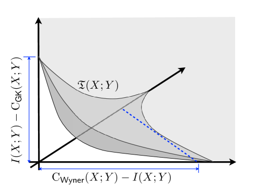
Figure 2: A schematic representation of the region $\mathfrak{T}({X};{Y})$. $\mathfrak{T}({X};{Y})$ is an unbounded, convex region, bounded away from the origin (unless $(X,Y)$ is perfectly resolvable). Relationship between two points on the boundary of $\mathfrak{T}({X};{Y})$ and the quantities ${\mathrm{C}}_{\text{\sf$\text{\sf GK}$}}$ (X;Y) and ${\mathrm{C}}_{\text{\sf$\sf Wyner$}}$ (X;Y) (see (16) and (33)) is shown. (The dotted line is at 45^∘ to the axes.)

We point out that $\mathfrak{T}({X};{Y})$ intersects all three axes (e.g., consider $Q=Y$, $Q=X$ and $Q=0$, respectively). It will be of interest to consider the three axes intercepts of the boundary of $\mathfrak{T}({X};{Y})$.

$$\begin{split}T^{\mathrm{int}}_{1}({X};{Y})&\triangleq\min\{r_{1}:(r_{1},0,0)\in\mathfrak{T}({X};{Y})\}\\ T^{\mathrm{int}}_{2}({X};{Y})&\triangleq\min\{r_{2}:(0,r_{2},0)\in\mathfrak{T}({X};{Y})\}\\ T^{\mathrm{int}}_{3}({X};{Y})&\triangleq\min\{r_{3}:(0,0,r_{3})\in\mathfrak{T}({X};{Y})\}\end{split}$$ (4)

The use of $\min$ instead of $\inf$ anticipates Theorem II.4 which shows that $\mathfrak{T}({X};{Y})$ is closed.

II-B Some Properties of Tension

Firstly, we have an easy observation.

Theorem II.1

$\mathfrak{T}({X};{Y})$ includes the origin if and only if the pair $(X,Y)$ is perfectly resolvable.

Proof:

We need to show that there exists ${p_{Q|XY}}$ such that $I(Y;Q|X)=I(X;Q|Y)=I(X;Y|Q)=0$ if and only if there exists $p_{Q^{\prime}|XY}$ such that $H(Q^{\prime}|X)=H(Q^{\prime}|Y)=I(X;Y|Q^{\prime})=0$. Clearly, the second condition implies the first by taking $Q$ to be the same as $Q^{\prime}$. The converse follows from Lemma A.1 which shows that given ${p_{Q|XY}}$ such that $I(Y;Q|X)=I(X;Q|Y)=0$, we can find a random variable $Q^{\prime}$ with $H(Q^{\prime}|X)=H(Q^{\prime}|Y)=0$ and $Q-Q^{\prime}-XY$; then, by Lemma A.2 it follows that $I(X;Y|Q^{\prime})\leq I(X;Y|Q)$, and hence $I(X;Y|Q)=0$ implies $I(X;Y|Q^{\prime})=0$. ∎

The more interesting case is when $\mathfrak{T}({X};{Y})$ does not contain the origin, and hence $(X,Y)$ is not perfectly resolvable. Note that it is important to consider all three coordinates of $T({X};{Y}|{Q})$ together to identify the unresolvable nature of a pair $(X,Y)$, because, as observed above, $\mathfrak{T}({X};{Y})$ does intersect each of the three axes, or in other words, any two coordinates of $T({X};{Y}|{Q})$ can be made simultaneously 0 by choosing an appropriate $Q$.

As it turns out, the axes intercepts are identical to three quantities identified by Wolf and Wullschleger [30]. In [30] these quantities were defined as

$$H(X\searrow Y|Y) H(Y\searrow X|X) I(X;Y|X\wedge Y)$$

where, $X\searrow Y$ stands for the part of $X$ which depends on $Y$ (i.e., a function of $X$ which distinguishes between different values of $X$ if and only if they induce different conditional distributions on $Y$), and $X\wedge Y$ stands for the common information between $X$ and $Y$ (i.e., the ”maximal” function of $X$ that is also a function of $Y$, as discussed in more detail in Section III). More precisely, the three quantities considered there are such that:

$$H(Y\searrow X|X) =\min_{{p_{Q|XY}}:H(Q|Y)=I(X;Y|Q)=0}H(Q|X)$$

$$H(X\searrow Y|Y) =\min_{{p_{Q|XY}}:H(Q|X)=I(X;Y|Q)=0}H(Q|Y)$$

$$I(X;Y|X\wedge Y) =\min_{{p_{Q|XY}}:H(Q|X)=H(Q|Y)=0}I(X;Y|Q).$$

In the appendix we prove the following theorem that these three quantities are the same as $(T^{\mathrm{int}}_{1}({X};{Y}),T^{\mathrm{int}}_{2}({X};{Y}),T^{\mathrm{int}}_{3}({X};{Y}))$.

Theorem II.2

$$T^{\mathrm{int}}_{1}({X};{Y}) =\min_{\begin{subarray}{c}{p_{Q|XY}}:\\ H(Q|Y)=I(X;Y|Q)=0\end{subarray}}H(Q|X)$$ (5)

$$T^{\mathrm{int}}_{2}({X};{Y}) =\min_{\begin{subarray}{c}{p_{Q|XY}}:\\ H(Q|X)=I(X;Y|Q)=0\end{subarray}}H(Q|Y)$$ (6)

$$T^{\mathrm{int}}_{3}({X};{Y}) =\min_{\begin{subarray}{c}{p_{Q|XY}}:\\ H(Q|X)=H(Q|Y)=0\end{subarray}}I(X;Y|Q).$$ (7)

Monotonicity of $\mathfrak{T}({X};{Y})$

Wolf and Wullschleger showed that these three quantities have a certain “monotonicity” property (they can only decrease, as $X,Y$ evolve as the views of two parties in a secure protocol). We shall see that the monotinicity of all the three quantities is a consequence of the monotinicity of the entire region $\mathfrak{T}({X};{Y})$. We define the precise nature of this monotonicity in Section V-B and prove it for $\mathfrak{T}({X};{Y})$ in Section V-C.

The following result (proven in Appendix A) will be useful in defining a “multiplication” operation on the region of tension as a scaling (see (43)). This in turn would be useful in relating the region of tension and the rate of secure sampling, in Section V.

Theorem II.3

The region $\mathfrak{T}({X};{Y})$ is convex.

In extending the results in Section V to statistical security (rather than perfect security), the following results would be important. Firstly, the region of tension is closed.

Theorem II.4

The region $\mathfrak{T}({X};{Y})$ is closed.

Proof:

By (3), and the fact that the increasing hull of a compact set is closed (see Lemma A.3 in Appendix A), it is enough to show that $\{T({X};{Y}|{Q}):{p_{Q|XY}}\in\widehat{}{\mathcal{P}}_{X,Y}\}$ is compact (i.e., closed and bounded (Heine-Borel theorem)). For this, notice that $T({X};{Y}|{Q})$ as a function of $p_{Q|XY}$ – i.e., as a function from $\widehat{}{\mathcal{P}}_{X,Y}$ to $\mathbb{R}^{3}$ – is continuous. Moreover, $\widehat{}{\mathcal{P}}_{X,Y}$ is compact. Since the image of a compact set under a continuous function is compact, $\{T({X};{Y}|{Q}):{p_{Q|XY}}\in\widehat{}{\mathcal{P}}_{X,Y}\}$ is compact. ∎

Secondly, the region of tension is continuous in the sense that when the joint p.m.f. $p_{X,Y}$ is close to the joint p.m.f. $p_{X^{\prime},Y^{\prime}}$, the tension regions $\mathfrak{T}({X};{Y})$ and $\mathfrak{T}({X^{\prime}};{Y^{\prime}})$ are also close. We measure closeness of these two joint p.m.f.’s (assumed without loss of general to be defined over the same alphabet $\mathcal{X}\times\mathcal{Y}$) by their total variation distance $\Delta(XY,X^{\prime}Y^{\prime})$.

Theorem II.5

Suppose $\Delta(XY,X^{\prime}Y^{\prime})=\epsilon$, for some $\epsilon\in[0,1]$. Then, $\mathfrak{T}({X};{Y})\subseteq\mathfrak{T}({X^{\prime}};{Y^{\prime}})-\delta(\epsilon)$, where $\delta(\epsilon)=2H_{2}(\epsilon)+\epsilon\log\max\{|\mathcal{X}|,|\mathcal{Y}|\}$, and for ${\sf S}\in\mathbb{R}^{3},\alpha\in\mathbb{R}$, the notation ${\sf S}-\alpha$ stands for $\{(r_{1}-\alpha,r_{2}-\alpha,r_{3}-\alpha):(r_{1},r_{2},r_{3})\in{\sf S}\}$.

Proof:

Suppose $(r_{1},r_{2},r_{3})\in\mathfrak{T}({X};{Y})$. We shall show that $(r_{1}+\delta(\epsilon),r_{2}+\delta(\epsilon),r_{3}+\delta(\epsilon))\in\mathfrak{T}({X^{\prime}};{Y^{\prime}})$. Since $(r_{1},r_{2},r_{3})\in\mathfrak{T}({X};{Y})$, there is a $p_{Q|X,Y}\in{\mathcal{P}}_{X,Y}$ such that $I(Y;Q|X)\leq r_{1}$, $I(X;Q|Y)\leq r_{2}$, and $I(X;Y|Q)\leq r_{3}$. Let $p_{Q^{\prime}|X^{\prime},Y^{\prime}}=p_{Q|X,Y}$. It is enough to prove that

$$I(Y^{\prime};Q^{\prime}|X^{\prime}) \leq I(Y;Q|X)+\delta(\epsilon),$$

$$I(X^{\prime};Q^{\prime}|Y^{\prime}) \leq I(X;Q|Y)+\delta(\epsilon),$$

$$I(X^{\prime};Y^{\prime}|Q^{\prime}) \leq I(X;Y|Q)+\delta(\epsilon).$$

We will make use of the following lemma which is proved in Appendix A.

Lemma II.6

Suppose random variables $(A,B,C)$ and $(A^{\prime},B^{\prime},C^{\prime})$ over the same alphabet $\mathcal{A}\times\mathcal{B}\times\mathcal{C}$ are such that $\Delta(ABC,A^{\prime}B^{\prime}C^{\prime})=\epsilon$. Then $I(A^{\prime};B^{\prime}|C^{\prime})\leq I(A;B|C)+2H_{2}(\epsilon)+\epsilon\log\min\{|\mathcal{A}|,|\mathcal{B}|\}$.

Note that since $p_{Q^{\prime}|X^{\prime},Y^{\prime}}=p_{Q|X,Y}$, we have $\Delta(XYQ,X^{\prime}Y^{\prime}Q^{\prime})=\Delta(XY,X^{\prime}Y^{\prime})=\epsilon$. Then we invoke Lemma II.6 thrice (with $(ABC,A^{\prime}B^{\prime}C^{\prime})$ standing for $(YQX,Y^{\prime}Q^{\prime}X^{\prime})$, $(XQY,X^{\prime}Q^{\prime}Y^{\prime})$ and $(XYQ,X^{\prime}Y^{\prime}Q^{\prime})$, respectively). This combined with the fact that $\min\{|\mathcal{Y}|,|\mathcal{Q}|\}$, $\min\{|\mathcal{X}|,|\mathcal{Q}|\}$, $\min\{|\mathcal{X}|,|\mathcal{Y}|\}$, are all upperbounded by $\max\{|\mathcal{X}|,|\mathcal{Y}|\}$, we obtain the requisite bounds.

∎

II-C A Few Examples

Obtaining closed form expressions for the region $\mathfrak{T}({X};{Y})$ can be difficult. However, for our applications it often suffices to identify parts of the boundary of $\mathfrak{T}({X};{Y})$. We give a couple of examples below. A more detailed example appears in Section V-E.

Example II.1

Figure 3 shows the joint p.m.f. of a pair of dependent random variables $X,Y$.

Figure 3: $X,Y$ are dependent random variables whose joint p.m.f is shown on the left. The solid black lines each carry a probability mass of $\frac{1-\delta}{8}$ and the lighter ones $\frac{\delta}{8}$. In the plot, all points $(R_{1},R_{2})$ on the dotted lines are such that $(R_{1},R_{2},0)\in\mathfrak{T}({X};{Y})$.

When $\delta=0$, they have the simple dependency structure of $X=(X^{\prime},Q),Y=(Y^{\prime},Q)$ where $X^{\prime},Y^{\prime},Q$ are independent. This is the perfectly resolvable case. Thus, the set of rate pairs $(R_{1},R_{2})$ such that $(R_{1},R_{2},0)\in\mathfrak{T}({X};{Y})$ is the entire positive quadrant. For small values of $\delta$ we intuitively expect the random variables to be “close” to this case. A measure such as the common information of Gács and Körner fails to bring this out (common information is discontinuous in $\delta$ jumping from $H(Q)=1$ at $\delta=0$ to 0 for $\delta>0$). However, the intuition is borne out by our trade-off regions. For instance, for $\delta=0.05$, Figure 3 shows that the set of rate pairs $(R_{1},R_{2})$ such that $(R_{1},R_{2},0)\in\mathfrak{T}({X};{Y})$ is nearly all of the positive quadrant.

Example II.2

A binary example. Figure 4 shows the joint p.m.f. of a pair of dependent binary random variables $U,V$. In the plot in Figure 4 we show the intersection of $\mathfrak{T}({U};{V})$ with the plane $z=0$. The computation is along the lines of Section V-E.

Figure 4: $U,V$ are binary random variables with joint p.m.f. $p(0,0)=p(1,1)=p$, $p(1,0)=1-2p$, and $p(0,1)=0$. The plot shows the boundary of the set of all rate pairs $(R_{1},R_{2})$ such that $(R_{1},R_{2},0)\in\mathfrak{T}({U};{V})$ for three values of $p$. When $p$ approaches 0 or $0.5$, this boundary approaches the axes, indicating that the random variables are closer to being perfectly resolvable.

III Assisted Common Information

Recall that when $X=(X^{\prime},Q)$ and $Y=(Y^{\prime},Q)$ where $X^{\prime},Y^{\prime},Q$ are independent, then a natural measure of “common information” of $X$ and $Y$ is $H(Q)$. In this case, an observer of $X$ and an observer of $Y$ may independently produce the common part $Q$; and conditioned on $Q$, there is no “residual information” that correlates $X$ and $Y$ i.e., $I(X;Y|Q)=0$. The definition ${\mathrm{C}}_{\text{\sf$\text{\sf GK}$}}(X;Y)$ of Gács and Körner [9] generalizes this to arbitrary $X,Y$ (Figure 5(a)): the two observers now see $X^{n}=(X_{1},\ldots,X_{n})$ and $Y^{n}=(Y_{1},\ldots,Y_{n})$, resp., where $(X_{i},Y_{i})$ pairs are independent drawings of $(X,Y)$. They are required to produce random variables $W_{1}=f_{1}(X^{n})$ and $W_{2}=f_{2}(Y^{n})$, resp., which agree (with high probability). The largest entropy rate (i.e., entropy normalized by $n$) of such a “common” random variable was proposed as the common information of $X$ and $Y$. We will refer to this as the GK common information of $(X,Y)$ and denote it by ${\mathrm{C}}_{\text{\sf$\text{\sf GK}$}}(X;Y)$. However, in the same paper [9], Gács and Körner showed (a result later strengthened by Witsenhausen [28]) that this rate is still just the largest $H(Q)$ for $Q$ which can be obtained (with probability 1) as a deterministic function of $X$ alone as well as a deterministic function of $Y$ alone.

$${\mathrm{C}}_{\text{\sf$\text{\sf GK}$}}(X;Y)=\max_{\begin{subarray}{c}{p_{Q|XY}}:\\ H(Q|X)=H(Q|Y)=0\end{subarray}}H(Q).$$

It is easy to see that the above maximum is achieved by the random variable $Q$ defined over the set of connected components of the characteristic bipartite graph of $(X,Y)$, such that $p_{Q|XY}(q|x,y)=1$ if and only if the edge $(x,y)$ belongs to the connected component $q$. Note that this captures only an explicit form of common information in a single instance of $(X,Y)$.

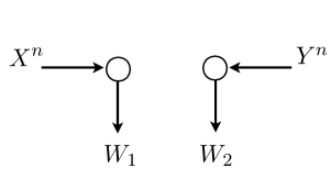
(a)

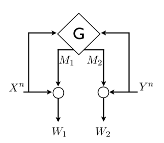
(b)

Figure 5: (a) Setup for Gács-Körner common information. The observers generate $W_{1}$ and $W_{2}$ which are required to agree with high probability. (b) Assisted common information system. A genie assists the observers by sending separate messages to them over rate-limited noiseless links. When the genie is absent the setup reduces to the one for Gács-Körner common information.

One limitation of the common information defined by Gács and Körner is that it ignores information which is almost common. In particular, if there is only a single connected component in the characteristic bipartite graph then the common information between them is zero, even if it is the case that by removing a set of edges that account for a small probability mass, the graph can be disconnected into a large number of components each with a significant probability mass. Our approach in this section could be viewed as a strict generalization of Gács and Körner, which uncovers such extra layers of “almost common information.” Technically, we introduce an omniscient genie who has access to both the observations $X^{n}$ and $Y^{n}$ and can send separate messages to the two observers over rate-limited noiseless links. See Figure 5(b). The objective is for the observers to agree on a “common” random variable as before, but now with the genie’s assistance. We call this the assisted common information system. This leads to a trade-off region trading-off the rates of the noiseless links and the resulting common information (or the resulting residual mutual information). We characterize these trade-off regions in terms of the region of tension of the two random variables, and show that, in general, they exhibit non-trivial behavior, but reduce to the trivial behaviour discussed above when the rates of the noiseless links are zero.

As before, two observers receive $X^{n}=(X_{1},\dotsc,X_{n})$ and $Y^{n}=(Y_{1},\dotsc,Y_{n})$ respectively, and need to output strings $W_{1}$ and $W_{2}$ respectively, that must match each other with high probability. But here, an omniscient Genie $G$ computes $M_{1}=f_{1}^{(n)}(X^{n},Y^{n})$ and $M_{2}=f_{2}^{(n)}(X^{n},Y^{n})$ as deterministic functions of $(X^{n},Y^{n})$ and sends these to the two observers as shown in Figure 5(b). The observers are allowed to compute their outputs also making use of the respective messages they receive from the genie, as $W_{1}=g_{1}^{(n)}(X^{n},M_{1})$ and $W_{2}=g_{2}^{(n)}(Y^{n},M_{2})$, where $g_{1}^{(n)}$ and $g_{2}^{(n)}$ are deterministic functions. Here again, the goal is to study how large the entropy of $W_{1}$ (and equivalently $W_{2}$) can be, but controlling for the number of bits used to transmit $M_{1}$ and $M_{2}$.

For a pair of random variables $(X,Y)$ and positive integers $N_{1},N_{2},n$, an $(N_{1},N_{2},n)$ assisted common information (ACI) code is defined as a quadruple $(f_{1}^{(n)},f_{2}^{(n)},g_{1}^{(n)},g_{2}^{(n)})$, where

$$f_{k}^{(n)} :\mathcal{X}^{n}\times\mathcal{Y}^{n}\rightarrow\{1,\ldots,N_{k}\},\quad k=1,2$$

$$g_{1}^{(n)} :\mathcal{X}^{n}\times\{1,\ldots,N_{1}\}\rightarrow\mathbb{Z},\text{ and}$$

$$g_{2}^{(n)} :\mathcal{Y}^{n}\times\{1,\ldots,N_{2}\}\rightarrow\mathbb{Z}$$

are deterministic functions. A sequence of $(N_{1}(n),N_{2}(n),n)$ ACI codes $(f_{1}^{(n)},f_{2}^{(n)},g_{1}^{(n)},g_{2}^{(n)})_{n=1,2,\ldots}$ is called a valid $(R_{1},R_{2})$ ACI strategy for $(X,Y)$, if for every $\epsilon>0$, for sufficiently large $n$,

$$\frac{1}{n}\log N_{k}(n) \leq R_{k}+\epsilon,\quad k=1,2$$ (8)

$$\Pr[g_{1}^{(n)}(X^{n},f_{1}^{(n)}(X^{n},Y^{n})) \neq g_{2}^{(n)}(Y^{n},f_{2}^{(n)}(X^{n},Y^{n}))]$$

$$\qquad\qquad\qquad\leq\epsilon.$$ (9)

We say that a rate pair $(R_{1},R_{2})$ enables common information rate $R_{\text{\sf CI}}\geq 0$ for $(X,Y)$, if there exists a valid $(R_{1},R_{2})$ ACI strategy ${(f_{1}^{(n)},f_{2}^{(n)},g_{1}^{(n)},g_{2}^{(n)})}_{n}$ for $(X,Y)$ such that for every $\epsilon>0$, for sufficiently large $n$,

$$\frac{1}{n}H(g_{1}^{(n)}(X^{n},f_{1}^{(n)}(X^{n},Y^{n})))\geq R_{\text{\sf CI}}-\epsilon.$$ (10)

Similarly, we say that a rate pair $(R_{1},R_{2})$ enables residual information rate $R_{\text{\sf RI}}$ for $(X,Y)$, if there exists a valid $(R_{1},R_{2})$ ACI strategy $(f_{1}^{(n)},f_{2}^{(n)},g_{1}^{(n)},g_{2}^{(n)})_{n}$ for $(X,Y)$ such that for every $\epsilon>0$, for sufficiently large $n$,

$$\frac{1}{n}I(X^{n};Y^{n}|g_{1}^{(n)}(X^{n},f_{1}^{(n)}(X^{n},Y^{n}))) \leq R_{\text{\sf RI}}+\epsilon.$$ (11)

Note that if $(R_{1},R_{2})$ enables residual information rate $R_{\text{\sf RI}}$, and $(R_{1}^{\prime},R_{2}^{\prime},R_{\text{\sf RI}}^{\prime})\geq(R_{1},R_{2},R_{\text{\sf RI}})$, then $(R_{1}^{\prime},R_{2}^{\prime})$ enables residual information rate $R_{\text{\sf RI}}^{\prime}$ too.

Definition III.1

The assisted common information region ${\mathcal{R}}_{\text{\sf ACI}}(X;Y)$ of a pair of correlated random variables $(X,Y)$ is the set of all $(R_{1},R_{2},R_{\text{\sf CI}})\in{\mathbb{R}}_{+}^{3}$ such that $(R_{1},R_{2})$ enables common information rate $R_{\text{\sf CI}}$ for $(X,Y)$. Similarly the assisted residual information rate region ${\mathcal{R}}_{\text{\sf ARI}}(X;Y)$ of $(X,Y)$ is the set of all $(R_{1},R_{2},R_{\text{\sf RI}})\in{\mathbb{R}}_{+}^{3}$ such that $(R_{1},R_{2})$ enables residual information rate $R_{\text{\sf RI}}$ for $(X,Y)$. In other words,

$${\mathcal{R}}_{\text{\sf ACI}}(X;Y) \triangleq\{(R_{1},R_{2},R_{\text{\sf CI}}):(R_{1},R_{2})\text{ enables }$$

$$\text{common information rate }R_{\text{\sf CI}}\text{ for }(X,Y)\},$$

$${\mathcal{R}}_{\text{\sf ARI}}(X;Y) \triangleq\{(R_{1},R_{2},R_{\text{\sf RI}}):(R_{1},R_{2})\text{ enables }$$

$$\text{residual information rate }R_{\text{\sf RI}}\text{ for }(X,Y)\}.$$

We will write ${\mathcal{R}}_{\text{\sf ACI}}$ and ${\mathcal{R}}_{\text{\sf ARI}}$ when the random variables involved are obvious from the context. It is easy to see from the definition that ${\mathcal{R}}_{\text{\sf ACI}}$ and ${\mathcal{R}}_{\text{\sf ARI}}$ are closed sets.

Our main results regarding assisted common information system characterize the assisted residual and common information rate regions of $(X,Y)$, and relate them to the region of tension of $(X,Y)$.

Recall that $\widehat{}{\mathcal{P}}_{X,Y}$ is the set of all conditional p.m.f.’s $p_{Q|X,Y}$ such that the cardinality of alphabet $\mathcal{Q}$ of $Q$ is such that $|\mathcal{Q}|\leq|\mathcal{X}||\mathcal{Y}|+2$. We have the following characterization of the assisted common and residual information regions:

Theorem III.1

$${\mathcal{R}}_{\text{\sf ARI}}(X;Y)=\{(r_{1},r_{2},r_{\text{\sf RI}})\in{\mathbb{R}}_{+}^{3}:\exists{p_{Q|XY}}\in\widehat{}{\mathcal{P}}_{X,Y}\text{ s.t.}$$

$$\;\;\;\;r_{1}\geq I(Y;Q|X),r_{2}\geq I(X;Q|Y),r_{\text{\sf RI}}\geq I(X;Y|Q)\}.$$

$${\mathcal{R}}_{\text{\sf ACI}}(X;Y)=\{(r_{1},r_{2},r_{\text{\sf CI}})\in{\mathbb{R}}_{+}^{3}:\exists{p_{Q|XY}}\in\widehat{}{\mathcal{P}}_{X,Y}\text{ s.t.}$$

$$\;\;\;\;r_{1}\geq I(Y;Q|X),r_{2}\geq I(X;Q|Y),r_{\text{\sf CI}}\leq I(X,Y;Q)\}.$$

We prove this theorem in Section III-B. An immediate consequence is that we have an interpretation of the region of tension $\mathfrak{T}({X};{Y})$ as the assisted residual information region ${\mathcal{R}}_{\text{\sf ARI}}(X;Y)$. We may also write it down in terms of the assisted common information region:

Corollary III.2

For any pair of correlated random variables $(X,Y)$,

$$\mathfrak{T}({X};{Y}) ={\mathcal{R}}_{\text{\sf ARI}}(X;Y)$$ (12)

$$\mathfrak{T}({X};{Y}) =i\left(f_{X,Y}({\mathcal{R}}_{\text{\sf ACI}}(X;Y))\right)$$ (13)

where $f_{X,Y}$ is an affine map defined as

$$f_{X,Y}\left(\left[\begin{array}[]{c}R_{1}\\ R_{2}\\ R_{3}\end{array}\right]\right)\triangleq\left[\begin{array}[]{c}R_{1}\\ R_{2}\\ I(X;Y)+R_{1}+R_{2}-R_{3}\end{array}\right].$$

We prove (13) in Appendix B.

III-A Behavior at $R_{1}=R_{2}=0$ and Connection to Gács-Körner [9]

As discussed above, Gács and Körner defined the common information, ${\mathrm{C}}_{\text{\sf$\text{\sf GK}$}}(X;Y)$ using the system in Figure 5(a), where there is no genie. Formally, an $n$-GK map-pair $(g_{1}^{(n)},g_{2}^{(n)})$ is a pair of maps $g_{1}^{(n)}:\mathcal{X}^{n}\rightarrow\mathbb{Z}$ and $g_{2}^{(n)}:\mathcal{Y}^{n}\rightarrow\mathbb{Z}$. We will say that $R_{\text{\sf CI}}$ is an achievable common information rate for $(X,Y)$ if there is a sequence of GK map-pairs $(g_{1}^{(n)},g_{2}^{(n)})_{n=1,2,\ldots}$ such that for every $\epsilon>0$, for large enough $n$,

$$\Pr[g_{1}^{(n)}(X^{n})\neq g_{2}^{(n)}(Y^{n})] \leq\epsilon,\text{ and}$$

$$\frac{1}{n}H\left(g_{1}^{(n)}(X^{n})\right) \geq R_{\text{\sf CI}}-\epsilon.$$

GK common information ${\mathrm{C}}_{\text{\sf$\text{\sf GK}$}}(X;Y)$ is the supremum of all achievable common infomation rates for $(X,Y)$. As mentioned earlier, Gács and Körner [9] showed that ${\mathrm{C}}_{\text{\sf$\text{\sf GK}$}}(X;Y)$ is simply $H(Q)$ where $Q$ corresponds to the connected component in the characteristic bipartite graph of $(X,Y)$.

It is clear from the definition that $(0,0,{\mathrm{C}}_{\text{\sf$\text{\sf GK}$}}(X;Y))\in{\mathcal{R}}_{\text{\sf ACI}}(X;Y)$. However, it is not clear whether ${\mathrm{C}}_{\text{\sf$\text{\sf GK}$}}(X;Y)$ is the largest value of $R_{\text{\sf CI}}$ such that $(0,0,R_{\text{\sf CI}})\in{\mathcal{R}}_{\text{\sf ACI}}(X;Y)$; i.e., if we define ${{\mathcal{R}}_{\text{\sf ACI}}}_{,3}^{\mathrm{int}}({X};{Y})$ as the axis intercept of the boundary of ${\mathcal{R}}_{\text{\sf ACI}}(X;Y)$ along the $R_{\text{\sf CI}}$ axis as follows

$${{\mathcal{R}}_{\text{\sf ACI}}}_{,3}^{\mathrm{int}}({X};{Y}) \triangleq\max\{R_{\text{\sf CI}}:(0,0,R_{\text{\sf CI}})\in{\mathcal{R}}_{\text{\sf ACI}}(X;Y)\},$$

then it is not immediately clear whether ${\mathrm{C}}_{\text{\sf$\text{\sf GK}$}}(X;Y)={{\mathcal{R}}_{\text{\sf ACI}}}_{,3}^{\mathrm{int}}({X};{Y})$. This is because the absence of links from the genie is a more restrictive condition than allowing “zero-rate” links from the genie (notice the $\epsilon$ in (8)). So we may ask whether introducing an omniscient genie, but with zero-rate links to the observers, changes the conclusion of Gács-Körner. In other words, whether ${{\mathcal{R}}_{\text{\sf ACI}}}_{,3}^{\mathrm{int}}({X};{Y})$ is larger than ${\mathrm{C}}_{\text{\sf$\text{\sf GK}$}}(X;Y)$. The corollary below (proven in Appendix B) answers this question in the negative. Also note that the result of Gács-Körner can be obtained as a simple consequence of this corollary.

Corollary III.3

$${\mathrm{C}}_{\text{\sf$\text{\sf GK}$}}(X;Y) ={{\mathcal{R}}_{\text{\sf ACI}}}_{,3}^{\mathrm{int}}({X};{Y})$$ (14)

$$=\max_{\begin{subarray}{c}{p_{Q|XY}}\in{\mathcal{P}}_{X,Y}:\\ H(Q|X)=H(Q|Y)=0\end{subarray}}H(Q).$$ (15)

Further,

$$T^{\mathrm{int}}_{3}({X};{Y}) =I(X;Y)-{\mathrm{C}}_{\text{\sf$\text{\sf GK}$}}(X;Y)$$ (16)

Thus, at zero rates for the links, assisted common information exhibits the same trivial behavior as ${\mathrm{C}}_{\text{\sf$\text{\sf GK}$}}$.

III-B Proof of Theorem III.1

We first prove the converse (i.e., $\text{L.H.S.}\subseteq\text{R.H.S.}$). Let $\epsilon>0$, and $n$ and an $(N_{1}(n),N_{2}(n),n)$ ACI code $(f_{1}^{(n)},f_{2}^{(n)},g_{1}^{(n)},g_{2}^{(n)})$ be such that (8)-(10) hold. Let $C_{k}=f_{k}^{(n)}(X^{n},Y^{n})$, for $k=1,2$, and $W_{1}=g_{1}^{(n)}(X^{n},C_{1})$ and $W_{2}=g_{2}^{(n)}(Y^{n},C_{2})$. Then,

$$R_{1}+\epsilon \geq\frac{1}{n}H(C_{1})\geq\frac{1}{n}H(C_{1}|X^{n})\geq\frac{1}{n}H(W_{1}|X^{n})$$

$$\geq\frac{1}{n}I(Y^{n};W_{1}|X^{n})$$

$$\stackrel{{\scriptstyle\mathrm{(a)}}}{{=}}\frac{1}{n}\sum_{i=1}^{n}H(Y_{i}|X_{i})-H(Y_{i}|Y^{i-1},X^{n},W_{1})$$

$$\geq\frac{1}{n}\sum_{i=1}^{n}H(Y_{i}|X_{i})-H(Y_{i}|X_{i},W_{1},Y^{i-1},X^{i-1})$$

$$=\sum_{i=1}^{n}\frac{1}{n}I(Y_{i};Q_{i}|X_{i}),$$

$$\qquad\qquad\qquad\text{ }Q_{i}\triangleq(W_{1},Y^{i-1},X^{i-1})$$

$$\stackrel{{\scriptstyle\mathrm{(b)}}}{{=}}I(Y_{J};Q_{J}|X_{J},J),$$

$$\qquad\qquad\qquad\text{ }p_{J}(i)\triangleq\frac{1}{n},i\in\{1,\dotsc,n\},$$

$$\stackrel{{\scriptstyle\mathrm{(c)}}}{{=}}I(Y_{J};Q|X_{J}),\qquad\qquad\text{ }Q\triangleq(Q_{J},J),$$

where (a) follows from the independence of $(X_{i},Y_{i})$ pairs across $i$. In (b), we define $J$ to be a random variable uniformly distributed over $\{1,\ldots,n\}$ and independent of $(X^{n},Y^{n})$. And (c) follows from the independence of $J$ and $(X^{n},Y^{n})$. Similarly,

$$R_{2}+\epsilon \geq\frac{1}{n}H(C_{2}|Y^{n})\geq\frac{1}{n}H(W_{2}|Y^{n})$$

$$=\frac{1}{n}H(W_{1},W_{2}|Y^{n})-\frac{1}{n}H(W_{1}|W_{2},Y^{n})$$

$$\geq\frac{1}{n}H(W_{1}|Y^{n})-\frac{1}{n}H(W_{1}|W_{2})$$

$$\stackrel{{\scriptstyle\mathrm{(a)}}}{{\geq}}H(W_{1}|Y^{n})-\kappa\epsilon$$

$$\geq\frac{1}{n}I(X^{n};W_{1}|Y^{n})-\kappa\epsilon$$ (17)

$$\stackrel{{\scriptstyle\mathrm{(b)}}}{{\geq}}I(X_{J};Q|Y_{J})-\kappa\epsilon,$$

where (a) (with $\kappa\triangleq 1+\log|\mathcal{X}||\mathcal{Y}|$) follows from Fano’s inequality and the fact that the range of $g_{1}$ can be restricted without loss of generality to a set of cardinality $|\mathcal{X}|^{n}|\mathcal{Y}|^{n}$. And (b) can be shown along the same lines as the chain of inequalities which gave a lower bound for $R_{1}$ above. Moreover,

$$\frac{1}{n}I(X^{n};Y^{n}|W_{1}) =\frac{1}{n}\sum_{i=1}^{n}I(X_{i};Y^{n}|W_{1},X^{i-1})$$

$$\geq\frac{1}{n}\sum_{i=1}^{n}I(X_{i};Y_{i}|W_{1},X^{i-1},Y^{i-1})$$

$$=I(X_{J};Y_{J}|Q).$$

Since $X_{J},Y_{J}$ has the same joint distribution as $X,Y$, the converse for assisted residual information follows. Similarly, the converse for assisted common information can be shown using

$$\frac{1}{n}H(W_{1})$$

$$\qquad\stackrel{{\scriptstyle\mathrm{(a)}}}{{=}}\frac{1}{n}I(X^{n},Y^{n};W_{1})$$

$$\qquad=\frac{1}{n}\sum_{i=1}^{n}H(X_{i},Y_{i})-H(X_{i},Y_{i}|W_{1},X^{i-1},Y^{i-1})$$

$$\qquad=\frac{1}{n}\sum_{i=1}^{n}I(X_{i},Y_{i};Q_{i})=I(X_{J},Y_{J};Q),$$

where (a) follows from the fact that $W_{1}$ is a deterministic function of $(X^{n},Y^{n})$. The fact that instead of ${p_{Q|XY}}\in{\mathcal{P}}_{X,Y}$ we can consider ${p_{Q|XY}}\in\widehat{}{\mathcal{P}}_{X,Y}$ with alphabet $\mathcal{Q}$ such that $|\mathcal{Q}|\leq|\mathcal{X}||\mathcal{Y}|+2$ follows from Fenchel-Eggleston’s strengthening of Carathéodory’s theorem [6, pg. 310].

To prove achievability (i.e., $\text{L.H.S.}\supseteq\text{R.H.S.}$), we will use a result from lossy source coding. See, e.g., [4, Chapter 10] for a description of the lossy source coding problem. Consider a source $p_{S}$, and source and reconstruction alphabets $\mathcal{S}$ and $\widehat{\mathcal{S}}$, respectively. We have the following lemma:

Lemma III.4

Given a conditional distribution $p^{\ast}_{\widehat{S}|S}$, there is a distortion measure $d:\mathcal{S}\times\widehat{\mathcal{S}}\rightarrow{\mathbb{R}}_{+}\cup\{\infty\}$, and a distortion constraint $D$ such that the $p^{\ast}_{\widehat{S}|S}$ is a minimizer for

$$R(D)=\min_{p_{\widehat{S}|S}:{\mathbb{E}}_{p_{S\vphantom{\widehat{S}}}p_{\widehat{S}|S}}\left[d(S,\widehat{S})\right]\leq D}I(S;\widehat{S}).$$

Moreover, unless $I(S;\widehat{S})=0$ (in which case any $d$ works), the distortion measure $d$ is given by

$$d(s,\hat{s}) =-c\log p^{\ast}_{S|\widehat{S}}(s|\hat{s})+d_{0}(s),$$ (18)

where $$c>0 d_{0}$$ and the function can be chosen arbitrarily, and

$$p^{\ast}_{S|\widehat{S}}(s|\hat{s}) =\frac{p^{\vphantom{\ast}}_{S\vphantom{\widehat{S}}}(s)p^{\ast}_{\widehat{S}|S}(\hat{s}|s)}{\sum_{\tilde{s}}p^{\vphantom{\ast}}_{S\vphantom{\widehat{S}}}(\tilde{s})p^{\ast}_{\widehat{S}|S}(\hat{s}|\tilde{s})}.$$

The distortion constraint $D$ is given by

$$D ={\mathbb{E}}_{p^{\vphantom{\ast}}_{S\vphantom{\widehat{S}}}p^{\ast}_{\widehat{S}|S}}\left[d(S,\widehat{S})\right]$$

Proof:

See [6, Problem 3, pg. 147]; also see [10, Lemma 4] for a proof. ∎

For a given $p^{\ast}_{Q|XY}\in\widehat{}{\mathcal{P}}_{X,Y}$, we need to argue that

$$(I(Y;Q|X),I(X;Q|Y),I(X,Y;Q)) \in{\mathcal{R}}_{\text{\sf ACI}}(X;Y),$$

$$(I(Y;Q|X),I(X;Q|Y),I(X;Y|Q)) \in{\mathcal{R}}_{\text{\sf ARI}}(X;Y),$$

where the conditional mutual information quantities are evaluated using the joint distribution $p^{\vphantom{\ast}}_{X,Y}p^{\ast}_{Q|XY}$. Note that these quantities are continuous in $p^{\ast}_{Q|XY}$. Moreover, as was mentioned earlier, it is easy to verify from their definitions that ${\mathcal{R}}_{\text{\sf ACI}}(X;Y)$ and ${\mathcal{R}}_{\text{\sf ARI}}(X;Y)$ are closed sets. Hence, we may make the following assumption on $p^{\ast}_{Q|XY}$ without loss of generality:
Assumption: $p^{\ast}_{Q|XY}(q|x,y)>0$ for all $(x,y,q)\in\mathcal{X}\times\mathcal{Y}\times\mathcal{Q}$.
In Lemma III.4, let $p^{\vphantom{\ast}}_{S}$ be $p^{\vphantom{\ast}}_{X,Y}$ and $p^{\ast}_{\widehat{S}|S}$ be $p^{\ast}_{Q|XY}$. Let $d:\mathcal{X}\times\mathcal{Y}\times\mathcal{Q}\rightarrow{\mathbb{R}}_{+}\cup\{\infty\}$ denote the distortion measure and $D^{\ast}$ the distortion constraint promised by the lemma. Let

$$d_{\mathrm{max}}=\max_{\begin{subarray}{c}(x,y)\in\mathcal{X}\times\mathcal{Y}:\\ p_{X,Y}(x,y)>0\end{subarray}}\max_{q\in\mathcal{Q}}\;d(x,y,q).$$

Under the above Assumption, it is clear from (18) that $d_{\mathrm{max}}<\infty$.

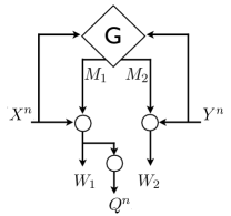
Figure 6: Set up in the proof of Theorem III.1

The rest of the proof proceeds as follows: we will define a distributed source coding problem (see Figure 6) where the first goal is for the observers to agree on a common random variable as in the assisted common information setup. However, instead of this common random variable meeting (10) or (11), we will require that an output sequence $Q^{n}$, which is produced as a deterministic function of the common random variable, must meet a distortion criterion. The distortion measure and the distortion constraint are those obtained above using Lemma III.4. We will show that these requirements can be met using a code which operates at $(R_{1},R_{2})=(I(Y;Q|X),I(X;Q|Y))$. We will then argue that this must imply that the common random variable also meets (10) and (11).

We make the following definitions (see Figure 6): we define an $(N,N_{1},N_{2},n)$ code as a quintuple $(f_{1}^{(n)},f_{2}^{(n)},g_{1}^{(n)},g_{2}^{(n)},h)$, where

$$f_{k}^{(n)} :\mathcal{X}^{n}\times\mathcal{Y}^{n}\rightarrow\{1,\ldots,N_{k}\},\quad k=1,2$$

$$g_{1}^{(n)} :\mathcal{X}^{n}\times\{1,\ldots,N_{1}\}\rightarrow\{1,\ldots,N\},$$

$$g_{2}^{(n)} :\mathcal{Y}^{n}\times\{1,\ldots,N_{2}\}\rightarrow\{1,\ldots,N\},\text{ and}$$

$$h^{(n)} :\{1,\ldots,N\}\rightarrow\mathcal{Q}^{n}$$

are deterministic functions. Note that embedded in this code is an $(N_{1},N_{2},n)$ ACI code. The probability of error of a code is defined as

$$P^{(n)}_{e}=\Pr[ \;g_{1}^{(n)}(X^{n},f_{1}^{(n)}(X^{n},Y^{n}))$$

$$\qquad\quad\neq g_{2}^{(n)}(Y^{n},f_{2}^{(n)}(X^{n},Y^{n}))].$$ (19)

Let

$$Q^{n}=h^{(n)}\left(g_{1}^{(n)}\left(X^{n},f_{1}^{(n)}(X^{n},Y^{n})\right)\right).$$

For $D\geq 0$, we will say that $(R_{1},R_{2},D)$ is achievable if there is a sequence of $(N(n),N_{1}(n),N_{2}(n),n)$ codes such that for every $\epsilon>0$, for sufficiently large $n$,

$$\frac{1}{n}\log N_{k}(n) \leq R_{k}+\epsilon,\quad k=1,2$$ (20)

$$P^{(n)}_{e} \leq\epsilon,$$ (21)

and the following average distortion contraint holds

$$\frac{1}{n}\sum_{i=1}^{n}{\mathbb{E}}\left[d(X_{i},Y_{i},Q_{i}) \leq D+\epsilon.$$ (22)

The rate-distortion tradeoff region $\mathcal{R}$ is the closure of the set of all achievable $(R_{1},R_{2},D)$.

The following lemma is proved in Appendix B using standard techniques from distributed source coding theory (see, for instance, [8, Chapter 11]).

Lemma III.5

$$(I(Y;Q|X),I(X;Q|Y),D^{\ast})\in\mathcal{R},$$

where the conditional mututal informations are evaluated using $p^{\vphantom{\ast}}_{X,Y}p^{\ast}_{Q|XY}$ and $D^{\ast}$ is given by (LABEL:eq:Dstar).

As mentioned above, every code has an ACI code embedded in it. We will show below that if a code satisfies (22) with $D=D^{\ast}$ of (LABEL:eq:Dstar), then it must satisfy condition (10) on common information rate. More precisely Claim 1: If a sequence of $(N(n),N_{1}(n),N_{2}(n),n)$ codes satisfy (22) with $D=D^{\ast}$, then it must hold that for sufficiently large $n$,

$$\frac{1}{n}H(g^{(n)}_{1}(X^{n},f^{(n)}_{1}(X^{n},Y^{n}))) \geq I(X,Y;Q)-\delta(\epsilon),$$

where $\delta(\epsilon)\downarrow 0$ as $\epsilon\downarrow 0$ and the mutual information expression on the right-hand-side is evaluated using the joint distribution $p^{\vphantom{\ast}}_{X,Y}p^{\ast}_{Q|XY}$.

Proof:

Suppose (22) holds with $D=D^{\ast}$. Let $W_{1}=g^{(n)}_{1}(X^{n},f^{(n)}_{1}(X^{n},Y^{n}))$. Then,

$$H(W_{1}) \geq I(W_{1};X^{n}Y^{n})$$

$$\stackrel{{\scriptstyle\mathrm{(a)}}}{{\geq}}I(Q^{n};X^{n}Y^{n})$$

$$=\sum_{i=1}^{n}I(Q^{n};X_{i}Y_{i}|X^{i-1}Y^{i-1})$$

$$=\sum_{i=1}^{n}I(Q^{n}X^{i-1}Y^{i-1};X_{i}Y_{i})$$

$$\geq\sum_{i=1}^{n}I(Q_{i};X_{i}Y_{i}),$$ (23)

where (a) is a data processing inequality. Before we proceed further, we state some simple properties of the rate-distortion function from lossy source coding:

Figure 7: Setup for Gray-Wyner (GW) system.

The Gray-Wyner system [11] is shown in Figure III.4. It is a source coding problem where an encoder who observes the pair of correlated sources $X^{n},Y^{n}$ maps it to three messages: two “private” messages $M_{\text{\sf A}}=f_{\text{\sf A}}^{(n)}(X^{n},Y^{n})$, $M_{\text{\sf B}}=f_{\text{\sf B}}^{(n)}(X^{n},Y^{n})$, and a “common” message $M_{\text{\sf C}}=f_{\text{\sf C}}^{(n)}(X^{n},Y^{n})$. There are two decoders which attempt to recover $X^{n}$ and $Y^{n}$ respectively. The first decoder tries to estimate $X^{n}$ using the private message $M_{\text{\sf A}}$ and the commom message $M_{\text{\sf C}}$ as $\widehat{X}^{n}=g_{\text{\sf A}\text{\sf C}}^{(n)}(M_{\text{\sf A}},M_{\text{\sf C}})$, and the second decoder tries to estimate $Y^{n}$ from $M_{\text{\sf B}},M_{\text{\sf C}}$ as $\widehat{Y}^{n}=g_{\text{\sf B}\text{\sf C}}^{(n)}(M_{\text{\sf B}},M_{\text{\sf C}})$. Gray-Wyner problem is to characterize the rates of the messages so that the decoders estimate losslessly.

More precisely, for a pair of random variables $(X,Y)$, an $(N_{\text{\sf A}},N_{\text{\sf B}},N_{\text{\sf C}},n)$ GW code $(f_{\text{\sf A}}^{(n)},f_{\text{\sf B}}^{(n)},f_{\text{\sf C}}^{(n)},g_{\text{\sf A}\text{\sf C}}^{(n)},g_{\text{\sf B}\text{\sf C}}^{(n)})$, is such that

$$f_{\alpha}^{(n)} :\mathcal{X}^{n}\times\mathcal{Y}^{n}\rightarrow\{1,\ldots,N_{\alpha}\},\text{ where }\alpha=\text{\sf A},\text{\sf B},\text{\sf C},$$

$$g_{\text{\sf A}\text{\sf C}}^{(n)} :\{1,\ldots,N_{\text{\sf A}}\}\times\{1,\ldots,N_{\text{\sf C}}\}\rightarrow\mathcal{X}^{n},\text{ and }$$

$$g_{\text{\sf B}\text{\sf C}}^{(n)} :\{1,\ldots,N_{\text{\sf B}}\}\times\{1,\ldots,N_{\text{\sf C}}\}\rightarrow\mathcal{Y}^{n}$$

are deterministic functions. We say that $(R_{\text{\sf A}},R_{\text{\sf B}},R_{\text{\sf C}})$ is achievable in the Gray-Wyner system for $(X,Y)$, if there is a sequence of $(N_{\text{\sf A}}(n),N_{\text{\sf B}}(n),N_{\text{\sf C}}(n),n)$ GW codes $(f_{\text{\sf A}}^{(n)},f_{\text{\sf B}}^{(n)},f_{\text{\sf C}}^{(n)},g_{\text{\sf A},\text{\sf C}}^{(n)},g_{\text{\sf B}\text{\sf C}}^{(n)})$ such that for every $\epsilon>0$, for large enough $n$

$$\frac{1}{n}\log N_{\alpha}(n) \leq R_{\alpha}+\epsilon,\quad\alpha=\text{\sf A},\text{\sf B},\text{\sf C},$$

$$\begin{split}\Pr[g_{\text{\sf A}\text{\sf C}}^{(n)}(f_{\text{\sf A}}^{(n)}(X^{n},Y^{n}),&\,f_{\text{\sf C}}^{(n)}(X^{n},Y^{n}))\neq X^{n})]\leq\epsilon,\\ \Pr[g_{\text{\sf B}\text{\sf C}}^{(n)}(f_{\text{\sf B}}^{(n)}(X^{n},Y^{n}),&\,f_{\text{\sf C}}^{(n)}(X^{n},Y^{n}))\neq Y^{n})]\leq\epsilon.\end{split}$$

Definition IV.1

The Gray-Wyner region ${\mathcal{R}}_{\text{\sf GW}}(X;Y)$ is the closure of the set of all rate 3-tuples that are achievable in the Gray-Wyner system for $(X,Y)$.

We write ${\mathcal{R}}_{\text{\sf GW}}$ when the random variables are clear from the context.

A simple bound on ${\mathcal{R}}_{\text{\sf GW}}(X;Y)$ is given by ${\mathcal{R}}_{\text{\sf GW}}(X;Y)\subseteq\mathcal{L}_{\text{\sf GW}}(X;Y)$, where

$$\mathcal{L}_{\text{\sf GW}}(X;Y)\triangleq\{(R_{\text{\sf A}},R_{\text{\sf B}},R_{\text{\sf C}}):R_{\text{\sf A}}+R_{\text{\sf C}}\geq H(X),$$

$$\;R_{\text{\sf B}}+R_{\text{\sf C}}\geq H(Y),R_{\text{\sf A}}+R_{\text{\sf B}}+R_{\text{\sf C}}\geq H(X,Y)\}$$ (30)

The Gray-Wyner region was characterized in [11].

Theorem IV.1 ([11])

${\mathcal{R}}_{\text{\sf GW}}(X;Y)$ equals

$$i\left(\{(H(X|Q),H(Y|Q),I(X,Y;Q)):{p_{Q|XY}}\in\widehat{}{\mathcal{P}}_{X,Y}\}\right).$$

Wyner’s common information [32], ${\mathrm{C}}_{\text{\sf$\sf Wyner$}}(X;Y)$ of a pair of random variables $X,Y$ is defined in terms of the Gray-Wyner system. It is the smallest $R_{\text{\sf C}}$ such that the outputs of the encoder taken together is an asymptotically efficient representation of $(X,Y)$, i.e., when $R_{\text{\sf A}}+R_{\text{\sf B}}+R_{\text{\sf C}}=H(X,Y)$. Using the above theorem we have

Theorem IV.2 ([32])

$${\mathrm{C}}_{\text{\sf$\sf Wyner$}}(X;Y) \triangleq\inf_{\begin{subarray}{c}(R_{\text{\sf A}},R_{\text{\sf B}},R_{\text{\sf C}})\in{\mathcal{R}}_{\text{\sf GW}}(X;Y),\\ R_{\text{\sf A}}+R_{\text{\sf B}}+R_{\text{\sf C}}=H(X,Y)\end{subarray}}R_{\text{\sf C}}$$

$$=\min_{\begin{subarray}{c}{p_{Q|XY}}\in{\mathcal{P}}_{X,Y}:\\ X-Q-Y\end{subarray}}I(X,Y;Q)$$

It is known that Gács-Körner common information can be obtained from the Gray-Wyner region [6, Problem 4.28, pg. 404].

$${\mathrm{C}}_{\text{\sf$\text{\sf GK}$}}(X;Y) =\max_{\begin{subarray}{c}R_{\text{\sf A}}+R_{\text{\sf C}}=H(X),R_{\text{\sf B}}+R_{\text{\sf C}}=H(Y),\\ (R_{\text{\sf A}},R_{\text{\sf B}},R_{\text{\sf C}})\in{\mathcal{R}}_{\text{\sf GW}}\end{subarray}}R_{\text{\sf C}}$$ (31)

Alternatively [17],

$${\mathrm{C}}_{\text{\sf$\text{\sf GK}$}}(X;Y) =\max_{\begin{subarray}{c}R\leq I(X;Y),\\ \{R_{\text{\sf C}}=R\}\cap\mathcal{L}_{\text{\sf GW}}\subseteq{\mathcal{R}}_{\text{\sf GW}}\end{subarray}}R$$ (32)

IV-B New Connections

Analogous to Corollary III.2, the following theorem (proved in the appendix) shows that the region of tension of $(X,Y)$ can be expressed in terms of their Gray-Wyner region.

Theorem IV.3

$$\mathfrak{T}({X};{Y}) =i\left(g_{X,Y}({\mathcal{R}}_{\text{\sf GW}}(X;Y))\right),$$

where $$g_{X,Y}$$ is an affine map defined as

$$g_{X,Y}\left(\left[\begin{array}[]{c}R_{\text{\sf A}}\\ R_{\text{\sf B}}\\ R_{\text{\sf C}}\end{array}\right]\right) \triangleq\left[\begin{array}[]{c}R_{\text{\sf A}}+R_{\text{\sf C}}-H(X)\\ R_{\text{\sf B}}+R_{\text{\sf C}}-H(Y)\\ R_{\text{\sf A}}+R_{\text{\sf B}}+R_{\text{\sf C}}-H(X,Y)\end{array}\right].$$

Thus, the tension region $\mathfrak{T}({X};{Y})$ is the increasing hull of the Gray-Wyner region ${\mathcal{R}}_{\text{\sf GW}}(X;Y)$ under an affine map $g_{X,Y}$. The map, in fact, computes the gap of ${\mathcal{R}}_{\text{\sf GW}}(X;Y)$ to the simple lower bound $\mathcal{L}_{\text{\sf GW}}(X;Y)$ of (30). The first coordinate of ${\mathcal{R}}_{\text{\sf GW}}^{\prime}$ is the gap between the (sum) rate at which the first decoder in the Gray-Wyner system receives data and the minimum possible rate at which it may receive data so that it can losslessly reproduce $X^{n}$. The second coordinate has a similar interpretation with respect to the second decoder. The third coordinate is the gap between the rate at which the encoder sends data and the minimum possible rate at which it may transmit to allow both decoders to losslessly reproduce their respective sources.

Though Theorem IV.3 shows that the region of tension is closely related to the Gray-Wyner region, it must be noted that the latter does not possess an essential monotonicity property of the region of tension that is discussed in Section V, and is therefore less-suited for the cryptographic application which motivates this paper.

The relations (31) and (32) fall out of Theorem IV.3 and Corollary III.3.

Corollary IV.4

$${\mathrm{C}}_{\text{\sf$\text{\sf GK}$}}(X;Y) =\max_{\begin{subarray}{c}R_{\text{\sf A}}+R_{\text{\sf C}}=H(X),R_{\text{\sf B}}+R_{\text{\sf C}}=H(Y),\\ (R_{\text{\sf A}},R_{\text{\sf B}},R_{\text{\sf C}})\in{\mathcal{R}}_{\text{\sf GW}}\end{subarray}}R_{\text{\sf C}}$$ (31)

$${\mathrm{C}}_{\text{\sf$\text{\sf GK}$}}(X;Y) =\max_{\begin{subarray}{c}R\leq I(X;Y),\\ \{R_{\text{\sf C}}=R\}\cap\mathcal{L}_{\text{\sf GW}}\subseteq{\mathcal{R}}_{\text{\sf GW}}\end{subarray}}R$$ (32)

Another consequence of Theorem IV.3 is an expression for Wyner’s common information ${\mathrm{C}}_{\text{\sf$\sf Wyner$}}(X;Y)$ in terms of $\mathfrak{T}({X};{Y})$ (see Figure 2):

Corollary IV.5

$${\mathrm{C}}_{\text{\sf$\sf Wyner$}}(X;Y)=I(X;Y)+\min_{(R_{1},R_{2},0)\in\mathfrak{T}({X};{Y})}R_{1}+R_{2}.$$ (33)

As we have seen already, one of the axes intercepts of $\mathfrak{T}({X};{Y})$, namely $T^{\mathrm{int}}_{3}({X};{Y})$ is closely connected to the GK common information (${\mathrm{C}}_{\text{\sf$\text{\sf GK}$}}(X;Y)=I(X;Y)-T^{\mathrm{int}}_{3}({X};{Y})$). The other two axes intercepts also turn out to be closely connected to certain quantities identified elsewhere in the context of source coding [20, 17]. Before we look at this connection, let us reinterpret these two axes intercepts using the fact that $\mathfrak{T}({X};{Y})={\mathcal{R}}_{\text{\sf ARI}}(X;Y)$ (Corollary III.2).

In the context of the assisted common information system in Figure 5(b), $T^{\mathrm{int}}_{1}({X};{Y})$ (resp., $T^{\mathrm{int}}_{2}({X};{Y})$) is the rate at which the genie must communicate when it has a link to only the user who receives $X$ (resp. $Y$) source so that the users can produce a common random variable conditioned on which the sources are independent. We have already seen in Theorem II.2 that

$$T^{\mathrm{int}}_{1}({X};{Y}) =\min_{\begin{subarray}{c}{p_{Q|XY}}\in{\mathcal{P}}_{X,Y}:\\ I(X;Q|Y)=I(X;Y|Q)=0\end{subarray}}I(Y;Q|X),$$ (34)

$$T^{\mathrm{int}}_{2}({X};{Y}) =\min_{\begin{subarray}{c}{p_{Q|XY}}\in{\mathcal{P}}_{X,Y}:\\ I(Y;Q|X)=I(X;Y|Q)=0\end{subarray}}I(X;Q|Y).$$ (35)

We will show below that this pair is closely related to a pair of quantities identified in the context of lossless coding with side-information [20] and the Gray-Wyner system [17]. Let (following the notation of [17])

$$G(Y\rightarrow X)=$$

$$\;\;\min\{R_{\text{\sf C}}:(H(X|Y),H(Y)-R_{\text{\sf C}},R_{\text{\sf C}})\in{\mathcal{R}}_{\text{\sf GW}}(X;Y)\},$$

$$G(X\rightarrow Y)=$$

$$\;\;\min\{R_{\text{\sf C}}:(H(X)-R_{\text{\sf C}},H(Y|X),R_{\text{\sf C}})\in{\mathcal{R}}_{\text{\sf GW}}(X;Y)\}.$$

It has been shown [20, 17] that $G(Y\rightarrow X)$ is the smallest rate at which side-information $Y$ may be coded and sent to a decoder which is interested in recovering $X$ with asymptotically vanishing probability of error if the decoder receives $X$ coded and sent at a rate of only $H(X|Y)$ (which is the minimum possible rate which will allow such recovery). Further, [17] arrives at the maximum of $G(Y\rightarrow X)$ and $G(X\rightarrow Y)$ as a dual to the alternative definition of ${\mathrm{C}}_{\text{\sf$\text{\sf GK}$}}$ in (32) from the Gray-Wyner system.

We prove the following relationship between the two pairs of quantities in the appendix.

Corollary IV.6

$$G(Y\rightarrow X) =I(X;Y)+T^{\mathrm{int}}_{1}({X};{Y}),$$ (36)

$$G(X\rightarrow Y) =I(X;Y)+T^{\mathrm{int}}_{2}({X};{Y}).$$ (37)

Further,

$$\min\{R:R\geq I(X;Y),$$

$$\qquad\;\;\;\;\;(R_{\text{\sf C}}=R)\cap\mathcal{L}_{\text{\sf GW}}(X;Y)\subseteq{\mathcal{R}}_{\text{\sf GW}}(X;Y)\}$$

$$\qquad\qquad=\max(G(Y\rightarrow X),G(X\rightarrow Y))$$ (38)

$$\qquad\qquad=I(X;Y)+\max(T^{\mathrm{int}}_{1}({X};{Y}),T^{\mathrm{int}}_{2}({X};{Y})).$$ (39)

V Upperbounds on the Rate of Two-Party Secure Sampling Protocols

We will now apply the concept of tension to derive upperbounds on the rate of two-party secure sampling protocols. A two-party protocol $\Pi$ is specified by a pair of (possibly randomized) functions $\pi_{\mathrm{Alice}}$ and $\pi_{\mathrm{Bob}}$, that are used by each party to operate on its current state $W$ to produce a message $m$ (that is sent to the other party) and a new state $W^{\prime}$ for itself. The initial state of the parties may consist of correlated random variables $(X,Y)$, with Alice’s state being $X$ and Bob’s state being $Y$; such a pair is called a set up for the protocol. The protocol proceeds by the parties taking turns to apply their respective functions to their state, and sending the resulting message to the other party; this message is added to the state of the other party. $\pi_{\mathrm{Alice}}$ and $\pi_{\mathrm{Bob}}$ also specify when the protocol terminates and produces output (instead of producing the next message in the protocol). A protocol is considered valid only if both parties terminate in a finite number of rounds (with probability 1). The view of a party in an execution of the protocol is a random variable which is defined as the sequence of its states so far in the protocol execution. For a valid protocol $\Pi=(\pi_{\mathrm{Alice}},\pi_{\mathrm{Bob}})$, we shall denote the final views of the two parties as $(\Pi^{\mathrm{view}}_{\mathrm{Alice}}(X;Y),\Pi^{\mathrm{view}}_{\mathrm{Bob}}(X;Y))$. Also, we shall denote the outputs as $(\Pi^{\mathrm{out}}_{\mathrm{Alice}}(X;Y),\Pi^{\mathrm{out}}_{\mathrm{Bob}}(X;Y))$. (Later, when it is clear, we abbreviate these as $(\Pi^{\mathrm{view}}_{\mathrm{Alice}},\Pi^{\mathrm{view}}_{\mathrm{Bob}})$ and $(\Pi^{\mathrm{out}}_{\mathrm{Alice}},\Pi^{\mathrm{out}}_{\mathrm{Bob}})$ respectively.)

Now we define (perfectly) secure sampling. (Extension to statistically secure sampling, which allows a vanishing error, is treated in Section V-D.)

Definition V.1

We say that a pair of correlated random variables $(U,V)$ can be (perfectly) securely sampled using a pair of correlated random variables $(X,Y)$ as set up if there exists a valid protocol $\Pi=(\pi_{\mathrm{Alice}},\pi_{\mathrm{Bob}})$ such that

$$(\Pi^{\mathrm{out}}_{\mathrm{Alice}}(X;Y),\Pi^{\mathrm{out}}_{\mathrm{Bob}}(X;Y))\sim p_{U,V},$$ (40)

$$\Pi^{\mathrm{view}}_{\mathrm{Alice}}(X;Y)-\Pi^{\mathrm{out}}_{\mathrm{Alice}}(X;Y)-\Pi^{\mathrm{out}}_{\mathrm{Bob}}(X;Y),$$ (41)

$$\Pi^{\mathrm{out}}_{\mathrm{Alice}}(X;Y)-\Pi^{\mathrm{out}}_{\mathrm{Bob}}(X;Y)-\Pi^{\mathrm{view}}_{\mathrm{Bob}}(X;Y)$$ (42)

are Markov chains. In this case we say ${\Pi}^{(X,Y)}\leadsto{(U,V)}$.

The three conditions above correspond to correctness (when neither party is corrupt), security for Bob when Alice is corrupt, and security for Alice when Bob is corrupt. The correctness condition in (40) is obvious: the outputs $(\Pi^{\mathrm{out}}_{\mathrm{Alice}}(X;Y),\Pi^{\mathrm{out}}_{\mathrm{Bob}}(X;Y))$ must be identically distributed as $(U,V)$. The condition in (41) says that even if Alice is “curious” (or “passively corrupt”) and retains her view in the entire protocol, it should give her no more information about Bob’s output than just her own output at the end of the protocol provides. (42) gives the symmetric condition for when Bob is curious.

Before proceeding, we remark that a basic question regarding secure sampling is to characterize the random variables $(U,V)$ which can be securely sampled without any set up. Note that if $(U,V)$ is perfectly resolvable – i.e., there is a random variable $Q$ such that $H(Q|U)=H(Q|V)=0$ and $I(U;V|Q)=0$ – then there is a simple protocol for securely sampling $(U,V)$: Alice samples $Q$ and sends it to Bob, and then Alice and Bob privately sample $U$ and $V$ respectively, conditioned on $Q$. In fact, these are the only random variables which have secure sampling protocols, even if we allow a relaxed notion of security (Definition V.4).

Proposition V.1

$(U,V)$ has a statistically secure sampling protocol without any set up, if and only if $(U,V)$ is perfectly resolvable.

This result, for the case of perfect security follows for instance, from [30]; for the case of statistical security, it follows as a special case of the bound presented below in Corollary V.8.

V-A Towards Measuring Cryptographic Content

As metioned in Section II, in [30] three information theoretic quantities were introduced, which we identified as the three axes intercepts of $\mathfrak{T}({X};{Y})$. As shown in [30], these quantities are “monotones” that can only decrease in a protocol, and if the protocol securely realizes a pair of correlated random variables $(U,V)$ using a set up $(X,Y)$, then each of these quantities should be at least as large for $(X,Y)$ as for $(U,V)$. Thus such a monotone can be thought of as a quantitative measure of cryptographic content in the sense that $(U,V)$ with a higher cryptographic content cannot be generated from a set up $(X,Y)$ with a lower cryptographic content. In particular, it can be used to bound the “rate” $n_{1}/n_{2}$ so that $n_{1}$ independent copies of $(U,V)$ can be generated from $n_{2}$ independent copies of $(X,Y)$ (as defined later, in Definition V.3).

While the quantities in [30] do capture several interesting cryptographic properties, they paint a very incomplete picture. For instance, two pairs of correlated random variables $(X,Y)$ and $(X^{\prime},Y^{\prime})$ may have vastly different values for these quantities, even if they are statistically close to each other, and hence have similar “cryptographic content.” In [26], (among other things) this was addressed to some extent by extending some of the bounds in [30] to statistical security. However, these results still considered separate monotones, with no apparent relationship with each other.

Instead, we shall consider a single three dimensional region $\mathfrak{T}({X};{Y})$ and show that the region as a whole satisfies a monotonicity property: the region can only expand (grow towards the origin) when $(X,Y)$ evolve as the views of the two parties in a protocol (or outputs “securely derived” from the views in a protocol). Hence if the protocol securely realizes a pair of correlated random variables $(U,V)$ using a set up $(X,Y)$, then $\mathfrak{T}({X};{Y})$ should be contained within $\mathfrak{T}({U};{V})$. As we shall see, since the region $\mathfrak{T}({X};{Y})$ has a non-trivial shape (see for instance, Example II.2), $\mathfrak{T}({X};{Y})$ can yield much better bounds on the rate than just considering the axis intercepts; in particular $\mathfrak{T}({X};{Y})$ can differentiate between pairs of correlated random variables that have the same axis intercepts. Further $\mathfrak{T}({X};{Y})$ is continuous as a function of $p_{X,Y}$, and as such one can derive rate bounds that are applicable to statistical security as well as perfect security. Our bounds improve over those in [30, 26], and as illustrated in Section V-E, can give interesting tight bounds which evaded the previous techniques.

V-B Monotone Regions for 2-Party Secure Protocols

Definition V.2

We will call a function $\mathcal{M}$ that maps a pair of random variables $X$ and $Y$, to an upward closed subset of ${\mathbb{R}}_{+}^{d}$ (points in the $d$-dimensional real space with non-negative co-ordinates) a monotone region if it satisfies the following properties:

1. (Local computation cannot shrink it.) For all jointly distributed random variables $(X,Y,Z)$ with $X-Y-Z$, we have $\mathcal{M}({XY};{Z})\supseteq\mathcal{M}({Y};{Z})$ and $\mathcal{M}({X};{YZ})\supseteq\mathcal{M}({X};{Y})$.

2. (Communication cannot shrink it.) For all jointly distributed random variables $(X,Y)$ and functions $f$ (over the support of $X$ or $Y$), we have $\mathcal{M}({X};{Yf(X)})\supseteq\mathcal{M}({X};{Y})$ and $\mathcal{M}({Xf(Y)};{Y})\supseteq\mathcal{M}({X};{Y})$.

3. (Securely derived outputs do not have smaller regions.) For all jointly distributed random variables $(X,U,V,Y)$ with $X-U-V$ and $U-V-Y$, we have $\mathcal{M}({U};{V})\supseteq\mathcal{M}({XU};{YV})$.

4. (Regions of independent pairs add up.) For independent pairs of jointly distributed random variables $(X_{1},Y_{1})$ and $(X_{2},Y_{2})$, we have $\mathcal{M}({X_{1}X_{2}};{Y_{1}Y_{2}})=\mathcal{M}({X_{1}};{Y_{1}})+\mathcal{M}({X_{2}};{Y_{2}}),$ where the $+$ sign denotes Minkowski sum. In other words, $\mathcal{M}({X_{1}X_{2}};{Y_{1}Y_{2}})=\{\mathbf{a}_{1}+\mathbf{a}_{2}\;|\;\mathbf{a}_{1}\in\mathcal{M}({X_{1}};{Y_{1}})\text{ and }\mathbf{a}_{2}\in\mathcal{M}({X_{2}};{Y_{2}})\}$. (Here addition denotes coordinate-wise addition.)

Note that since $\mathcal{M}({X_{1}};{Y_{1}})$ and $\mathcal{M}({X_{2}};{Y_{2}})$ have non-negative co-ordinates and are upward closed, $\mathcal{M}({X_{1}};{Y_{1}})+\mathcal{M}({X_{2}};{Y_{2}})$ is smaller than both of them. This is consistent with the intuition that more cryptographic content (as would be the case with having more independent copies of the random variables) corresponds to a smaller region.

Our definition of a monotone region strictly generalizes that suggested by [30]. The monotone in [30], which is a single real number $m$, can be interpreted as a one-dimensional region $[m,\infty)$ to fit our definition. (Note that a decrease in the value of $m$ corresponds to the region $[m,\infty)$ enlarging.)

Theorem V.2

If $n_{1}$ independent copies of a pair of correlated random variables $(U,V)$ can be securely realized using $n_{2}$ independent copies of a pair of correlated random variables $(X,Y)$ as set up, then for any monotone region $\mathcal{M}$, $n_{2}\mathcal{M}({X};{Y})\subseteq n_{1}\mathcal{M}({U};{V})$. (Here multiplication by an integer $n$ refers to $n$-times repeated Minkowski sum.)

Proof:

Consider some protocol $\Pi$ such that ${\Pi}^{(X^{n_{2}},Y^{n_{2}})}\leadsto{(U^{n_{1}},V^{n_{1}})}$. Let $t$ be the maximum number of messages in the protocol. For $i=0,\dotsc,t$, let $(X_{i},Y_{i})$ denote the views of the parties after the $i^{\text{th}}$ message. Then $(X_{0},Y_{0})=(X^{n_{2}},Y^{n_{2}})$ and $(X_{t},Y_{t})=(\Pi^{\mathrm{view}}_{\mathrm{Alice}},\Pi^{\mathrm{view}}_{\mathrm{Bob}})$. By Condition (1) and Condition (2) of Definition V.2, $\mathcal{M}({X_{i+1}};{Y_{i+1}})\supseteq\mathcal{M}({X_{i}};{Y_{i}})$ (note that we do allow the local computation defined by $\pi_{\mathrm{Alice}}$ and $\pi_{\mathrm{Bob}}$ to be randomized, but the randomness used is independent of the other party’s view). By (40)-(42) as applied to ${\Pi}^{(X^{n_{2}},Y^{n_{2}})}\leadsto{(U^{n_{1}},V^{n_{1}})}$, and Condition (3), $\mathcal{M}({U^{n_{1}}};{V^{n_{1}}})=\mathcal{M}({\Pi^{\mathrm{out}}_{\mathrm{Alice}}};{\Pi^{\mathrm{out}}_{\mathrm{Bob}}})\supseteq\mathcal{M}({X_{t}};{Y_{t}})$. Thus, $\mathcal{M}({U^{n_{1}}};{V^{n_{1}}})\supseteq\mathcal{M}({X^{n_{2}}};{Y^{n_{2}}})$. Finally, by Condition (4) we obtain the claimed inclusion. ∎

V-C Using Tension to Bound Rate of Secure Sampling

Theorem V.2 gives us a means to use an appropriate monotone region to bound the rate of securely sampling instances of a pair $(U,V)$ from a set up $(X,Y)$. We define this rate as follows (where $(X^{n},Y^{n})$ denotes $n$ independent copies of $(X,Y)$).

Definition V.3

For pairs of correlated random variables $(U,V)$ and $(X,Y)$ (i.e., p.m.f.s $p_{UV}$ and $p_{XY}$), the rate of securely sampling $(U,V)$ from $(X,Y)$ is defined as

$$\sup\{\frac{n_{1}}{n_{2}}:\exists\Pi,n_{1},n_{2}\text{ s.t. }{\Pi}^{(X^{n_{2}},Y^{n_{2}})}\leadsto{(U^{n_{1}},V^{n_{1}})}\}.$$

Note that in Theorem V.2, $n$-times repeated Minkowski sum of $\mathcal{M}$ is

$$n\mathcal{M}=\{\mathbf{a}_{1}+\cdots+\mathbf{a}_{n}\;|\;\mathbf{a}_{1},\dotsc,\mathbf{a}_{n}\in\mathcal{M}\}.$$

In general, the shape of the $n$-times Minkowski sum of a region changes with $n$ and would make it difficult to work with. But if $\mathcal{M}$ is convex, then this multiplication operation gives the same region as the following definition of multiplication by a real number $r>0$:

$$r\cdot\mathcal{M}=\{r\mathbf{a}\;|\;\mathbf{a}\in\mathcal{M}\} \text{(for convex $\mathcal{M}$)}.$$ (43)

This gives us a convenient way to bound the rate, if we use a convex monotone region. The following is an immediate corollary of Theorem V.2 (and the fact that for convex regions $\mathcal{M}_{1}$ and $\mathcal{M}_{2}$, $n_{2}\mathcal{M}_{2}\subseteq n_{1}\mathcal{M}_{1}$ iff $\mathcal{M}_{2}\subseteq\frac{n_{1}}{n_{2}}\mathcal{M}_{1}$).

Corollary V.3

For any convex monotone region $\mathcal{M}$, if the rate of securely sampling $(U,V)$ from $(X,Y)$ is $r>0$, then $\mathcal{M}({X};{Y})\subseteq r\cdot\mathcal{M}({U};{V})$. (Here, multiplication of a region by a real number is as in (43).)

The importance of the above corollary is that the region of tension provides us with a “good” convex monotone region, which can be used to obtain state-of-the-art bounds on the rate.

Theorem V.4

$\mathfrak{T}$ is a (3-dimensional) monotone region (as in Definition V.2).

In fact, we shall show a more general result in Theorem V.7, which implies the above theorem. Combined with the fact that $\mathfrak{T}$ is convex (Theorem II.3), Theorem V.4 and Corollary V.3 yield the following result (which will also be generalized in Corollary V.8).

Corollary V.5

If the rate of securely sampling $(U,V)$ from $(X,Y)$ is $r>0$, then $\mathfrak{T}({X};{Y})\subseteq r\cdot\mathfrak{T}({U};{V})$.

Note that this gives an upperbound on $r$, because, as $r$ increases from 0, the region $r\cdot\mathfrak{T}({X};{Y})$ shrinks away from the origin.

In general, we can obtain tighter bounds this way than yielded by the three monotones considered in [30] (namely, the axis intercepts of this monotone region), because the region of tension can “bulge” towards the origin. In other words, the intercepts, and in particular the common information of Gács and Körner, do not by themselves capture subtle characteristics of correlation that are reflected in the shape of the monotone region. Below, we give a concrete example where the region of tension does give us a tighter bound than the monotones of [30].

Example V.1

Consider the question of securely realizing $n_{1}$ independent pairs of random variables distributed according to $(U,V)$ in Example II.2 from $n_{2}$ independent pairs of $(X,Y)$ in Example II.1. While the monotones in [30] will give an upperbound of $1.930$ on the rate $n_{1}/n_{2}$, we show that $n_{1}/n_{2}\leq 0.551$. (For this we use the intersection of $\mathfrak{T}({U};{V})$ with the plane $z=0$ (Figure 4) and one point in the region $\mathfrak{T}({X};{Y})$ (marked in Figure 3); then by Corollary V.5, $0.1143\geq 0.2075\cdot r$. Note that we do not claim this is the tightest bound we can obtain from Corollary V.5: we do not check if $\mathfrak{T}({X};{Y})\subseteq r\cdot\mathfrak{T}({U};{V})$ for this value of $r$, since we do not compute the entire boundary of the two three-dimensional regions.)

V-D Statistical Security

Recall that the security conditions ((40)–(42)) for a protocol $\Pi$ sampling $(U,V)$ from a set up $(X,Y)$ relate $\Pi^{\mathrm{out}}_{\mathrm{Alice}}(X;Y),\Pi^{\mathrm{out}}_{\mathrm{Bob}}(X;Y),\Pi^{\mathrm{view}}_{\mathrm{Alice}}(X;Y),\Pi^{\mathrm{view}}_{\mathrm{Bob}}(X;Y)$ with $U,V$ and with each other. These conditions are for perfect security. A more realistic notion of security allows a small error in all these three conditions. Such a notion is referred to as statistical security. Below, we present a standard “simulation-based” definition of statistical security. (Below, we will abbreviate $\Pi^{\mathrm{out}}_{\mathrm{Alice}}(X;Y),\Pi^{\mathrm{view}}_{\mathrm{Alice}}(X;Y)$ etc. by $\Pi^{\mathrm{out}}_{\mathrm{Alice}},\Pi^{\mathrm{view}}_{\mathrm{Alice}}$ etc., for the sake of readability.)

Definition V.4

For $\epsilon\geq 0$, a protocol $\Pi$ is said to $\epsilon$-securely sample a pair of correlated random variables $(U,V)$ using a pair of correlated random variables $(X,Y)$ as set up if there exists a valid protocol $\Pi=(\pi_{\mathrm{Alice}},\pi_{\mathrm{Bob}})$ and random variables (“simulated views”) $\Sigma^{\mathrm{view}}_{\mathrm{Alice}}$ and $\Sigma^{\mathrm{view}}_{\mathrm{Bob}}$, over the alphabets of $\Pi^{\mathrm{view}}_{\mathrm{Alice}}$ and $\Pi^{\mathrm{view}}_{\mathrm{Bob}}$ respectively, distributed according to $p_{\Sigma^{\mathrm{view}}_{\mathrm{Alice}}|U,V}$ and $p_{\Sigma^{\mathrm{view}}_{\mathrm{Bob}}|U,V}$ such that

$$\Sigma^{\mathrm{view}}_{\mathrm{Alice}}-U-V \qquad\text{ and }\qquad U-V-\Sigma^{\mathrm{view}}_{\mathrm{Bob}}$$ (44)

$$\Delta\big{(}~{}\big{(}U,V\big{)}, ~{}\left(\Pi^{\mathrm{out}}_{\mathrm{Alice}},\Pi^{\mathrm{out}}_{\mathrm{Bob}}\right)~{}\big{)}\leq\epsilon$$ (45)

$$\Delta\big{(}~{}\left(\Sigma^{\mathrm{view}}_{\mathrm{Alice}},V\right), ~{}\left(\Pi^{\mathrm{view}}_{\mathrm{Alice}},\Pi^{\mathrm{out}}_{\mathrm{Bob}}\right)~{}\big{)}\leq\epsilon$$ (46)

$$\Delta\big{(}~{}\left(U,\Sigma^{\mathrm{view}}_{\mathrm{Bob}}\right), ~{}\left(\Pi^{\mathrm{out}}_{\mathrm{Alice}},\Pi^{\mathrm{view}}_{\mathrm{Bob}}\right)~{}\big{)}\leq\epsilon$$ (47)

Here $\Delta(\cdot,\cdot)$ stands for the total variation distance. In this case we say ${\Pi}^{(X,Y)}\overset{\epsilon}{\leadsto}{(U,V)}$.

Remark

${\Pi}^{(X,Y)}\overset{0}{\leadsto}{(U,V)}$ if and only if ${\Pi}^{(X,Y)}\leadsto{(U,V)}$ (Definition V.1). In particular, it can be shown that if ${\Pi}^{(X,Y)}\overset{0}{\leadsto}{(U,V)}$, then (41) and (42) hold (see for instance, Lemma D.1). In the other direction, if ${\Pi}^{(X,Y)}\leadsto{(U,V)}$, then one can take $p_{\Sigma^{\mathrm{view}}_{\mathrm{Alice}}|U,V}=p_{\Pi^{\mathrm{view}}_{\mathrm{Alice}}|\Pi^{\mathrm{out}}_{\mathrm{Alice}},\Pi^{\mathrm{out}}_{\mathrm{Bob}}}$ and $p_{\Sigma^{\mathrm{view}}_{\mathrm{Bob}}|U,V}=p_{\Pi^{\mathrm{view}}_{\mathrm{Bob}}|\Pi^{\mathrm{out}}_{\mathrm{Alice}},\Pi^{\mathrm{out}}_{\mathrm{Bob}}}$.

Definition V.5

We say $(U,V)$ can be statistically securely sampled using a pair of correlated random variables $(X,Y)$ as set up if, for any $\epsilon>0$, there is a valid protocol $\Pi$ and positive integers $n_{1},n_{2}$ such that ${\Pi}^{(X^{n_{2}},Y^{n_{2}})}\overset{\epsilon}{\leadsto}{(U^{n_{1}},V^{n_{1}})}$. Then, the rate of statistically securely sampling $(U,V)$ from $(X,Y)$ is defined as

$$\lim_{\epsilon\downarrow 0}\sup\left\{\frac{n_{1}}{n_{2}}:\exists\Pi,n_{1},n_{2}\text{ s.t. }{\Pi}^{(X^{n_{2}},Y^{n_{2}})}\overset{\epsilon}{\leadsto}{(U^{n_{1}},V^{n_{1}})}\right\}.$$

Remark

The typical definition of security in cryptography literature requires the protocol $\Pi$ to be uniform (i.e., the protocol for all values of $\epsilon$ can be implemented by a single Turing Machine that takes $\epsilon$ as input) and also “efficient” (i.e., the Turing Machine implementing the protocol runs in time (say) polynomial in $\log\nicefrac{{1}}{{\epsilon}}$). Since we shall be proving negative results, using the weaker security definitions without these restrictions only strengthens our results.

Robust Monotone Regions

We generalize the definition of a monotone region (Definition V.2) by strengthening item (3) in the definition to the following conditions, to obtain the definition of a “robust monotone region.”

Definition V.6

We will call a function $\mathcal{M}$ that maps a pair of random variables $X$ and $Y$, to an upward closed subset of ${\mathbb{R}}_{+}^{d}$ a robust monotone region if it is a monotone region (as in Definition V.2), and the following hold:

1. (Statistically securely derived outputs do not have a much smaller region.) There exists a constant $c\geq 0$ such that, for any jointly distributed random variables $(X,U,V,Y)$ and $\phi\geq 0$, if $I(X;V|U)\leq\phi$ and $I(U;Y|V)\leq\phi$, then

   $$\mathcal{M}({U};{V})\supseteq\mathcal{M}({XU};{YV})+c\phi.$$

2. (Continuity, Convexity and Closure.) There exists a bounded, continuous function $\widehat{\delta}:[0,1]\rightarrow{\mathbb{R}}_{+}$ with $\widehat{\delta}(0)=0$, such that for any two pairs of correlated random variables $(X,Y)$ and $(X^{\prime},Y^{\prime})$, both over alphabet $\mathcal{X}\times\mathcal{Y}$, and $\epsilon\in[0,1]$, if $\Delta(XY,X^{\prime}Y^{\prime})=\epsilon$, then $\mathcal{M}({X};{Y})\subseteq\mathcal{M}({X^{\prime}};{Y^{\prime}})-\widehat{\delta}(\epsilon)\cdot\log|\mathcal{X}||\mathcal{Y}|$. Also, $\mathcal{M}({X};{Y})$ is convex and closed.

Note that condition (3) in Definition V.2 is a restriction of condition (3^′) to the case $\phi=0$.

In Appendix D we prove the following generalization of Corollary V.3.

Theorem V.6

For any robust monotone region $\mathcal{M}$, if the rate of statistically securely sampling $(U,V)$ from $(X,Y)$ is $r>0$, then $\mathcal{M}({X};{Y})\subseteq r\cdot\mathcal{M}({U};{V})$.

Also, we can generalize Theorem V.4 as follows.

Theorem V.7

$\mathfrak{T}$ is a (3-dimensional) robust monotone region (as in Definition V.6).

Proof:

We verify the four properties of a robust monotone region (see Definition V.2 and Definition V.6).

1. Local computation cannot shrink it: For all random variables with $X-Y-Z$, we need to show that $\mathfrak{T}({X};{YZ})\supseteq\mathfrak{T}({X};{Y})$ and $\mathfrak{T}({XY};{Z})\supseteq\mathfrak{T}({X};{Y})$.

   The first inclusion follows from the fact that for the joint p.m.f. $p_{XYZQ}=p_{XY}p_{Z|Y}p_{Q|XY}$, we have

   $$I(X;YZ|Q) =I(X;Y|Q)$$

   $$I(Q;YZ|X) =I(Q;Y|X)$$

   $$I(X;Q|YZ) =I(X;Q|Y).$$

2. Communication cannot shrink it: For all random variables $(X,Y)$ and functions $f$ over the support of $X$ (resp, $Y$), we have to show that $\mathfrak{T}({X};{(Y,f(X))})\supseteq\mathfrak{T}({X};{Y})$ (resp, $\mathfrak{T}({(X,f(Y))};{Y})\supseteq\mathfrak{T}({X};{Y})$).

   The first set inclusion follows from the following facts for the joint p.m.f $p_{XYZQ}=p_{XY}p_{Z|Y}p_{Q|XY}$:

   $$I(X;Y,f(X)|Q,f(X)) =I(X;Y|Q,f(X))$$

   $$\leq I(X;Y|Q)$$

   $$I(X;Q,f(X)|Y,f(X)) =I(X;Q|Y,f(X))$$

   $$\leq I(X;Q|Y)$$

   $$I(Y;Q,f(X)|X) =I(Y;Q|X).$$

   The second inclusion follows analogously.

3. Statistically securely derived outputs do not have a much smaller region: We let $c=1$. Suppose $I(X;V|U)\leq\phi$ and $I(U;Y|V)\leq\phi$. We shall show that $\mathfrak{T}({U};{V})\supseteq\mathfrak{T}({XU};{VY})+\phi$. For this, it is enough to show that, for any ${p_{Q|XUVY}}\in{\mathcal{P}}_{XUVY}$, $T({U};{V}|{Q})\leq T({XU};{VY}|{Q})+\phi$ (where the comparison is coordinate-wise and the addition applies to each coordinate). This is easy to see for the last coordinate since $I(U;V|Q)\leq I(XU;VY|Q)\leq I(XU;VY|Q)+\phi$. For the second coordinate, note that

   $$I(XU;Q|VY) \geq I(U;Q|VY)$$

   $$=I(U;QY|V)-I(U;Y|V)$$

   $$\geq I(U;Q|V)-I(U;Y|V).$$

   Since $I(U;Y|V)\leq\phi$, we have $I(U;Q|V)\leq I(XU;Q|VY)+\phi$. Similarly, $I(V;Q|U)\leq I(VY;Q|XU)+\phi$.

4. Continuity follows from Theorem II.5, with $\widehat{\delta}(\epsilon)=2H_{2}(\epsilon)+\epsilon$ (so that $\delta(\epsilon)$ in Theorem II.5 is upper-bounded by $\widehat{\delta}(\epsilon)\log|\mathcal{X}||\mathcal{Y}|$). Convexity and closure follow from Theorem II.3 and Theorem II.4 respectively.

5. Regions of independent pairs add up: If $(X_{1},Y_{1})$ is independent of $(X_{2},Y_{2})$, we have to show that $\mathfrak{T}({(X_{1}X_{2})};{(Y_{1}Y_{2})})=\mathfrak{T}({X_{1}};{Y_{1}})+\mathfrak{T}({X_{2}};{Y_{2}})$. This follows easily from the following facts:

   For the joint p.m.f. $p_{X_{1}Y_{1}}p_{X_{2}Y_{2}}p_{Q_{1}|X_{1}Y_{1}}p_{Q_{2}|X_{2}Y_{2}}$, we have

   $$I(X_{1}X_{2};Y_{1}Y_{2}|Q_{1}Q_{2}) =I(X_{1};Y_{1}|Q_{1})+I(X_{2}Y_{2}|Q_{2}),$$

   $$I(X_{1}X_{2};Q_{1}Q_{2}|Y_{1}Y_{2}) =I(X_{1};Q_{1}|Y_{1})+I(X_{2};Q_{2}|Y_{2}),$$

   $$I(Y_{1}Y_{2};Q_{1}Q_{2}|X_{1}X_{2}) =I(Y_{1};Q_{1}|X_{1})+I(Y_{2};Q_{2}|X_{2}).$$

   From this, it follows that

   $$\mathfrak{T}({(X_{1}X_{2})};{(Y_{1}Y_{2})})\supseteq\mathfrak{T}({X_{1}};{Y_{1}})+\mathfrak{T}({X_{2}};{Y_{2}}).$$

   To show inclusion in the other direction, consider a joint p.m.f. $p_{X_{1}Y_{1}}p_{X_{2}Y_{2}}p_{Q|X_{1}Y_{1}X_{2}Y_{2}}$. Let $Q_{1}=Q$ and $Q_{2}=QX_{1}Y_{1}$. Then we have

   $$I(X_{1}X_{2};Y_{1}Y_{2}|Q)= ~{}I(X_{1};Y_{1}|Q)+I(X_{2};Y_{1}|QX_{1})$$

   $$+I(X_{1};Y_{2}|QY_{1})+I(X_{2};Y_{2}|Q_{2})$$

   $$\geq ~{}I(X_{1};Y_{1}|Q_{1})+I(X_{2};Y_{2}|Q_{2}).$$

   Also,

   $$I(X_{1}X_{2};Q|Y_{1}Y_{2})= ~{}H(X_{1}|Y_{1})+H(X_{2}|Y_{2})$$

   $$-H(X_{1}|QY_{1}Y_{2})-H(X_{2}|Q_{2}Y_{2})$$

   $$\geq ~{}H(X_{1}|Y_{1})+H(X_{2}|Y_{2})$$

   $$-H(X_{1}|QY_{1})-H(X_{2}|Q_{2}Y_{2})$$

   $$= ~{}I(X_{1};Q_{1}|Y_{1})+I(X_{2};Q_{2}|Y_{2}).$$

   Similarly,

   $$I(Y_{1}Y_{2};Q|X_{1}X_{2})\geq I(Y_{1};Q_{1}|X_{1})+I(Y_{2};Q_{2}|X_{2}).$$

∎

Theorem V.6 and Theorem V.7 together yield a generalization of Corollary V.5.

Corollary V.8

If the rate of statistically securely sampling $(U,V)$ from $(X,Y)$ is $r>0$, then $\mathfrak{T}({X};{Y})\subseteq r\cdot\mathfrak{T}({U};{V})$.

V-E Bounding the Rate of Bit-OT from String-OT

Example V.1 was contrived to highlight the shortcomings of prior work. We now give another example where the upperbound from our result strictly improves on prior work, but is further interesting for two reasons: firstly, the new example is based on natural correlated random variables that are widely studied (namely, variants of oblivious transfer), and secondly, the new upperbound we can prove actually matches an easy lowerbound and is therefore tight.

Bit-Oblivious Transfer and String-Oblivious Transfer

Oblivious Transfer, or OT  [24, 25], is a pair of correlated random variables with great cryptographic significance. There are several variants of OT that have been considered in the literature. In particular, “bit-OT” corresponds to the following correlated pair of random variables: $A=(S_{1},S_{2})$ and $B=(C,S_{C}))$ where $S_{1},S_{2}$ are two i.i.d. uniformly random bits and the “choice bit” $C$ is independent of $(S_{1},S_{2})$ and takes a uniformly random values in $\{1,2\}$. Informally, in bit-OT, one of the two bits that Alice gets is transferred to Bob, but Alice is oblivious to which one was chosen to be transferred.

It is well-known that all non-trivial correlated random variables (i.e., those for which the tension region excludes the origin), including the different forms of OT, are all “qualitatively equivalent,” in the sense that one can be securely sampled using another as set up [19]. However, the rate at which this can be done has not been studied well. That these rates are non-zero follows from a recent result in [16]. We are interested in upperbounding this rate (and indeed, when possible, calculating it exactly).

Consider the rate of sampling bit-OT from a generalization of bit-OT called “string-OT” where Alice receives two $L$-bit strings $S_{1},S_{2}$ instead of two bits (and one of those strings is obliviously transmitted to Bob). It is not hard to see that the rate of sampling bit-OT from string-OT is 1, intuitively because a single instance of string-OT provides only one bit $C$ that is hidden from Alice. (In terms of the monotones, the axis intercept $T^{\mathrm{int}}_{1}({A};{B})=(1,0,0)$ for string-OT, independent of the length of the strings.) But what if we consider two string-OTs together, one in each direction? In this case, there are $L$ bits with Bob that are hidden from Alice, and vice versa. We ask if we can sample OT from this set up at a rate larger than 1 (in particular, linear in $L$).

Formally, we consider the set up $(X,Y)$ and target random variables $(U,V)$ as defined below.

Let $S_{A,1},S_{A,2},S_{B,1},S_{B,2}\in\{0,1\}^{L}$ and $C_{A},C_{B}\in\{1,2\}$ be six independent random variables all of which are uniformly distributed over their alphabets. Consider a pair of random variables $X,Y$ defined as $X=(C_{A},S_{A,1},S_{A,2},S_{B,C_{A}})$ and $Y=(C_{B},S_{B,1},S_{B,2},S_{A,C_{B}})$. (Note that $(S_{A,1},S_{A,2},C_{A})$ and $(S_{B,1},S_{B,2},C_{B})$ correspond to the two instances of $L$-bit string-OT, one in each direction.) Let $U,V$ be a pair of random variables whose joint distribution is the same as that of $X,Y$, but with $L=1$. In other words, $U,V$ are a pair of independent bit-OT’s in opposite directions. (This is in fact, equivalent to two independent copies of bit-OT’s in the same direction, as can be seen from the symmetry of the characteristic bipartite graph of bit-OT, which is simply an 8-cycle [29].)

It is easy to see that $\mathfrak{T}({X};{Y})$ intersects the coordinate axes at $(1+L,0,0)$, $(0,1+L,0)$, and $(0,0,2L)$. From, these we can immediately obtain the upperbound of [30] on the rate, namely $(1+L)/2$. Notice that this is dependent on $L$ and would suggest that (several) long string-OT pairs can be turned into several (more) bit-OT pairs. However, as we show below, the rate is just 1, i.e., the best one can do is to turn each pair of string-OT’s into a pair of bit-OT’s. (This also means that the rate at which bit-OT’s can be obtained per pair of string-OT’s is 2, since a pair of bit-OT’s in opposite directions is identical to a pair of bit-OT’s in the same direction.)

To see this we need to consider a point on $\mathfrak{T}({X};{Y})$ other than the three axis intercepts. By setting $Q=(C_{A},C_{B},S_{A,C_{B}},S_{B,C_{A}})$ we get $T({X};{Y}|{Q})=(1,1,0)$; that is, $\mathfrak{T}({X};{Y})$ contains a point $(1,1,0)$ independent of $L$. This already bounds the rate of sampling $(U,V)$ from $(X,Y)$ as set up, by some constant. To show that this constant is 1, we shall show that $(1,1,0)$ occurs on the boundary of $\mathfrak{T}({U};{V})$. Then it follows from Corollary V.8 that the rate of (statistically) secure sampling is upperbounded by 1.

To show that $(1,1,0)$ occurs on the boundary of $\mathfrak{T}({U};{V})$, we show that $\inf\{R_{1}+R_{2}:(R_{1},R_{2},0)\in\mathfrak{T}({U};{V})\}=2$. Since $\mathfrak{T}({U};{V})$ is a monotone region (Theorem V.4), by property (4) of Definition V.2, the regions of independent pairs add up, Hence, we need only characterize the $\inf\{R_{1}+R_{2}:(R_{1},R_{2},0)\in\mathfrak{T}({A};{B})\}$, where $(A,B)$ is a single pair of independent bit-OT’s: $A=(S_{1},S_{2})\in\{0,1\}^{2}$ uniformly distributed over its alphabet and $B=(C,S_{C})$, where $C\in\{1,2\}$ is independent of $A$ and uniformly distributed over its alphabet.

$$\inf\{R_{1}+R_{2}:(R_{1},R_{2},0)\in\mathfrak{T}({A};{B})\}$$

$$\quad=\inf_{p_{Q|AB}\in{\mathcal{P}}_{X,Y}:I(A;B|Q)=0}I(B;Q|A)+I(A;Q|B)$$

$$\quad=H(A|B)+H(B|A)$$

$$\qquad\quad-\sup_{p_{Q|AB}\in{\mathcal{P}}:I(A;B|Q)=0}H(A|QB)+H(B|QA).$$

We show below that the $\sup$ term is 1. Since $H(A|B)+H(B|A)=2$, this will allow us to conclude that the smallest sum-rate $R_{1}+R_{2}$ such that $(R_{1},R_{2},0)\in\mathfrak{T}({A};{B})$ is 1. Invoking the lemma above, the corresponding smallest sum-rate for $U,V$ is then 2 as required.

To show that the $\sup$ term is 1, notice that the only valid choices of $p_{Q|AB}$ are such that $I(A;B|Q)=0$. This means that the resulting $p_{AB|Q}(\cdot,\cdot|q)$ must belong to one of eight possible classes shown in Figure 8b (for any $q$ with non-zero probability $p_{Q}(q)$; we may assume that all $q$’s have non-zero probability without loss of generality). Recall that there is a cardinality bound on $Q$; let us denote the alphabet of $Q$ by $\{q_{1},q_{2},\ldots,q_{N}\}$, where $N$ is the cardinality bound.

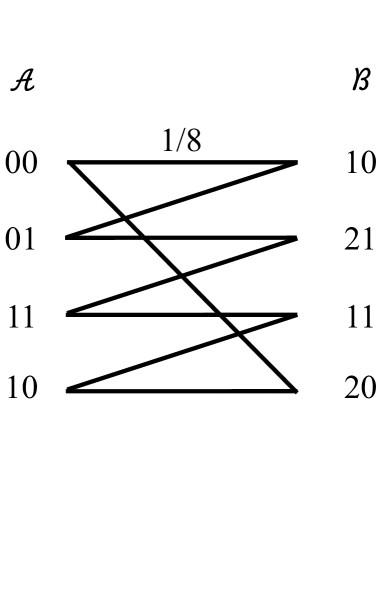
(a)

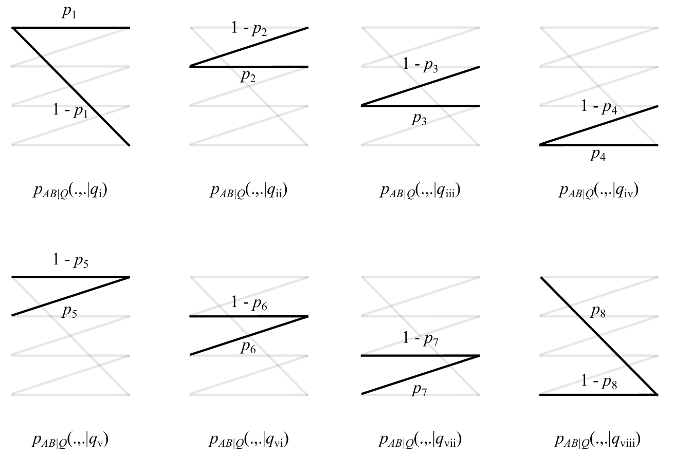
(b)

Figure 8: (a) Joint p.m.f. of $A,B$. Each solid line represents a probablity mass of 1/8. (b) Eight possible classes that $p_{AB|Q}(.,.|q)$ may belong to for a $p_{Q|AB}$ which satisfies $I(A;B|Q)=0$.

We will first show that there is no loss of generality in assuming that no more than one of the $q_{i}$’s is such that its $p_{AB|Q}(.,.|q_{i})$ belongs to the same class (and hence we may take $N=8$). Suppose, $q_{1}$ and $q_{2}$ belong to the same class, say class 1, with parameters $p_{1}$ and $p_{2}$ respectively. Then, if we denote the binary entropy function by $H_{2}(.)$, we have

$$H(A|QB)+H(B|QA)$$

$$=\sum_{k=1}^{N}p_{Q}(q_{k})\left(H(A|BQ=q_{k})+H(B|AQ=q_{k})\right)$$

$$=p_{Q}(q_{1})H_{2}(p_{1})+p_{Q}(q_{2})H_{2}(p_{2})$$

$$\qquad+\sum_{k=3}^{N}p_{Q}(q_{k})\left(H(A|BQ=q_{k})+H(B|AQ=q_{k})\right)$$

$$\leq\left(p_{Q}(q_{1})+p_{Q}(q_{2})\right)H_{2}\left(\frac{p_{Q}(q_{1})p_{1}+p_{Q}(q_{2})p_{2}}{p_{Q}(q_{1})+p_{Q}(q_{2})}\right)$$

$$\qquad+\sum_{k=3}^{N}p_{Q}(q_{k})\left(H(A|BQ=q_{k})+H(B|AQ=q_{k})\right),$$

where the inequality (Jensen’s) follows from the concavity of the binary entropy function. Thus, we can define a $Q^{\prime}$ of alphabet size $N-1$ where letters $q_{1},q_{2}$ are replaced by $q_{0}$ such that $p_{Q^{\prime}}(q_{0})=p_{Q}(q_{1})+p_{Q}(q_{2})$, and $p_{AB|Q^{\prime}=q_{0}}$ is in class 1 with parameter $\frac{p_{Q}(q_{1})p_{1}+p_{Q}(q_{2})p_{2}}{p_{Q}(q_{1})+p_{Q}(q_{2})}$, while maintaining for $i=3,\ldots,N$, $p_{Q^{\prime}}(q_{i})=p_{Q}(q_{i})$ and $p_{AB|Q^{\prime}}(a,b|q_{i})=p_{AB|Q}(a,b|q_{i})$. (It is easy to verify (a) that this gives a valid joint p.m.f. for $p_{ABQ^{\prime}}$, (b) that the induced $p_{AB}$ is the same as the original, and (c) that the induced $p_{Q^{\prime}|AB}$ satisfies the condition $I(A;B|Q^{\prime})=0$.) Then, the above inequality states that

$$H(A|QB)+H(B|QA)\leq H(AQ^{\prime}B)+H(B|Q^{\prime}A)$$

proving our claim.

Thus, without loss of generality, we may assume that $N=8$ and $p_{AB|Q}(\cdot,\cdot|q_{i})$ belongs to class $i$. Notice that

$$p_{Q|AB}(q_{1}|00,10)+p_{Q|AB}(q_{5}|00,10) =1,$$

$$p_{Q|AB}(q_{2}|01,10)+p_{Q|AB}(q_{5}|01,10) =1,$$

$$p_{Q|AB}(q_{2}|01,21)+p_{Q|AB}(q_{6}|01,21) =1,$$

$$p_{Q|AB}(q_{3}|11,21)+p_{Q|AB}(q_{6}|11,21) =1,$$

$$p_{Q|AB}(q_{3},11,11)+p_{Q|AB}(q_{7}|11,11) =1,$$

$$p_{Q|AB}(q_{4}|10,11)+p_{Q|AB}(q_{7}|10,11) =1,$$

$$p_{Q|AB}(q_{4}|10,20)+p_{Q|AB}(q_{8}|10,20) =1,$$

$$p_{Q|AB}(q_{1}|00,20)+p_{Q|AB}(q_{8}|00,20) =1.$$

Let us define

$$\tilde{p}_{1} \triangleq p_{Q|AB}(q_{1}|00,10), \tilde{p}_{5}\triangleq p_{Q|AB}(q_{5}|01,10),$$

$$\tilde{p}_{2} \triangleq p_{Q|AB}(q_{2}|01,21), \tilde{p}_{6}\triangleq p_{Q|AB}(q_{6}|11,21),$$

$$\tilde{p}_{3} \triangleq p_{Q|AB}(q_{3}|11,11), \tilde{p}_{7}\triangleq p_{Q|AB}(q_{7}|10,11),$$

$$\tilde{p}_{4} \triangleq p_{Q|AB}(q_{4}|10,20), \tilde{p}_{8}\triangleq p_{Q|AB}(q_{8}|00,20).$$

Let us evaluate $H(B|QA)$ in terms of the above parameters. Notice that $H(B|Q=q_{i},A)=0$ for $i=5,\ldots,8$. Hence

$$H(B|QA)$$

$$=\sum_{\begin{subarray}{c}(q,a)\in\{(1,00),(2,01),\\ \qquad\;\;\;\,(3,11),(4,10)\}\end{subarray}}p_{QA}(q,a)H(B|Q=q,A=a)$$

$$=\frac{\tilde{p}_{1}+(1-\tilde{p}_{8})}{8}H_{2}\left(\frac{\tilde{p}_{1}}{\tilde{p}_{1}+(1-\tilde{p}_{8})}\right)$$

$$\qquad+\frac{\tilde{p}_{2}+(1-\tilde{p}_{5})}{8}H_{2}\left(\frac{\tilde{p}_{2}}{\tilde{p}_{2}+(1-\tilde{p}_{5})}\right)$$

$$\qquad+\frac{\tilde{p}_{3}+(1-\tilde{p}_{6})}{8}H_{2}\left(\frac{\tilde{p}_{3}}{\tilde{p}_{3}+(1-\tilde{p}_{6})}\right)$$

$$\qquad+\frac{\tilde{p}_{4}+(1-\tilde{p}_{7})}{8}H_{2}\left(\frac{\tilde{p}_{4}}{\tilde{p}_{4}+(1-\tilde{p}_{7})}\right)$$

$$\leq\frac{4+\sum_{i=1}^{4}\tilde{p}_{i}-\sum_{j=5}^{8}\tilde{p}_{j}}{8},$$

where the inequality follows from the fact that binary entropy function is upperbounded by 1. Similary, we can get

$$H(A|QB)\leq\frac{4+\sum_{j=5}^{8}\tilde{p}_{j}-\sum_{i=1}^{4}\tilde{p}_{i}}{8}.$$

Combining, we obtain, as desired,

$$H(B|QA)+H(A|QB)\leq 1.$$

Remark

Note that we have actually shown that for bit-OT $(A,B)$, the intersection of $\mathfrak{T}({A};{B})$ on the plane $z=0$ is the increasing hull of the line segment between $(1,0,0)$ and $(0,1,0)$. This follows from what we showed above (i.e., $\inf\{R_{1}+R_{2}:(R_{1},R_{2},0)\in\mathfrak{T}({A};{B})\}=1$) combined with the fact that $T^{\mathrm{int}}_{1}({A};{B})=(1,0,0)$ and $T^{\mathrm{int}}_{2}({A};{B})=(0,1,0)$, and that $\mathfrak{T}({A};{B})$ is convex.

VI Conclusion

In this work, we introduced a multi-dimensional measure of correlation between two random variables, called the region of tension. We show that the region of tension yields an exact characterization of the rate-region of a 3-party communication problem, that extends the 2-party problem considered by Gács and Körner [9].

Further, relying on a monotonicity property of the region of tension in secure protocols, we show that the region of tension can be used to derive lowerbounds on the rate of securely sampling a pair of correlated random variables, using samples from another joint distribution as a setup. While we use this to obtain tight bounds for secure sampling in many problems, we leave open the question of whether there are cases where the bounds derived from the region of tension are loose. Another open problem is to derive tight lowerbounds for secure computation. We note that while bounds for secure sampling do yield bounds for secure computation, they tend to be loose, in general.

As defined here, the region of tension is for two correlated random variables. We leave it open to devise analogous notions for more than two parties, with analogous applications. (One such notion, applicable to a specialized context, was defined in [23].) Other potential directions of study include extending the region of tension to the setting of quantum information, and the possibility of basing the definition of tension on quantities other than mutual information.

Appendix A Details Omitted from Section II

Lemma A.1 (See Problem 3.4.25 in page 402 of [6])

Given a pair of random variables $(X,Y)$ and a p.m.f. ${p_{Q|XY}}$ such that $I(Y;Q|X)=I(X;Q|Y)=0$, there exists a p.m.f. $p_{Q^{\prime}|XY}$ such that $H(Q^{\prime}|X)=H(Q^{\prime}|Y)=0$ and $Q-Q^{\prime}-XY$.

Proof:

Suppose ${p_{Q|XY}}$ is such that $I(Y;Q|X)=I(X;Q|Y)=0$. Then

$$p_{Q|XY}(q|x,y) =p_{Q|X}(q|x)=p_{Q|Y}(q|y).$$

Hence, for all $(x,y)$ such that $p_{XY}(x,y)>0$, we must have $\forall q$, $p_{Q|X}(q|x)=p_{Q|Y}(q|y)$. This implies that, in the characteristic bipartite graph (which has vertices in $\mathcal{X}\cup\mathcal{Y}$ and an edge between $x\in\mathcal{X}$ and $y\in\mathcal{Y}$ if and only if $p_{XY}(x,y)>0$), for each connected component $C\subseteq\mathcal{X}\cup\mathcal{Y}$, there is a distribution $p^{C}_{Q}$ such that for all $x\in C\cap\mathcal{X}$ and all $q$, $p_{Q|X}(q|x)=p^{C}_{Q}(q)$; similarly, for all $y\in C\cap\mathcal{Y}$ and all $q$, $p_{Q|Y}(q|y)=p^{C}_{Q}(q)$. Define $p_{Q^{\prime}|XY}$ over the set of connected components in this graph such that, with probability 1, $Q^{\prime}$ is the connected component $C(X,Y)$ in this graph to which the vertices $X$ and $Y$ belong (and hence $H(Q^{\prime}|X)=H(Q^{\prime}|Y)=0$), and $p_{Q|Q^{\prime}}(q|C)=p^{C}_{Q}(q)$. Then $p_{Q|XY}(q|x,y)=p_{Q|X}(q|x)=p^{C(x,y)}_{Q}(q)=p_{Q|Q^{\prime}}(q|C(x,y))$, so that $Q-Q^{\prime}-XY$. ∎

The following calculation is useful in applying the above lemma in a couple of our proofs.

Lemma A.2

For correlated random variables $(X,Y,Q,Q^{\prime})$ if $H(Q^{\prime}|X)=0$ (or $H(Q^{\prime}|Y)=0$) and $Q-Q^{\prime}-XY$, then $I(X;Y|Q)\geq I(X;Y|Q^{\prime})$.

Proof:

$$I(X;Y|Q) \stackrel{{\scriptstyle\text{(a)}}}{{=}}I(X,Q^{\prime};Y|Q)$$

$$\geq I(X;Y|Q^{\prime},Q)$$

$$\stackrel{{\scriptstyle\text{(b)}}}{{=}}I(X;Y|Q^{\prime}),$$

where the (a) follows from $H(Q^{\prime}|X)=0$ and (b) from the Markov chain $Q-Q^{\prime}-XY$. ∎

Proof:

To prove (5), firstly note that $T^{\mathrm{int}}_{1}({X};{Y})=$

$$\inf_{\begin{subarray}{c}{p_{Q|XY}}:\\ I(X;Q|Y)=0\\ I(X;Y|Q)=0\end{subarray}}I(Y;Q|X)\leq\inf_{\begin{subarray}{c}{p_{Q|XY}}:\\ H(Q|Y)=0\\ I(X;Y|Q)=0\end{subarray}}H(Q|X),$$

because if $H(Q|Y)=0$ then $I(X;Q|Y)=0$ and $I(Y;Q|X)=H(Q|X)$. For the other direction, we invoke Lemma A.1 (with $X$ and $Q$ interchanged), so that given $Q$ such that $I(X;Q|Y)=I(X;Y|Q)=0$, $\exists Q^{\prime}$ such that $H(Q^{\prime}|Y)=H(Q^{\prime}|Q)=0$ and $X-Q^{\prime}-QY$; then $H(Q^{\prime}|X)=I(Y;Q^{\prime}|X)\leq I(Y;Q|X)$, and $X-Q^{\prime}-Y$. So $Q^{\prime}$ is considered in the $\inf$ expression of the RHS, and we have LHS $\geq$ RHS. This proves (5). Similarly, (6) holds.

To prove (7), firstly we note that $T^{\mathrm{int}}_{3}({X};{Y})=$

$$\inf_{\begin{subarray}{c}{p_{Q|XY}}:\\ I(Y;Q|X)=0\\ I(X;Q|Y)=0\end{subarray}}I(X;Y|Q)\leq\inf_{\begin{subarray}{c}{p_{Q|XY}}:\\ H(Q|X)=0\\ H(Q|Y)=0\end{subarray}}I(X;Y|Q),$$

since $H(Q|X)=H(Q|Y)=0$ implies that $I(Y;Q|X)=I(X;Q|Y)=0$. For the inequality in the other direction, by Lemma A.1, given $Q$ such that $I(Y;Q|X)=I(X;Q|Y)=0$, we get $Q^{\prime}$ such that $H(Q^{\prime}|X)=H(Q^{\prime}|Y)=0$ and $Q-Q^{\prime}-XY$; then, by Lemma A.2 it follows that $I(X;Y|Q)\geq I(X;Y|Q^{\prime})$. Hence, $\inf_{{p_{Q|XY}}:I(Y;Q|X)=I(X;Q|Y)=0}I(X;Y|Q)\geq\inf_{{p_{Q|XY}}:H(Q|X)=H(Q|Y)=0}I(X;Y|Q)$. Thus, (7) holds. ∎

Proof:

Consider any two points $s_{1},s_{2}\in\mathfrak{T}({X};{Y})$. Consider any point $s=\alpha s_{1}+(1-\alpha)s_{2}$ for $0\leq\alpha\leq 1$. We need to show that $s\in\mathfrak{T}({X};{Y})$ as well.

Since $s_{1},s_{2}\in\mathfrak{T}({X};{Y})$, there are random variables $p_{Q_{1}|XY}$ and $p_{Q_{2}|XY}$ such that $s_{1}^{\prime}:=T({X};{Y}|{Q_{1}})\leq s_{1}$ and $s_{2}^{\prime}:=T({X};{Y}|{Q_{2}})\leq s_{2}$. Let $J$ be a binary random variable independent of $(X,Y,Q_{1},Q_{2})$ taking on value 1 with probability $\alpha$ and 2 with probability $1-\alpha$. Let $Q=(J,Q_{J})$. Then $T({X};{Y}|{Q})=\alpha T({X};{Y}|{Q_{1}})+(1-\alpha)T({X};{Y}|{Q_{2}})$. That is, $s^{\prime}=\alpha s^{\prime}_{1}+(1-\alpha)s^{\prime}_{2}$ is in $\mathfrak{T}({X};{Y})$. Hence $s\in\mathfrak{T}({X};{Y})$, since $s\geq s^{\prime}$. ∎

Lemma A.3

If $A\subseteq\mathbb{R}^{m}$ is compact, then its increasing hull,

$$i\left(A\right)=\{x\in\mathbb{R}^{m}:x\geq a\text{ for some }a\in A\},$$

is closed.

Proof:

Let $\{x_{n}\}$ be a sequence in $i\left(A\right)$ converging to $x$. Then, there is a sequence $\{a_{n}\}$ in $A$ such that $x_{n}\geq a_{n}$, for all $n$. Since $A$ is compact, there is a convergent subsequence $\{a_{n_{k}}\}$ of $\{a_{n}\}$ that converges to $a\in A$. Also, the subsequence $\{x_{n_{k}}\}$ converges to $x$, and satisfies $x_{n_{k}}\geq a_{n_{k}}$, for all $k$. Thus, $x\geq\lim_{k\rightarrow\infty}a_{n_{k}}=a$, and so, $x\in i\left(A\right)$. ∎

The following simple (and standard) observation is used in proving Lemma II.6.

Lemma A.4

If $p_{Z}$ and $p_{Z^{\prime}}$ are such that $\Delta(Z,Z^{\prime})=\epsilon$, then there is a joint distribution $p_{JWW^{\prime}}$ such that $p_{W}=p_{Z}$, $p_{W^{\prime}}=p_{Z^{\prime}}$, $p_{J}(0)=\epsilon$ and $p_{J}(1)=1-\epsilon$ and $J=1\implies W=W^{\prime}$.

Proof:

First we define independent random variables $J$, $W_{0}$, $W_{1}$ and $W_{2}$ (the first one over $\{0,1\}$ and the others over the common alphabet of $Z$ and $Z^{\prime}$ as follows.

$$p_{J}(0) =\epsilon,\text{ and }p_{J}(1)=1-\epsilon,$$

$$p_{W_{0}}(z) =\frac{\min\{p_{Z}(z),p_{Z^{\prime}}(z)\}}{1-\epsilon},$$

$$p_{W_{1}}(z) =\frac{p_{Z}(z)-(1-\epsilon)\cdot p_{W_{0}}(z)}{\epsilon},$$

$$p_{W_{2}}(z) =\frac{p_{Z^{\prime}}(z)-(1-\epsilon)\cdot p_{W_{0}}(z)}{\epsilon}.$$

We define $W$ and $W^{\prime}$ in terms of these random variables: when $J=1$, $W=W^{\prime}=W_{0}$, and when $J=0$ we set $W=W_{1}$ and $W^{\prime}=W_{2}$. It is easy to verify that the resulting random variables have the correct marginals. ∎

Lemma II.6

Suppose random variables $(A,B,C)$ and $(A^{\prime},B^{\prime},C^{\prime})$ over the same alphabet $\mathcal{A}\times\mathcal{B}\times\mathcal{C}$ are such that $\Delta(ABC,A^{\prime}B^{\prime}C^{\prime})=\epsilon$. Then $I(A^{\prime};B^{\prime}|C^{\prime})\leq I(A;B|C)+2H_{2}(\epsilon)+\epsilon\log\min\{|\mathcal{A}|,|\mathcal{B}|\}$.

Proof:

We apply Lemma A.4 with $Z=(A,B,C)$ and $Z^{\prime}=(A^{\prime},B^{\prime},C^{\prime})$ to obtain a joint distribution $p_{J,A,B,C,A^{\prime},B^{\prime},C^{\prime}}$ so that $J=1\implies(A,B,C)=(A^{\prime},B^{\prime},C^{\prime})$ and this event occurs with probability $1-\epsilon$.

Now, note that

$$I(A;B|C) =I(A;BJ|C)-I(A;J|BC)$$

$$=I(A;B|CJ)+I(A;J|C)-I(A;J|BC).$$

Since $0\leq I(A;J|C)\leq H(J)$ and $0\leq I(A;J|BC)\leq H(J)$, we have

$$|I(A;B|C)-I(A;B|CJ)|\leq H(J)=H_{2}(\epsilon)$$ (52)

The same condition holds for $A^{\prime},B^{\prime},C^{\prime}$ instead of $A,B,C$. Hence

$$I(A^{\prime};B^{\prime}|C^{\prime})\leq I(A^{\prime};B^{\prime}|C^{\prime}J)+H_{2}(\epsilon)$$

$$\qquad=(1-\epsilon)I(A^{\prime};B^{\prime}|C^{\prime},J=1)$$

$$\qquad\qquad\qquad\qquad+\epsilon I(A^{\prime};B^{\prime}|C^{\prime},J=0)+H_{2}(\epsilon)$$

$$\qquad=(1-\epsilon)I(A;B|C,J=1)$$

$$\qquad\qquad\qquad\qquad+\epsilon I(A^{\prime};B^{\prime}|C^{\prime},J=0)+H_{2}(\epsilon)$$

$$\qquad=I(A;B|CJ)-\epsilon I(A;B|C,J=0)$$

$$\qquad\qquad\qquad\qquad+\epsilon I(A^{\prime};B^{\prime}|C^{\prime},J=0)+H_{2}(\epsilon)$$

$$\qquad\stackrel{{\scriptstyle\mathrm{(a)}}}{{\leq}}I(A;B|C)+\epsilon I(A^{\prime};B^{\prime}|C^{\prime},J=0)+2H_{2}(\epsilon)$$

$$\qquad\leq I(A;B|C)+\epsilon\min\{\log|\mathcal{A}|,\log|\mathcal{B}|\}+2H_{2}(\epsilon),$$

where (a) follows from (52). ∎

Appendix B Details Omitted from Section III

Proof:

The first equation (12) follows immediately from Theorem III.1. We need to show (13) which is repeated below for convenience.

$$\mathfrak{T}({X};{Y}) =i\left(f_{X,Y}({\mathcal{R}}_{\text{\sf ACI}}(X;Y))\right) \qquad\eqref{eq:Rtens-ACI}$$

where $f_{X,Y}$ is an affine map defined as

$$f_{X,Y}\left(\left[\begin{array}[]{c}R_{1}\\ R_{2}\\ R_{\text{\sf CI}}\end{array}\right]\right)\triangleq\left[\begin{array}[]{c}R_{1}\\ R_{2}\\ I(X;Y)+R_{1}+R_{2}-R_{\text{\sf CI}}\end{array}\right].$$

Given a $p_{Q|XY}$ and $(r_{1},r_{2},r_{\text{\sf CI}})$ such that $r_{1}\geq I(Y;Q|X)$, $r_{2}\geq I(X;Q|Y)$ and $r_{\text{\sf CI}}\leq I(XY;Q)$, we have

$$r_{1} +r_{2}-r_{\text{\sf CI}}+I(X;Y)$$

$$\geq I(Y;Q|X)+I(X;Q|Y)-I(XY;Q)+I(X;Y)$$

$$=I(X;Y|Q),$$

where the last equality is (51). Thus, $\mathrm{L.H.S.}\supseteq\mathrm{R.H.S.}$

If $(r^{\prime}_{1},r^{\prime}_{2},r^{\prime}_{3})\in\mathfrak{T}({X};{Y})$, then there is a $p_{Q|XY}$ such that $r^{\prime}_{1}\geq I(Y;Q|X)$, $r^{\prime}_{2}\geq I(X;Q|Y)$ and $r^{\prime}_{3}\geq I(X;Y|Q)$. But, since (51) implies that $(I(Y;Q|X),I(X;Q|Y),I(X;Y|Q))\in f_{X,Y}({\mathcal{R}}_{\text{\sf ACI}}(X;Y))$, we have $(r^{\prime}_{1},r^{\prime}_{2},r^{\prime}_{3})\in i\left(f_{X,Y}({\mathcal{R}}_{\text{\sf ACI}}(X;Y))\right)$. Thus, $\mathrm{L.H.S.}\subseteq\mathrm{R.H.S.}$

∎

Proof:

From the definitions it is clear that, ${\mathrm{C}}_{\text{\sf$\text{\sf GK}$}}(X;Y)\leq{{\mathcal{R}}_{\text{\sf ACI}}}_{,3}^{\mathrm{int}}({X};{Y})$. But as we will show, this is in fact an equality. Theorem III.1 implies that

$${{\mathcal{R}}_{\text{\sf ACI}}}_{,3}^{\mathrm{int}}({X};{Y}) =\max_{\begin{subarray}{c}p_{Q|XY}:\\ I(X;Q|Y)=I(Y;Q|X)=0\end{subarray}}I(XY;Q).$$ (53)

By Lemma A.1, given ${p_{Q|XY}}$ such that $I(X;Q|Y)=I(Y;Q|X)=0$, we can find a random variable $Q^{\prime}$ with $H(Q^{\prime}|X)=H(Q^{\prime}|Y)=0$ and $Q-Q^{\prime}-(X,Y)$ is a Markov chain. Then, clearly, $I(X;Q^{\prime}|Y)=I(Y;Q^{\prime}|X)=0$ and furthermore

$$I(XY;Q)\leq I(XY;QQ^{\prime})=I(XY;Q^{\prime})=H(Q^{\prime}).$$

Hence,

$${{\mathcal{R}}_{\text{\sf ACI}}}_{,3}^{\mathrm{int}}({X};{Y}) =\max_{p_{Q^{\prime}|XY}:H(Q^{\prime}|X)=H(Q^{\prime}|Y)=0}H(Q^{\prime}).$$

Since $H(Q^{\prime}|X)=H(Q^{\prime}|Y)=0$, $Q^{\prime}=f_{1}(X)$ and $Q^{\prime}=f_{2}(Y)$ for some functions $f_{1}$ and $f_{2}$, and hence ${\mathrm{C}}_{\text{\sf$\text{\sf GK}$}}(X;Y)\geq H(Q^{\prime})$. So, ${\mathrm{C}}_{\text{\sf$\text{\sf GK}$}}(X;Y)\geq{{\mathcal{R}}_{\text{\sf ACI}}}_{,3}^{\mathrm{int}}({X};{Y})$. Hence, we can conclude (14)-(15).

It only remains to show

$$T^{\mathrm{int}}_{3}({X};{Y})=I(X;Y)-{{\mathcal{R}}_{\text{\sf ACI}}}_{,3}^{\mathrm{int}}({X};{Y}).$$ (54)

This easily follows from (4) and (53) using (48)-(50). ∎

Proof:

We are given $p^{\vphantom{\ast}}_{X,Y}$, $p^{\ast}_{Q|XY}$, $d$. Also, we have

$$D^{\ast}={\mathbb{E}}_{p^{\vphantom{\ast}}_{X,Y}p^{\ast}_{Q|XY}}\left[d(X,Y,Q)\right].$$

This proof uses the notion of typicality. We will use notation, definitions, and results from [8]. All typical sequences are defined with respect to the joint distribution $p^{\vphantom{\ast}}_{X,Y}p^{\ast}_{Q|XY}$. For a positive integer $k$, we will denote $\{1,\ldots,k\}$ by $[k]$.

Random codebook construction: Let $\epsilon^{\prime}>0$ and $p_{Q}(q)=\sum_{x,y}p^{\vphantom{\ast}}_{X,Y}(x,y)p^{\ast}_{Q|XY}(q|x,y)$ be the marginal distribution of $Q$ induced by the given joint distribution. Let $r,r_{1},r_{2}$ be such that $r\geq r_{1},r_{2}$. We generate $2^{nr}$ codewords $Q^{n}(l),l\in[2^{nr}]$ randomly and independently each according to $\prod_{i=1}^{n}p_{Q}(q_{i})$. The set of indices $l\in[2^{nr}]$ is then partitioned in two different ways into equal size subsets: 1-bins $\mathcal{B}_{1}(m_{1})=\{(m_{1}-1)2^{n(r-r_{1})}+1,\ldots,m_{1}2^{n(r-r_{1})}\},m_{1}\in[2^{nr_{1}}]$, and 2-bins $\mathcal{B}_{2}(m_{2})=\{(m_{2}-1)2^{n(r-r_{2})}+1,\ldots,m_{2}2^{n(r-r_{2})}\},m_{2}\in[2^{nr_{2}}]$.

Encoding: If the input to the encoder is $(x^{n},y^{n})$, it finds an index $l$ such that $(x^{n},y^{n},q^{n}(l))\in{\mathcal{T}}^{(n)}_{\epsilon^{\prime}}(X,Y,Q)$. If none is available, $l$ is chosen uniformly at random from $[2^{nr}]$. The encoder sends to the $k$-th receiver, $k=1,2$, the bin index $m_{k}$ such that $l\in\mathcal{B}_{k}(m_{k})$, i.e., $f^{(n)}_{k}(x^{n},y^{n})=m_{k}$, $k=1,2$.

Decoding: The first decoder, on receiving $m_{1}$, tries to find a unique $\hat{l}_{1}\in\mathcal{B}_{1}(m_{1})$ such that $(x^{n},q^{n}(\hat{l}_{1}))\in{\mathcal{T}}^{(n)}_{\epsilon^{\prime}}(X,Q)$. If it cannot find such an $\hat{l}_{1}$, it sets $\hat{l}_{1}=1$. Decoder 1 outputs $\hat{l}_{1}$, i.e., $g^{(n)}_{1}(x^{n},m_{1})=\hat{l}_{1}$. Similarly, decoder 2 outputs a $\hat{l}_{2}$ it finds using $y^{n},m_{2}$, and $\mathcal{B}_{2}$.

Reconstruction: The reconstruction function $h^{(n)}$ is defined as $h^{(n)}(l)=q^{n}(l)$. Thus the output sequence is

$$q^{n}=h^{(n)}(\hat{l}_{1})=q^{n}(\hat{l}_{1}).$$

Analysis of the probability of error and expected distortion: Let $L,M_{1},M_{2},\widehat{L}_{1},\widehat{L}_{2}$ be the indices chosen by the encoder and the decoder. We define the error event as

$\supseteq$: Let $s=(H(X)-R_{\text{\sf C}},H(Y)-R_{\text{\sf C}},R_{\text{\sf C}})\in{\mathcal{R}}_{\text{\sf GW}}$. Then (a) $R_{C}\leq I(X;Y)$ since $s\in\mathcal{L}_{\text{\sf GW}}$, and (b) if $s^{\prime}=(r_{\text{\sf A}},r_{\text{\sf B}},R_{\text{\sf C}})\in\mathcal{L}_{\text{\sf GW}}$, then since $r_{\text{\sf A}}\geq H(X)-R_{\text{\sf C}}$ and $r_{\text{\sf B}}\geq H(Y)-R_{\text{\sf C}}$, we have $s^{\prime}\geq s$ (component-wise) which implies that $s^{\prime}\in{\mathcal{R}}_{\text{\sf GW}}$ from the definition of the GW system. ∎

Proof:

$${\mathrm{C}}_{\text{\sf$\sf Wyner$}} =\inf\{R_{\text{\sf C}}:(R_{\text{\sf A}},R_{\text{\sf B}},R_{\text{\sf C}})\in{\mathcal{R}}_{\text{\sf GW}},$$

$$\qquad\qquad\qquad R_{\text{\sf A}}+R_{\text{\sf B}}+R_{\text{\sf C}}=H(X,Y)\}$$

$$\stackrel{{\scriptstyle\mathrm{(a)}}}{{=}}\inf\{R_{1}+R_{2}+I(X;Y):(R_{1},R_{2},0)\in{\mathcal{R}}_{\text{\sf GW}}^{\prime}\}$$

$$\stackrel{{\scriptstyle\mathrm{(b)}}}{{=}}\inf\{R_{1}+R_{2}+I(X;Y):(R_{1},R_{2},0)\in\mathfrak{T}({X};{Y})\},$$

where (a) follows from the definition ${\mathcal{R}}_{\text{\sf GW}}^{\prime}=f({\mathcal{R}}_{\text{\sf GW}})$; (b) follows from Theorem IV.3: $\geq$ direction follows directly from the theorem. But $>$ cannot hold, since by the theorem, if $(R_{1},R_{2},0)\in\mathfrak{T}({X};{Y})$ then there exists $(R_{1}^{\prime},R_{2}^{\prime},0)\in{\mathcal{R}}_{\text{\sf GW}}^{\prime}$ such that $R_{1}^{\prime}\leq R_{1}$ and $R_{2}^{\prime}\leq R_{2}$.

∎

Proof:

$$G(Y\rightarrow X)$$

$$\quad=\inf\{R_{\text{\sf C}}:(H(X|Y),H(Y)-R_{\text{\sf C}},R_{\text{\sf C}})\in{\mathcal{R}}_{\text{\sf GW}}\},$$

$$\quad\stackrel{{\scriptstyle\mathrm{(a)}}}{{=}}\inf\{R:(R-I(X;Y),0,0)\in{\mathcal{R}}_{\text{\sf GW}}^{\prime}\}$$

$$\quad\stackrel{{\scriptstyle\mathrm{(b)}}}{{=}}\inf\{R:(R-I(X;Y),0,0)\in\mathfrak{T}({X};{Y})\}$$

$$\quad\stackrel{{\scriptstyle\mathrm{(c)}}}{{=}}I(X;Y)+T^{\mathrm{int}}_{1}({X};{Y}),$$

where (a) follows from ${\mathcal{R}}_{\text{\sf GW}}^{\prime}=f({\mathcal{R}}_{\text{\sf GW}})$. (b) is a consequence of Theorem IV.3: And (c) follows from the definition of $T^{\mathrm{int}}_{1}({X};{Y})$.

Similarly we get (37). The equality (38) is proved in [17] which along with (36)-(37) implies (39).

∎

Appendix D Details Omitted from Section V

Here we prove Theorem V.6. The following lemma will be useful in this.

Lemma D.1

Suppose ${\Pi}^{(X,Y)}\overset{\epsilon}{\leadsto}{(U,V)}$. Then

$$I(\Pi^{\mathrm{view}}_{\mathrm{Alice}};\Pi^{\mathrm{out}}_{\mathrm{Bob}}|\Pi^{\mathrm{out}}_{\mathrm{Alice}}) \leq 2\delta(\epsilon)$$

$$I(\Pi^{\mathrm{view}}_{\mathrm{Bob}};\Pi^{\mathrm{out}}_{\mathrm{Alice}}|\Pi^{\mathrm{out}}_{\mathrm{Bob}}) \leq 2\delta(\epsilon)$$

where $\delta(\epsilon)=2H_{2}(\epsilon)+\epsilon\log\max\{|\mathcal{U}|,|\mathcal{V}|\}$.

Proof:

We show $I(\Pi^{\mathrm{view}}_{\mathrm{Alice}};\Pi^{\mathrm{out}}_{\mathrm{Bob}}|\Pi^{\mathrm{out}}_{\mathrm{Alice}})\leq 2\delta(\epsilon)$ (the other relation following similarly). Let $\Sigma^{\mathrm{view}}_{\mathrm{Alice}}$ be as in Definition V.4. Then $I(\Sigma^{\mathrm{view}}_{\mathrm{Alice}};V|U)=0$ and $\Delta(\Sigma^{\mathrm{view}}_{\mathrm{Alice}}V,\Pi^{\mathrm{view}}_{\mathrm{Alice}}\Pi^{\mathrm{out}}_{\mathrm{Bob}})\leq\epsilon$. Also, we have $\Delta(UV,\Pi^{\mathrm{out}}_{\mathrm{Alice}}\Pi^{\mathrm{out}}_{\mathrm{Bob}})\leq\epsilon$. Then

$$I(\Pi^{\mathrm{view}}_{\mathrm{Alice}};\Pi^{\mathrm{out}}_{\mathrm{Bob}}|\Pi^{\mathrm{out}}_{\mathrm{Alice}})$$

$$\qquad=I(\Pi^{\mathrm{view}}_{\mathrm{Alice}};\Pi^{\mathrm{out}}_{\mathrm{Bob}}|\Pi^{\mathrm{out}}_{\mathrm{Alice}})-I(\Sigma^{\mathrm{view}}_{\mathrm{Alice}};V|U)$$

$$\qquad\stackrel{{\scriptstyle\mathrm{(a)}}}{{=}}\Big{[}H(\Pi^{\mathrm{out}}_{\mathrm{Bob}}|\Pi^{\mathrm{out}}_{\mathrm{Alice}})-H(V|U)\Big{]}$$

$$\qquad\qquad\qquad-H(\Pi^{\mathrm{out}}_{\mathrm{Bob}}|\Pi^{\mathrm{view}}_{\mathrm{Alice}})+H(V|U\Sigma^{\mathrm{view}}_{\mathrm{Alice}})$$

$$\qquad=\Big{[}H(\Pi^{\mathrm{out}}_{\mathrm{Bob}}|\Pi^{\mathrm{out}}_{\mathrm{Alice}})-H(V|U)\Big{]}$$

$$\qquad\qquad\qquad+\Big{[}H(V|\Sigma^{\mathrm{view}}_{\mathrm{Alice}})-H(\Pi^{\mathrm{out}}_{\mathrm{Bob}}|\Pi^{\mathrm{view}}_{\mathrm{Alice}})\Big{]}$$

$$\qquad\qquad\qquad-I(V;U|\Sigma^{\mathrm{view}}_{\mathrm{Alice}})$$

$$\qquad\stackrel{{\scriptstyle\mathrm{(b)}}}{{\leq}}2\delta(\epsilon)$$

where in (a) we used $H(\Pi^{\mathrm{out}}_{\mathrm{Bob}}|\Pi^{\mathrm{view}}_{\mathrm{Alice}}\Pi^{\mathrm{out}}_{\mathrm{Alice}})=H(\Pi^{\mathrm{out}}_{\mathrm{Bob}}|\Pi^{\mathrm{view}}_{\mathrm{Alice}})$ (because $\Pi^{\mathrm{out}}_{\mathrm{Alice}}$ is a function of $\Pi^{\mathrm{view}}_{\mathrm{Alice}}$) and in (b) we bounded the two terms in the square brackets by invoking Lemma II.6 twice, with $((ABC),(A^{\prime}B^{\prime}C^{\prime}))$ being $((VVU),(\Pi^{\mathrm{out}}_{\mathrm{Bob}}\Pi^{\mathrm{out}}_{\mathrm{Bob}}\Pi^{\mathrm{out}}_{\mathrm{Alice}}))$ and $((VV\Sigma^{\mathrm{view}}_{\mathrm{Alice}}),(\Pi^{\mathrm{out}}_{\mathrm{Bob}}\Pi^{\mathrm{out}}_{\mathrm{Bob}}\Pi^{\mathrm{view}}_{\mathrm{Alice}}))$ respectively. ∎

Proof:

Suppose there is a protocol $\Pi$ such that ${\Pi}^{(X^{n_{2}},Y^{n_{2}})}\overset{\epsilon}{\leadsto}{(U^{n_{1}},V^{n_{1}})}$, for $\frac{n_{1}}{n_{2}}\geq r-\epsilon^{\prime}$. We will denote the final views of the two parties in this protocol by $(\Pi^{\mathrm{view}}_{\mathrm{Alice}},\Pi^{\mathrm{view}}_{\mathrm{Bob}})$. Also, we shall denote the outputs by $(\Pi^{\mathrm{out}}_{\mathrm{Alice}},\Pi^{\mathrm{out}}_{\mathrm{Bob}})$. Then, firstly, by conditions (1) and (2) of Definition V.2,

$$\mathcal{M}({\Pi^{\mathrm{view}}_{\mathrm{Alice}}};{\Pi^{\mathrm{view}}_{\mathrm{Bob}}})\supseteq\mathcal{M}({X^{n_{2}}};{Y^{n_{2}}}).$$

Secondly, by Lemma D.1, for random variables $(\Pi^{\mathrm{view}}_{\mathrm{Alice}},\Pi^{\mathrm{out}}_{\mathrm{Alice}},\Pi^{\mathrm{out}}_{\mathrm{Bob}},\Pi^{\mathrm{view}}_{\mathrm{Bob}})$, the hypothesis in condition (3^′) of Definition V.6 holds, with $\phi=\widehat{\phi}(\epsilon)\cdot n_{1}\cdot\log|\mathcal{U}||\mathcal{V}|$ where we set $\widehat{\phi}(\epsilon)=2(2H_{2}(\epsilon)+\epsilon)$. Hence

$$\mathcal{M}({\Pi^{\mathrm{out}}_{\mathrm{Alice}}};{\Pi^{\mathrm{out}}_{\mathrm{Bob}}}) \supseteq\mathcal{M}({\Pi^{\mathrm{view}}_{\mathrm{Alice}}};{\Pi^{\mathrm{view}}_{\mathrm{Bob}}})$$

$$\qquad\qquad+c\widehat{\phi}(\epsilon)\cdot n_{1}\log|\mathcal{U}||\mathcal{V}|,$$

where $c$ is as in Definition V.6. Finally, since $\Delta(U^{n_{1}}V^{n_{1}},\Pi^{\mathrm{out}}_{\mathrm{Alice}}\Pi^{\mathrm{out}}_{\mathrm{Bob}})\leq\epsilon$, by the continuity of $\mathcal{M}$ (condition (3^′′) of Definition V.6), we have

$$\mathcal{M}({U^{n_{1}}};{V^{n_{1}}}) \supseteq\mathcal{M}({\Pi^{\mathrm{out}}_{\mathrm{Alice}}};{\Pi^{\mathrm{out}}_{\mathrm{Bob}}})$$

$$\qquad\qquad+\widehat{\delta}(\epsilon)\cdot n_{1}\log|\mathcal{U}||\mathcal{V}|,$$

where $\widehat{\delta}(\epsilon)$ is as in condition (3^′′) of Definition V.6. Putting these together, after dividing throughout by $n_{1}$ (using condition (4) in Definition V.2 and convexity from condition (3^′′)), and using $\frac{n_{2}}{n_{1}}\leq\frac{1}{r-\epsilon^{\prime}}$, we get

$$\mathcal{M}({U};{V})\supseteq\frac{1}{r-\epsilon^{\prime}}\mathcal{M}({X};{Y})+\widehat{\delta}^{\prime}(\epsilon)\cdot\log|\mathcal{U}||\mathcal{V}|,$$

where $\widehat{\delta}^{\prime}(\epsilon)=c\widehat{\phi}(\epsilon)+\widehat{\delta}(\epsilon)$.

If the rate of statistically securely sampling $(U,V)$ from $(X,Y)$ is $r$, then for all $\epsilon,\epsilon^{\prime}>0$, the above relation should hold. Since $\widehat{\delta}^{\prime}(\epsilon)\downarrow 0$ as $\epsilon\downarrow 0$ and the regions $\mathcal{M}({U};{V})$ and $\mathcal{M}({X};{Y})$ are closed (condition (3^′′)), we get

$$\mathcal{M}({U};{V})\supseteq\frac{1}{r}\mathcal{M}({X};{Y})$$

as required. ∎

References

- [1] R. Ahlswede and J. Körner, “On common information and related characteristics of correlated information sources,” in Proc. of the 7th Prague Conference on Information Theory, 1974.
- [2] D. Beaver, “Correlated pseudorandomness and the complexity of private computations,” in Proc. th STOC, pp. 479–488, ACM, 1996.
- [3] D. Beaver, “Precomputing oblivious transfer,” in Don Coppersmith, editor, CRYPTO, vol. 963 of Lecture Notes in Computer Science, pp. 97–109, Springer, 1995.
- [4] T. M. Cover and J. A. Thomas, Elements of Information Theory, 2ed, Wiley, 2006.
- [5] I. Csiszár and R. Ahlswede, “On oblivious transfer capacity,” in Proc. International Symposium on Information Theory (ISIT), pp. 2061–2064, 2007.
- [6] I. Csiszár and J. Körner, Information Theory: Coding Theorems for Discrete Memorless Systems, 1ed, Akadémiai Kiadó, Budapest, 1981.
- [7] Y. Dodis and S. Micali, “Lower bounds for oblivious transfer reductions,” in Jacques Stern, editor, EUROCRYPT, vol. 1592 of Lecture Notes in Computer Science, pp. 42–55, Springer, 1999.
- [8] A. El Gamal and Y.-H. Kim, Network Information Theory, Cambridge, 2012.
- [9] P. Gács and J. Körner, “Common information is far less than mutual information,” Problems of Control and Information Theory, vol. 2, no. 2, pp. 119–162, 1973.
- [10] M. Gastpar, B. Rimoldi, and M. Vetterli, “To code or not to code: Lossy source-channel communication revisited,” IEEE Transactions on Information Theory, vol. 49, no. 5, pp. 1147–1158, 2003.
- [11] R. M. Gray and A. D. Wyner, “Source coding for a simple network,” Bell System Technical Journal, vol. 53, no. 9, pp. 1681–1721, 1974.
- [12] H. Imai, K. Morozov, and A. C. A. Nascimento, “On the oblivious transfer capacity of the erasure channel,” in Proc. International Symposium on Information Theory (ISIT), pp. 1428–1431, 2006.
- [13] H. Imai, K. Morozov, and A. C. A. Nascimento, “Efficient oblivious transfer protocols achieving a non-zero rate from any non-trivial noisy correlation,” in Proc. International Conference on Information Theoretic Security (ICITS), 2007.
- [14] H. Imai, K. Morozov, A. C. A. Nascimento, and A. Winter, “Efficient protocols achieving the commitment capacity of noisy correlations,” in Proc. International Symposium on Information Theory (ISIT), pp. 1432–1436, 2006.
- [15] H. Imai, J. Müller-Quade, A. C. A. Nascimento, and A. Winter, “Rates for bit commitment and coin tossing from noisy correlation,” in Proc. International Symposium on Information Theory (ISIT), pp. 45, 2004.
- [16] Y. Ishai, E. Kushilevitz, R. Ostrovsky, and A. Sahai, “Extracting Correlations.” in Proc. th FOCS, pp. 261–270, IEEE, 2009.
- [17] S. Kamath and V. Anantharam, “A new dual to the Gács-Körner common information defined via the Gray-Wyner system,” in Proc. 48th Allerton Conf. on Communication, Control, and Computing, pp. 1340–1346, 2010.
- [18] J. Kilian, “Founding cryptography on oblivious transfer,” in Proc. th STOC, pp. 20–31, ACM, 1988.
- [19] J. Kilian, “More general completeness theorems for secure two-party computation,” in Proc. nd STOC, pp. 316–324, ACM, 2000.
- [20] D. Marco and M. Effros, “On lossless coding with coded side information,” IEEE Transactions on Information Theory, vol. 55, no. 7, pp. 3284–3296, 2009.
- [21] V. M. Prabhakaran and M. M. Prabhakaran, “Assisted common information,” in Proc. International Symposium on Information Theory (ISIT), pp. 2602-2606, 2010.
- [22] V. M. Prabhakaran and M. M. Prabhakaran, “Assisted common information: Further results,” in Proc. International Symposium on Information Theory (ISIT), pp. 2861 - 2865, 2011.
- [23] M. M. Prabhakaran and V. M. Prabhakaran, “On secure multiparty sampling for more than two parties,” in Proc. IEEE Information Theory Workshop (ITW), pp. 99 - 103, 2012.
- [24] M. Rabin. “How to exchange secrets by oblivious transfer,” Technical Report TR-81, Harvard Aiken Computation Laboratory, 1981.
- [25] Stephen Wiesner. “Conjugate coding,” Sigact News, vol. 15, pp. 78–88, 1983.
- [26] S. Winkler and J. Wullschleger. “On the Efficiency of Classical and Quantum Oblivious Transfer Reductions,” in Tal Rabin, editor, CRYPTO, vol. 6223 of Lecture Notes in Computer Science, pp. 707–723, Springer, 2010.
- [27] A. Winter, A. C. A. Nascimento, and H. Imai. “Commitment capacity of discrete memoryless channels,” in Kenneth G. Paterson, editor, IMA Int. Conf., vol. 2898 of Lecture Notes in Computer Science, pp. 35–51, Springer, 2003.
- [28] H. S. Witsenhausen, “On sequences of pairs of dependent random variables,” SIAM Journal of Applied Mathematics, 28:100–113, 1975.
- [29] S. Wolf and J. Wullschleger. “Oblivious Transfer Is Symmetric,” in Serge Vaudenay, editor, EUROCRYPT, vol. 4004 of Lecture Notes in Computer Science, pp. 222–232, Springer, 2006.
- [30] S. Wolf and J. Wullschleger. “New monotones and lower bounds in unconditional two-party computation,” IEEE Transactions on Information Theory, vol. 54, no. 6, pp. 2792–2797, 2008.
- [31] J. Wullschleger. Oblivious-Transfer Amplification. Ph.D. thesis, Swiss Federal Institute of Technology, Zürich, 2008. http://arxiv.org/abs/cs.CR/0608076.
- [32] A. D. Wyner, “The common information of two dependent random variables,” IEEE Transactions on Information Theory, vol. 21, no. 2, pp. 163–179, 1975.
- [33] A. D. Wyner and J. Ziv, “Rate-distortion function for source coding with side information at the decoder,” IEEE Transactions on Information Theory, vol. 22, no. 1, pp. 1–11, 1976.
- [34] H. Yamamoto, “Coding theorems for Shannon’s cipher system with correlated source outputs, and common information,” IEEE Transactions on Information Theory, vol. 40, no. 1, pp. 85–95, 1994.