Holographic Lifshitz flows and the null energy condition

Abstract

We study asymptotically Lifshitz spacetimes and the constraints on flows between Lifshitz fixed points imposed by the null energy condition. In contrast with the relativistic holographic $c$-theorem, where the effective AdS radius, $L$, is monotonically decreasing in the IR, for Lifshitz backgrounds we find that both $L$ and $z$ may flow in either direction. We demonstrate this with several numerical examples in a phenomenological model with a massive gauge field coupled to a real scalar.

I Introduction

It is well known that energy conditions in general relativity play a crucial role in understanding the global structure of spacetime. In particular, such conditions are used as inputs to the Penrose-Hawking singularity theorems as well as the Hawking area theorem of black hole thermodynamics. Of particular interest is the null energy condition, which states that

$$T_{\mu\nu}k^{\mu}k^{\nu}\geq 0,$$ (1)

for any null vector field $k^{\mu}$. While this is a requirement imposed on the matter content of the theory, application of the Einstein equation

$$R_{\mu\nu}-{\textstyle\frac{1}{2}}g_{\mu\nu}R=8\pi GT_{\mu\nu},$$ (2)

immediately converts this to a condition on the geometry

$$R_{\mu\nu}k^{\mu}k^{\nu}\geq 0.$$ (3)

As an example of how the null energy condition is applied, consider an affinely parametrized null congruence specified by $k^{\mu}\partial_{\mu}=d/d\lambda$. The Raychaudhuri equation then gives

$$\frac{d\theta}{d\lambda}=-\frac{1}{D-2}\theta^{2}-\sigma_{\mu\nu}\sigma^{\mu\nu}+\omega_{\mu\nu}\omega^{\mu\nu}-R_{\mu\nu}k^{\mu}k^{\nu},$$ (4)

where $\theta$ is the expansion of the null congruence, $\sigma_{\mu\nu}$ the shear and $\omega_{\mu\nu}$ the twist. (Here $D$ is the dimension of spacetime.) So long as the congruence is twist-free and the null energy condition is satisfied, the right hand side is then non-positive, and we may conclude that $d\theta/d\lambda\leq 0$. Moreover, in this case the inequality $d\theta/d\lambda\leq-\theta^{2}/(D-2)$ may be integrated to demonstrate that any negative expansion necessarily leads to the formation of caustics.

Turning to AdS/CFT, the null energy condition plays a key role in the proof of the holographic $c$-theorem concerning flows between the UV and IR Alvarez:1998wr ; Girardello:1998pd ; Freedman:1999gp ; Sahakian:1999bd . In particular, working in the Poincaré patch and assuming $d$-dimensional Lorentz invariance, the bulk metric may be parametrized as

$$ds_{d+1}^{2}=e^{2A}(-dt^{2}+d\vec{x}_{d-1}^{\,2})+dr^{2},$$ (5)

where $A$ is a function of the bulk radial coordinate $r$. For pure AdS, this function takes the form $A=r/L_{0}$, where $L_{0}$ is the AdS radius. However, more generally, we may define an effective AdS radius $L(r)$ along flows according to $A^{\prime}(r)=1/L(r)$, or equivalently $L(r)=1/A^{\prime}(r)$, where primes denote derivatives with respect to $r$. This effective radius agrees with the true AdS radius at fixed points of the flow.

The bulk metric (5) has the form of a domain wall solution, and the Ricci tensor is easily computed:

$$R_{\mu\nu}=-(A^{\prime\prime}+dA^{\prime 2})g_{\mu\nu},\qquad R_{rr}=-d(A^{\prime\prime}+A^{\prime 2}).$$ (6)

Choosing a null vector field $k^{\mu}\partial_{\mu}=e^{-A}\partial_{t}+\partial_{r}$, the null energy condition in the bulk then translates to the Ricci condition (3), which reads

$$e^{-2A}R_{tt}+R_{rr}=-(d-1)A^{\prime\prime}\geq 0,$$ (7)

or equivalently $A^{\prime\prime}\leq 0$. The holographic $c$-theorem immediately follows by taking $A^{\prime}=1/L$, so that we are left with the inequality $L^{\prime}\geq 0$. This demonstrates that the effective AdS radius is monotonic increasing towards the UV, and furthermore allows us to define a corresponding monotonic $c$-function Alvarez:1998wr ; Girardello:1998pd ; Freedman:1999gp ; Sahakian:1999bd .

The general idea behind the holographic $c$-theorem is that the Weyl anomaly of the boundary field theory may be computed in the bulk dual through gravitational methods Henningson:1998gx ; Henningson:1998ey . Since unitarity of the field theory is a crucial input to both the two-dimensional Zamoldchikov $c$-theorem Zamolodchikov:1986gt and the recently constructed four-dimensional $a$-theorem Komargodski:2011vj , it is natural to expect a corresponding requirement on the matter content of the bulk theory. Such a requirement is naturally aligned with the null energy condition in the bulk, as violations of the null energy condition will lead to superluminal propagation and instabilities in the bulk Gao:2000ga ; Buniy:2005vh ; Dubovsky:2005xd ; Buniy:2006xf , with corresponding violations in the holographic dual Kleban:2001nh .

Questions about the nature of the bulk matter content become more pronounced when extending the holographic $c$-theorem to include higher derivative terms in the bulk theory Sinha:2010ai ; Oliva:2010eb ; Myers:2010xs ; Sinha:2010pm ; Myers:2010tj ; Liu:2010xc ; Paulos:2011zu ; Liu:2011ii . In particular, the null energy condition is no longer directly connected to the Ricci tensor according to (3), as the leading order Einstein equation will now pick up higher curvature corrections. Physically, higher derivative gravitational interactions may lead to non-unitary propagation of bulk gravitational modes, in which case one would hardly expect the dual field theory to be well behaved. Thus additional constraints on the higher derivative terms in the gravity sector must be imposed along with the null energy condition in the matter sector in order to obtain a well-behaved holographic $c$-function.

While higher curvature bulk theories are a subject of much recent investigations, here we are instead interested in applying the null energy condition to bulk duals of non-relativistic systems, and will restrict our focus to Einstein gravity in the bulk. In particular, holographic techniques have been developed for the study of strongly coupled critical points in condensed matter theories (see e.g. Hartnoll:2009sz ; Herzog:2009xv ; McGreevy:2009xe for recent reviews). In a non-relativistic context, the time and space components of quantum critical systems do not necessarily exhibit the same scaling symmetry, and Lorentz invariance is broken into

$$t\rightarrow\lambda^{z}t,\quad\vec{x}\rightarrow\lambda\vec{x},$$ (8)

under scaling by $\lambda$. Here $z$ is the dynamical exponent, and Lorentz symmetry is broken when $z\neq 1$. Asymptotically, this Lifshitz scaling may be realized in the $(d+1)$-dimensional holographic dual by taking a bulk metric of the form

$$ds_{d+1}^{2}=-e^{2zr/L}dt^{2}+e^{2r/L}d\vec{x}_{d-1}^{\,2}+dr^{2},$$ (9)

where $L$ is the analog of the AdS radius, and parametrizes the bulk curvature. The Lifshitz scaling is then realized by shifts in the radial coordinate $r$. Note that $d$-dimensional Lorentz invariance is restored when $z=1$, in which case this metric reduces to that of the Poincaré patch of pure AdS.

In this paper, we will explore the implications of the null energy condition on flows between Lifshitz fixed points as well as flows between AdS and Lifshitz fixed points. In particular, we generalize the relativistic $c$-theorem inequality $L^{\prime}\geq 0$ to the Lifshitz case. Since time and space scaling are distinct, one may obtain two monotonic $c$-functions constraining the flows of $L$ and $z$. However, the interpretation of these monotonic functions is not at all obvious; it is not clear whether they count degrees of freedom, and indeed their relation to Lifshitz scaling is obscure. Moreover, unlike in the relativistic case, we see that flows towards increasing and decreasing $L$ are both allowed, so long as the dynamical exponent $z$ is also allowed to flow Braviner:2011kz .

In order to get a better understanding of the null energy condition and its relation to Lifshitz flows, we examine a phenomenological model where the Lifshitz geometry arises from a massive vector field coupled to a real scalar. By adjusting the scalar potential as well as the scalar coupling to the vector, we construct flows between different values of $L$ as well as $z$. For concreteness, we take a simple cubic potential (so the scalar can flow between two critical points), although the general features of the flows do not depend on the details of the potential.

This paper is organized as follows. In section II, we introduce flow functions $L(r)$ and $z(r)$ that reduce to constants $L_{0}$ and $z_{0}$ at Lifshitz fixed points. We then study the restrictions imposed on these functions due to the null energy condition. In section III, we emphasize the distinction between Lifshitz to Lifshitz flows versus Lifshitz black holes. In section IV, we study flows in the massive vector model coupled to a real scalar and construct several numeral examples with $L$ and $z$ flowing in various directions. Finally, in section V, we make a connection between the present investigation of Lifshitz flows and related results for backgrounds that are only conformal to Lifshitz (namely those exhibiting hyperscaling violation).

II Constraints on Lifshitz flows from the null energy condition

At a fixed point, a Lifshitz scaling background may be written in the form (9), where $L$ and $z$ determine the fixed point. To study the flow of $L$ and $z$, we may consider asymptotic Lifshitz spacetimes which arise from a generic bulk action

$$S=\frac{1}{2\kappa^{2}}\int d^{d+1}x\sqrt{-g}(R+\mathcal{L}_{\rm matter}),$$ (10)

where $\mathcal{L}_{\rm matter}$ will be taken to satisfy the null energy condition. Extending (9) into the interior of the bulk spacetime, we make the ansatz

$$ds_{d+1}^{2} = -e^{2A(r)}dt^{2}+e^{2B(r)}d\vec{x}_{d-1}^{2}+dr^{2}.$$ (11)

In order to match with (9) in the UV, the functions $A$ and $B$ must satisfy

$$A\to z_{\rm UV}r/L_{\rm UV}\quad\mbox{and}\quad B\to r/L_{\rm UV}\qquad\mbox{as}\quad r\to\infty,$$ (12)

where $L_{\rm UV}$ and $z_{\rm UV}$ are constant values in the UV.

When considering flows between fixed points, we would like to extend $L$ and $z$ away from their constant fixed point values. A natural way to do this is to rewrite the asymptotic condition (12) as

$$A^{\prime}(r)\to z_{\rm UV}/L_{\rm UV}\quad\mbox{and}\quad B^{\prime}(r)\to 1/L_{\rm UV}\qquad\mbox{as}\quad r\to\infty.$$ (13)

In particular, the derivatives $A^{\prime}$ and $B^{\prime}$ approach constants at the UV fixed point. This suggests that we define the $L(r)$ and $z(r)$ flow functions:

$$L(r) \equiv 1/B^{\prime}(r),{}$$

$$z(r) \equiv A^{\prime}(r)/B^{\prime}(r).$$ (14)

It is clear that $L(r)$ and $z(r)$ agree with the constant Lifshitz radius $L$ and critical exponent $z$ at Lifshitz fixed points of the flow.

We are now able to examine the consequences of the null energy condition. Since we consider a conventional Einstein-Hilbert action in the bulk, the null energy condition is equivalent to the Ricci condition (3). By taking null vectors $k^{\mu}\partial_{\mu}=e^{-A}\partial_{t}+\partial_{r}$ and $k^{\mu}\partial_{\mu}=e^{-A}\partial_{t}+e^{-B}\partial_{x}$, we obtain two conditions Hoyos:2010at ; Myers:2010tj

$$R^{r}{}_{r}-R^{t}{}_{t} = (d-1)[-B^{\prime\prime}-B^{\prime 2}+A^{\prime}B^{\prime}]\geq 0,{}$$

$$R^{x}{}_{x}-R^{t}{}_{t} = A^{\prime\prime}-B^{\prime\prime}+A^{\prime 2}-(d-1)B^{\prime 2}+(d-2)A^{\prime}B^{\prime}\geq 0.$$ (15)

Note that these conditions may be written as

$$\left[-e^{(B-A)}B^{\prime}\right]^{\prime} \geq 0,$$

$$\left[e^{A+(d-1)B}(A^{\prime}-B^{\prime})\right]^{\prime} \geq 0.$$ (16)

As a result, the two functions

$$C_{1}(r)\equiv-e^{(B-A)}B^{\prime},\qquad C_{2}(r)\equiv e^{A+(d-1)B}(A^{\prime}-B^{\prime}),$$ (17)

are non-decreasing along Lifshitz flows to the UV. The function $C_{1}$ was previously obtained in Hoyos:2010at , where it was related to the monotonicity of the speed of light in the bulk, and hence to causality in Lifshitz holography.

While these two $c$-functions appear to be the natural monotonic quantities along Lifshitz flows, unfortunately their relationship to $L$ and $z$ are not entirely obvious. Ideally, one would use (14) to rewrite $C_{1}$ and $C_{2}$ in terms of $L$ and $z$. However, the exponential factors preclude any straightforward interpretation. Note that, in the relativistic case where $A=B$, these functions reduce to $C_{1}=-B^{\prime}=-1/L$ and $C_{2}=0$. The $C_{2}$ function is trivial because of Lorentz invariance between $x$ and $t$, while monotonicity of $C_{1}$ implies the well known result that $L$ increases monotonically towards the UV.

In the Lifshitz case, the functions $C_{1}$ and $C_{2}$ do not approach constant values at fixed points. Instead it is easy to see that

$$C_{1}\sim-\frac{1}{L_{0}}e^{(1-z_{0})r/L_{0}},\qquad C_{2}\sim\frac{z_{0}-1}{L_{0}}e^{(z_{0}+d-1)r/L_{0}}.$$ (18)

In particular, both functions scale exponentially with $r$. Of course, we could directly rewrite the conditions (15) in terms of the effective $L$ and $z$ functions (14). The result is

$$L^{\prime}+(z-1)\geq 0,\qquad Lz^{\prime}-(z-1)L^{\prime}+(z-1)(z+d-1)\geq 0.$$ (19)

Again, taking the relativistic case $(z=1)$ yields $L^{\prime}\geq 0$ for the first inequality. However, in general, the first inequality may be rewritten as

$$L^{\prime}\geq-(z-1).$$ (20)

As a result, this no longer leads to a restriction on the sign of $L^{\prime}$ whenever the effective critical exponent is greater than one. Furthermore, by combining the two inequalities, we see that

$$z^{\prime}\geq-(z-1)(2z+d-2)/L\qquad(\mbox{provided }z\geq 1),$$ (21)

so in addition the flow of $z$ can be in either direction as well. (Although this inequality is weaker than the individual inequalities in (19), it is nevertheless straightforward to verify that (19) does not preclude flows of $L$ and $z$ in either direction.) Finally, although the null energy condition does not appear restrictive for Lifshitz flows, it does yield the standard requirement that $z\geq 1$ at Lifshitz fixed points simply by setting $L^{\prime}=z^{\prime}=0$ in (19).

III Lifshitz versus black hole flows

While the null energy condition yields the two constraints (19) on Lifshitz flows, the physical implications of these constraints is somewhat obscure. To develop a better understanding of the constraints, in the next section we will examine flows in a simple model with a real scalar coupled to a massive gauge field. However, before we do so, it is worth making a distinction between AdS black holes and Lifshitz flows.

Since both holographic Lifshitz backgrounds and planar AdS black hole metrics can be written in the form (11), where the symmetry between time and space is broken, solutions to the bulk equations of motion by themselves cannot distinguish between the two cases. Thus the difference necessarily arises by imposing conditions on the solution. For flows between two Lifshitz fixed points (or between AdS and a Lifshitz fixed point), the bulk metric must flow asymptotically between two regions with well-defined scaling, while for black holes, the IR flow will reach a horizon and then a singularity.

III.1 Schwarzschild-AdS black holes

As an example of a black hole flow, consider for simplicity the pure Schwarzschild-AdS black hole, conventionally written as

$$ds_{d+1}^{2}=L_{0}^{2}\left[-r^{2}fdt^{2}+r^{2}d\vec{x}_{d-1}^{2}+\frac{dr^{2}}{r^{2}f}\right],$$ (22)

where $f=1-(r_{0}/r)^{d}$. Although this metric is not in the form (9), a simple coordinate transformation

$$r\to r_{0}\left(\cosh\frac{r}{2L_{0}/d}\right)^{2/d},$$ (23)

brings it to the form

$$ds_{d+1}^{2}=L_{0}^{2}r_{0}^{2}\left(\cosh\frac{r}{2L_{0}/d}\right)^{4/d}\left(-\tanh^{2}\frac{r}{2L_{0}/d}dt^{2}+d\vec{x}_{d-1}^{2}\right)+dr^{2},$$ (24)

where the horizon is at $r=0$ and the boundary is at $r=\infty$. Using the definitions (14), we read off the effective quantities

$$L(r)=L_{0}\coth\frac{r}{2L_{0}/d},\qquad z(r)=1+\frac{d}{2}\mathrm{csch}^{2}\frac{r}{2L_{0}/d}.$$ (25)

By construction, both $L$ and $z$ start at an AdS fixed point in the UV

$$(L,z)\stackrel{{\scriptstyle r\to\infty}}{{\longrightarrow}}(L_{0},1).$$ (26)

However, their effective values both diverge as $r$ approaches the black hole horizon. Of course, the Schwarzschild-AdS solution represents a thermal background, and not a flow to a non-relativistic IR fixed point. Thus this divergence is not surprising.

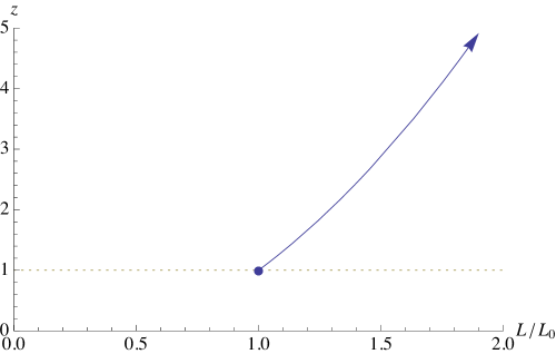
Figure 1: The flow of $(L,z)$ for a pure Schwarzschild-AdS₄ background. The arrow points towards the IR (i.e. decreasing values of $r$), and the dotted line highlights the AdS value $z=1$.

It is interesting to note that, while the relativistic $c$-theorem implies that $L$ is monotonically decreasing along flows to the IR, the Schwarzschild-AdS solution instead has an increasing flow to the IR, as shown in Fig. 1. Since there is no matter, this flow saturates the inequalities (20) and (21) implied by the null energy condition. In fact, this first inequality, $L^{\prime}\geq-(z-1)$, suggests that whenever $z>1$ (which is the usual Lifshitz case), the flow of $L$ tends to increase towards the IR. In order for $L$ to decrease, the bulk matter must contribute enough energy density to overcome the pull from the critical exponent. This balance between tendency towards non-extremality versus added matter must be resolved in order to flow to a stable IR fixed point. When this is done, as we will see below, flows can then occur in directions of both increasing and decreasing $L$.

III.2 Asymptotically Lifshitz black holes

For actual examples of black holes in an asymptotically Lifshitz spacetime, we may consider the model of Kachru:2008yh , or equivalently Taylor:2008tg . The latter formulation is given in terms of a massive vector field coupled to gravity

$$S=\frac{1}{2\kappa^{2}}\int d^{d+1}x\sqrt{-g}\left(R-V-{\textstyle\frac{1}{4}}F_{\mu\nu}F^{\mu\nu}-{\textstyle\frac{1}{2}}{m^{2}}A_{\mu}A^{\mu}\right).$$ (27)

Here $V$ and $m$ are constants parametrizing the model. This system admits Lifshitz backgrounds of the form (9), where $V$ and $m$ are related to $(L,z)$ by Taylor:2008tg ; Bertoldi:2009vn ; Braviner:2011kz

$$VL^{2}=-[z^{2}+(d-2)z+(d-1)^{2}],\qquad m^{2}L^{2}=(d-1)z,$$ (28)

and with the vector field

$$A=e^{zr/L}\sqrt{\frac{2(z-1)}{z}}dt.$$ (29)

Black hole flows of this system were considered in Bertoldi:2009vn , while flows between AdS and/or Lifshitz fixed points were considered in Kachru:2008yh ; Braviner:2011kz . The reason this simple model admits flows between Lifshitz fixed points is that the conditions (28) are invariant under the transformation

$$z\to\frac{(d-1)^{2}}{z},\qquad L\to(d-1)\frac{L}{z}.$$ (30)

Hence, for an appropriate set of parameters $V$ and $m$ [corresponding to $1\leq z\leq(d-1)^{2}$], the system admits two Lifshitz solutions along with vacuum AdS. As shown in Braviner:2011kz , a relevant deformation from the $z<d-1$ Lifshitz branch can cause a flow to either the $z>d-1$ Lifshitz branch or AdS in the IR.

As an example of the different possible holographic flows in this model, consider a four-dimensional bulk with $VL_{0}^{2}=-64/9$ and $m^{2}L_{0}^{2}=8/3$. These quantities are chosen so that the system admits two Lifshitz fixed points according to (28) in addition to a vacuum AdS fixed point:

$$(L,z)=(\sqrt{27/32}L_{0},1),\qquad(L,z)=(L_{0},4/3),\qquad(L,z)=(3L_{0}/2,3).$$ (31)

Starting at $z=4/3$ in the UV, this background can flow to either $z=1$ or $z=3$ in the IR Braviner:2011kz . The $z=1$ fixed point is of course an AdS bulk, which in turn can be deformed into Schwarzschild-AdS. Similarly, the $z=3$ Lifshitz background admits a black hole Bertoldi:2009vn with a regular horizon, and with the massive vector field vanishing at the horizon. These flows are shown in Fig. 2.

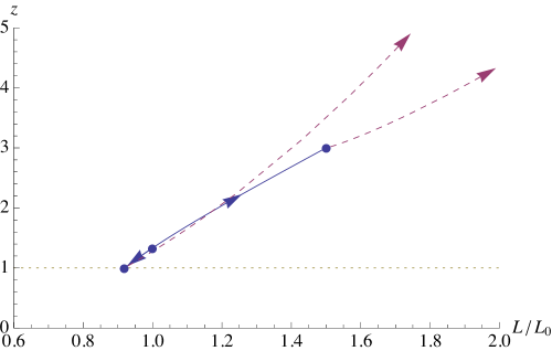
Figure 2: The flow of $(L,z)$ for the massive vector model with four bulk dimensions and with fixed points at $z=1$ (AdS), $z=4/3$ and $z=3$. The solid line flows connect fixed points, while the dashed lines correspond to $z=1$ (Schwarzschild-AdS) and $z=3$ black hole solutions.

What this example demonstrates is that flows between fixed points can proceed in either direction of increasing and decreasing $L$ and $z$. For $z\approx 1$, the two inequalities (20) and (21) favor flows where both $L$ and $z$ are decreasing towards the IR, as in the flow from Lifshitz to AdS. However, for $z>1$, the right hand sides of the inequalities are negative, and there is plenty of room for flows in the opposite direction, as evidenced by the flow to $z=3$ in the IR.

In this simple example of Lifshitz backgrounds supported by a massive vector field, the fixed point criteria (28) restricts the critical values of $(L,z)$ to lie on the curve

$$z=\left(\frac{m^{2}}{d-1}\right)L^{2}.$$ (32)

As a result, flows connecting two Lifshitz fixed points in this model always proceed from smaller $(L,z)$ in the UV to larger $(L,z)$ in the IR. In particular, both $L$ and $z$ necessarily flow in the same direction. In order to examine more general Lifshitz flows, we will need to decouple the fixed point values of $L$ and $z$. One way to do this is to introduce a variable effective mass for the vector field by introducing a scalar coupling. This is what we will do in the next section.

IV Lifshitz flows in a phenomenological model

As we have seen above, flows between Lifshitz fixed points can have a very rich structure, and do not appear to be strongly constrained by the null energy condition. Flows can also occur between AdS and Lifshitz fixed points, and between different AdS solutions, as shown in Braviner:2011kz in the context of six-dimensional $\mathcal{N}=(1,1)$ gauged supergravity and its consistent truncation. The advantage of working in the context of supergravity is that it naturally provides a stringy context for the bulk dual. However, the details of the full supergravity may at times obscure the key features of the flows. Thus we turn to a phenomenological model that nevertheless allows for a wide range of possibilities.

In order to examine holographic flows between unrelated fixed points, we extend the massive vector model of Kachru:2008yh ; Taylor:2008tg by adding a real scalar $\phi$, so that the bulk action takes the form

$$S=\frac{1}{2\kappa^{2}}\int d^{d+1}x\sqrt{-g}\left(R-{\textstyle\frac{1}{2}}\partial_{\mu}\phi\partial^{\mu}\phi-{\textstyle\frac{1}{4}}F_{\mu\nu}F^{\mu\nu}-V(\phi)-W(\phi)A_{\mu}A^{\mu}\right).$$ (33)

For the moment, we leave the potential $V(\phi)$ and scalar coupling $W(\phi)$ arbitrary, although we assume $\phi$ approaches a constant, $\phi(r)=\phi_{0}$, at fixed points of the flow. At such points, this system effectively reduces to (27) with $V=V(\phi_{0})$ and $m^{2}=2W(\phi_{0})$. The fixed point values of $(L,z)$ can then be extracted by inverting (28).

We proceed by making a domain wall ansatz

$$ds_{d+1}^{2}=-e^{2A(r)}dt^{2}+e^{2B(r)}d\vec{x}_{d-1}^{2}+dr^{2},{}$$

$$A=e^{G(r)}dt,\qquad\phi=\phi(r).$$ (34)

The action (33) gives rise to four dynamical equations

$$0 = (d-1)[B^{\prime\prime}+B^{\prime}(B^{\prime}-A^{\prime})]+{\textstyle\frac{1}{2}}\phi^{\prime 2}+e^{-2A+2G}W(\phi),{}$$

$$0 = A^{\prime\prime}+(d-2)B^{\prime\prime}+A^{\prime}(A^{\prime}-B^{\prime})+{\textstyle\frac{1}{2}}\phi^{\prime 2}-{\textstyle\frac{1}{2}}e^{-2A+2G}G^{\prime 2},{}$$

$$0 = G^{\prime\prime}+G^{\prime}\left[G^{\prime}-A^{\prime}+(d-1)B^{\prime}\right]-2W(\phi),{}$$

$$0 = \phi^{\prime\prime}+\phi^{\prime}\left[A^{\prime}+(d-1)B^{\prime}\right]-\partial V/\partial\phi+e^{-2A+2G}\partial W/\partial\phi,$$ (35)

along with one constraint

$$(d-1)B^{\prime}[2A^{\prime}+(d-2)B^{\prime}]+{\textstyle\frac{1}{2}}e^{-2A+2G}G^{\prime 2}-e^{-2A+2G}W(\phi)-{\textstyle\frac{1}{2}}\phi^{\prime 2}+V(\phi)=0.$$ (36)

The exponential factors $e^{-2A+2G}$ are associated with contractions of the vector potential, and may be removed by defining

$$H(r)\equiv e^{-A(r)+G(r)}.$$ (37)

Note that $H(r)$ is simply the time component of the vector field in the natural vielbein basis.

In order to focus on holographic RG flows, we may replace the metric functions $A$ and $B$ by the effective $L$ and $z$ functions given by (14). With this substitution, we obtain the equations for $(L,z,\phi,H)$

$$L^{\prime} = -(z-1)+\frac{L^{2}}{2(d-1)}(\phi^{\prime 2}+2W(\phi)H^{2}),{}$$

$$z^{\prime} = -\frac{(z-1)(2z+d-2)}{L}+\frac{L}{2}\left[\frac{z-1}{d-1}\phi^{\prime 2}+\left(H^{\prime}+\frac{z}{L}H\right)^{2}+\frac{z+d-2}{d-1}2W(\phi)H^{2}\right],{}$$

$$\phi^{\prime\prime} = -\frac{z+d-1}{L}\phi^{\prime}+\frac{\partial V}{\partial\phi}-\frac{\partial W}{\partial\phi}H^{2},{}$$

$$H^{\prime\prime} = -\frac{z+d-1}{L}H^{\prime}-\left[\left(\frac{z}{L}\right)^{\prime}+\frac{(d-1)z}{L^{2}}\right]H+2W(\phi)H.$$ (38)

In these variables, the constraint equation becomes

$$V(\phi)-W(\phi)H^{2}-\frac{1}{2}\phi^{\prime 2}+\frac{1}{2}\left(H^{\prime}+\frac{z}{L}H\right)^{2}+\frac{(d-1)(2z+d-2)}{L^{2}}=0.$$ (39)

At this point, it is worth pointing out that the first terms on the right hand sides of the $L^{\prime}$ and $z^{\prime}$ equations saturate the null energy condition inequalities (20) and (21), as they originate from the gravitational sector. The additional terms on the right hand side arise from the matter sector, and will contribute positively provided $z\geq 1$ [as already noted in (21)] and $W(\phi)\geq 0$. This latter condition on $W(\phi)$ is a direct consequence of the null energy condition.

IV.1 Lifshitz fixed points

Before proceeding to flows, we examine fixed points of this model where $(L,z,\phi,H)$ are all constant

$$(L,z,\phi,H)\to(L_{0},z_{0},\phi_{0},H_{0}).$$ (40)

Substituting these constant values into the equations of motion (38) and the constraint equation (39) gives two classes of solutions. The first has vanishing vector potential, $H_{0}=0$, and hence yields an AdS solution with $z_{0}=1$ and the AdS radius $L_{0}$ related to the critical value of the potential in the usual manner

$$z_{0}=1,\qquad V(\phi_{0})=-d(d-1)/L_{0}^{2},\qquad\partial_{\phi}V(\phi_{0})=0,\qquad H_{0}=0.$$ (41)

The second class is of Lifshitz form with

$$V(\phi_{0})L_{0}^{2} = -[z_{0}^{2}+(d-2)z_{0}+(d-1)^{2}],{}$$

$$2W(\phi_{0})L_{0}^{2} = (d-1)z_{0},{}$$

$$H_{0}^{2} = \frac{2(z_{0}-1)}{z_{0}},{}$$

$$\partial_{\phi}V(\phi_{0}) = \frac{2(z_{0}-1)}{z_{0}}\partial_{\phi}W(\phi_{0}).$$ (42)

Note that the first two expressions map directly onto (28), while the value of $H_{0}^{2}$ corresponds to (29). The final expression in (42) simply ensures that the scalar is at a critical point of its effective potential (which includes its coupling to the background vector).

Flows between fixed points may be generated by perturbing by a relevant deformation. In order to examine what deformations are allowed, we perform a linear stability analysis around a given Lifshitz fixed point specified by $(L_{0},z_{0},\phi_{0},H_{0})$. To do so, we first rewrite the equations of motion (38) in first order form by splitting the second order equations for $\phi$ and $H$ into pairs of equations for $(\phi,\phi^{\prime})$ and $(H,H^{\prime})$, respectively. We then perturb around the Lifshitz fixed point by taking

$$L = L_{0}+\epsilon\hat{L},\qquad\phi=\phi_{0}+\epsilon\hat{\phi},\qquad H=H_{0}+\epsilon\hat{H},{}$$

$$z = z_{0}+\epsilon\hat{z},\kern 22.0pt\phi^{\prime}=\epsilon\hat{\phi^{\prime}},\kern 37.00002ptH^{\prime}=\epsilon\hat{H^{\prime}}.$$ (43)

For $\epsilon\ll 1$, the linearized equations of motion reduce to $\mathcal{V}^{\prime}=\mathcal{M}\mathcal{V}$, where

$$\mathcal{V}=\{\hat{L},\hat{z},\hat{\phi},\hat{\phi^{\prime}},\hat{H},\hat{H^{\prime}}\}^{T},$$ (44)

and

$$\mathcal{M}=\begin{pmatrix}\frac{2(z_{0}-1)}{L_{0}}&-1&\frac{L_{0}^{2}}{d-1}H_{0}^{2}W_{1}&0&z_{0}H_{0}&0\\ \frac{2(z_{0}-1)(z_{0}+d-2)}{L_{0}^{2}}&-\frac{z_{0}+d-1}{L_{0}}&\frac{(z_{0}+d-2)L_{0}}{d-1}H_{0}^{2}W_{1}&0&\frac{2z_{0}+d-2}{L_{0}}z_{0}H_{0}&z_{0}H_{0}\\ 0&0&0&1&0&0\\ 0&0&V_{2}-H_{0}^{2}W_{2}&-\frac{z_{0}+d-1}{L_{0}}&-2H_{0}W_{1}&0\\ 0&0&0&0&0&1\\ \frac{2(z_{0}+d-2)}{L_{0}^{3}}H_{0}&0&\frac{z_{0}+d-2}{(z_{0}-1)(d-1)}H_{0}^{3}W_{1}&0&-\frac{2(z_{0}-1)(z_{0}+d-2)}{L_{0}^{2}}&-\frac{3z_{0}+d-3}{L_{0}}\end{pmatrix}.$$ (45)

Here we have expanded the potential $V(\phi)$ and scalar coupling $W(\phi)$ about the critical value $\phi_{0}$:

$$V(\phi) = V_{0}+V_{1}(\phi-\phi_{0})+{\textstyle\frac{1}{2}}V_{2}(\phi-\phi_{0})^{2}+\cdots,$$

$$W(\phi) = W_{0}+W_{1}(\phi-\phi_{0})+{\textstyle\frac{1}{2}}W_{2}(\phi-\phi_{0})^{2}+\cdots.$$ (46)

At this point, it is worth summarizing the various parameters that enter into the matrix $\mathcal{M}$. The critical point determined by (42) may be thought of as having particular values of the Lifshitz parameters $(L_{0},z_{0})$. Then, at this fixed point, the constant values of $V(\phi_{0})$ and $W(\phi_{0})$ become

$$V_{0}=-\frac{z_{0}^{2}+(d-2)z_{0}+(d-1)^{2}}{L_{0}^{2}},\qquad W_{0}=\frac{(d-1)z_{0}}{2L_{0}^{2}}.$$ (47)

These quantities, however, do not directly enter into $\mathcal{M}$. The linear terms in (46) are constrained by the last condition in (42)

$$V_{1}=H_{0}^{2}W_{1},\qquad\mbox{where}\qquad H_{0}^{2}=\frac{2(z_{0}-1)}{z_{0}}.$$ (48)

Since $H_{0}$ is determined in terms of $z_{0}$, it cannot considered a free parameter. As a result, the linearized behavior at a Lifshitz fixed point depends only on the values of $(L_{0},z_{0})$, the linear potential parameter $W_{1}$ (or equivalently $V_{1}$) and the quadratic potential parameters $V_{2}$ and $W_{2}$.

The solution to the first order equation $\mathcal{V}^{\prime}=\mathcal{M}\mathcal{V}$ is given by

$$\mathcal{V}(r)=\sum_{i}\mathcal{V}_{i}e^{\lambda_{i}r},$$ (49)

where $\{\lambda_{i}\}$ are the eigenvalues of $\mathcal{M}$, with corresponding eigenvectors $\{\mathcal{V}_{i}\}$. Since we assume the asymptotic form of the metric (9), where $r\to\infty$ corresponds to the UV, relevant deformations (which induce a flow to the IR) will correspond to negative eigenvalues, namely $\lambda^{\rm(UV)}_{i}<0$. If this flow terminates at a stable IR fixed point, then it will necessarily approach the IR fixed point along a direction or set of directions with positive eigenvalues, $\lambda^{\rm(IR)}_{i}>0$.

The eigenvalues of $\mathcal{M}$ are easily determined, although their general expressions are not particularly illuminating. Much of the complication arises when the linear term is non-vanishing (i.e. when $W_{1}\neq 0$), as in this case the scalar and vector fluctuations no longer decouple at fixed points. We therefore restrict the presentation of explicit results to the case when $W_{1}=0$. In this case, there is a single marginal mode, $\lambda_{1}=0$, with eigenvector

$$\mathcal{V}_{1}=\left(H_{0}L_{0},2z_{0}H_{0},0,0,\frac{2}{z_{0}},0\right).$$ (50)

This marginal direction corresponds to holding $\phi$ fixed, and moving along the curve given by $2W_{0}L_{0}^{2}=(d-1)z_{0}$ in (42). Note, however, that while this deformation is marginal in the set of first order equations, movement along this direction will not satisfy the constraint (39). Thus this mode takes us outside of a given model, and in particular shifts the vacuum energy $V_{0}$ (which is a constant of integration of the set of first order equations).

There are three additional modes that keep $\phi$ fixed, but involve a combination of the metric and vector field. The first one of this set is always relevant, with $\lambda_{2}=-(z_{0}+d-1)/L_{0}$ and eigenvector

$$\mathcal{V}_{2}=\left(\frac{H_{0}L_{0}}{z_{0}+d-2},\frac{z_{0}-d+1}{z_{0}+d-2}H_{0},0,0,-\frac{2}{z_{0}},\frac{2(z_{0}+d-1)}{z_{0}L_{0}}\right).$$ (51)

The other two are paired up, with

$$\lambda_{3,4}=-\frac{z_{0}+d-1}{2L_{0}}(1\pm\Delta),$$ (52)

and

$$\mathcal{V}_{3,4} = \biggl{(}\frac{2-4z_{0}+(z_{0}+d-1)(1\mp\Delta)}{2(z_{0}+d-2)}H_{0}L_{0},\frac{-4z_{0}+(z_{0}+d-1)(1\mp\Delta)}{2}H_{0},$$ (53)

$$\qquad 0,0,-\frac{2}{z_{0}},\frac{(z_{0}+d-1)(1\mp\Delta)}{z_{0}L_{0}}\biggr{)},$$

where

$$\Delta=\sqrt{1+\frac{8(z_{0}-1)(z_{0}-d+1)}{(z_{0}+d-1)^{2}}}.$$ (54)

Since we take $\Delta$ to be positive, $\lambda_{3}$ [corresponding to the top sign in (52)] will always be negative, corresponding to a relevant deformation. However, the behavior of $\lambda_{4}$ depends on the value of $\Delta$. For $1\leq z_{0}\leq d-1$, we find $\Delta\leq 1$, so that $\lambda_{4}\leq 0$. On the other hand, we obtain an irrelevant deformation, $\lambda_{4}>0$, whenever $z_{0}>d-1$.

The remaining two modes only involve the scalar field $\phi$ and its derivative (in the linearized analysis), and have eigenvalues

$$\lambda_{5,6}=-\frac{z_{0}+d-1}{2L_{0}}(1\pm\Sigma),$$ (55)

along with eigenvectors

$$\mathcal{V}_{5,6}=\left(0,0,\frac{(z_{0}+d-1)(1\mp\Sigma)}{2L_{0}},V_{2}-H_{0}^{2}W_{2},0,0\right),$$ (56)

where

$$\Sigma=\sqrt{1+\frac{4L_{0}^{2}(V_{2}-H_{0}^{2}W_{2})}{(z_{0}+d-1)^{2}}}.$$ (57)

Since we are assuming the absence of linear terms in $V(\phi)$ and $W(\phi)$ at the critical point, it is clear that the combination $m_{0,\rm eff}^{2}\equiv V_{2}-H_{0}^{2}W_{2}$ is simply the effective mass of $\phi$. Note that, in the AdS case when $z_{0}=1$, we find the expected relation between scalar mass and conformal dimension

$$\lambda_{5,6}=-\frac{1}{L_{0}}\left(d/2\pm\sqrt{(d/2)^{2}+m_{0,\rm eff}^{2}L_{0}^{2}}\right)\qquad(\mbox{for }z_{0}=1).$$ (58)

The only modification for general $z_{0}$ is then the replacement $d\to z_{0}+d-1$. The behavior of $\lambda_{5,6}$ depends on the sign of $m_{0,\rm eff}^{2}$. For $-[(z_{0}+d-1)/2L_{0}]^{2}\leq m_{0,\rm eff}^{2}\leq 0$ (where the lower bound is taken as a generalization of the Breitenlohner-Freedman bound Breitenlohner:1982bm ; Breitenlohner:1982jf ), both $\lambda_{5}$ and $\lambda_{6}$ are negative, so the scalar deformations are both relevant. However, for $m_{0,\rm eff}^{2}>0$, one of the deformations becomes irrelevant, corresponding to $\lambda_{6}>0$.

In summary, after linearizing about a Lifshitz fixed point, we find a set of six perturbations, of which one is marginal. (This remains the case even when $W_{1}\neq 0$.) However, this marginal direction is to be disregarded, as it is eliminated by the constraint (39). Of the remaining five modes, three are always relevant, while the other two will depend on the parameters of the fixed point. In the absence of a linear coupling, the modes become irrelevant in the following cases:

$$\lambda_{4}>0, \text{when}\quad z_{0}>d-1,$$ (59)

$$\lambda_{6}>0, \text{when}\quad m_{0,\rm eff}^{2}\equiv V_{2}-H_{0}^{2}W_{2}>0.$$ (60)

Since $\mathcal{V}_{2,3,4}$ have vanishing components along $\hat{\phi}$ and $\hat{\phi}^{\prime}$, we label the flows induced by these modes as “vector field driven”. On the other hand, since $\mathcal{V}_{5,6}$ initiates flows along $\hat{\phi}$ and $\hat{\phi}^{\prime}$, we will label such flows as “scalar field driven”.

IV.2 AdS fixed points

Although our main interest is to examine Lifshitz fixed points, the simple model (33) also admits AdS fixed points given by (41). The stability analysis of such fixed points is similar to that of Lifshitz fixed points. However, we cannot simply set $z_{0}=1$ in the previous results, as the second condition in (42) is no longer applicable when the massive vector is turned off. Nevertheless, the deformations can be classified in essentially the same manner.

Again, there is a single marginal mode with $\lambda_{1}=0$ and

$$\mathcal{V}_{1}=(1,0,0,0,0,0).$$ (61)

This marginal direction corresponds to shifting the cosmological constant, and is again removed by the constraint (39). The three modes found above involving the metric and vector field now split into a relevant metric deformation with $\lambda_{2}=-d/L_{0}$ and

$$\mathcal{V}_{2}=(L_{0},d,0,0,0,0),$$ (62)

and a pair of vector field deformations with

$$\lambda_{3,4}=-\frac{d\pm\sqrt{(d-2)^{2}+8W_{0}L_{0}^{2}}}{2L_{0}}$$ (63)

and

$$\mathcal{V}_{3,4}=\left(0,0,0,0,-1,\frac{d\pm\sqrt{(d-2)^{2}+8W_{0}L_{0}^{2}}}{2L_{0}}\right).$$ (64)

The metric deformation generates a flow to a Schwarzschild-AdS black hole, while the two vector field modes have the expected conformal dimensions for a massive vector in AdS with an effective mass of $m_{1,\rm eff}^{2}=2W_{0}$. (Recall that the null energy condition demands $W(\phi)\geq 0$, so that $m_{1,\rm eff}^{2}$ must be non-negative.) For $0\leq m_{1,\rm eff}^{2}\leq(d-1)/L_{0}^{2}$, both vector modes are relevant, while for $m_{1,\rm eff}^{2}>(d-1)/L_{0}^{2}$, the deformation corresponding to $\lambda_{4}$ becomes irrelevant.

Finally, the remaining two modes are those of the scalar field, with

$$\lambda_{5,6}=-\frac{1}{L_{0}}\left(d/2\pm\sqrt{(d/2)^{2}+V_{2}L_{0}^{2}}\right),$$ (65)

and

$$\mathcal{V}_{5,6}=\left(0,0,\frac{d/2\mp\sqrt{(d/2)^{2}+V_{2}L_{0}^{2}}}{L_{0}},V_{2},0,0\right),$$ (66)

in agreement with (58), where $m_{0,\rm eff}^{2}=V_{2}$ is just the scalar mass read off from the potential. As a result, we find that the deformations away from an AdS fixed point are all relevant, except for the two cases

$$\lambda_{4}>0, \text{when}\quad m_{1,\rm eff}^{2}\equiv 2W_{0}>(d-1)/L_{0}^{2},$$ (67)

$$\lambda_{6}>0, \text{when}\quad m_{0,\rm eff}^{2}\equiv V_{2}>0,$$ (68)

where the corresponding deformations become irrelevant. As above, flows to or from AdS fixed points may be thought of as either vector field driven or scalar field driven. Of course, since the vector field vanishes at AdS fixed points, a scalar field deformation may initiate a flow between AdS fixed points, but would not otherwise generate a non-vanishing vector field background. Such scalar field driven flows will thus maintain $z=1$ throughout the flow, unless accompanied by a metric or vector perturbation.

IV.3 Flows between fixed points

With the linear stability analysis out of the way, we now consider flows between fixed points. Such flows may be generated by starting at a UV fixed point $(L_{\rm UV},z_{\rm UV})$, and turning on a relevant deformation. This model admits five deformations away from any fixed point, of which three are always relevant. Hence it is always possible to construct a flow away from the UV. However, not all such flows will terminate in an IR fixed point. We find that generic deformations will flow to a singularity with both the scalar and vector fields running away to infinity. Furthermore, as discussed previously, flows to a black hole horizon are also possible.

Assuming, however, that the flow reaches an IR fixed point with $(L_{\rm IR},z_{\rm IR})$, it will approach this fixed point in an irrelevant direction. For a Lifshitz fixed point (assuming vanishing linear $\phi$ coupling at this point), the criteria for an irrelevant deformation are given by either (59), which requires $z_{\rm IR}>d-1$, or (60), which requires $m_{0,\rm IR}^{2}>0$. The former corresponds to a vector field driven flow, while the latter corresponds to a scalar field driven flow. For an AdS fixed point in the IR, the first criterion is replaced by (67), which requires $m_{1,\rm IR}^{2}>(d-1)/L_{\rm IR}^{2}$.

At this point, it is worth noting that the flows of Kachru:2008yh ; Braviner:2011kz in the massive vector model are naturally vector field driven, as this model lacks the extra scalar. In this case, Lifshitz fixed points in the IR must lie in the $z_{\rm IR}>d-1$ branch, as can be seen in the example of Fig. 2. Similarly, it can be seen that AdS fixed points in the IR can be reached for flows starting with $1<z_{\rm UV}<(d-1)^{2}$.

In the absence of a specific model, we forego a general analysis of flows between fixed points. However, it is instructive to provide a few examples of scalar field driven Lifshitz to Lifshitz flows. In particular, we may engineer such flows by choosing appropriate forms of the scalar potential $V(\phi)$ and vector field coupling $W(\phi)$. A natural, and fairly minimal choice would be to construct the potential $V$ to have two critical points, corresponding to the UV and IR. We then design $W$ so that the effective vector mass, $m_{1,\rm eff}^{2}$, takes on appropriate values at the critical points, so as to yield the desired Lifshitz scaling according to (47). Although it is possible to choose a linear function for $W$, for simplicity we demand that both $V$ and $W$ have critical points at the same values of $\phi$. This allows us to avoid any linear shift in the potential implied by (48).

The simplest model with two critical points involves taking cubic potentials

$$V(\phi) = V_{0}+V_{1}\phi+V_{2}\phi^{2}+V_{3}\phi^{3},$$

$$W(\phi) = W_{0}+W_{1}\phi+W_{2}\phi^{2}+W_{3}\phi^{3}.$$ (69)

Although a cubic $W(\phi)$ will always become negative in some domain, we will always restrict $\phi$ so that $W(\phi)\geq 0$ to ensure compatibility with the null energy condition. This is a legitimate restriction since we are only interested in classical solutions to the equations of motion. The eight constants of the potentials are fixed by demanding that they admit an IR critical point at $\phi=0$ with $(L_{\rm IR},z_{\rm IR})$ and a UV critical point at $\phi=\phi_{0}$ with $(L_{\rm UV},z_{\rm UV})$. We find, in particular

$$V_{0} = -\frac{z_{\rm IR}^{2}+(d-2)z_{\rm IR}+(d-1)^{2}}{L_{\rm IR}^{2}},$$

$$V_{1} = 0,$$

$$V_{2}\phi_{0}^{2} = 3\left[\frac{z_{\rm IR}^{2}+(d-2)z_{\rm IR}+(d-1)^{2}}{L_{\rm IR}^{2}}-\frac{z_{\rm UV}^{2}+(d-2)z_{\rm UV}+(d-1)^{2}}{L_{\rm UV}^{2}}\right],$$

$$V_{3}\phi_{0}^{3} = -2\left[\frac{z_{\rm IR}^{2}+(d-2)z_{\rm IR}+(d-1)^{2}}{L_{\rm IR}^{2}}-\frac{z_{\rm UV}^{2}+(d-2)z_{\rm UV}+(d-1)^{2}}{L_{\rm UV}^{2}}\right],$$

and

$$W_{0} = \frac{(d-1)z_{\rm IR}}{2L_{\rm IR}^{2}},$$

$$W_{1} = 0,$$

$$W_{2}\phi_{0}^{2} = -\frac{3(d-1)}{2}\left[\frac{z_{\rm IR}}{L_{\rm IR}^{2}}-\frac{z_{\rm UV}}{L_{\rm UV}^{2}}\right],$$

$$W_{3}\phi_{0}^{3} = (d-1)\left[\frac{z_{\rm IR}}{L_{\rm IR}^{2}}-\frac{z_{\rm UV}}{L_{\rm UV}^{2}}\right].$$ (71)

It is worth noting, however, that this model does not necessarily admit a stable flow from arbitrary values of $(L_{\rm UV},z_{\rm UV})$ to $(L_{\rm IR},z_{\rm IR})$, as relevant deformations from the UV could often flow to a black hole or singular geometry. In addition, there is a two-fold degeneracy of fixed points (both at the UV and the IR), corresponding to the map given by (30). Hence flows could originate or terminate in the dual fixed points from the ones that were originally desired.

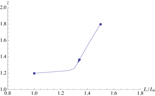
Figure 3: A scalar field driven flow with decreasing $z$ and $L$. We have taken $d=3$ and $\phi_{0}=1$, along with the fixed point parameters given in (72).

In order to go beyond the linearized analysis, we solve the equations of motion (38) numerically, integrating out from the IR to the UV along an irrelevant direction. The reason we integrate out from the IR is that, as indicated above, there are at most only two irrelevant deformations in the IR, given by the conditions (59) and (60). Since we are interested in scalar field driven flows (where $\phi$ flows between the UV and IR critical points of the potential), we naturally choose the $\lambda_{6}$ direction for the deformation. An example of a scalar field driven flow towards decreasing $z$ is shown in Fig. 3, where we have chosen a four-dimensional bulk and fixed point parameters

$$(L_{\rm UV},z_{\rm UV})=(3L_{0}/2,9/5),\qquad(L_{\rm IR},z_{\rm IR})=(L_{0},6/5).$$ (72)

Note that $z$ lies in the range $1\leq z\leq d-1$ for this class of flows. We see that there is some slight ringing as $\phi$ flows away from $\phi_{0}$ (where $V(\phi_{0})$ is a local maximum) in the UV.

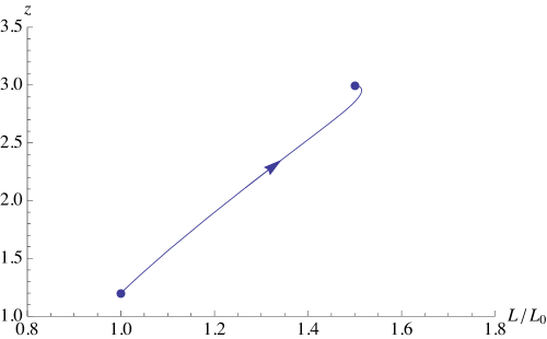
Figure 4: A scalar field driven flow with increasing $z$ and $L$. The fixed point parameters are given in (73), along with $d=3$ and $\phi_{0}=1$.

It is also easy to obtain flows towards increasing $z$. One such example is shown in Fig. 4, where the fixed point values are given by

$$(L_{\rm UV},z_{\rm UV})=(L_{0},6/5),\qquad(L_{\rm IR},z_{\rm IR})=(3L_{0}/2,3).$$ (73)

The general feature of this flow is similar to the vector field driven flow from $z=4/3$ to $z=3$ shown in Fig. 2. However, we note that the effective value of $L$ actually overshoots its IR fixed point value before finally turning around and reaching it at the end of the flow. This is a clear indication that the function $L(r)$ is not constrained to be monotonic by the null energy condition. It is not obvious whether this has any physical significance, as the effective $L$ and $z$ functions are not necessarily observable along the flow. It is also possible to obtain flows towards increasing $z$, but with decreasing $L$. An interesting example is given in Fig. 5, corresponding to

$$(L_{\rm UV},z_{\rm UV})=(3L_{0}/2,6/5),\qquad(L_{\rm IR},z_{\rm IR})=(L_{0},9/5).$$ (74)

Here we see that the effective values of both $L$ and $z$ flow away from the UV for some distance before turning around and reaching the IR fixed point. The ringing near the UV fixed point of the potential is also more pronounced, as both the scalar and vector fields participate in the flow.

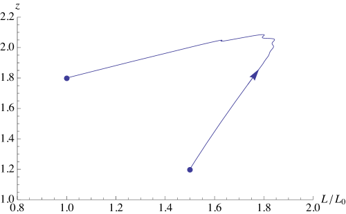
Figure 5: A scalar field driven flow with increasing $z$ and decreasing $L$. We have taken $d=3$ and $\phi_{0}=1$, along with the parameters given in (74).

V Discussion

In the relativistic case ($z=1$), the consequence of the null energy condition directly leads to the holographic $c$-theorem, $L^{\prime}\geq 0$. However, once relativistic invariance is no longer required, the implications of the null energy condition are very much relaxed. Although it is possible to define two monotonic functions, $C_{1}$ and $C_{2}$, as in (17), neither one of them serves the purpose of a useful $c$-function, as they do not approach constant values at fixed points (except when $z=1$, in which case $C_{1}$ coincides with the usual holographic $c$-function).

For a Lifshitz fixed point, the more useful quantities $(L,z)$ do not exhibit any obvious monotonicity. Using a cubic potential model, we have constructed flows between two Lifshitz fixed points that satisfy the null energy condition, and where $L$ and $z$ are simultaneously increasing or decreasing or where $L$ is decreasing while $z$ is increasing. So far, however, we have been unable to find any examples of flows with simultaneously decreasing $z$ and increasing $L$. It is possible that this is a feature of the toy model, as the null energy condition in itself does not preclude such flows. Nevertheless, the inequalities (17) obviously place some restraints on the allowed flows, and it would be interesting to see whether there is a deeper reason why we have not found any flows where $z$ decreases while $L$ increases.

Although we have focused on flows between scale invariant Lifshitz fixed points, there has been recent interest in systems involving hyperscaling violation (parametrized by $\theta$) in addition to the dynamical critical exponent $z$. Gravitational duals to such models have been realized in Einstein-Maxwell-dilaton theories Gubser:2009qt ; Charmousis:2010zz ; Perlmutter:2010qu , and aspects of the null energy condition have been investigated in Ogawa:2011bz ; Huijse:2011ef ; Dong:2012se . Metrics exhibiting hyperscaling violation may be written in the conformally Lifshitz form

$$ds_{d+1}^{2}=r^{2\theta/(d-1)}\left[-\frac{dt^{2}}{r^{2z}}+\frac{d\vec{x}_{d-1}^{\,2}+dr^{2}}{r^{2}}\right].$$ (75)

In order to make contact with (11), we transform $r\to r^{(d-1)/\theta}$ (and rescale the coordinates) so that

$$ds_{d+1}^{2}=-r^{2(1-z(d-1)/\theta)}dt^{2}+r^{2(1-(d-1)/\theta)}d\vec{x}_{d-1}^{\,2}+dr^{2}.$$ (76)

Therefore, in a hyperscaling region, we make the identification

$$A(r)=\left(1-\frac{z(d-1)}{\theta}\right)\log r,\qquad B(r)=\left(1-\frac{(d-1)}{\theta}\right)\log r.$$ (77)

This may be contrasted with the behavior $A\sim zr/L$ and $B\sim r/L$ in the case where $\theta=0$. (Note, however, that this identification is not well-behaved in the limit $\theta\to 0$, as the scale-invariant metric functions behave as exponentials and not power-laws.)

It is interesting to see what the flow functions $L(r)$ and $z(r)$ defined in (14) look like for the metric (76). We find

$$L(r)=-\frac{\theta}{d-1-\theta}r,\qquad z(r)=1+\frac{(z-1)(d-1)}{d-1-\theta},$$ (78)

where we should keep in mind that $z(r)$ is an effective function that was designed to match the critical exponent only at pure Lifshitz fixed points, while $z$ is the true critical exponent given in (76). By construction, $z(r)$ and $z$ coincide in the absence of hyperscaling violation (i.e. when $\theta=0$). However, the effective function $L(r)$ runs linearly in $r$, and hence cannot be assigned a fixed value in a hyperscaling region of any flow.

For $L(r)$ and $z(r)$ given in (78), the null energy condition (19) gives rise to the inequalities

$$(d-1-\theta)((z-1)(d-1)-\theta)\geq 0,\qquad(z-1)(z+d-1-\theta)\geq 0,$$ (79)

as noted in Dong:2012se . It would be interesting to see whether these conditions can be extended along a complete flow between regions with different scaling behavior. Of course, the two functions $C_{1}(r)$ and $C_{2}(r)$ in (17) are valid $c$-functions regardless of the geometry. However, the usefulness of the functions depend on being able to express them in terms of ‘physical’ quantities such as $\theta$ and $z$ at fixed points of the flow. We have, unfortunately, not been able to find a suitable set of $\theta(r)$ and $z(r)$ functions that extend the behavior of (77) beyond the fixed points. The main obstacle in doing so is to properly reproduce the power-law behavior implicit in the $\log r$ running of $A(r)$ and $B(r)$.

A possible attempt at defining a $c$-function for flows with hyperscaling violation is to capture the power-law behavior $e^{A}\sim r^{\alpha}$ by removing the explicit $r$ dependence in (77). This may be done by forming ratios, such as $(A^{\prime})^{2}/A^{\prime\prime}$, $(B^{\prime})^{2}/B^{\prime\prime}$ or $A^{\prime}/B^{\prime}$. For example, we may define

$$z(r)\equiv\frac{B^{\prime\prime}+A^{\prime}B^{\prime}}{B^{\prime\prime}+(B^{\prime})^{2}},\qquad\theta(r)\equiv(d-1)\frac{B^{\prime\prime}}{B^{\prime\prime}+(B^{\prime})^{2}},$$ (80)

so that $z(r)$ and $\theta(r)$ approach the constant values $z_{0}$ and $\theta_{0}$ at fixed points of the flow. This extension of $z$ and $\theta$ away from fixed points is not unique, but has the advantage that the first inequality in (16) yields simply

$$(d-1-\theta(r))((z(r)-1)(d-1)-\theta(r))\geq 0,$$ (81)

which is identical in form to the first equation in (79), but now must hold everywhere along the flow. Unfortunately, the second inequality in (16) does not have a simple expression in terms of $z(r)$ and $\theta(r)$ because $A^{\prime\prime}$ in (16) has no natural counterpart in the definition (80). Note, also, that the inequality (81) does not take the conventional form of a gradient of a $c$-function, and hence does not suggest any direction for the flow of $z$ or $\theta$. Nevertheless, this discussion suggests that additional information may be captured from the null energy condition beyond just the fixed point inequalities (79).

Finally, once again ignoring hyperscaling violation, we note that it may be possible to resolve the tidal singularity at the Lifshitz horizon by flowing into AdS${}_{2}\times\mathbb{R}^{d-1}$ in the deep IR Harrison:2012vy . Since the AdS${}_{2}\times\mathbb{R}^{d-1}$ geometry is obtained by taking $B(r)=0$ in (11), the definition of the flow functions $L(r)$ and $z(r)$ in (14) break down in this case. In particular, the flow to AdS${}_{2}\times\mathbb{R}^{d-1}$ is represented by

$$L(r)\to\infty,\qquad z(r)\to\infty,\qquad\mbox{with $z(r)/L(r)=L_{2}$ held fixed},$$ (82)

where $L_{2}$ is the radius of the emergent AdS₂. Note that this is distinct from the Schwarzschild black hole flows shown in Figs. 1 and 2, as the Schwarzschild flows have $z(r)\sim L^{2}(r)\to\infty$ as the flow approaches the black hole horizon.

Regardless of the nature of the model, as long as it is a two-derivative theory of gravity, the power of the null energy condition is that it directly translates to a condition on the geometry, (3), and hence a condition on its geodesics and causal structure. Although there has been progress in understanding the implications of the null energy condition for higher derivative gravity, once additional terms enter the left-hand side of the Einstein equation, the null energy condition by itself no longer completely determines the Ricci tensor. As a result, additional conditions may be required in the gravitational sector in order to have a well-behaved holographic dual. It would be worthwhile to extend our results for holographic Lifshitz flows to the case of higher derivative gravity in the bulk, and to investigate what form these additional conditions may take.

- (1) E. Alvarez and C. Gomez, Geometric holography, the renormalization group and the c theorem, Nucl. Phys. B 541, 441 (1999) [hep-th/9807226].
- (2) L. Girardello, M. Petrini, M. Porrati and A. Zaffaroni, Novel local CFT and exact results on perturbations of N=4 superYang Mills from AdS dynamics, JHEP 9812, 022 (1998) [hep-th/9810126].
- (3) D. Z. Freedman, S. S. Gubser, K. Pilch and N. P. Warner, Renormalization group flows from holography supersymmetry and a c theorem, Adv. Theor. Math. Phys. 3, 363 (1999) [hep-th/9904017].
- (4) V. Sahakian, Holography, a covariant c function, and the geometry of the renormalization group, Phys. Rev. D 62, 126011 (2000) [hep-th/9910099].
- (5) M. Henningson and K. Skenderis, The Holographic Weyl anomaly, JHEP 9807, 023 (1998) [hep-th/9806087].
- (6) M. Henningson and K. Skenderis, Holography and the Weyl Anomaly, Fortsch. Phys. 48 (2000) 125 [arXiv:hep-th/9812032].
- (7) A. B. Zamolodchikov, Irreversibility of the Flux of the Renormalization Group in a 2D Field Theory, JETP Lett. 43, 730 (1986) [Pisma Zh. Eksp. Teor. Fiz. 43, 565 (1986)].
- (8) Z. Komargodski and A. Schwimmer, On Renormalization Group Flows in Four Dimensions, JHEP 1112, 099 (2011) [arXiv:1107.3987 [hep-th]].
- (9) S. Gao and R. M. Wald, Theorems on gravitational time delay and related issues, Class. Quant. Grav. 17, 4999 (2000) [gr-qc/0007021].
- (10) R. V. Buniy and S. D. H. Hsu, Instabilities and the Null Energy Condition, Phys. Lett. B 632 (2006) 543 [arXiv:hep-th/0502203].
- (11) S. Dubovsky, T. Gregoire, A. Nicolis and R. Rattazzi, Null Energy Condition and Superluminal Propagation, JHEP 0603 (2006) 025 [arXiv:hep-th/0512260].
- (12) R. V. Buniy, S. D. H. Hsu and B. M. Murray, The Null Energy Condition and Instability, Phys. Rev. D 74 (2006) 063518 [arXiv:hep-th/0606091].
- (13) M. Kleban, J. McGreevy and S. D. Thomas, Implications of bulk causality for holography in AdS, JHEP 0403, 006 (2004) [hep-th/0112229].
- (14) A. Sinha, On the New Massive Gravity and AdS/CFT, JHEP 1006 (2010) 061 [arXiv:1003.0683 [hep-th]].
- (15) J. Oliva and S. Ray, A new cubic theory of gravity in five dimensions: Black hole, Birkhoff’s theorem and c-function, Class. Quant. Grav. 27, 225002 (2010) [arXiv:1003.4773 [gr-qc]].
- (16) R. C. Myers and A. Sinha, Seeing a c-Theorem with Holography, Phys. Rev. D 82 (2010) 046006 [arXiv:1006.1263 [hep-th]].
- (17) A. Sinha, On Higher Derivative Gravity, c-Theorems and Cosmology, Class. Quant. Grav. 28 (2011) 085002 [arXiv:1008.4315 [hep-th]].
- (18) R. C. Myers and A. Sinha, Holographic c-Theorems in Arbitrary Dimensions, JHEP 1101 (2011) 125 [arXiv:1011.5819 [hep-th]].
- (19) J. T. Liu, W. Sabra and Z. Zhao, Holographic c-theorems and higher derivative gravity, arXiv:1012.3382 [hep-th].
- (20) M. F. Paulos, Holographic phase space: -functions and black holes as renormalization group flows, JHEP 1105, 043 (2011) [arXiv:1101.5993 [hep-th]].
- (21) J. T. Liu and Z. Zhao, A holographic c-theorem for higher derivative gravity, arXiv:1108.5179 [hep-th].
- (22) S. A. Hartnoll, Lectures on holographic methods for condensed matter physics, Class. Quant. Grav. 26, 224002 (2009) [arXiv:0903.3246 [hep-th]].
- (23) C. P. Herzog, Lectures on Holographic Superfluidity and Superconductivity, J. Phys. A 42, 343001 (2009) [arXiv:0904.1975 [hep-th]].
- (24) J. McGreevy, Holographic duality with a view toward many-body physics, Adv. High Energy Phys. 2010, 723105 (2010) [arXiv:0909.0518 [hep-th]].
- (25) H. Braviner, R. Gregory and S. F. Ross, Flows involving Lifshitz solutions, Class. Quant. Grav. 28, 225028 (2011) [arXiv:1108.3067 [hep-th]].
- (26) C. Hoyos and P. Koroteev, On the Null Energy Condition and Causality in Lifshitz Holography, Phys. Rev. D 82, 084002 (2010) [Erratum-ibid. D 82, 109905 (2010)] [arXiv:1007.1428 [hep-th]].
- (27) S. Kachru, X. Liu and M. Mulligan, Gravity Duals of Lifshitz-like Fixed Points, Phys. Rev. D 78, 106005 (2008) [arXiv:0808.1725 [hep-th]].
- (28) M. Taylor, Non-relativistic holography, arXiv:0812.0530 [hep-th].
- (29) G. Bertoldi, B. A. Burrington and A. Peet, Black Holes in asymptotically Lifshitz spacetimes with arbitrary critical exponent, Phys. Rev. D 80, 126003 (2009) [arXiv:0905.3183 [hep-th]].
- (30) P. Breitenlohner and D. Z. Freedman, Positive Energy in anti-De Sitter Backgrounds and Gauged Extended Supergravity, Phys. Lett. B 115, 197 (1982).
- (31) P. Breitenlohner and D. Z. Freedman, Stability in Gauged Extended Supergravity, Annals Phys. 144, 249 (1982).
- (32) S. S. Gubser and F. D. Rocha, Peculiar properties of a charged dilatonic black hole in AdS5, Phys. Rev. D 81, 046001 (2010) [arXiv:0911.2898 [hep-th]].
- (33) C. Charmousis, B. Gouteraux, B. S. Kim, E. Kiritsis and R. Meyer, Effective Holographic Theories for low-temperature condensed matter systems, JHEP 1011, 151 (2010) [arXiv:1005.4690 [hep-th]].
- (34) E. Perlmutter, Domain Wall Holography for Finite Temperature Scaling Solutions, JHEP 1102, 013 (2011) [arXiv:1006.2124 [hep-th]].
- (35) N. Ogawa, T. Takayanagi and T. Ugajin, Holographic Fermi Surfaces and Entanglement Entropy, JHEP 1201, 125 (2012) [arXiv:1111.1023 [hep-th]].
- (36) L. Huijse, S. Sachdev and B. Swingle, Hidden Fermi surfaces in compressible states of gauge-gravity duality, Phys. Rev. B 85, 035121 (2012) [arXiv:1112.0573 [cond-mat.str-el]].
- (37) X. Dong, S. Harrison, S. Kachru, G. Torroba and H. Wang, Aspects of holography for theories with hyperscaling violation, arXiv:1201.1905 [hep-th].
- (38) S. Harrison, S. Kachru and H. Wang, Resolving Lifshitz Horizons, arXiv:1202.6635 [hep-th].