Light sterile neutrino production in the early universe with dynamical neutrino asymmetries

Abstract

Light sterile neutrinos mixing with the active ones have been recently proposed to solve different anomalies observed in short-baseline oscillation experiments. These neutrinos can also be produced by oscillations of the active neutrinos in the early universe, leaving possible traces on different cosmological observables. Here we perform an updated study of the neutrino kinetic equations in (3+1) and (2+1) oscillation schemes, dynamically evolving primordial asymmetries of active neutrinos and taking into account for the first time CP-violation effects. In the absence of neutrino asymmetries, eV-mass scale sterile neutrinos would be completely thermalized creating a tension with respect to the CMB, LSS and BBN data. In the past literature, active neutrino asymmetries have been invoked as a way to inhibit the sterile neutrino production via the in-medium suppression of the sterile-active mixing angle. However, neutrino asymmetries also permit a resonant sterile neutrino production. We find that if the active species have equal asymmetries $L$, a value $|L|=10^{-3}$ is required to start suppressing the resonant sterile production, roughly an order of magnitude larger than what previously expected. When active species have opposite asymmetries the sterile abundance is further enhanced, requiring an even larger $|L|\simeq 10^{-2}$ to start suppressing their production. In the latter case, CP-violation (naturally expected) further exacerbates the phenomenon. Some consequences for cosmological observables are briefly discussed: for example, it is likely that moderate suppressions of the sterile species production are associated with significant spectral distortions of the active neutrino species, with potentially interesting phenomenological consequences especially for BBN.

I Introduction

In recent years a renewed attention has been paid to light ($m\sim\mathcal{O}(1)\,$eV) sterile neutrinos mixing with the active ones (see Abazajian:2012ys for a recent review). In particular, sterile neutrinos have been proposed to solve different anomalies observed in short-baseline neutrino experiments, notably in the ${\overline{\nu}}_{\mu}\to{\overline{\nu}}_{e}$ oscillations in LSND Aguilar:2001ty and MiniBoone AguilarArevalo:2010wv experiments, and in ${\overline{\nu}}_{e}$ and $\nu_{e}$ disappearance revealed by the Reactor Anomaly Mention:2011rk and the Gallium Anomaly Acero:2007su , respectively. Scenarios with one (dubbed “3+1”) or two (“3+2”) sub-eV sterile neutrinos Akhmedov:2010vy ; Kopp:2011qd ; Giunti:2011gz ; Giunti:2011hn ; Donini:2012tt have been proposed to fit the different data.

Cosmology provides an important arena to test these scenarios. In fact, neutrinos are abundantly produced via weak interactions in the hot (temperature $T\gg 1\,$MeV) primordial cosmic soup. The mostly sterile mass eigenstate(s) can be produced via oscillations and modify cosmological observables Dolgov:1980cq ; Barbieri:1989ti ; Barbieri:1990vx ; Enqvist:1990ad . If these additional states are produced well before (active) neutrino collisional decoupling, they acquire quasi-thermal distributions and behave as extra degrees of freedom at the time of big bang nucleosynthesis (BBN). This would anticipate weak interaction decoupling and leading to a larger neutron-to-proton ratio, eventually resulting into a larger ⁴He fraction. The non-electromagnetic cosmic radiation content is usually expressed in terms of the effective numbers of thermally excited neutrino species $N_{\rm eff}$. The Standard Model (plus active neutrino oscillations) expectation for this parameter is $N_{\rm eff}=3.046$ Mangano:2005cc , a result which is only marginally modified even accounting for new interactions between neutrinos and electrons parameterized by four-fermion operators of dimension six allowed by laboratory constraints Mangano:2006ar . If the additional degrees of freedom are still relativistic at the time of cosmic microwave background (CMB) formation, the same parameter $N_{\rm eff}$ can be constrained by a detailed study of the CMB angular power spectrum, especially when combined with other cosmological probes. Quite an excitement (see e.g. Hamann:2010bk ; GonzalezGarcia:2010un ) has been stimulated by the result in the current best fit of WMAP, SDSS II-Baryon Acoustic Oscillations and Hubble Space Telescope data, yielding a $68\%$ CL range on $N_{\rm eff}=4.34^{+0.86}_{-0.88}$ Komatsu:2010fb in the assumption of a $\Lambda$CDM universe. Once accounting for the parameter degeneracy in the determination of the first angular peak properties, which can be adjusted by choosing different combinations of other cosmological parameters, it turns out that such results are almost completely due to the large-$\ell$, damping tail of the CMB spectrum, as even more clear when adding ACBAR Reichardt:2008ay and ACT Das:2010ga small scale data (see Hou:2011ec for a pedagogical account). The reliability of BBN constraints is plagued by systematics in the determination of primordial abundances. Yet, within conservative but reasonable assumptions, standard BBN calculations do not allow for $N_{\rm eff}$ larger than about 4.1 at 95% CL Mangano:2011ar with only a weak, statistically non-significant preference for a larger-than-standard value of $N_{\rm eff}$. In order to allow for sufficiently large effects at CMB epoch while accommodating BBN constraints, some authors have envisaged for example the introduction of relatively large neutrino-antineutrino asymmetries. This in order to (partially) compensate for the effect of $N_{\rm eff}$ on ⁴He by a counter-effect due to $\nu_{e}-\overline{\nu}_{e}$ distributions in weak rates Hamann:2011ge . On the other hand, the CMB preference for a large $N_{\rm eff}$ usually comes with a price: for example, a tension with cluster determination of dark matter abundance has been noticed in Hou:2011ec . Also, the basic tenet that these mostly sterile $\nu$’s behave essentially as radiation at CMB epoch is untenable: laboratory data require one or more relatively massive ($m\sim 1\,$eV) extra states. CMB data in combination with LSS ones are a particularly sensitive probe of massive neutrinos (for a review see e.g. Lesgourgues:2006nd ; Wong:2011ip ). At face value, when accounting for the fact that these extra species are massive, the scenario hinted at by laboratory data is actually disfavored by cosmology, unless rather radical and contrived cosmological model modifications are introduced Dodelson:2005tp ; Joudaki:2012uk ; Hamann:2011ge ; GonzalezGarcia:2010un ; Giusarma:2011zq .

Given this partially contradictory situation and the existing laboratory anomalies, it is of paramount importance to study the physical conditions under which the sterile neutrino production actually takes place, as preliminary step to any phenomenological consideration. As already mentioned, sterile neutrinos are produced in the early universe by the mixing with the active species. Therefore, in order to determine their abundance it is necessary to solve the quantum kinetic equations describing the active-sterile oscillations Sigl:1992fn ; McKellar:1992ja . This problem has been studied in a long series of papers (see e.g. Enqvist:1990ek ; Enqvist:1991qj ; Enqvist:1990dq ; DiBari:1999ha ; DiBari:1999vg ; DiBari:2000wd ; DiBari:2001ua ; Dolgov:1999wv ; DiBari:2000tj ; Foot:1995bm ; Foot:1995qk ; Bell:1998ds ; Kirilova:1997sv ; Kirilova:1999xj ; Abazajian:2004aj ; Kishimoto:2006zk ; Dolgov:2003sg ; Cirelli:2004cz ; Chu:2006ua ; Abazajian:2008dz ; Melchiorri:2008gq ; Hannestad:2012ky ), finding a broad range of possible outputs depending on the sterile neutrino masses and mixing angles with the active species. Since the solution of the non-linear neutrino evolution equations is numerically challenging, different approximations have been adopted. In particular, most of the previous studies solve the equations in a simplified (1+1) scenario in which only a (mostly) active neutrino mixes with a (mostly) sterile one. Recently, also multi-flavor cases have been presented Dolgov:2003sg ; Melchiorri:2008gq . In particular, active-sterile oscillations in a (3+2) scheme have been studied Melchiorri:2008gq . It has been found that, for the mass and mixing parameters needed to describe the short-baseline anomalies, in the standard scenario sterile neutrinos would be completely thermalized in the early universe, creating an unwelcome tension with cosmological observations as mentioned above.

On the other hand, a possible escape-route to reconcile sterile neutrinos with cosmological data consists in the inclusion of a primordial asymmetry between neutrinos and antineutrinos Foot:1995bm

$$L=\frac{n_{\nu}-n_{\bar{\nu}}}{n_{\gamma}}\,\ .$$ (1)

In principle, one would expect the lepton asymmetry to be of the same order of magnitude of the baryonic one, $\eta=(n_{B}-n_{\bar{B}})/n_{\gamma}\simeq 6\times 10^{-10}$. Indeed, to respect the charge neutrality the asymmetry in the charged leptons must match the above number to a high degree. However, since neutrinos are neutral the constrains on $L$ are quite loose, allowing also $|L|\simeq 10^{-2}-10^{-1}$ Dolgov:2002ab ; Serpico:2005bc ; Pastor:2008ti ; Mangano:2010ei ; DiValentino:2011sv ; Mangano:2011ip ; Castorina:2012md . Moreover, there are models for producing large $L$ and small $\eta$ Harvey:1981cu ; Casas:1997gx ; Dolgov:2002wy .

A neutrino asymmetry implies an additional “matter term potential” in the equations of motion. If sufficiently large, one expects this term to block the active-sterile flavor conversions via the in-medium suppression of the mixing angle. However, this term can also generate Mikheev-Smirnov-Wolfenstein Matt (MSW)-like resonant flavor conversions among active and sterile neutrinos. In particular, in a recent (1+1) study Hannestad:2012ky it has been found that for sterile neutrinos with parameters preferred by the laboratory hints, a neutrino asymmetry $L=10^{-2}$ would strongly suppress their production. This would reconcile them with the cosmological observations. In Chu:2006ua the question was addressed of how large should be the value of $L$ in order to have a significant reduction of the sterile neutrino abundance. The authors solved the equations of motion in a simplified (3+1) scheme inspired by LSND, finding that $L\sim 10^{-4}$ was enough to relieve the tension between sterile neutrinos and cosmology. However, this result has to be taken cum grano salis. Indeed, the authors fixed the lepton asymmetry as an initial condition taken constant during the flavor evolution. Nevertheless, this quantity is expected to dynamically evolve due to the flavor conversions. Moreover, they solved the coupled equations of motion by effectively reducing the degrees of freedom via the constraint of neglecting resonant transitions between sterile and active neutrino species in the antineutrino sector, that would be possible for the negative neutrino asymmetries they considered.

only for neutrinos, neglecting the antineutrino sector, in which resonant conversions with active neutrinos would occur for the negative lepton asymmetries they considered.

The purpose of our work is to revisit the thermalization of sterile neutrinos in the early universe in the presence of primordial neutrino asymmetries, taking a complementary approach to most of other studies. In particular, many investigations have focused on large scans of the sterile neutrinos parameter space, often neglecting some physical effects in order to keep the problem computationally manageable. Here, we rather stick to a benchmark set of best fit value parameters for the sterile state “suggested” by laboratory experiments, but we go beyond most approximations used in the previous studies. In particular, we shall consider (3+1) and (2+1) schemes inspired by the recent fits of all the short-baseline, reactor, and solar neutrino anomalies. The inclusion of more than an active neutrino that mixes with the sterile state allows to explore effects that are not possible in a simplified (1+1) scenario. For example, having more than one active neutrino one can study both cases in which the neutrino asymmetries are equal or opposite between the active species. Moreover, one can take into account more than one mixing angle between the active and the sterile neutrinos. CP violating effects in oscillations thus become a natural possibility, which we also consider here, to the best of our knowledge for the first time in this context . We decide to devote our work to a detailed study of all these effects still unexplored. We find that each of them could have a relevant impact in the determination of the final abundance of sterile neutrinos. Generically, we realize that “masking” cosmological consequences of additional sterile neutrinos is harder than previously deduced in simplified treatments. Here we do not aim at deriving detailed cosmological predictions, rather the correct (and reliable) qualitative physical trend. In this spirit, we can content ourselves with a momentum-averaged description, but otherwise we deal with the complete problem, i.e. we solve essentially the exact equations of motion as opposed to simplified ones studied in the past literature.

The plan of our paper is as follows. In Sec. II we introduce the (3+1) neutrino mixing framework we will use as benchmark for our study. In Sec. III we describe the active-sterile neutrino flavor evolution in the early universe. In particular, we introduce the equations of motion for the neutrino ensemble. Then, we present the average-momentum approximation we use to solve numerically the neutrino evolution. Finally, we compare the different interaction strengths that enter the equations of motion. In Sec. IV we present the results of the sterile neutrino production in the (3+1) scenario for different values of the primordial neutrino asymmetries, taken equal among the different active flavors. In Sec. V we calculate the sterile neutrino abundance in different cases in a (2+1) scenario, where the active sector $(\nu_{e},\nu_{\mu})$ is associated with the atmospheric mass-square splitting $\Delta m^{2}_{\rm atm}$ and with the 1-3 mixing angle $\theta_{13}$. At first, we take into account both the active-sterile mixing angles $\theta_{es}$ and $\theta_{\mu s}$. In this situation we describe both cases with equal and opposite initial neutrino asymmetries among the active species. We also consider the effects of CP violation in the sterile sector. Then, we present a case in which only electron neutrinos mix with the sterile ones. In Sec. VI we discuss the impact of the sterile neutrino production on the neutron/proton ratio ($n/p$) in the early universe. Finally, in Sec. VII we comment about future developments of our study and we conclude.

II (3+1) neutrino framework

Short-baseline neutrino oscillation data have been fitted adding to the usual three active neutrino species one (3+1 mixing scheme) or two (3+2 mixing scheme) massive sterile states Akhmedov:2010vy ; Kopp:2011qd ; Giunti:2011gz ; Giunti:2011hn . In spite of the presence of a tension in the interpretation of the data Giunti:2011hn , the 3+1 neutrino mixing scenario is attractive for its simplicity. It is also less likely to lead to a strong exclusion by cosmological arguments. Therefore, in our work we will consider only this extension of the three-neutrino mixing framework. In such a four-neutrino mixing scheme, the flavor neutrino basis is composed by the three active neutrinos $\nu_{e},\nu_{\mu},\nu_{\tau}$ and by a sterile neutrino $\nu_{s}$. The flavor eigenstates $\nu_{\alpha}$ are related to the mass eigenstates $\nu_{i}$ ($i=1,\ldots 4$, ordered by growing mass) via a unitary matrix ${\mathcal{U}}$ through GiuntiKim ; Abazajian:2012ys

$$\nu_{\alpha}={\mathcal{U}}_{\alpha i}^{*}\,\nu_{i}\,\ ,\,\ \,\ {\mathcal{U}}{\mathcal{U}}^{\dagger}={\mathcal{U}}^{\dagger}{\mathcal{U}}=I\,\ ,$$ (2)

By neglecting for the moment the presence of arbitrary phases, also responsible for CP violation effects, the matrix $\,{\mathcal{U}}$ can be parameterized as a product of 4$\times 4$ Euler rotation matrices $R_{ij}$ acting in the $(i,j)$ mass eigenstate subspace, each characterized by a mixing angle $\theta_{ij}$. Following e.g. Maltoni:2001bc one can write

$${\mathcal{U}}=R_{34}R_{24}R_{23}R_{14}R_{13}R_{12}\,\ ,$$ (3)

where we order the flavor eigenstates in such a way that if all angles are vanishing we have the correspondence $(\nu_{e},\nu_{\mu},\nu_{\tau},\nu_{s})=(\nu_{1},\nu_{2},\nu_{3},\nu_{4})$. In the limit where the three mixing angles $\theta_{i4}$ vanish, the above matrix reduces to

$$\lim_{\theta_{i4}\to 0}{\mathcal{U}}=\left(\begin{array}[]{cc}U(\theta_{12},\theta_{13},\theta_{23})&0\\ 0&1\\ \end{array}\right)~{},$$ (4)

where $U$ is the $3\times 3$ unitary mixing matrix among the active neutrinos defined in terms of three rotation angles $\theta_{ij}$, ordered as for the quark mixing matrix Nakamura:2010zzi . In the following we fix the values of these three mixing angles to the current best-fit from global analysis of the different active neutrino oscillation data Fogli:2012ua (see also Tortola:2012te ), i.e.

$$\sin^{2}\theta_{12} = 0.307\,\ ,$$

$$\sin^{2}\theta_{23} = 0.398\,\ ,$$

$$\sin^{2}\theta_{13} = 0.0245\,\ .$$ (5)

We remind that the early hints for a “large” value of $\theta_{13}$, suggested by the long-baseline $\nu_{\mu}$-$\nu_{e}$ experiments Abe:2011sj ; Adamson:2011qu and Double Chooz reactor experiment Abe:2011fz in combination with the global analysis of the neutrino data Fogli:2008jx ; Fogli:2011qn , have been recently confirmed by the measurement of the Daya Bay An:2012eh and Reno Ahn:2012nd reactor experiments. We neglect CP violating effects in the active sector. The corrections to the $3\times 3$ “active” neutrino sub-matrix of ${\mathcal{U}}$ is only second order in the mixing angles of the sterile state. We shall assume (as also done in phenomenological studies) that at most two mixings of the fourth neutrino to the three active ones are non vanishing, namely we put ${\mathcal{U}}_{\tau 4}=0$. We take from fits of the short-baseline data the values Giunti:2011gz

$$\sin\theta_{es}\simeq|{\mathcal{U}}_{e4}|=\sqrt{0.025}\,\ ,$$

$$\sin\theta_{\mu s}\simeq|{\mathcal{U}}_{\mu 4}|=\sqrt{0.023}\,\ ,$$ (6)

where the equality holds (in our parameterization) up to corrections quadratic in the mixing angles of the fourth state. It is worth noting that the “sterile” mixing angles result of the same order of $\theta_{13}$. Any quantitative interpretation of “anomalies” in terms of mixing with steriles should thus be made to account for oscillations among the active states.

The 4$\nu$ mass spectrum is parameterized as Fogli:2005cq

$${\mathcal{M}}^{2}=\textrm{diag}(m_{1}^{2},m_{2}^{2},m_{3}^{2},m_{4}^{2})=\textrm{diag}\left(-\frac{1}{2}\Delta m^{2}_{\rm sol}\,\ ,+\frac{1}{2}\Delta m^{2}_{\rm sol}\,\ ,\Delta m^{2}_{\rm atm}\,\ ,\Delta m^{2}_{\rm st}\right)\,\ ,$$ (7)

where the solar and the atmospheric mass-square differences are given by Fogli:2012ua

$$\Delta m^{2}_{\rm sol}/\textrm{eV}^{2}=7.54\times 10^{-5}\,\ ,$$

$$\Delta m^{2}_{\rm atm}/\textrm{eV}^{2}=2.43\times 10^{-3}\,\ ,$$ (8)

respectively. Note that here and throughout we assume normal mass hierarchy, i.e. $\Delta m^{2}_{\rm atm}>0$. The sterile-active mass splitting from the short-baseline fit in the 3+1 model is given by Giunti:2011gz

$$\Delta m^{2}_{\rm st}/\textrm{eV}^{2}=0.89\,\ .$$ (9)

Therefore, it results in a clear hierarchy among the mass differences, i.e. $\Delta m^{2}_{\rm st}\gg\Delta m^{2}_{\rm atm}\gg\Delta m^{2}_{\rm sol}$. When restricting to the (2+1) cases, no $4\times 4$ formalism is needed. The conventions are formally equivalent to the familiar three active neutrino mixing angles, as well as the standard parameterization of the Dirac CP phase Nakamura:2010zzi , with only the numerical values for the mixing and mass splittings to be changed (see Sec. V for details).

III Neutrino flavor evolution in the early universe

III.1 Equations of Motion

Following Dolgov:2002ab , in order to describe the time evolution of $\nu-\overline{\nu}$ ensemble in the early universe, it proves useful to define the following dimensionless variables which replace time, momentum and photon temperature, respectively

$$x\equiv m\,a\qquad y\equiv p\,a\qquad z\equiv T_{\gamma}\,a~{},$$ (10)

where $m$ is an arbitrary mass scale which can be put e.g. equal to 1 MeV. Note that the function $a$ is normalized, without loss of generality, so that $a(t)\to 1/T$ at large temperatures, $T$ being the common temperature of the particles in equilibrium far from any entropy-release process. With this choice, $a^{-1}$ can be identified with the initial temperature of thermal, active neutrinos.

In order to characterize the active-sterile neutrino oscillations we describe the neutrino (antineutrino) ensemble in terms of $4\times 4$ density matrices $\varrho$ ($\bar{\varrho}$)

$$\varrho(x,y)=\left(\begin{array}[]{cccc}\varrho_{ee}&\varrho_{e\mu}&\varrho_{e\tau}&\varrho_{es}\\ \varrho_{\mu e}&\varrho_{\mu\mu}&\varrho_{\mu\tau}&\varrho_{\mu s}\\ \varrho_{\tau e}&\varrho_{\tau\mu}&\varrho_{\tau\tau}&\varrho_{\tau s}\\ \varrho_{se}&\varrho_{s\mu}&\varrho_{s\tau}&\varrho_{ss}\end{array}\right)~{}.$$ (11)

In terms of $\varrho$ and $\bar{\varrho}$ the Equations of Motion (EoMs) for the neutrino ensemble assume the form McKellar:1992ja ; Sigl:1992fn ; Dolgov:2002ab

$$i\frac{d\varrho}{dx} = +\frac{x^{2}}{2m^{2}\,y\,\overline{H}}\left[{\mathcal{U}}^{\dagger}{\mathcal{M}}^{2}{\mathcal{U}},\varrho\right]+\frac{\sqrt{2}G_{F}\,m^{2}}{x^{2}\,\overline{H}}\left[\left(-\frac{8\,y\,m^{2}}{3\,x^{2}\,m_{W}^{2}}{\sf E_{\ell}}-\frac{8\,y\,m^{2}}{3\,x^{2}\,m_{Z}^{2}}{\sf E_{\nu}}+{\sf N}_{\nu}\right),\varrho\right]$$ (12)

$$+ \frac{x\,C[\varrho]}{m\,\overline{H}}\,\ ,$$

$$i\frac{d\bar{\varrho}}{dx} = -\frac{x^{2}}{2m^{2}\,y\,\overline{H}}\left[{\mathcal{U}}^{\dagger}{\mathcal{M}}^{2}{\mathcal{U}},{\bar{\varrho}}\right]+\frac{\sqrt{2}G_{F}\,m^{2}}{x^{2}\,\overline{H}}\left[\left(+\frac{8\,y\,m^{2}}{3\,x^{2}\,m_{W}^{2}}{\sf E_{\ell}}+\frac{8\,y\,m^{2}}{3\,x^{2}\,m_{Z}^{2}}{\sf E_{\nu}}+{\sf N}_{\nu}\right),{\bar{\varrho}}\right]$$ (13)

$$+ \frac{x\,C[{\bar{\varrho}}]}{m\,\overline{H}}\,\ ,$$

$$x\frac{d\varepsilon}{dx} = \varepsilon-3{\mathcal{P}}\,\ .\,\,\,\,\,\,\,\,\,\,\,\,\,\,\,\,\,\,\,\,\,\,\,\,\,\,\,\,\,\,\,\,\,\,\,\,\,\,\,\,\,\,\,\,\,\,\,\,\,\,\,\,\,\,\,\,\,\,\,\,\,\,\,\,\,\,\,\,\,\,\,\,\,\,\,\,\,\,\,\,\,\,\,\,\,\,\,\,\,\,\,\,\,\,\,\,\,\,\,\,\,\,\,\,\,\,\,\,\,\,\,\,\,\,\,\,\,\,\,\,\,\,\,\,\,\,\,\,\,\,\,\,\,\,\,\,\,\,\,\,\,\,\,\,\,\,\,\,\,\,\,\,\,\,\,\,\,\,\,\,\,\,\,\,\,\,\,\,\,\,\,\,\,\,\,\,\$$ (14)

In the previous expressions $\overline{H}$ denotes the properly normalized Hubble parameter, namely

$$\overline{H}\equiv\frac{x^{2}}{m}H=\frac{x^{2}}{m}\sqrt{\frac{8\pi\,\epsilon(x,z(x))}{3\,M_{Pl}^{2}}}=\left(\frac{m}{M_{Pl}}\right)\sqrt{\frac{8\pi\varepsilon(x,z(x))}{3}}\,\ ,$$ (15)

where the total energy density and pressure of the plasma, $\epsilon$ and $P$, enter through their “comoving transformed” $\varepsilon\equiv\epsilon(x/m)^{4}$ and ${\mathcal{P}}\equiv P(x/m)^{4}$ respectively. Since for most of the temperatures we are interested in, electrons and positrons are the only charged leptons populating the plasma in large numbers, to a very good approximation the total energy density can be expressed as the sum

$$\varepsilon(x,z(x))\simeq\varepsilon_{\gamma}+\varepsilon_{e}+\varepsilon_{\nu}\,,$$ (16)

where

$$\varepsilon_{\gamma} = \frac{\pi^{2}}{15}z^{4}(x)\,,$$ (17)

$$\varepsilon_{e} = \frac{1}{\pi^{2}}\int_{0}^{\infty}dy\,y^{3}\,\left[f_{FD}(y/z(x)-\phi_{e})+f_{FD}(y/z(x)+\phi_{e})\right]\simeq\frac{7\,\pi^{2}}{60}\,z^{4}(x)\,,$$ (18)

$$\varepsilon_{\nu} = \frac{1}{2\pi^{2}}\int\,dy\,y^{3}\textrm{Tr}[\varrho(x,y)+\bar{\varrho}(x,y)]\equiv\frac{7}{8}\frac{\pi^{2}}{15}N_{\rm eff}\,.$$ (19)

Note that due to the range of temperature $T$ considered we have safely assumed massless $e^{\pm}$ that, due to the fast electromagnetic interactions, have a Fermi-Dirac distribution $f_{FD}(y/z(x)\mp\phi_{e})\equiv 1/(\exp(y/z(x)\mp\phi_{e})+1)$ respectively. The reduced electron chemical potential $\phi_{e}$ is in principle a dynamical variable that requires a further equation (the electric charge conservation) in order to be evolved consistently. However, for our purpose electrons are only important when their energy density is dominated by pairs, rather than by the $e^{-}$ excess due to the baryon asymmetry, and $\phi_{e}$ can be put equal to zero.

The first term on the r.h.s. of the EoMs (12) and (13) is responsible for the vacuum neutrino oscillations. In the second term, the diagonal matrix ${\sf E_{\ell}}$ related to the energy density of charged leptons under the previous assumptions takes the form

$${\sf E_{\ell}}\equiv\textrm{diag}(\varepsilon_{e},0,0,0)=\textrm{diag}\left(\frac{7\,\pi^{2}}{60}\,z^{4}(x),0,0,0\right)\,\ .$$ (20)

Moreover we have

$${\sf N}_{\nu} = \frac{1}{2\pi^{2}}\int dy\,y^{2}\,\{{\sf G}_{s}(\varrho(x,y)-{\bar{\varrho}}(x,y)){\sf G}_{s}+{\sf G}_{s}\textrm{Tr}\left[(\varrho(x,y)-{\bar{\varrho}}(x,y)){\sf G}_{s}\right]\}\,,$$ (21)

$${\sf E}_{\nu} = \frac{1}{2\pi^{2}}\int dy\,y^{3}\,{\sf G}_{s}(\varrho(x,y)+\bar{\varrho}(x,y)){\sf G}_{s}\,.$$ (22)

These terms make the EoMs non-linear and are the main numerical challenge in dealing with this physical system. Note that the matrix ${\sf N}_{\nu}$ is related to the difference of the density matrices of neutrinos and antineutrinos, while ${\sf E}_{\nu}$ is related to their sum. The matrix ${\sf G}_{s}=\textrm{diag}(1,1,1,0)$ in flavor space contains the dimensionless coupling constants. We remark that in the presence of more than one active species, the ${\sf N}_{\nu}$ matrix also contains off-diagonal terms. The last term at r.h.s. of Eqs. (12) and (13) is the collisional term proportional to $G_{F}^{2}$. We will present an approximate expression of this term in the Sec. III.2. Finally, Eq. (14) basically provides an evolution equation for the quantity $z(x)$. On the other hand, even when a fourth neutrino is populated in the plasma via early oscillations (before the active neutrino decoupling), the correction with respect to the initial value of $\varepsilon$ is at most of the order of $\sim 10\%$. Consistently with other papers in this field we neglect this small effect in this exploratory study, although we note that it should be accounted for in more accurate predictions of cosmological observables. This also implies that we can keep $z$ as constant and equal to 1, which is a good approximation in the epoch considered in this work. As a consequence, $\varepsilon$ is not dynamical and assumes a numerical value almost equal to 3.54. A final comment is that we omit the familiar refractive term due to the matter asymmetry (i.e. $\propto(n_{e^{-}}-n_{e^{+}})\propto\eta$) from the EoMs. Albeit, it may, in principle induce resonances, for the parameters of interest here the resonance would fall at such high temperature that the system is still collisionally dominated and no coherent process is effectively taking place.

III.2 “Average momentum” approximation

In the presence of continuous neutrino momentum distributions, to solve the full set of EoMs (12) and (13) turns out to be a computationally demanding task. In order to perform a more treatable numerical study of the flavor evolution for different neutrino asymmetries, which is able to catch the main features of the more involved complete computation, in the following we will restrict ourselves to a average-momentum approximation, based on the Ansatz (and similarly for antineutrinos)

$$\varrho(x,y)\to f_{FD}(y)\,\rho(x)\,.$$ (23)

By this assumption, and in absence of asymmetries, at equilibrium one would simply get $\rho={\sf I}$. In terms of Eq. (23) the set of EoMs (12) and (13) can be rewritten as

$$i\frac{d\rho}{dx} = +\frac{x^{2}}{2m^{2}\,\overline{H}}\left\langle\frac{1}{y}\right\rangle\left[{\mathcal{U}}^{\dagger}{\mathcal{M}}^{2}{\mathcal{U}},\rho\right]+\frac{\sqrt{2}G_{F}\,m^{2}}{x^{2}\,\overline{H}}\left[\left(-\frac{8\langle y\rangle m^{2}}{3\,x^{2}\,m_{W}^{2}}{\sf E_{\ell}}-\frac{8\langle y\rangle\,m^{2}}{3\,x^{2}\,m_{Z}^{2}}{\sf E_{\nu}}+{\sf N}_{\nu}\right),\rho\right]$$ (24)

$$+ \frac{\widehat{C}[\rho]}{x^{4}\,\overline{H}}$$

$$i\frac{d\bar{\rho}}{dx} = -\frac{x^{2}}{2m^{2}\,\overline{H}}\left\langle\frac{1}{y}\right\rangle\left[{\mathcal{U}}^{\dagger}{\mathcal{M}}^{2}{\mathcal{U}},{\bar{\rho}}\right]+\frac{\sqrt{2}G_{F}\,m^{2}}{x^{2}\,\overline{H}}\left[\left(+\frac{8\langle y\rangle m^{2}}{3\,x^{2}\,m_{W}^{2}}{\sf E_{\ell}}+\frac{8\langle y\rangle m^{2}}{3\,x^{2}\,m_{Z}^{2}}{\sf E_{\nu}}+{\sf N}_{\nu}\right),{\bar{\rho}}\right]$$ (25)

$$+ \frac{\widehat{C}[{\bar{\rho}}]}{x^{4}\,\overline{H}}\,,$$

where by definition $\langle g(y)\rangle\equiv\int_{0}^{\infty}y^{2}\,g(y)\,f_{FD}(y)\,dy/\int_{0}^{\infty}y^{2}\,f_{FD}(y)\,dy$. According to this notation $\langle y\rangle=3.15$ and $\langle 1/y\rangle=0.456\neq 1/\langle y\rangle$. The non-linear terms ${\sf N}_{\nu}$ and ${\sf E}_{\nu}$ of Eqs. (21,22) assume the form

$${\sf N}_{\nu} = \frac{3\,\zeta(3)}{4\pi^{2}}\{{\sf G}_{s}(\rho-{\bar{\rho}}){\sf G}_{s}+{\sf G}_{s}\textrm{Tr}\left[(\rho-{\bar{\rho}}){\sf G}_{s}\right]\}\,,$$ (26)

$${\sf E}_{\nu} = \frac{7}{8}\frac{\pi^{2}}{30}{\sf G}_{s}(\rho+\bar{\rho}){\sf G}_{s}\,.$$ (27)

Note that only the “active” 3$\times 3$ submatrix of the whole density matrix enters the above interaction terms. Moreover, by using the approximate form Chu:2006ua for the collisional terms in Eqs (12) and (13), we get the expressions

$$\widehat{C}[{\rho}] = -\frac{i}{2}G_{F}^{2}\,m^{4}(\{{\sf S}^{2},\rho-{\sf I}\}-2{\sf S}(\rho-{\sf I}){\sf S}+\{{\sf A}^{2},(\rho-{\sf I})\}+2{\sf A}(\bar{\rho}-{\sf I}){\sf A})\,\ ,$$

$$\widehat{C}[{\bar{\rho}}] = -\frac{i}{2}G_{F}^{2}\,m^{4}(\{{\sf S}^{2},\bar{\rho}-{\sf I}\}-2{\sf S}(\bar{\rho}-{\sf I}){\sf S}+\{{\sf A}^{2},(\bar{\rho}-{\sf I})\}+2{\sf A}(\rho-{\sf I}){\sf A})\,\ .$$ (28)

The above expressions have been derived assuming null neutrino lepton asymmetries. However, since in our study we will restrict ourselves to $|L|\leq 10^{-2}$, the correction induced would be negligible (see, e.g., Bell:1998ds ). In flavor space, the matrices ${\sf S,A}$ write ${\sf S}=\textrm{diag}(g_{s}^{e},g_{s}^{\mu},g_{s}^{\tau},0)$ and ${\sf A}=\textrm{diag}(g_{a}^{e},g_{a}^{\mu},g_{a}^{\tau},0)$, respectively, and contain the numerical coefficients for the scattering and annihilation processes of the different flavors. Numerically one finds Enqvist:1991qj

$$(g_{s}^{e})^{2} = 3.06\,\ \,\ ,\,\ (g_{a}^{e})^{2}=0.50\,\ ,$$

$$(g_{s}^{\mu,\tau})^{2} = 2.22\,\ \,\ ,\,\ (g_{a}^{\mu,\tau})^{2}=0.28\,\ .$$ (29)

The initial conditions for the density matrix $\rho$ are written

$$\rho_{\rm in} = \textrm{diag}\left(1+\frac{4}{3}L_{e},1+\frac{4}{3}L_{\mu},1+\frac{4}{3}L_{\tau},0\right)\,\ ,$$

$${\bar{\rho}}_{\rm in} = \textrm{diag}\left(1-\frac{4}{3}L_{e},1-\frac{4}{3}L_{\mu},1-\frac{4}{3}L_{\tau},0\right)\,\ ,$$ (30)

where the neutrino asymmetries in the different flavors are related to dimensionless chemical potentials $\xi_{\nu}=\mu_{\nu}\,a$ through

$$L=\frac{\pi^{2}}{12\zeta(3)}\left(\xi_{\nu}+\frac{{\xi_{\nu}}^{3}}{{\pi}^{2}}\right).$$ (31)

Note that the expression in Eq. (30) is only valid at leading order in $L$.

It is convenient to have an estimate of the different dimensionless factors multiplying $\rho$ and $\bar{\rho}$ on the r.h.s. of Eqs. (24) and (25), respectively. The vacuum oscillation term is proportional, apart from a matrix whose coefficients are ${\mathcal{O}}$(1), to the quantity

$$\Omega_{\rm vac}\equiv\frac{x^{2}\,\Delta m^{2}}{2\,\overline{H}\,m^{2}}\left\langle\frac{1}{y}\right\rangle=2.3\times 10^{-13}\,\left(\frac{\Delta m^{2}}{{\rm eV}^{2}}\right)\,\frac{x^{2}}{\overline{H}}\,,$$ (32)

Taking into account the $e^{+}e^{-}$ pairs only, the matter potential in Eqs. (24) and (25) except for the different sign for neutrinos and antineutrinos, is proportional to

$$\Omega_{\rm matt}=\frac{8\sqrt{2}\langle y\rangle G_{F}\,m^{4}}{3\,m_{W}^{2}}\frac{7\,\pi^{2}}{60}\left(\frac{1}{x^{4}\,\overline{H}}\right)=2.4\times 10^{-20}\,\frac{1}{x^{4}\,\overline{H}}\,\ .$$ (33)

The neutrino-neutrino interaction strength gives two terms, respectively proportional to

$$\Omega_{\rm asy} = \frac{\sqrt{2}G_{F}\,m^{2}}{x^{2}\,\overline{H}}\,\frac{3\,\zeta(3)}{4\,\pi^{2}}=1.5\times 10^{-12}\,\frac{1}{x^{2}\,\overline{H}}\,\ ,$$

$$\Omega_{\rm sym} = \frac{8\sqrt{2}\langle y\rangle G_{F}\,m^{4}}{3\,m_{Z}^{2}}\frac{7\,\pi^{2}}{240}\left(\frac{1}{x^{4}\,\overline{H}}\right)=\frac{1}{4}\left(\frac{m_{W}}{m_{Z}}\right)^{2}\Omega_{\rm matt}=\frac{\cos^{2}\theta_{W}}{4}\,\Omega_{\rm matt}\,\ .$$ (34)

Finally, the collisional term is proportional to

$$\Omega_{\rm coll}=\frac{G_{F}^{2}\,m^{4}}{2\,x^{4}\,\overline{H}}=6.8\times 10^{-23}\,\frac{1}{x^{4}\,\overline{H}}\,.$$ (35)

In order to get an idea of the strength of the different interaction terms, in Figure 1 we plot as a function of the temperature $T$, $\Omega_{\rm vac}$ (solid curve), $\Omega_{\rm matt}$ (long-dotted curve), $\Omega_{\rm asy}\times\Delta_{e}$ (dashed curve), $\Omega_{\rm sym}\times\Sigma_{ee}$ (short-dotted curve), $\Omega_{\rm coll}\times[(g_{s}^{e})^{2}+(g_{s}^{\mu})^{2}]$ (dash-dotted curve). Here we use as mass square difference $\Delta m^{2}_{\rm st}$, $\Delta_{e}=2(\rho_{ee}-\bar{\rho}_{ee})+(\rho_{\mu\mu}-\bar{\rho}_{\mu\mu})+(\rho_{\tau\tau}-\bar{\rho}_{\tau\tau})=8/3(2L_{e}+L_{\mu}+L_{\tau}$), where for illustration we fixed $L_{e}=L_{\mu}=L_{\tau}=10^{-4}$. Finally $\Sigma_{ee}=(\rho_{ee}+\bar{\rho}_{ee})\simeq 2$.

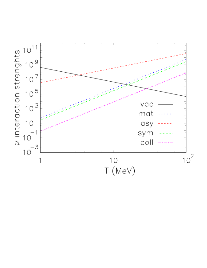
Figure 1: Neutrino collisional and refractive rates (normalized in terms of the Hubble rate) vs. temperature $T$. In particular, we show $\Omega_{\rm vac}$ (solid curve), $\Omega_{\rm matt}$ (long-dotted curve), $\Omega_{\rm asy}\times\Delta_{e}$ (dashed curve), $\Omega_{\rm sym}\times\Sigma_{ee}$ (short-dotted curve), $\Omega_{\rm coll}\times[(g_{s}^{e})^{2}+(g_{s}^{\mu})^{2}]$ (dash-dotted curve). Here we use $\Delta m^{2}_{\rm st}$, $\Delta_{e}=32L/3$ with $L=10^{-4}$ and $\Sigma_{ee}=2$ (see the text for more details on these quantities).

From the Figure above, one realizes that the system remains collisional down to a few MeV, when the collision over Hubble rate drops below 1 on the ordinates. The collisional term also dominates over the vacuum oscillation term at $T\gtrsim 20$ MeV, thus breaking the coherence between different neutrino flavors and preventing significant oscillations. The refractive terms can induce MSW-like resonances between the actives ($a=e,\mu,\tau$) and sterile state when, in the limit of only one mixing angle between the active and the sterile neutrinos, one of the following conditions is satisfied Bell:1998ds

$$\Omega_{\rm vac}\cos 2\theta_{as}-\Omega_{\rm asy}\Delta_{a}+\Omega_{\rm sym}\Sigma_{aa}+\Omega_{\rm mat} = 0\,\ \,\ \textrm{for}\,\ \nu\,\ ,$$

$$\Omega_{\rm vac}\cos 2\theta_{as}+\Omega_{\rm asy}\Delta_{a}+\Omega_{\rm sym}\Sigma_{aa}+\Omega_{\rm mat} = 0\,\ \,\ \textrm{for}\,\ \overline{\nu}\,\ ,$$ (36)

where $a=e,\mu,\tau$ and the definitions of $\Delta_{\mu}$, $\Delta_{\tau}$ and $\Sigma_{\mu\mu}$, $\Sigma_{\tau\tau}$ are respectively of the same form to the ones of $\Delta_{e}$ and $\Sigma_{ee}$ given before. From these equations, we obtain that in absence of lepton asymmetries ($\Delta_{a}=0$) the resonance condition cannot be satisfied neither for the $\nu$’s nor for $\overline{\nu}$’s, given the hypothesis that the sterile state is heavier than the active ones. Instead, when $\Omega_{\rm asy}\Delta_{a}$ is the dominant term, as in the cases we will consider in the following, resonance conditions can occur for $\Delta_{a}>0$ in the $\nu$ sector and for $\Delta_{a}<0$ in the $\overline{\nu}$ one. In particular, in Fig. 1 the resonance occurs around $T\simeq 3$ MeV. We will also show that, as a consequence of the dynamical nature of the asymmetries, $\Delta_{a}$ can rapidly change sign so that both sterile neutrinos and antineutrinos get populated. This phenomenon is thus qualitatively different with respect to the familiar MSW resonant conversion. Resonances can also take place in the active sector at lower temperatures. However, since active neutrino distributions are expected not to depart too much from their equilibrium values, their effect is sub-leading.

IV (3+1) results

In order to calculate the sterile neutrino abundance in the 3+1 scenario, described in Sec. II, we numerically solved the EoMs [Eq. (25)], using a Runge-Kutta method for the equations written in the variable $x=m/T$ and evolved in the range $x\in[10^{-2},1.0]$. We take $10^{5}$ steps in $\log(x)$ in the integration interval. We consider initial neutrino asymmetries $L=L_{e}=L_{\mu}=L_{\tau}<0$. We checked that the results presented in the following do not change considering positive asymmetries. In Fig. 2 we show the evolution of the diagonal component of the density matrix $\rho_{ss}$ for sterile neutrinos in function of the temperature $T$ for different initial lepton asymmetries, namely $L=0$ (solid curve), $L=-10^{-4}$ (dashed curve), $L=-10^{-3}$ (dotted curve), and $L=-10^{-2}$ (dash-dotted curve). As expected from the previous literature, in absence of lepton asymmetries sterile neutrinos are copiously produced at $T\lesssim 30$ MeV until they reach $\rho_{ss}=1$. Instead, including a non-zero initial lepton asymmetry the effect is to suppress the sterile neutrino production as long as $|\Omega_{\rm asy}|\gg|\Omega_{\rm vac}|$. However, these two functions have opposite dependence on the temperature and at some time they will cross. Sterile neutrinos are then produced “resonantly”, albeit with a non-linear, dynamical resonance condition which is itself influenced by the evolution of the system. Increasing the lepton number asymmetry the position of the resonance moves towards lower temperatures, where the resonance is less adiabatic. Indeed, the adiabaticity parameter scales as $\sim T$, as shown in DiBari:2001jk . As a consequence, the sterile production is less efficient increasing $|L|$, as results from Fig. 2. In particular, asymmetries greater than $|L|=10^{-3}$ are required in order to achieve a significant suppression of the sterile neutrino production. Also, the asymmetric term changes sign and thus the resonance can take place in both neutrino and antineutrino sectors, which turn out to be populated almost equally.

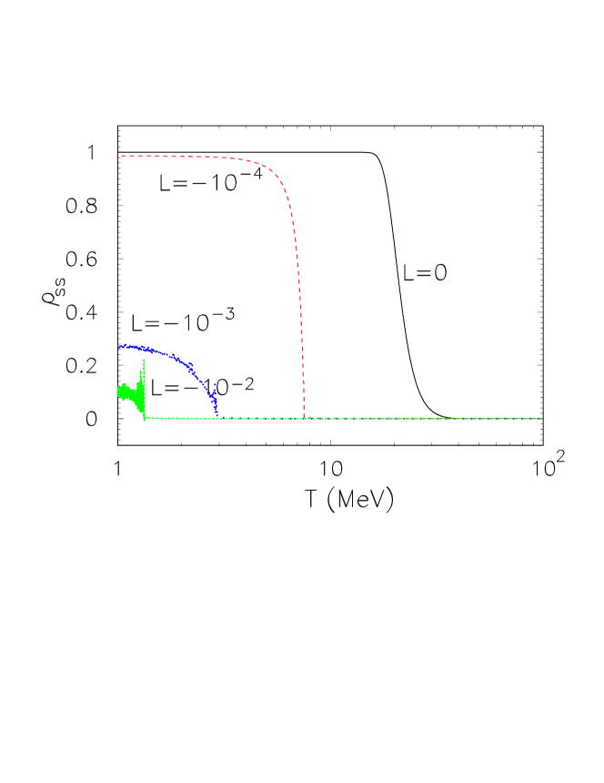
Figure 2: (3+1) scenario. Evolution of the density matrix element $\rho_{ss}$ in function of the temperature $T$. We consider $L=L_{e}=L_{\mu}=L_{\tau}$. The solid curve corresponds to $L=0$, the dashed curve to $L=-10^{-4}$, the dotted curve to $L=-10^{-3}$ and the dash-dotted one to $L=-10^{-2}$.

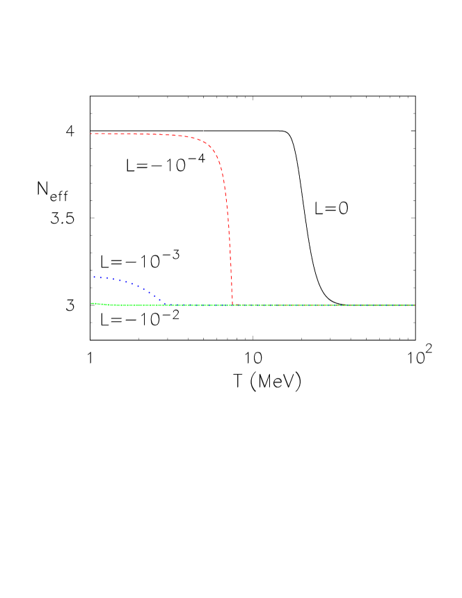
Figure 3: (3+1) scenario. Evolution of the effective number of degrees of freedom $N_{\rm eff}$ for the cases corresponding to Fig. 2

Our result implies that in order to suppress the sterile neutrino production one needs a lepton asymmetry greater at least by an order of magnitude with respect to what found in a previous study on the subject Chu:2006ua . This discrepancy is due to the fact that in their work the authors followed the flavor evolution only for the neutrinos, choosing a negative value of lepton asymmetry kept constant. In this way, they missed resonant effects that would have occurred in the antineutrino sector. Then, the lepton number can only suppress the flavor evolution. Therefore, in their study $L=-10^{-4}$ was enough to block the sterile neutrino production.

Caution should also be taken when interpreting the results shown for $\rho_{ss}$ into an effective increase of the neutrino degrees of freedom in the early universe, usually parameterized via $N_{\rm eff}$. In fact, according to the definition reported in Eq. (19), the latter variable is sensitive to the trace of the neutrino plus antineutrino density matrix. A late conversion of some active state into a sterile one after the neutrinos have undergone collisional decoupling is in fact conserving the overall number of neutrinos (albeit some cosmological consequences, such as those for BBN, may be typically more dramatic, as briefly discussed in Sec. VI). This is shown in Fig. 3, reporting the evolution of $N_{\rm eff}$ for the cases corresponding to Fig. 2. Note that for no or small asymmetry, for the parameters chosen the active-sterile oscillations take place early enough that the depleted active states are rapidly repopulated collisionally. Thus $N_{\rm eff}$ effectively increases to 4. On the other hand, for $|L|=10^{-3}$ the conversion takes place around the decoupling time, and the repopulation is only partial, with a difference between $N_{\rm eff}$ and $\rho_{ss}$ of about 0.1 units (compare Fig. 2 with Fig. 3). Finally, for $|L|=10^{-2}$ only a negligible fraction of the converted active neutrinos are repopulated, despite the fact that about 10% of a “thermal-equivalent” sterile state has been produced. Since of large asymmetries the temperature at which production starts depends on when the equality $\Omega_{\rm vac}=\Omega_{\rm asy}\times\Delta_{e}$ takes place, there is a quite strong dependence of the signatures from the exact values of the active neutrino mass, mixing, and the initial value of $|L|$.

V (2+1) results

In our study we consider initial distributions for active neutrinos close to their equilibrium ones. Therefore, the oscillations among the three active species have a sub-leading role for the evolution of the sterile neutrinos. At this regard, we calculated the flavor conversions in the same cases as before, considering (2+1) sub-sectors with the active mixing associated with $(\Delta m^{2}_{\rm sol},\theta_{12})$ and $(\Delta m^{2}_{\rm atm},\theta_{13})$, respectively. For the cases we compared, we find results very similar to the ones presented in the previous section. Therefore, in order to speed-up the numerical calculations we decide to continue our explorations of sterile neutrino production in different cases, referring to $(2+1)$ scenarios associated with $(\Delta m^{2}_{\rm atm},\theta_{13})$ active sector.

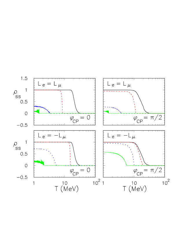
Figure 4: (2+1) scenario. Evolution in function of the temperature $T$ of $\rho_{ss}$ for different initial neutrino asymmetries. Upper panels correspond to $L=L_{e}=L_{\mu}$, lower panels correspond to $L=L_{e}=-L_{\mu}$. The solid curves correspond to $L=0$, the dashed curves to $L=-10^{-4}$, the dotted to $L=-10^{-3}$ and the dash-dotted to $L=-10^{-2}$. Left panels show cases with no CP violation in the sterile neutrino sector, while right panels refers to $\varphi_{\rm CP}=\pi/2$.

V.1 $L_{e}=L_{\mu}$, $\varphi_{CP}=0$

In the following we consider different (2+1) cases with non-zero $\theta_{es}$ and $\theta_{\mu s}$ given by Eq. (6). In the left-upper panel of Fig. 4 we represent the case with $L=L_{e}=L_{\mu}$. The solid curve corresponds to $L=0$, the dashed curve to $L=-10^{-4}$, the dotted curve to $L=-10^{-3}$ and the dash-dotted one to $L=-10^{-2}$. This case is manifestly close to the (3+1) scenario shown in Fig. 2. In order to clarify the dynamics of the sterile neutrino production, in the left panels of Fig. 5 we plot in function of the temperature, the evolution of the neutrino asymmetries $\Delta\rho_{\alpha}=\rho_{\alpha\alpha}-\bar{\rho}_{\alpha\alpha}$ for the $\nu_{e}$ (solid curve), $\nu_{\mu}$ (dotted curve) and $\nu_{s}$ (dashed curve). Since $\Delta\rho_{\alpha}$ typically presents very fast oscillations, for the sake of the clarity we plot its value averaged over ten steps in $T$. In the right panels we show the evolution of the vacuum term $\Omega_{\rm vac}$ (solid curve) and of the $\Omega_{\rm asy}\times\Delta_{e}$ term (dashed curve) for the same cases of the left panels. The crossing between these two curves at non-zero $L$ determines the position of a $e$-$s$ resonance.

Starting with the case $L=0$, we see that $L_{e}=-2L_{\mu}=-2L_{s}\simeq\textrm{few}\times 10^{-5}$ can be dynamically generated at the onset of the flavor conversions (at $T\lesssim 80$ MeV). Since the active asymmetries are opposite, they tend to decrease reaching flavor equilibrium ($L=0$) at $T\simeq 10$ MeV. At $T\lesssim 30$ MeV, when collisional rates slow down enough (see Fig. 1), sterile neutrinos are produced without any hindrance (see Fig. 4).

We pass now to the cases with non-zero initial neutrino asymmetries. In this situation, since $\theta_{es}$ and $\theta_{\mu s}$ are non-vanishing, both the active states can have resonances with the sterile one. Moreover, since for our choice $\theta_{es}\simeq\theta_{\mu s}$, the evolution of $\Delta\rho_{e}$ and $\Delta\rho_{\mu}$ is very similar.

In the case with initial $L=-10^{-4}$ the production of $\nu_{s}$ starts at $T\simeq 10$ MeV (Fig. 4) when an active-sterile resonance occurs. Also in the other two cases with $L=-10^{-3}$ and $L=-10^{-2}$ the position of the resonance coincides with the onset in the rise of $\rho_{ss}$ in Fig. 4. However, as commented before, the lower the resonance temperature, the less adiabatic the resonance. Therefore, the sterile neutrino production is further inhibited.

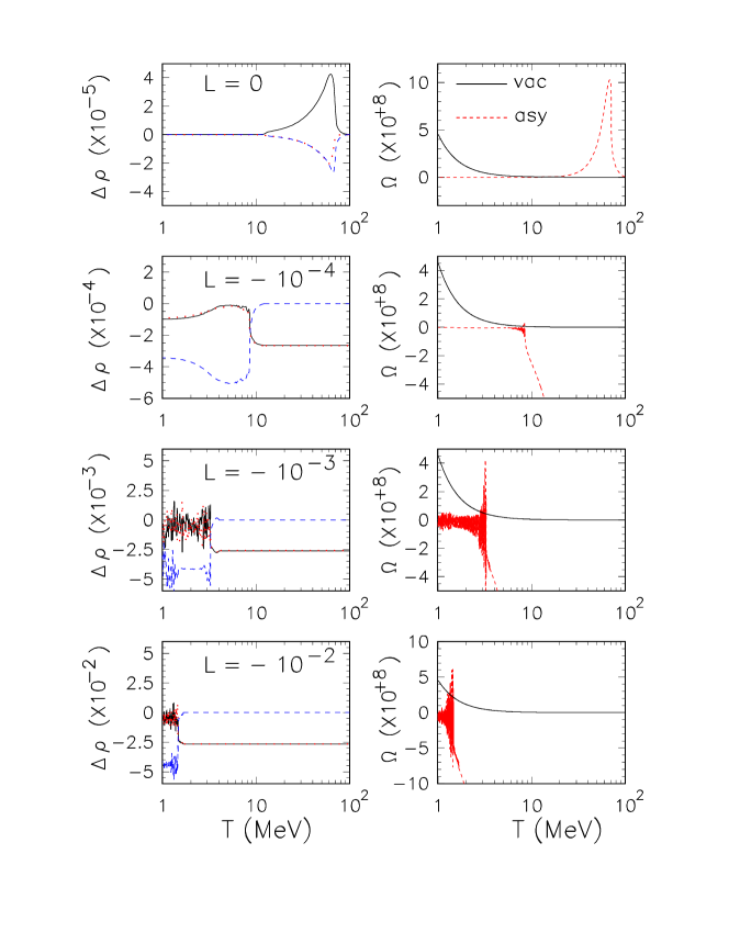
Figure 5: (2+1) case with $L=L_{e}=L_{\mu}$ and $\varphi_{\rm CP}=0$. Left panels: Evolution $\Delta\rho_{\alpha}=\rho_{\alpha\alpha}-\bar{\rho}_{\alpha\alpha}$ for the $\nu_{e}$ (solid curve), $\nu_{\mu}$ (dotted curve) and $\nu_{s}$ (dashed curve) for the different values of initial neutrino asymmetries. Right panels: Evolution of $\Omega_{\rm vac}$ (solid curve) vs $\Omega_{\rm asy}\times\Delta_{e}$ (dashed curve).

V.2 $L_{e}=L_{\mu}$, $\varphi_{CP}=\pi/2$

Fits for laboratory anomalies have been proposed which include CP violation effects in the sterile sector (see e.g. Karagiorgi:2006jf ). Perhaps more importantly, whenever three or more neutrinos mix, CP-violating “Dirac phases” entering oscillations are naturally present in the theory. For both reasons, we find worthwhile to investigate the impact of CP-violation in our framework.

For this purpose, we include an extra phase in the sterile-active mixing matrix [Eq. (4)], formally in the same way the Dirac phase is introduced in $3\times 3$ active neutrino mixing formalism. The inclusion of CP violating effects in the sterile sector could be potentially interesting, since it would generate an asymmetry among sterile neutrinos and antineutrinos. This could be transferred by oscillations into the active sector, having a feedback on the further growth of the sterile neutrino abundance. For definiteness we consider $\varphi_{CP}=\pi/2$. Note also that in the full (3+1) scenario—not to speak of the (3+2) scenarios with 2 sterile states—the number of CP-violating phases grows. Therefore, the present investigation is expected to be conservative in some respect. We first refer to the case with initial equal neutrino asymmetries among active species: $L=L_{e}=L_{\mu}$. The evolution of $\rho_{ss}$ is shown in the right-upper panel of Fig. 4, whose comparison with the CP conserving case shows that the suppression of the sterile neutrino abundance due to $\varphi_{CP}$ is sub-leading. Indeed, from Fig. 6 one sees that the growth of the dynamical neutrino asymmetries $\Delta\rho_{\alpha}$ for different intial $L$, even if it is more irregular than in the case with $\varphi_{\rm CP}=0$ (Fig. 5), it is qualitatively similar. This implies that this effect does not significantly alter the flavor evolution. On the other hand, it is interesting to note that even in absence of an initial neutrino asymmetry the CP-violating mixing can create a “dynamical” asymmetry at relatively late times (down to decoupling temperatures) which is of the order to $10^{-5}$ for the parameters used.

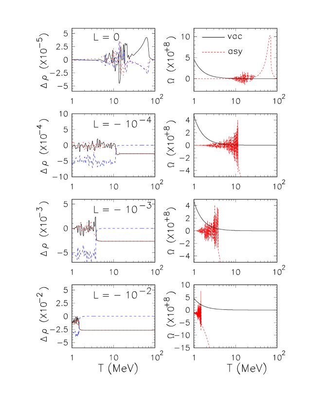
Figure 6: (2+1) case with $L=L_{e}=L_{\mu}$ and $\varphi_{\rm CP}=\pi/2$. Left panels: Evolution $\Delta\rho_{\alpha}=\rho_{\alpha\alpha}-\bar{\rho}_{\alpha\alpha}$ for the $\nu_{e}$ (solid curve), $\nu_{\mu}$ (dotted curve) and $\nu_{s}$ (dashed curve) for the different values of initial neutrino asymmetries. Right panels: Evolution of $\Omega_{\rm vac}$ (solid curve) vs $\Omega_{\rm asy}\times\Delta_{e}$ (dashed curve).

V.3 $L_{e}=-L_{\mu}$, $\varphi_{CP}=0$

We pass now to consider the case in which the initial neutrino asymmetries in the active sector are opposite for $\nu_{e}$ and $\nu_{\mu}$, i.e. $L=L_{e}=-L_{\mu}$. In the absence of CP violation, this case is represented in the bottom-left panel of Fig. 4. For a non-vanishing initial $L$ the sterile neutrino production is enhanced with respect to the previous case with equal asymmetries among the different flavors. Indeed, to achieve a significant suppression of the sterile species one needs an initial $|L|\sim 10^{-2}$, i.e. roughly one order of magnitude larger than in the previous case. This behavior can be clarified looking at the evolution of the dynamical asymmetries $\Delta\rho_{\alpha}$ shown for the different initial $L$ in Fig. 7. We remark that since $\Delta\rho_{e}$ and $\Delta\rho_{\mu}$ have opposite sign, resonances can occur simultaneously in the neutrino and antineutrino channels. When these happen, they tend to produce flavor equilibrium between $\nu_{e}$ and $\nu_{\mu}$. This leads to a vanishing final lepton number. When the neutrino asymmetry is destroyed, the sterile neutrinos can be produced without any hindrance. This explains the enhancement in the final $\rho_{ss}$ found in this case.

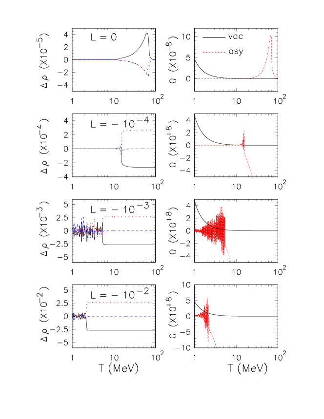
Figure 7: (2+1) case with $L=L_{e}=-L_{\mu}$ and $\varphi_{\rm CP}=0$. Left panels: Evolution $\Delta\rho_{\alpha}=\rho_{\alpha\alpha}-\bar{\rho}_{\alpha\alpha}$ for the $\nu_{e}$ (solid curve), $\nu_{\mu}$ (dotted curve) and $\nu_{s}$ (dashed curve) for the different values of initial neutrino asymmetries. Right panels: Evolution of $\Omega_{\rm vac}$ (solid curve) vs $\Omega_{\rm asy}\times\Delta_{e}$ (dashed curve).

V.4 $L_{e}=-L_{\mu}$, $\varphi_{CP}=\pi/2$

We now consider the case with opposite initial neutrino asymmetries and $\varphi_{\rm CP}=\pi/2$. The evolution of $\rho_{ss}$ in this case is shown in the bottom-right panel of Fig. 4. The production of sterile neutrinos is significantly enhanced with respect to the previous cases. In particular, also for an initial $L=-10^{-2}$, the final abundance of sterile neutrinos is relevant. From Fig. 8 one sees that the flavor equilibrium between the electron and muon species occurs at higher $T$ than in the CP conserving case (Fig. 7). Indeed, CP violating effects tend to create an asymmetry in the sterile sector. This would push the active system earlier to equilibrium in order to conserve the total null neutrino asymmetry. Since $L$ is equilibrated at higher temperature with respect to the CP conserving case, sterile neutrinos are produced more efficiently.

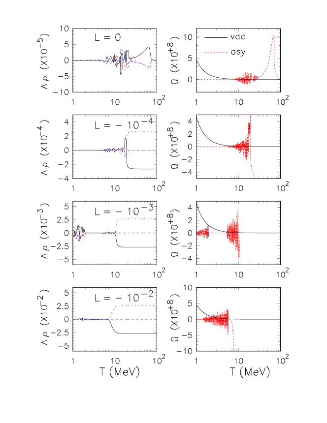
Figure 8: (2+1) case with $L=L_{e}=-L_{\mu}$ and $\varphi_{\rm CP}=\pi/2$. Left panel: Evolution $\Delta\rho_{\alpha}=\rho_{\alpha\alpha}-\bar{\rho}_{\alpha\alpha}$ for the $\nu_{e}$ (solid curve), $\nu_{\mu}$ (dotted curve) and $\nu_{s}$ (dashed curve) for the different values of initial neutrino asymmetries. Right panel: Evolution of $\Omega_{\rm vac}$ (solid curve) vs $\Omega_{\rm asy}\times\Delta_{e}$ (dashed curve).

V.5 $\theta_{\mu s}=0$

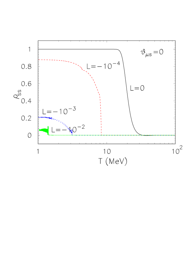
Figure 9: (2+1) case with $\theta_{\mu s}=0$. Evolution of the density matrix element $\rho_{ss}$ in function of the temperature $T$. We consider $L=L_{e}=L_{\mu}$. The solid curve corresponds to $L=0$, the dashed curve to $L=-10^{-4}$, the dotted curve to $L=-10^{-3}$ and the dash-dotted one to $L=-10^{-2}$.

In the recent literature, models in which sterile neutrinos mix only with the (mostly) electron ones have been discussed as well Kopp:2011qd . Hence we also consider a $(2+1)$ case in which the mixing angle $\theta_{\mu s}=0$, while $\theta_{es}$ is given by Eq. (6). The evolution of the sterile neutrino abundance $\rho_{ss}$ in function of $T$ is shown in Fig. 9. For the sake of the brevity, we only consider equal initial neutrino asymmetries $L=L_{e}=L_{\mu}<0$. We represent the cases $L=0$ (solid curve), $L=-10^{-4}$ (dashed curve), $L=-10^{-3}$ (dotted curve), and $L=-10^{-2}$ (dash-dotted curve). From the comparison with the analogous (2+1) case with two active-sterile mixing angles (Fig. 4), we see that the evolution of $\rho_{ss}$ at different $L$ is qualitatively similar. However, for non-zero asymmetries the production of sterile neutrinos is slightly suppressed with respect to the two mixing scenario.

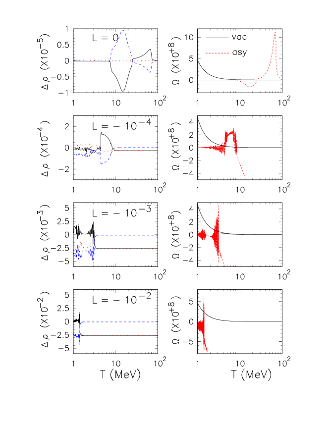
Figure 10: (2+1) case with $\theta_{\mu s}=0$ and $L=L_{e}=L_{\mu}$. Left panels: Evolution $\Delta\rho_{\alpha}=\rho_{\alpha\alpha}-\bar{\rho}_{\alpha\alpha}$ for the $\nu_{e}$ (solid curve), $\nu_{\mu}$ (dotted curve) and $\nu_{s}$ (dashed curve) for the different values of initial neutrino asymmetries. Right panels: Evolution of $\Omega_{\rm vac}$ (solid curve) vs $\Omega_{\rm asy}\times\Delta_{e}$ (dashed curve).

As in the previous cases, in Fig. 10 we plot the evolution of the asymmetries $\Delta\rho_{\alpha}$ for the different values of initial $L$. In the case $L=0$, a value $L_{e}=-L_{s}\simeq\textrm{few}\times 10^{-5}$ can be dynamically generated. Since $\nu_{\mu}$’s are not mixed with the sterile states, their asymmetry remains identically zero. The positive $L_{e}$ can generate a $\nu_{e}$-$\nu_{s}$ resonance in the neutrino sector at $T\simeq 30$ MeV. Then, $L_{e}$ becomes negative reaching a value $L_{e}\simeq-10^{-4}$. After that, the electron and the sterile neutrinos go towards flavor equilibrium (with $L=0$), reaching it at $T\simeq 10$ MeV. In the case with initial $L=-10^{-4}$ the production of $\nu_{s}$ starts at $T\simeq 10$ MeV when a $\nu_{e}$-$\nu_{s}$ resonance occurs. We note that since $\Omega_{\rm asy}\times\Delta_{e}$ is a rapidly oscillating function taking both positive and negative values, resonances affect both neutrino and antineutrino channels. Then, $L_{e}$ reaches a value $\sim 2\times 10^{-3}$, while $L_{\mu}\simeq 0$. A second series of resonances occurs at $T\simeq 4$ MeV, leading $L_{e}$ to zero and $L_{s}\simeq-10^{-4}$. In the last two cases, only one resonance occurs at $T\simeq 3$ MeV for $L=-10^{-3}$, and $T\simeq 0.5$ MeV for $L=-10^{-2}$. Once more the sterile neutrino production is triggered by these resonances.

VI Semi-analytical estimate of the effects on BBN

In order to compute in detail the effects of adding a fourth, sterile neutrino onto BBN, full momentum-dependent calculations are necessary. This is essentially due to the fact that the $\nu_{e}$ and $\overline{\nu}_{e}$ distributions enter the weak rates regulating the neutron-proton equilibrium and, eventually, the amount of surviving neutrons which will mostly end up bound in ⁴He nuclei (plus traces of some other light elements), see Steigman:2007xt ; Iocco:2008va for reviews. We can however provide a crude estimate based on a simple physical argument, which has already been used before in this context (see for example Dolgov:2003sg ). Modifying the neutrino sector alters both the Hubble expansion rate and the overall magnitude of the isospin-changing weak rates $\Gamma_{\rm iso}$, the latter through a change of the neutrino and antineutrino number density parameterized here by $\rho_{ee}$ . Hence the freeze-out temperature $T_{F}$, as defined by the condition

$$\Gamma_{\rm iso}(\rho_{ee},T_{F})=H(N_{\rm eff},T_{F})\,,$$ (37)

is altered with respect to its standard value $T_{F}\simeq 0.8\,$MeV due to a higher-than-standard $N_{\rm eff}$ and a lower-than-standard $\rho_{ee}$. Both effects go in the direction of increasing $T_{F}$ and, as a consequence, anticipate the freeze-out of $n/p$. This ratio is lower then unity due to the fact that neutrons are heavier than protons by $Q=1.293\,$MeV, a non-negligible quantity compared to the energies involved when $T$ drops to the MeV scale. Since the ⁴He mass abundance $Y_{p}$ is proportional to the $n/p$ ratio at freeze-out

$$Y_{p}\propto\left(\frac{n}{p}\right)_{T_{F}}\propto e^{-Q/T_{F}}\,,$$ (38)

we obtain the estimate

$$\frac{\delta Y_{p}}{Y_{p}}=\frac{Q}{T_{F}}\frac{\delta T_{F}}{T_{F}}\simeq 1.6\frac{\delta T_{F}}{T_{F}}\,,$$ (39)

which confirms that we expect an increase in the produced yield. A simple estimate Dolgov:2003sg for the Hubble parameter $H\propto\sqrt{22/7+N_{\rm eff}}\,T^{2}$ and the weak rates $\Gamma_{\rm iso}\propto(1+\rho_{ee})\,T^{5}$ predicts

$$T_{F}\propto\left(\frac{\sqrt{22/7+N_{\rm eff}}}{1+\rho_{ee}}\right)^{1/3}\,,$$ (40)

which immediately illustrates why $Y_{p}$ is comparatively much more sensitive to alteration of the weak rates than to the expansion rate via $N_{\rm eff}$. A perturbative expansion around the fiducial values $N_{\rm eff}=3$ and $\rho_{ee}=1$ yields

$$\frac{\delta T_{F}}{T_{F}}=0.027\,\delta N_{\rm eff}-0.17\,\delta\rho_{ee}\Longrightarrow\frac{\delta Y_{p}}{Y_{p}}=0.044\,\delta N_{\rm eff}-0.27\,\delta\rho_{ee}\,.$$ (41)

For specific cases suggested by our previous analysis, e.g. for the (3+1) results of Sec. IV, one finds for example that for $L=0$, $\delta\rho_{ee}\simeq 0$ while $\delta N_{\rm eff}\simeq 1$, hence one deduces a variation in the Helium content of $4.4\%$, which is a large number and barely allowed (see e.g. Mangano:2011ar ). For the largest asymmetries we considered, $|L|=10^{-2}$, the variation in $N_{\rm eff}$ is negligible while $\delta\rho_{ee}\simeq-0.05$, implying again a few percent effects on $Y_{p}$. For intermediate values like $|L|=10^{-3}$, one expects again effects above the 1% level, this time with both terms contributing. Note that such effects are larger than theoretical uncertainties and comparable to observational ones, hence they do imply that sterile neutrinos cannot be “easily masked” to BBN: they do have an impact that must be accounted for in any realistic analysis combining cosmological observables. The above estimates should be considered only as illustrative, lacking a proper account of momentum-dependent effects in weak rates. We plan to provide a more reliable estimate of their impact in a future work.

VII Conclusions

Light sub-eV sterile neutrinos, suggested to solve different anomalies in short-baseline, reactor and solar experiments Akhmedov:2010vy ; Kopp:2011qd ; Giunti:2011gz ; Giunti:2011hn , could play an interesting cosmological role providing the amount of extra-radiation indicated by different cosmological observations Hamann:2010bk . However, for the scenarios proposed to fit the different laboratory data, sterile neutrinos would be produced too copiously in the early universe by the mixing with the active species. This would create a tension between the laboratory hints and the cosmological observations Hamann:2011ge . A possibility to reconcile sterile neutrinos with cosmology is the introduction of a primordial neutrino asymmetry Foot:1995bm , that is expected to suppress the sterile-active mixing when its strength dominates over the other interaction terms. In this context, we calculated the sterile neutrino abundance in the early universe in (3+1) and (2+1) schemes solving the neutrino kinetic equations for different initial asymmetries. Considering approximately equilibrium distributions for the active neutrino species, the flavor dynamics of active neutrinos plays a sub-leading role in determining the final abundance of the sterile species. Therefore, (2+1) schemes are a good proxy for the complete (3+1) situation. Starting with initial neutrino asymmetries equal for the two active species, $|L|\simeq 10^{-3}$ would be required to have a significant suppression of the neutrino abundance. Otherwise, sterile neutrinos would be produced by resonances between the vacuum term and the evolving (oscillating) active $\nu-\overline{\nu}$ asymmetry potential. Opposite initial neutrino asymmetries (hence a globally vanishing lepton number) would cuase an enhancement in the sterile neutrino production compared to the above case, implying $|L|\gtrsim 10^{-2}$ to substantially inhibit their creation. Moreover, in this last case the presence of CP violating effects would further increase the sterile neutrino abundance, requiring an even larger initial asymmetry to prevent their growth. Both the assumptions of non-dynamical asymmetries and, to a minor extent, of mixing with a single active neutrino tend to underestimate the value of $|L|$ needed for inhibiting the sterile $\nu$ production.

Coming to phenomenological consequences, this suggests that some proposed ways to reconcile “hints for a large $N_{\rm eff}$” from CMB with more stringent requirements from BBN, via the introduction of large chemical potentials (see e.g. Hamann:2011ge ) are dynamically hard—if not impossible—to achieve. Whenever CMB feels a large $N_{\rm eff}$ due to sterile neutrinos of the kind suggested by laboratory anomalies, BBN should feel the same. However, the opposite situation is not necessarily true. Even more interestingly, we found that whenever a significant suppression of the sterile neutrino production takes place thanks to initial asymmetries, the active neutrinos have partially or mostly decoupled. This implies that the (small) fraction of them which oscillates into sterile states is not repopulated. Hence, one expects different possible regimes: For too small asymmetries, $|L|\ll 10^{-3}$, the sterile neutrinos are fully populated and their “parent” active neutrino spectra are repopulated in the thermal plasma. This implies $N_{\rm eff}\simeq 4$ (for (3+1) scenarios considered here) and a tension with cosmological mass bounds, which counteracts the modest fit improvements due to a larger $N_{\rm eff}$. Increasing the asymmetry ($|L|\gtrsim 10^{-3}$) the effect on $N_{\rm eff}$ becomes less and less prominent, and completely negligible when $|L|\gtrsim 10^{-2}$. However, the lack of repopulation of electron neutrinos would in general produce distorted distributions, which can anticipate the $n/p$ freeze-out and hence increase the ⁴He yield, to which BBN is much more sensitive than CMB. Finally, for a too large $|L|$, no production/depletion takes place, but these asymmetries in the active flavors would then become an interesting cosmological observable to be associated with sterile neutrinos.

To go beyond semi-analytical estimates, especially to detail the intermediate regime, one has to relax the average momentum approximation used in this exploratory study. Due to the momentum-dependence of the resonant conversions between active and sterile neutrinos, a detailed treatment solving the full momentum-dependent equations is necessary to derive quantitative phenomenological predictions. We plan to perform this exploration in a forthcoming article. Also note that our study suggests that the dynamics of sterile neutrinos in the early universe is quite dependent on the details of the scenario considered. Pinning down the parameters favored by interpretations of the laboratory data in terms of sterile states is crucial in order to treat in the most accurate way only scenarios which are phenomenologically attractive. Large scans of parameter space obtained in too crude approximations might miss essential aspects of the problem, which is intrinsically non-linear.

References

References

- (1) K. N. Abazajian, et al., “Light Sterile Neutrinos: A White Paper,” arXiv:1204.5379 [hep-ph].
- (2) A. Aguilar-Arevalo et al. [LSND Collaboration], “Evidence for neutrino oscillations from the observation of anti-neutrino(electron) appearance in a anti-neutrino(muon) beam,” Phys. Rev. D 64, 112007 (2001) [hep-ex/0104049].
- (3) A. A. Aguilar-Arevalo et al. [The MiniBooNE Collaboration], “Event Excess in the MiniBooNE Search for Oscillations,” Phys. Rev. Lett. 105, 181801 (2010) [arXiv:1007.1150 [hep-ex]].
- (4) G. Mention, M. Fechner, T. Lasserre, T. A. Mueller, D. Lhuillier, M. Cribier and A. Letourneau, “The Reactor Antineutrino Anomaly,” Phys. Rev. D 83, 073006 (2011) [arXiv:1101.2755 [hep-ex]].
- (5) M. A. Acero, C. Giunti and M. Laveder, “Limits on nu(e) and anti-nu(e) disappearance from Gallium and reactor experiments,” Phys. Rev. D 78, 073009 (2008) [arXiv:0711.4222 [hep-ph]].
- (6) E. Akhmedov and T. Schwetz, “MiniBooNE and LSND data: Non-standard neutrino interactions in a (3+1) scheme versus (3+2) oscillations,” JHEP 1010, 115 (2010) [arXiv:1007.4171 [hep-ph]].
- (7) J. Kopp, M. Maltoni and T. Schwetz, “Are there sterile neutrinos at the eV scale?,” Phys. Rev. Lett. 107, 091801 (2011) [arXiv:1103.4570 [hep-ph]].
- (8) C. Giunti and M. Laveder, “3+1 and 3+2 Sterile Neutrino Fits,” Phys. Rev. D 84, 073008 (2011) [arXiv:1107.1452 [hep-ph]].
- (9) C. Giunti and M. Laveder, “Status of 3+1 Neutrino Mixing,” Phys. Rev. D 84, 093006 (2011) [arXiv:1109.4033 [hep-ph]].
- (10) A. Donini, P. Hernandez, J. Lopez-Pavon, M. Maltoni and T. Schwetz, “The minimal 3+2 neutrino model versus oscillation anomalies,” JHEP 1207, 161 (2012) [arXiv:1205.5230 [hep-ph]].
- (11) A. D. Dolgov, “Neutrinos in the Early Universe,” Sov. J. Nucl. Phys. 33, 700 (1981) [Yad. Fiz. 33, 1309 (1981)].
- (12) R. Barbieri and A. Dolgov, “Bounds on Sterile-neutrinos from Nucleosynthesis,” Phys. Lett. B 237, 440 (1990).
- (13) R. Barbieri and A. Dolgov, “Neutrino oscillations in the early universe,” Nucl. Phys. B 349, 743 (1991).
- (14) K. Enqvist, K. Kainulainen and J. Maalampi, “Refraction And Oscillations Of Neutrinos In The Early Universe,” Nucl. Phys. B 349, 754 (1991).
- (15) G. Mangano, G. Miele, S. Pastor, T. Pinto, O. Pisanti and P. D. Serpico, “Relic neutrino decoupling including flavor oscillations,” Nucl. Phys. B 729, 221 (2005) [hep-ph/0506164].
- (16) G. Mangano, G. Miele, S. Pastor, T. Pinto, O. Pisanti and P. D. Serpico, “Effects of non-standard neutrino-electron interactions on relic neutrino decoupling,” Nucl. Phys. B 756, 100 (2006) [hep-ph/0607267].
- (17) J. Hamann, S. Hannestad, G. G. Raffelt, I. Tamborra and Y. Y. Y. Wong, “Cosmology seeking friendship with sterile neutrinos,” Phys. Rev. Lett. 105, 181301 (2010) [arXiv:1006.5276 [hep-ph]].
- (18) M. C. Gonzalez-Garcia, M. Maltoni and J. Salvado, “Robust Cosmological Bounds on Neutrinos and their Combination with Oscillation Results,” JHEP 1008, 117 (2010) [arXiv:1006.3795 [hep-ph]].
- (19) E. Komatsu et al. [WMAP Collaboration], “Seven-Year Wilkinson Microwave Anisotropy Probe (WMAP) Observations: Cosmological Interpretation,” Astrophys. J. Suppl. 192, 18 (2011) [arXiv:1001.4538 [astro-ph.CO]].
- (20) C. L. Reichardt, P. A. R. Ade, J. J. Bock, J. R. Bond, J. A. Brevik, C. R. Contaldi, M. D. Daub and J. T. Dempsey et al., “High resolution CMB power spectrum from the complete ACBAR data set,” Astrophys. J. 694, 1200 (2009) [arXiv:0801.1491 [astro-ph]].
- (21) S. Das, T. A. Marriage, P. A. R. Ade, P. Aguirre, M. Amir, J. W. Appel, L. F. Barrientos and E. S. Battistelli et al., “The Atacama Cosmology Telescope: A Measurement of the Cosmic Microwave Background Power Spectrum at 148 and 218 GHz from the 2008 Southern Survey,” Astrophys. J. 729, 62 (2011) [arXiv:1009.0847 [astro-ph.CO]].
- (22) Z. Hou, R. Keisler, L. Knox, M. Millea and C. Reichardt, “How Additional Massless Neutrinos Affect the Cosmic Microwave Background Damping Tail,” arXiv:1104.2333 [astro-ph.CO].
- (23) G. Mangano and P. D. Serpico, “A robust upper limit on from BBN, circa 2011,” Phys. Lett. B 701, 296 (2011) [arXiv:1103.1261 [astro-ph.CO]].
- (24) J. Hamann, S. Hannestad, G. G. Raffelt and Y. Y. Y. Wong, “Sterile neutrinos with eV masses in cosmology: How disfavoured exactly?,” JCAP 1109, 034 (2011) [arXiv:1108.4136 [astro-ph.CO]].
- (25) J. Lesgourgues and S. Pastor, “Massive neutrinos and cosmology,” Phys. Rept. 429, 307 (2006) [astro-ph/0603494].
- (26) Y. Y. Y. Wong, “Neutrino mass in cosmology: status and prospects,” Ann. Rev. Nucl. Part. Sci. 61, 69 (2011) [arXiv:1111.1436 [astro-ph.CO]].
- (27) E. Giusarma, M. Archidiacono, R. de Putter, A. Melchiorri and O. Mena, “Sterile neutrino models and nonminimal cosmologies,” Phys. Rev. D 85, 083522 (2012) [arXiv:1112.4661 [astro-ph.CO]].
- (28) S. Dodelson, A. Melchiorri and A. Slosar, “Is cosmology compatible with sterile neutrinos?,” Phys. Rev. Lett. 97, 041301 (2006) [astro-ph/0511500].
- (29) S. Joudaki, K. N. Abazajian and M. Kaplinghat, “Are Light Sterile Neutrinos Preferred or Disfavored by Cosmology?,” arXiv:1208.4354 [astro-ph.CO].
- (30) B. H. J. McKellar and M. J. Thomson, “Oscillating doublet neutrinos in the early universe,” Phys. Rev. D 49, 2710 (1994).
- (31) G. Sigl and G. Raffelt, “General kinetic description of relativistic mixed neutrinos,” Nucl. Phys. B 406, 423 (1993).
- (32) K. Enqvist, K. Kainulainen and J. Maalampi, “Resonant neutrino transitions and nucleosynthesis,” Phys. Lett. B 249, 531 (1990).
- (33) K. Enqvist, K. Kainulainen and M. J. Thomson, “Stringent cosmological bounds on inert neutrino mixing,” Nucl. Phys. B 373, 498 (1992).
- (34) K. Enqvist, K. Kainulainen and J. Maalampi, “Neutrino Asymmetry And Oscillations In The Early Universe,” Phys. Lett. B 244, 186 (1990).
- (35) P. Di Bari, P. Lipari and M. Lusignoli, “The muon-neutrino s neutrino interpretation of the atmospheric neutrino data and cosmological constraints,” Int. J. Mod. Phys. A 15, 2289 (2000) [hep-ph/9907548].
- (36) P. Di Bari and R. Foot, “On the sign of the neutrino asymmetry induced by active sterile neutrino oscillations in the early universe,” Phys. Rev. D 61, 105012 (2000) [hep-ph/9912215].
- (37) P. Di Bari and R. Foot, “Active sterile neutrino oscillations and BBN + CMBR constraints,” Phys. Rev. D 63, 043008 (2001) [hep-ph/0008258].
- (38) P. Di Bari, “Update on neutrino mixing in the early universe,” Phys. Rev. D 65, 043509 (2002) [Addendum-ibid. D 67, 127301 (2003)] [hep-ph/0108182].
- (39) A. D. Dolgov, S. H. Hansen, S. Pastor and D. V. Semikoz, “Neutrino oscillations in the early universe: How large lepton asymmetry can be generated?,” Astropart. Phys. 14, 79 (2000) [hep-ph/9910444].
- (40) P. Di Bari, R. Foot, R. R. Volkas and Y. Y. Y. Wong, “Comment on ‘Neutrino oscillations in the early universe: How can large lepton asymmetry be generated?’,” Astropart. Phys. 15, 391 (2001) [hep-ph/0008245].
- (41) R. Foot and R. R. Volkas, “Reconciling sterile neutrinos with big bang nucleosynthesis,” Phys. Rev. Lett. 75, 4350 (1995) [hep-ph/9508275].
- (42) R. Foot, M. J. Thomson and R. R. Volkas, “Large neutrino asymmetries from neutrino oscillations,” Phys. Rev. D 53, R5349 (1996) [hep-ph/9509327].
- (43) N. F. Bell, R. R. Volkas and Y. Y. Y. Wong, “Relic neutrino asymmetry evolution from first principles,” Phys. Rev. D 59, 113001 (1999) [hep-ph/9809363].
- (44) D. P. Kirilova and M. V. Chizhov, “Cosmological nucleosynthesis and active sterile neutrino oscillations with small mass differences: The Nonresonant case,” Phys. Rev. D 58, 073004 (1998) [hep-ph/9707282].
- (45) D. P. Kirilova and M. V. Chizhov, “Cosmological nucleosynthesis and active sterile neutrino oscillations with small mass differences: The Resonant case,” Nucl. Phys. B 591, 457 (2000) [hep-ph/9909408].
- (46) K. Abazajian, N. F. Bell, G. M. Fuller and Y. Y. Y. Wong, “Cosmological lepton asymmetry, primordial nucleosynthesis, and sterile neutrinos,” Phys. Rev. D 72, 063004 (2005) [astro-ph/0410175].
- (47) C. T. Kishimoto, G. M. Fuller and C. J. Smith, “Coherent Active-Sterile Neutrino Flavor Transformation in the Early Universe,” Phys. Rev. Lett. 97, 141301 (2006) [astro-ph/0607403].
- (48) A. D. Dolgov and F. L. Villante, “BBN bounds on active sterile neutrino mixing,” Nucl. Phys. B 679, 261 (2004) [hep-ph/0308083].
- (49) M. Cirelli, G. Marandella, A. Strumia and F. Vissani, “Probing oscillations into sterile neutrinos with cosmology, astrophysics and experiments,” Nucl. Phys. B 708, 215 (2005) [hep-ph/0403158].
- (50) Y. -Z. Chu and M. Cirelli, “Sterile neutrinos, lepton asymmetries, primordial elements: How much of each?,” Phys. Rev. D 74, 085015 (2006) [astro-ph/0608206].
- (51) K. N. Abazajian and P. Agrawal, “Chaos, Determinacy and Fractals in Active-Sterile Neutrino Oscillations in the Early Universe,” JCAP 0810, 006 (2008) [arXiv:0807.0456 [hep-ph]].
- (52) A. Melchiorri, O. Mena, S. Palomares-Ruiz, S. Pascoli, A. Slosar and M. Sorel, “Sterile Neutrinos in Light of Recent Cosmological and Oscillation Data: A Multi-Flavor Scheme Approach,” JCAP 0901, 036 (2009) [arXiv:0810.5133 [hep-ph]].
- (53) S. Hannestad, I. Tamborra and T. Tram, “Thermalisation of light sterile neutrinos in the early universe,” JCAP 1207, 025 (2012) [arXiv:1204.5861 [astro-ph.CO]].
- (54) A. D. Dolgov, S. H. Hansen, S. Pastor, S. T. Petcov, G. G. Raffelt and D. V. Semikoz, “Cosmological bounds on neutrino degeneracy improved by flavor oscillations,” Nucl. Phys. B 632, 363 (2002) [hep-ph/0201287].
- (55) P. D. Serpico and G. G. Raffelt, “Lepton asymmetry and primordial nucleosynthesis in the era of precision cosmology,” Phys. Rev. D 71, 127301 (2005) [astro-ph/0506162].
- (56) S. Pastor, T. Pinto and G. G. Raffelt, “Relic density of neutrinos with primordial asymmetries,” Phys. Rev. Lett. 102, 241302 (2009) [arXiv:0808.3137 [astro-ph]].
- (57) G. Mangano, G. Miele, S. Pastor, O. Pisanti and S. Sarikas, “Constraining the cosmic radiation density due to lepton number with Big Bang Nucleosynthesis,” JCAP 1103, 035 (2011) [arXiv:1011.0916 [astro-ph.CO]].
- (58) E. Di Valentino, M. Lattanzi, G. Mangano, A. Melchiorri and P. Serpico, “Future constraints on neutrino isocurvature perturbations in the curvaton scenario,” Phys. Rev. D 85, 043511 (2012) [arXiv:1111.3810 [astro-ph.CO]].
- (59) G. Mangano, G. Miele, S. Pastor, O. Pisanti and S. Sarikas, “Updated BBN bounds on the cosmological lepton asymmetry for non-zero ,” Phys. Lett. B 708, 1 (2012) [arXiv:1110.4335 [hep-ph]].
- (60) E. Castorina, U. Franca, M. Lattanzi, J. Lesgourgues, G. Mangano, A. Melchiorri and S. Pastor, “Cosmological lepton asymmetry with a nonzero mixing angle ,” arXiv:1204.2510 [astro-ph.CO].
- (61) J. A. Harvey and E. W. Kolb, “Grand Unified Theories And The Lepton Number Of The Universe,” Phys. Rev. D 24, 2090 (1981).
- (62) A. Casas, W. Y. Cheng and G. Gelmini, “Generation of large lepton asymmetries,” Nucl. Phys. B 538, 297 (1999) [hep-ph/9709289].
- (63) A. D. Dolgov, “Neutrinos in cosmology,” Phys. Rept. 370, 333 (2002) [hep-ph/0202122].
- (64) L. Wolfenstein, “Neutrino Oscillations In Matter,” Phys. Rev. D 17, 2369 (1978); S. P. Mikheev and A. Yu. Smirnov, “Resonance Enhancement Of Oscillations In Matter And Solar Neutrino Spectroscopy,” Yad. Fiz. 42, 1441 (1985) [Sov. J. Nucl. Phys. 42, 913 (1985)].
- (65) J. Gava and C. Volpe, “CP violation effects on the neutrino degeneracy parameters in the Early Universe,” Nucl. Phys. B 837, 50 (2010) [arXiv:1002.0981 [hep-ph]].
- (66) C. Giunti and C. W. Kim, “Fundamentals of Neutrino Physics and Astrophysics”, Oxford University Press 2007.
- (67) M. Maltoni, T. Schwetz and J. W. F. Valle, “Status of four neutrino mass schemes: A Global and unified approach to current neutrino oscillation data,” Phys. Rev. D 65, 093004 (2002) [hep-ph/0112103].
- (68) K. Nakamura et al. [Particle Data Group Collaboration], “Review of particle physics,” J. Phys. G G 37 (2010) 075021.
- (69) G. L. Fogli, E. Lisi, A. Marrone, D. Montanino, A. Palazzo and A. M. Rotunno, “Global analysis of neutrino masses, mixings and phases: entering the era of leptonic CP violation searches,” Phys. Rev. D 86, 013012 (2012) [arXiv:1205.5254 [hep-ph]].
- (70) D. V. Forero, M. Tortola and J. W. F. Valle, “Global status of neutrino oscillation parameters after recent reactor measurements,” arXiv:1205.4018 [hep-ph].
- (71) K. Abe et al. [T2K Collaboration], “Indication of Electron Neutrino Appearance from an Accelerator-produced Off-axis Muon Neutrino Beam,” Phys. Rev. Lett. 107, 041801 (2011) [arXiv:1106.2822 [hep-ex]].
- (72) P. Adamson et al. [MINOS Collaboration], “Improved search for muon-neutrino to electron-neutrino oscillations in MINOS,” Phys. Rev. Lett. 107, 181802 (2011) [arXiv:1108.0015 [hep-ex]].
- (73) Y. Abe et al. [DOUBLE-CHOOZ Collaboration], “Indication for the disappearance of reactor electron antineutrinos in the Double Chooz experiment,” Phys. Rev. Lett. 108, 131801 (2012) [arXiv:1112.6353 [hep-ex]].
- (74) G. L. Fogli, E. Lisi, A. Marrone, A. Palazzo and A. M. Rotunno, “Hints of theta(13) 0 from global neutrino data analysis,” Phys. Rev. Lett. 101, 141801 (2008) [arXiv:0806.2649 [hep-ph]].
- (75) G. L. Fogli, E. Lisi, A. Marrone, A. Palazzo and A. M. Rotunno, “Evidence of from global neutrino data analysis,” Phys. Rev. D 84, 053007 (2011) [arXiv:1106.6028 [hep-ph]].
- (76) F. P. An et al. [DAYA-BAY Collaboration], “Observation of electron-antineutrino disappearance at Daya Bay,” Phys. Rev. Lett. 108, 171803 (2012) [arXiv:1203.1669 [hep-ex]].
- (77) J. K. Ahn et al. [RENO Collaboration], “Observation of Reactor Electron Antineutrino Disappearance in the RENO Experiment,” Phys. Rev. Lett. 108, 191802 (2012) [arXiv:1204.0626 [hep-ex]].
- (78) G. L. Fogli, E. Lisi, A. Marrone and A. Palazzo, “Global analysis of three-flavor neutrino masses and mixings,” Prog. Part. Nucl. Phys. 57, 742 (2006) [hep-ph/0506083].
- (79) P. Di Bari and R. Foot, “Active sterile neutrino oscillations in the early universe: Asymmetry generation at low —delta m**2— and the Landau-Zener approximation,” Phys. Rev. D 65, 045003 (2002) [hep-ph/0103192].
- (80) G. Karagiorgi, A. Aguilar-Arevalo, J. M. Conrad, M. H. Shaevitz, K. Whisnant, M. Sorel and V. Barger, “Leptonic CP violation studies at MiniBooNE in the (3+2) sterile neutrino oscillation hypothesis,” Phys. Rev. D 75, 013011 (2007) [Erratum-ibid. D 80, 099902 (2009)] [hep-ph/0609177].
- (81) G. Steigman, “Primordial Nucleosynthesis in the Precision Cosmology Era,” Ann. Rev. Nucl. Part. Sci. 57, 463 (2007) [arXiv:0712.1100 [astro-ph]].
- (82) F. Iocco, G. Mangano, G. Miele, O. Pisanti and P. D. Serpico, “Primordial Nucleosynthesis: from precision cosmology to fundamental physics,” Phys. Rept. 472, 1 (2009) [arXiv:0809.0631 [astro-ph]].