Gaussian quantum computation with oracle-decision problems

Abstract

We study a simple-harmonic-oscillator quantum computer solving oracle decision problems. We show that such computers can perform better by using nonorthogonal Gaussian wave functions rather than orthogonal top-hat wave functions as input to the information encoding process. Using the Deutsch -Jozsa problem as an example, we demonstrate that Gaussian modulation with optimized width parameter results in a lower error rate than for the top-hat encoding. We conclude that Gaussian modulation can allow for an improved trade-off between encoding, processing and measurement of the information.

I Introduction

The process of computation involves taking an input and converting it into an output through the application of an algorithm CLRS01 ; Si97 . There are two versions of classical computation: digital and analogue. Digital computers use finite-length bit strings as the input and output of the computer. Analogue computers typically use the electrical quantities of inductance and charge as analogues of mass and displacement so that continuously varying voltages may output, for example, the simulated trajectory of a spacecraft Ja74 .

Quantum computation also has two versions of information processing referred to as discrete-variable NC00 and continuous-variable BP03 quantum computation. In the discrete-variable version, algorithms employ a finite numbers of qubits NC00 or qudits GKP01 analogously to bits in the classical digital case. Continuous-variable quantum computation uses continuously-parameterized quantum systems to process discrete information.

Comparing the performance of a well-known problem and its algorithm in both discrete and continuous settings provides useful insight into how the different versions of quantum computation differ in their performance. The historically important Deutsch–Jozsa problem De85 ; DJ92 has been used to show the different algorithm performance that can be achieved in the two settings. In the discrete variable setting, the Deutsch–Jozsa problem can solved exactly with a single query of a quantum oracle DJ92 . In the continuous variable setting, quantum algorithms employing orthogonal wave functions as the computational basis necessarily have single-query success probability less than one AHS09 .

Continuous-variable studies are often based on quantum optics because of the wide variety of tools that have been developed to process and measure optical field modes BP03 ; FSB98 ; GG02 ; AFK08 ; AYA07 ; Br98 ; EP02 ; BSBN02 ; BS02 . Continuous-variable quantum algorithms have been studied that use a single mode AHS09 and multiple modes CHMS10 . In continuous-variable quantum information procedures, the input state is typically a Gaussian wave function over the canonical position representation with the physical system being a harmonic oscillator (equivalently a single-mode optical field Le97 ). However the unbounded extent of these wave functions does not naturally fit with the finite length of the information strings being processed.

To deal with the problem of finite-length information strings, the single-mode algorithm defined in AHS09 has input states represented by orthogonal wave functions. Information is represented by finite-length bit strings $z\in\{0,1\}^{N}$ with $N$ the number of bits. These strings are encoded into a region of the momentum domain $p$ extending from $-P$ to $P$. A regular lattice of $N$ discrete values of $p$ are embedded in this domain such that the $i^{\rm{th}}$ bit of $z$, is assigned to $p$ as follows: $p_{z_{i}}:=(1+2i-N\pm 1)P/N$. The lattice is thus $\{p_{z_{i}}\}$ with spacing $2P/N$.

An orthogonal basis of top-hat functions is formed from the $p_{z_{i}}$, and the encoded momentum wave function is expressed as $\frac{1}{\sqrt{2P}}\sum_{i=0}^{N-1}(-1)^{z_{i}}\left|p_{z_{i}}\right\rangle$. The kets $\left|p_{z_{i}}\right\rangle$ are phase-modulated by their corresponding bit values, and with this phase modulation, each of the possible $2^{N}$ strings is uniquely represented. Note that the constant wave function is the top-hat function extending from $-P$ to $P$.

There is a translational invariance between computational basis states because each of the top-hat basis functions occupies an identically-sized region of momentum space and because the string $z^{\prime}$ is obtained from the string $z$ by the translation $z^{\prime}=z\oplus(z\oplus z^{\prime})$. We can regard this finite basis as an infinite basis modulated by a top-hat function extending from $-P$ to $P$, which has the effect of truncating the allowed strings from an infinite domain to being from $0$ to $N-1$.

In this paper, we extend this approach by shaping the overall top-hat function with a Gaussian having width set by its standard deviation $\sigma$. The Gaussian is truncated for $|p|>P$, which has the effect that the computational basis states, although still orthogonal, are no longer translations of each other but are more complicated Gaussian-modulated basis states. At first glance, this latter feature would appear to provide a disadvantage, but using the mathematical properties of the error function, we prove that the single-query success probability for the Gaussian case $\Pr_{\checkmark}^{\sharp}>\Pr_{\checkmark}^{\bot}$ is greater than the single-query success probability for the orthogonal case.

This result is enabled by the extra degree of freedom manifest in the spread of the Gaussian wave function. Tuning the available parameters of encoding width, the spread of the Gaussian wave function and the width of the measurement window results in a more efficiently encoded momentum wave function leading to the improved single-query success probability. Note that the use of the top-hat basis to encode information into a single harmonic oscillator is different than the approach used in GKP01 , where information is encoded into a collection of harmonic oscillators.

Our paper is organized as follows. In Sec. II, we define oracle-decision problems and present the Deutsch–Jozsa  DJ92 ; De85 ; CEMM98 in this context. We give an overview of the single-mode algorithm employing orthogonal states AHS09 that solves the Deutsch–Jozsa problem. We give a brief introduction into the coherent states of the harmonic oscillator and define the single-mode algorithm in these terms. In Sec. III, we prove that the single-query success probability claimed for the Gaussian model with truncated momentum is better than that achieved using orthogonal states AHS09 . We conclude in Sec. IV.

II Background

An important aspect of quantum information processing is the ability to solve oracle decision problems with increased efficiency compared to classical information processing. In the case of oracle decision problems, efficiency is measured in terms of the number of oracle queries required to solve the problem. Comparing the single-query success probability of an algorithm in both the discrete and continuous quantum settings provides useful insights into the advantages of one setting over the other. The Deutsch–Jozsa oracle-decision problem has been studied in both the discrete and continuous-variable quantum settings  DJ92 ; BP03 ; AHS09 ; AHS11 . Here we explore a single-mode continuous-variable quantum algorithm where the input state is a Gaussian wave function.

II.1 Oracle Decision Problems and the Deutsch–Jozsa Problem

The challenge of an oracle decision problem is to identify which of two mutually disjoint sets contains a unique $N$-bit string by making the fewest possible queries to an oracle. The oracle decision problem is typically couched in terms of a function $f$ that maps $N=2^{n}$-bit strings to a single bit

$$f:\{0,1\}^{n}\mapsto\{0,1\}.$$ (1)

Any Boolean function on $n$ bits can also be represented by a string of $N=2^{n}$ bits, in which the $i^{\rm{th}}$ bit $z_{i}$ is the value of the function on the $i^{\rm{th}}$ bit string, taken in lexicographical order.

For our analysis, we repeat the definition of an oracle decision problem given in AHS11 as follows.

Definition 1.

An oracle decision problem is specified by two non-empty, disjoint subsets $A,B\subset\{0,1\}^{N}$. Given a string $z\in A\cup B=C$, the oracle-decision problem is to determine whether $z\in A$ or $z\in B$ with the fewest queries to the oracle possible.

For completeness, we also repeat the definition of the Deutsch–Jozsa problem DJ92 ; CEMM98 in terms of Definition 1 given in AHS11 as follows.

Problem 1.

Given set the set of balanced strings $A\subset\{0,1\}^{N}$, where exactly $N/2$ elements take on the value 0 and the set of constant strings $B\subset\{0,1\}^{N}$, where all $N$ elements take on the same value everywhere, and a string $z$ randomly selected with uniform distribution $\mu$ such that $z\in_{\mu}C=A\cup B$, the Deutsch–Jozsa Problem is to determine if $z\in A$ or $z\in B$ with the fewest oracle queries.

II.2 Single Mode Continuous Variable Algorithm with Orthogonal States

In Fig. 1, we present the single-mode, continuous-variable quantum algorithm AHS09 for the solution of oracle decision problems. The vertical lines on Fig. 1 represent the states after the various steps of the algorithm using function notation rather than Dirac notation. In function notation, the Dirac ket $|\phi\rangle$ is represented by the square-integrable function

$$\phi(x)=\left\langle x|\phi\right\rangle,$$ (2)

where $x$ in this case is the continuous position variable.

The square-integrable condition means that orthogonal functions may be used to represent the wave functions. One possible set of orthogonal functions is the Fourier-transform pair realized by the sinc/top-hat functions AHS09 . In this case, the sinc function

$$\phi_{0}(x)=\frac{\sin(Px)}{\sqrt{\pi P}\,x}$$ (3)

is the input state, and its Fourier transform is the momentum top-hat function

$$\tilde{\phi}(p)=\left(\frac{1}{\sqrt{2P}}\right)\left\{\begin{array}[]{ll}1,&\text{if}\,\,p\in[-P,P]\\ 0,&\text{if}\,\,p\notin[-P,P],\end{array}\right.$$ (4)

having finite extent of $2P$ in the momentum domain. One nice feature of the sinc/top-hat pair is that the finite extent of the top-hat distribution allows for finite length information to be encoded naturally.

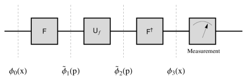
Figure 1: Single-mode quantum circuit implementing the continuous-variable Deutsch–Jozsa algorithm AHS09 .

The encoded position sinc function has unbounded extent, and analysis of the optimum position measurement window reveals an uncertainly relationship AHS09 between the measurement window $\delta$ and the encoding length $P$ expressed as

$$P\delta=\frac{\pi}{2}.$$ (5)

As a result, the single-mode continuous variable algorithm is necessarily probabilistic AHS09 and has single-query success probability

$$\text{Pr}^{\bot}_{\checkmark}=0.61.$$ (6)

Here we demonstrate that this single query success probability may be improved upon by using a Gaussian wave function as algorithm input.

II.3 Single Mode Continuous Variable Algorithm with Gaussian States

The sinc function employed as algorithm input in AHS09 cannot be readily created in the laboratory. Here we are inspired by the ability to create and manipulate physical states of light in the laboratory using the tools of quantum optics. In particular, we employ coherent states, which may by represented by Gaussian wave functions, as the input states to our algorithm.

The method of coherent states is well established and one feature is that the coherent states are overcomplete Ar72 ; Pe72 . High quality lasers generate light fields that are coherent Le97 . The vacuum state is a displaced coherent state and as such has the same quantum noise properties. Coherent states are usually expressed as the ket $\left|\alpha\right\rangle$ with $\alpha=x_{0}+{\rm{i}}p_{0}$ to reflect that it is a state that is shifted from the vacuum by the magnitude $|\alpha|$. Similarly, the vacuum is usually expressed simply as the ket $|0\rangle$.

In the position representation, the coherent state of laser light may be expressed as

$$\phi(x;\alpha)=\left\langle x|\alpha\right\rangle=\frac{e^{-\frac{1}{2}\left[(x-x_{0})^{2}-2{\rm{i}}p_{0}x+{\rm{i}}p_{0}x_{0}\right]}}{\sqrt[4]{\pi}},$$ (7)

where $x_{0}=p_{0}=0$ corresponds to the vacuum state. From the perspective of our quantum algorithm, the displaced vacuum behaves no differently than the vacuum itself. Therefore for notational simplicity, we chose to use the position representation of the vacuum,

$$\left\langle x|0\right\rangle=\frac{e^{-\frac{x^{2}}{2}}}{\sqrt[4]{\pi}},$$ (8)

as the starting-point state for our algorithm.

Quantum optics has many tools that allow for the manipulation of light. Of interest in our algorithm is light squeezing, where quantum uncertainties are redistributed altering the shape of the distribution. The squeezing operator is given in Le97 as

$$\hat{S}(\zeta)=\exp\left(\frac{\zeta}{2}\left(\hat{a}^{2}-\hat{a}^{{\dagger}2}\right)\right),$$ (9)

where $\hat{a}=\hat{x}+{\rm{i}}\hat{p}$ is the annihilation operator and $\hat{a}^{{\dagger}}=\hat{x}-{\rm{i}}\hat{p}$ is the creation operator. The quadratures $\hat{x}$ and $\hat{p}$ are regarded as the position and momentum of the harmonic oscillator, and the quantity $\zeta$ is referred to as the squeezing parameter Le97 .

In Dirac notation, the squeezed vacuum state may be expressed as

$$|\phi_{0}\rangle=\hat{S}(\zeta)|0\rangle.$$ (10)

In our analysis, we use the standard deviation $\sigma=e^{-\zeta}$ to represent the effect of the squeezing operator on our function representation of a Gaussian state.

We employ the squeezed vacuum as the input state to our algorithm, which we represent in function notation as

$$\phi_{0}(x;\sigma) =\langle x|\hat{S}(\zeta)|0\rangle$$

$$=\frac{e^{-\frac{x^{2}}{2\sigma^{2}}}}{\sqrt[4]{\pi}\sqrt{\sigma}}.$$ (11)

The subscript zero identifies this state as the algorithm input state represented by the leftmost vertical line in Fig. (1). We prove that the algorithm with this Gaussian input state has improved single-query success probability over the algorithm employing orthogonal states as input.

Theorem 1.

Using the single-mode quantum circuit given in Fig. 1 with the coherent state given by Eq. (II.3) as algorithm input and employing sharp information cutoff, the single-query success probability $\Pr^{\sharp}_{\checkmark}>\Pr^{\bot}_{\checkmark}$ is greater than the single-query success probability $\text{Pr}^{\bot}_{\checkmark}$ obtained using orthogonal states given by Eq. (6).

III Bounding the Query Complexity of the Single Mode Algorithm with Gaussian Input States

The continuous-variable quantum algorithm using orthogonal states solves Problem 1 with exponentially small error probability $1/(2^{m})$ in a linear number of queries $\Theta(m)$ AHS09 . This query complexity is dependent on the single-query success probability $\Pr^{\bot}_{\checkmark}$, which is a measure of the maximum achievable separation between the probability that the encoded string is a balanced string versus a constant string. Here, where the input is a Gaussian state, we demonstrate that the key parameters affecting this separation are the encoding width, the spread of the Gaussian wave function and the width of the measurement window. We vary these parameters and discover their optimum values in our proof of Theorem 1.

III.1 Encoding Information into Gaussian States

With reference to Fig. 1, the first step of the algorithm is to take the Fourier transform AHS09 of the input state $\phi_{0}(x;\sigma)$ giving

$$\tilde{\phi}_{1}(p\,;\sigma)=\frac{e^{-\frac{1}{2}p^{2}\sigma^{2}}\sqrt{\sigma}}{\sqrt[4]{\pi}}.$$ (12)

The next step has the oracle $\mathsf{U}_{f}$ modulate the momentum Gaussian with the pulse train that represents the encoding of the $N$-bit string $z$.

The modulated momentum wave function is

$$\tilde{\phi}_{2}(p)=\tilde{\phi}_{z}^{(N)}(p\,;\sigma,P)=\eta f_{z}^{(N)}(p;P)\tilde{\phi}_{1}(p\,;\sigma),$$ (13)

where we have labelled the state with all relevant parameters. Descriptions of the elements of this equation follow. The modulating square-wave encoded with the $N$-bit string $z$ is

$$f_{z}^{(N)}(p;P)=\sum_{i=0}^{N-1}(-1)^{z_{i}}\sqcap_{i}^{(N)}(p;P),$$ (14)

where the definition of the momentum bins given in AHS09 is repeated here as

$$\sqcap_{i}^{(N)}(p;P)=\left\{\begin{array}[]{ll}1,&\frac{p}{P}\in\left[-\left(1-2\frac{N-1-i}{N}\right),-\left(1-2\frac{N-i}{N}\right)\right]\\ 0,&\text{otherwise.}\end{array}\right.$$ (17)

Note that the modulating function has the effect of chopping off the tails of the momentum Gaussian outside $\pm P$ thus truncating the Hilbert space.

The normalization factor, $\eta$, of the chopped distribution is calculated as

$$\int_{-\infty}^{\infty}\left|\tilde{\phi}_{z}^{(N)}(p;\sigma,P)\right|^{2}\mathrm{d}p=\text{erf}(P\sigma),$$ (18)

where the error function is $\text{erf}(w)=\frac{2}{\sqrt{\pi}}\int_{0}^{w}e^{-t^{2}}dt$, and

$$\eta=1/\sqrt{\text{erf}(P\sigma)}.$$ (19)

The penultimate step is to take the inverse Fourier transform of this encoded momentum state.

The encoded position state is thus expressed as

$$\phi_{3}(x)=\phi_{z}^{(N)}(x;\sigma,P)=\frac{\eta\,\text{e}^{-\frac{x^{2}}{2\sigma^{2}}}}{2\sqrt[4]{\pi}\sqrt{\sigma}}\,M^{(N)}_{z}(x;\sigma,P).$$ (20)

The effect of the encoded information is completely captured in the position modulating term

$$M^{(N)}_{z}(x;\sigma,P)= \sum_{j=1}^{N}(-1)^{z_{j}}\left[\text{erf}\left(\frac{\vartheta_{j}\sigma^{2}+{\rm i}x}{\sqrt{2}\sigma}\right)\right.$$

$$-\left.\text{erf}\left(\frac{\vartheta_{j-1}\sigma^{2}+{\rm i}x}{\sqrt{2}\sigma}\right)\right],$$ (21)

where

$$\vartheta_{j}=P\left(\frac{2j-N}{N}\right).$$ (22)

The final step is the measurement step.

We follow the same approach taken in AHS09 and calculate the probability of detecting a particular wave function in the interval $\pm\delta$ as

$$\Pr\left[\phi_{z}^{(N)}(x;\sigma,P)\right]=\int_{-\delta}^{\delta}\left|\phi_{z}^{(N)}(x;\sigma,P)\right|^{2}\text{d}x.$$ (23)

Since the wave function may be encoded with a constant string or a balanced string, we need to determine the optimal value of $\delta$ that maximizes our ability to distinguish between these cases. Our approach is to determine which balanced functions dominate all other balanced functions in the measurement window.

We begin by defining three pairs of $N$-bit strings: the antisymmetric balanced (AB) strings, the symmetric balanced (SB) strings and the constant (C) strings as

AB $$\in\left\{\underbrace{0\cdots 0}_{N/2}\underbrace{1\cdots 1}_{N/2},\underbrace{1\cdots 1}_{N/2}\underbrace{0\cdots 0}_{N/2}\right\},$$ (24)

SB $$\in\left\{\underbrace{0\cdots 0}_{N/4}\underbrace{1\cdots 1}_{N/2}\underbrace{0\cdots 0}_{N/4},\underbrace{1\cdots 1}_{N/4}\underbrace{0\cdots 0}_{N/2}\underbrace{1\cdots 1}_{N/4}\right\},$$ (25)

C $$\in\left\{\underbrace{0\cdots 0}_{N},\underbrace{1\cdots 1}_{N}\right\}.$$ (26)

Note that the constant stings have zero bit transitions, the antisymmetric balanced strings have one bit transition, and the symmetric balanced strings have two transitions. All other balanced strings have two or greater transitions.

It is insightful to analyze the modulating term given by Eq. (21) for $x=0$, which we express as

$$M^{(N)}_{z}(0;\sigma,P) =\sum_{j=1}^{N}(-1)^{z_{j}}\left[\text{erf}\left(\frac{\vartheta_{j}\sigma}{\sqrt{2}}\right)-\text{erf}\left(\frac{\vartheta_{j-1}\sigma}{\sqrt{2}}\right)\right].$$ (27)

We use the anti-symmetric property of the error function $\text{erf}(a)=-\text{erf}(-a)$, and the property that $\text{erf}(0)=0$. We also use the facts that $\vartheta_{N}=P$, $\vartheta_{N}/2=0$ and $\vartheta_{j}=-\vartheta_{N-j}$ for $j=0,1,\ldots,N$ in determining the following results.

For the constant case, all the terms cancel except the first and last, and we have

$$M^{(N)}_{z\in\text{C}}(0;\sigma,P) =\pm\left[\text{erf}\left(\frac{\vartheta_{N}\sigma}{\sqrt{2}}\right)-\text{erf}\left(\frac{\vartheta_{0}\sigma}{\sqrt{2}}\right)\right]$$

$$=\pm 2\,\text{erf}\left(\frac{P\sigma}{\sqrt{2}}\right).$$ (28)

For the antisymmetric balanced case, all the terms cancel and we have

$$M^{(N)}_{z\in AB}(0;\sigma,P) =\pm\left[\text{erf}\left(\frac{\vartheta_{N}\sigma}{\sqrt{2}}\right)+\text{erf}\left(\frac{\vartheta_{0}\sigma}{\sqrt{2}}\right)\right]$$

$$=0.$$ (29)

For the symmetric case we have

$$M^{(N)}_{z\in SB}(0;\sigma,P) =\pm\left[2\,\text{erf}\left(\frac{P\sigma}{\sqrt{2}}\right)-4\,\text{erf}\left(\frac{P\sigma}{2\sqrt{2}}\right)\right].$$ (30)

Here the sum is non-zero except for in the limiting case where $P\sigma\rightarrow 0$.

It is apparent from the results of Eqs. (29) and (30) that there are different classes of balanced functions. Some balanced functions are only non-zero at $x=0$ in the limit as $\sigma$ goes to zero, and some balanced functions are zero at $x=0$ for all values of $\sigma$. We need to determine which balanced functions are the two functions that dominate the measurement region.

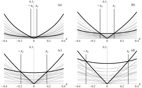
Figure 2: Plots of the magnitude of the position modulation function $\left|M^{(8)}_{z}(x;\sigma,1)\right|$ given by Eq. (20) for (a) $\sigma=0.4$, (b) $\sigma=0.6$, (c) $\sigma=0.8$, and (d) $\sigma=1.0$. For $\left|x\right|<x_{c}$, the symmetric balanced function (bold) dominates all other balanced functions, and for $\left|x\right|>x_{c}$, the antisymmetric balanced function (bold) dominates all other balanced functions.

In Appendix A, we prove that the magnitude of the position modulation function $\left|M^{(N)}_{z}(x;\sigma,1)\right|$ given by Eq. (20) and subject to the balanced condition $\sum_{i=1}^{N}(-1)^{z_{i}}=0$, is maximized by either the antisymmetric balanced function given by Eq. (24) or the symmetric balanced function given by Eq. (25). For $N=8$, the situation is presented in Fig. 2, where it be seen that the actual dominating function is dependent on the value of $\sigma$.

In Fig. 2, the crossover point is drawn and is approximated in Appendix A as

$$x_{c}\approx\frac{P\sigma^{2}}{(4-P^{2}\sigma^{2})}.$$ (31)

For $|x|<x_{c}$, the symmetric balanced function (shown in bold) dominates, and for $|x|>x_{c}$, the antisymmetric balanced function (shown in bold) dominates. All remaining balanced functions, of which there are a total of $\binom{8}{4}=70$ are depicted as light gray lines in Fig. 2. We use these results to complete the proof of Theorem 1.

III.2 Proof of Theorem 1

We need to maximize the separation between detecting a balanced string and a constant string. To this end, we define the following quantities

$$\Delta_{\text{AB}}(\sigma,P,\delta)=\left|\Pr\left[\phi_{z\in\text{C}}^{(N)}\right]-\Pr\left[\phi_{z\in\text{AB}}^{(N)}\right]\right|,$$ (32)

and

$$\Delta_{\text{SB}}(\sigma,P,\delta)=\left|\Pr\left[\phi_{z\in\text{C}}^{(N)}\right]-\Pr\left[\phi_{z\in\text{SB}}^{(N)}\right]\right|,$$ (33)

where for brevity, we have suppressed the arguments in Eq. (23). The single-query success probability is defined in these terms as

$$\text{Pr}_{\checkmark}^{\sharp}=\min\left[\Delta_{\text{AB}}(\sigma,P,\delta),\Delta_{\text{SB}}(\sigma,P,\delta)\right].$$ (34)

This expression assumes that either the antisymmetric or the symmetric balanced strings dominate all other balanced strings in the region $\pm\delta$ as presented in the previous subsection and proved in Appendix A. We seek to determine the values of $\delta$ and $\sigma$ that maximize the separation between these two probabilities.

With $\Delta_{\text{AB}}(\delta,\sigma,P)$ defined in Eq. (32), we set $\Delta_{\text{AB}}^{\prime}(\delta,\sigma,P)=\frac{\partial}{\partial\delta}\Delta_{\text{AB}}(\delta,\sigma,P)$, which gives us

$$\Delta_{\text{AB}}^{\prime}(\delta,\sigma,P)=$$

$$\frac{e^{-\frac{\delta^{2}}{\sigma^{2}}}}{2\sqrt{\pi}\sigma\,\text{erf}(P\sigma)}\left[\text{erf}\left(\frac{P\sigma^{2}-{\rm{i}}\delta}{\sqrt{2}\sigma}\right)^{2}+\text{erf}\left(\frac{P\sigma^{2}+{\rm{i}}\delta}{\sqrt{2}\sigma}\right)^{2}\right.$$

$$\left.+\,2\,\text{erf}\left(\frac{P\sigma^{2}-{\rm{i}}\delta}{\sqrt{2}\sigma}\right)\text{erf}\left(\frac{{\rm{i}}\,\delta}{\sqrt{2}\sigma}\right)+2\,\text{erf}\left(\frac{{\rm{i}}\,\delta}{\sqrt{2}\sigma}\right)^{2}\right.$$

$$\left.+\,2\,\text{erf}\left(\frac{P\sigma^{2}+{\rm{i}}\delta}{\sqrt{2}\sigma}\right)\text{erf}\left(\frac{{\rm{i}}\,\delta}{\sqrt{2}\sigma}\right)\right].$$ (35)

It suffices to set $\Delta_{\text{AB}}^{\prime}(\delta,\sigma,P)=0$ to maximize the separation. Before doing so, we elect to simplify Eq. (III.2) by ‘normalizing’ the standard deviation $\sigma$ and the measurement ‘length’ $\delta$ with respect to the encoding ‘length’ $P$.

We assume that the uncertainty relation AHS09 remains true up to a constant. We express this as

$$P\delta=\bar{\delta}.$$ (36)

This assumption and analysis of the error function arguments of Eq. (III.2) result in a similar uncertainty relationship between $P$ and $\sigma$, which we express as

$$P\sigma=\bar{\sigma}.$$ (37)

Making the substitutions given by Eq. (36) and Eq. (37) into Eq. (III.2) and setting it to 0 results in the following expression

$$\Delta_{\text{AB}}^{\prime}\left(\bar{\delta},\bar{\sigma}\right)=0$$

$$=\left[\text{erf}\left(\frac{\bar{\sigma}^{2}-{\rm{i}}\,\bar{\delta}}{\sqrt{2}\bar{\sigma}}\right)^{2}+\text{erf}\left(\frac{\bar{\sigma}^{2}+{\rm{i}}\,\bar{\delta}}{\sqrt{2}\bar{\sigma}}\right)^{2}\right.$$

$$\left.+\,2\,\text{erf}\left(\frac{\bar{\sigma}^{2}-{\rm{i}}\,\bar{\delta}}{\sqrt{2}\bar{\sigma}}\right)\text{erf}\left(\frac{{\rm{i}}\,\bar{\delta}}{\sqrt{2}\bar{\sigma}}\right)+2\,\text{erf}\left(\frac{{\rm{i}}\,\bar{\delta}}{\sqrt{2}\bar{\sigma}}\right)^{2}\right.$$

$$\left.+\,2\,\text{erf}\left(\frac{\bar{\sigma}^{2}+{\rm{i}}\,\bar{\delta}}{\sqrt{2}\bar{\sigma}}\right)\text{erf}\left(\frac{{\rm{i}}\,\bar{\delta}}{\sqrt{2}\bar{\sigma}}\right)\right].$$ (38)

Note that the variables $\bar{\sigma}$ and $\bar{\delta}$ are, in some sense the ‘normalized’ Gaussian standard deviation $\sigma$ and the measurement width $\delta$, ‘scaled’ by the momentum ‘length’ $P$.

Eq. (III.2) is dependent on the two variables, $\bar{\delta}$ and $\bar{\sigma}$ and is thus insufficient to find the global optimum values of $\bar{\sigma}$ and $\bar{\delta}$. We obtain the needed constraint from the similar equation derived from the symmetric balanced function. Following the same steps we did in Eq. (III.2) and Eq. (III.2), we obtain the following expression

$$\Delta_{\text{\tiny{SB}}}^{\prime}\left(\bar{\delta},\bar{\sigma}\right)=0$$

$$=\left[\text{erf}\left(\frac{\bar{\sigma}^{2}-i\bar{\delta}}{2\sqrt{2}\bar{\sigma}}\right)+\text{erf}\left(\frac{\bar{\sigma}^{2}+i\bar{\delta}}{2\sqrt{2}\bar{\sigma}}\right)\right]$$

$$\times\left[-\text{erf}\left(\frac{{}^{2}-i\bar{\delta}}{2\sqrt{2}\bar{\sigma}}\right)+\text{erf}\left(\frac{\bar{\sigma}^{2}-i\bar{\delta}}{\sqrt{2}\bar{\sigma}}\right)\right.$$

$$-\left.\text{erf}\left(\frac{\bar{\sigma}^{2}+i\bar{\delta}}{2\sqrt{2}\bar{\sigma}}\right)+\text{erf}\left(\frac{\bar{\sigma}^{2}+i\bar{\delta}}{\sqrt{2}\bar{\sigma}}\right)\right].$$ (39)

We solve Eqs. (III.2) and (III.2) simultaneously to establish the optimum values of the measurement lengths $\bar{\delta}_{\text{AB}}$ and $\bar{\delta}_{\text{SB}}$ in terms of the normalized standard deviation $\bar{\sigma}$.

Figure 3: Plots of $\left|\phi^{(N)}_{z}(x;\sigma,1)\right|^{2}$ for $z\in\{\text{AB},\text{SB},\text{C}\}$ (solid, dotted, dashed respectively) for: (a) $\sigma=1.67$, (b) $\sigma=2.11$, (c) $\sigma=2.5$, and (d) $\sigma=3.0$. The solid vertical lines in all four sub-plots correspond to $\Delta^{\prime}_{\text{\tiny{AB}}}\left(\bar{\delta},\bar{\sigma}\right)=0$, and the dashed vertical lines correspond to $\Delta^{\prime}_{\text{\tiny{SB}}}\left(\bar{\delta},\bar{\sigma}\right)=0$. Note that a) corresponds to the values that optimize the single-query success probability.

In Fig. 3, we plot the distributions $|\phi^{(N)}_{z}(x;\sigma,P)|^{2}$ for $z\in\{\text{AB},\text{SB},\text{C}\}$ for several values of $\sigma$. We also plot vertical lines corresponding to the values of $\bar{\delta}$ corresponding to $\Delta^{{}^{\prime}}_{\text{\tiny{AB}}}=0$ and $\Delta^{{}^{\prime}}_{\text{\tiny{SB}}}=0$. Note that there are values of the normalized parameters $\bar{\sigma}$ and $\bar{\delta}$ where $\Delta^{{}^{\prime}}_{\text{\tiny{AB}}}\left(\bar{\delta},\bar{\sigma}\right)=0$, and $\Delta^{{}^{\prime}}_{\text{\tiny{SB}}}\left(\bar{\delta},\bar{\sigma}\right)=0$ simultaneously. This situation occurs where $\bar{\delta}\approx 2.30$ and $\bar{\sigma}\approx 2.11$ and is depicted in Fig. 3(b).

However, these values do not optimize the success probability since

$$\Delta_{\text{\tiny{AB}}}(2.30,2.11)\approx 0.68,\,\,\text{and}$$

$$\Delta_{\text{\tiny{SB}}}(2.30,2.11)\approx 0.54.$$ (40)

Lack of optimality is manifest in the lower of the two above values, which is less than single-query success probability for the orthogonal case $\text{Pr}_{\checkmark}^{\bot}\approx 0.61$.

Increasing the value of $\bar{\sigma}$ further serves to increase $\Delta_{\text{\tiny{AB}}}\left(\bar{\delta},\bar{\sigma}\right)$ and decrease $\Delta_{\text{\tiny{SB}}}\left(\bar{\delta},\bar{\sigma}\right)$, which worsens the success probability. Reducing the value of $\bar{\sigma}$ brings them together. The quantity $\Delta_{\text{\tiny{AB}}}\left(\bar{\delta},\bar{\sigma}\right)$ thus takes on its maximum value when

$$\Delta^{\prime}_{\text{\tiny{AB}}}\left(\bar{\delta},\bar{\sigma}\right)=0$$ (41)

subject to the constraint

$$\Delta_{\text{\tiny{AB}}}\left(\bar{\delta},\bar{\sigma}\right)=\Delta_{\text{\tiny{SB}}}\left(\bar{\delta},\bar{\sigma}\right).$$ (42)

This occurs at a value of  $\bar{\delta}{\text{\tiny{AB}}}\approx 2.01$ and $\bar{\sigma}\approx 1.67$. Optimality is manifest since

$$\Delta_{\text{\tiny{AB}}}\left(\bar{\delta},\bar{\sigma}\right)=\Delta_{\text{\tiny{SB}}}\left(\bar{\delta},\bar{\sigma}\right)\approx 0.68.$$ (43)

The optimal situation is depicted in Fig. 3(a).

For $P=1$, we express the optimal parameters as

$$\delta^{\sharp}\approx 2.01,$$ (44)

and

$$\sigma^{\sharp}\approx 1.67.$$ (45)

For these values, the single query success probability of the Gaussian model with sharp information cut-off model is

$$\text{Pr}_{\checkmark}^{\sharp}\approx 0.68.$$ (46)

This upper bound is approximately 10$\%$ greater than that shown for the model employing orthogonal states AHS09 , where $\text{Pr}_{\checkmark}^{\bot}\approx 0.61$ and $\delta^{\bot}=\frac{\pi}{2}$.

At first glance, the increase in single-query success probability of the Gaussian case over the orthogonal case appears somewhat surprising. The Gaussian wave functions are coherent states and therefore non-orthogonal Pe72 . Intuitively, the orthogonal states should be optimal especially given that the finite extent of the momentum wave functions provides a natural fit for encoding finite infirmation.

Upon closer inspection however, we see that the improvement results from the ability to ‘tune’ the Gaussian spread, represented by $\sigma$, to match the encoding length $P$. No such ‘tuning’ is possible with the finite states. We depict this in Fig. 4(a) for the constant case with $P=1$ and optimal $\sigma^{\sharp}=1.67$. We see that the encoded momentum Gaussian wave function is on average narrower than the orthogonal pulse wave function. Since the momentum and position wave functions are Fourier transform pairs, narrowing of one results in broadening of the other.

The subsequent broadening of the encoded Gaussian wave functions results in a wider optimal measurement window $\delta^{\sharp}>\delta^{\bot}$. This leads to a greater single-query success probability and is represented by the shaded regions in Fig. 4(b). The larger dark gray region corresponds to the single-query success probability offered by the Gaussian wave functions. We thus conclude that the increased success probability is achieved through the extra degree of freedom afforded by $\sigma$. For $P=1$, this requires that the input state be squeezed to $\sigma\approx 1.67$.

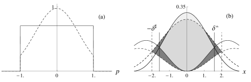
Figure 4: Comparison between the orthogonal (solid) and the Gaussian (dashed) wave functions. The amplitude of the encoded momentum functions for the constant case is depicted in (a). The respective algorithm success probabilities are depicted by the shaded regions of (b), where light gray correspond to the orthogonal case and dark gray corresponds to the Gaussian case. Medium grey corresponds to the region of overlap. Note that the encoded momentum Gaussian is on average narrower than the orthogonal pulse, which results in respectively broader position wave functions.

IV Conclusions

We have shown that a simple-harmonic-oscillator quantum computer solving oracle decision problems performs better using non-orthogonal Gaussian wave functions as the algorithm input rather than the orthogonal top-hat wave functions. We have also shown that the limiting case of the Gaussian model for $\sigma\rightarrow 0$ and non-zero $P$ corresponds to the model employing orthogonal states. In both cases, the computational bases are orthogonal, and encoding takes place in the momentum domain and information processing and measurement take place in the dual position domain. Also in both cases, the single-query success probability is dependent on the maximum separation between the position wave function encoded with the constant string and the position wave function encoded with the worst-case balanced string, which is the antisymmetric balanced string.

In the orthogonal case, $N$-bit strings are uniquely encoded into the computational basis formed by the top-hat functions, and the overall-width of the encoded string is set by the encoding length $P$. In the dual position domain, the encoded string is represented by a sum of $N$ equi-angularly spaced, equi-length phasors multiplied by a sinc function. The rate at which the constant sinc function falls off its peak and the rate that the antisymmetric balanced sinc function rises from its minimum sets the size of the optimum position domain measurement window. Thus the optimum position domain measurement is set by sharpness of the sinc function, which is dependent on the encoding length only.

In the Gaussian case, $N$-bit strings are uniquely encoded into the computational basis formed by more complicated Gaussian-modulated basis states. The overall-width of the encoded string is again set by the encoding length $P$, but it is also shaped by the Gaussian spread $\sigma$. In the dual position domain, the encoded string is represented by a sum of non equi-angularly spaced and non equi-length phasors multiplied by a Gaussian function. The rate at which the constant encoded function falls off its peak and the rate that the antisymmetric balanced function rises from its minimum is governed by both the Gaussian spread $\sigma$ and the encoding length $P$. More importantly, the rate set by the optimal values of $\sigma$ and $P$ is more gradual than that achievable in the orthogonal case allowing for greater separation between the two probabilities.

We thus conclude that the Gaussian allows for an improved trade-off between encoding, processing and measuring of the information. Encoding takes place in the momentum domain, and the Gaussian takes better advantage of the space available to encode the information. Correspondingly, information processing and measurement take place in the dual position domain. The Gaussian-encoded position wave function enables a wider measurement window, which means more of the encoded information is available for distinguishing between a wave function encoded with a constant string and a wave function encoded with the worst-case balanced string.

Appendix A Proofs of dominance of symmetric and antisymmetric balanced functions

In this appendix we prove that the symmetric and the antisymmetric balanced functions maximize the magnitude of $\left|M^{(N)}_{z}(x;\sigma,1)\right|$ given by Eq. (20) subject to the balanced condition $\sum_{i=1}^{N}(-1)^{z_{i}}=0$ in three Lemmas.

Lemma 1.

For the region $|x|\leq\pi$ with $\sigma=0$ and subject to the balanced condition $\sum_{j=1}^{N}(-1)^{z_{j}}=0$, $\max\left|\phi_{z}^{(N)}(x;\sigma,P)\right|$ occurs for $z\in\{\text{AB}\}$.

Proof.

We prove this Lemma by showing that, in the limiting case where $\sigma\rightarrow 0$, the encoded position wave function given in Eq. (20) becomes the same as the encoded orthogonal wave function analyzed in AHS09 . In that case, it is proved that the antisymmetric balanced function dominates all other balanced wave functions in the region of interest.

We begin by defining the quantity

$$A_{k}(x,\sigma)=\text{erf}\left(\frac{\frac{2Pk}{N}\sigma^{2}-{\rm i}x}{\sqrt{2}\sigma}\right)-\text{erf}\left(\frac{\frac{2P(k-1)}{N}\sigma^{2}-{\rm i}x}{\sqrt{2}\sigma}\right)$$ (47)

for $k=1,...,N/2$. We use this term here and in later Lemmas. For ease of understanding the antisymmetric features of this term, we have elected to change the counting variable in the term $\vartheta_{j}$ given in Eq. (22) from $j$ to $k$, where $j=k+N/2$. We express the $k^{\rm{th}}$ term of the encoded position wave function given by Eq. (20) in terms of this quantity as

$$\phi_{z}^{(k)}(x;\sigma,P) =\pm\frac{\eta\,\text{e}^{-\frac{x^{2}}{2\sigma^{2}}}}{2\sqrt[4]{\pi}\sqrt{\sigma}}A_{k}(x,\sigma)$$ (48)

where the $\pm$ represents the effect of the bit $(-1)^{z_{k}}$. We represent this quantity as the phasor

$$\phi_{z}^{(k)}(x;\sigma,P) =\pm R_{k}(x;\sigma,P)\exp\left[{\rm i}\varphi_{k}(x;\sigma,P)\right],$$ (49)

to align with the description of the orthogonal case.

The phasor magnitude is expressed

$$R_{k}(x;\sigma,P)=\left|\frac{\eta\,\text{e}^{-\frac{x^{2}}{2\sigma^{2}}}}{2\sqrt[4]{\pi}\sqrt{\sigma}}A_{k}\right|,$$ (50)

and the argument is

$$\varphi_{k}(x;\sigma,P)=\arctan\left(\frac{\text{Im}\left[A_{k}\right]}{\text{Re}\left[A_{k}\right]}\right),$$ (51)

where we have suppressed the arguments of $A_{k}$ for the sake of brevity.

The quantities $R_{k}(x;\sigma)$ and $\varphi_{k}(x;\sigma)$ are too opaque to understand limiting behaviour, so we use Taylor series analysis to gain insight. The Taylor series representation of angle $\varphi_{k}(x;\sigma)$ given by Eq. (51) is expressed

$$\varphi_{k}(x;\sigma) =\frac{(2k-1)x}{N}-\frac{(2k-1)x\sigma^{2}}{3N^{3}}+\frac{2(2k-1)x\sigma^{4}}{45N^{5}}$$

$$+O\left(x\sigma^{6}\right)+O\left(x^{3}\sigma^{2}\right)$$ (52)

where for $\sigma=0$, we have

$$\varphi_{k}(x;0) =\frac{(2k-1)x}{N},$$ (53)

which presents an equiangular separation between subsequent phasors.

Similarly the Taylor series for magnitude given by Eq. (50) is expressed

$$R_{k}(x;\sigma) =\frac{1}{N\sqrt{\pi}}-\frac{x^{2}}{6N^{3}\sqrt{\pi}}+\frac{\left(N^{2}-12(k-1)k-4\right)\sigma^{2}}{6N^{3}\sqrt{\pi}}$$

$$+\frac{\left(-5N^{2}+60(k-1)k+24\right)\sigma^{2}x^{2}}{180N^{5}\sqrt{\pi}}+O\left(x^{4}\sigma^{4}\right).$$ (54)

For $\sigma=0$, this gives

$$R_{k}(x;0) =\frac{\sqrt{P}}{N\sqrt{\pi}}-\frac{P^{5/2}x^{2}}{6N^{3}\sqrt{\pi}}+\cdots+\frac{(-1)^{m}\sqrt{P}\left(\frac{Px}{N}\right)^{2m}}{N\sqrt{\pi}(2m+1)!}$$

$$=\frac{\sin{\left(Px/N\right)}}{\sqrt{P\pi}x},$$ (55)

where the last step assumes the limit $m\rightarrow\infty$.

Combining the results of Eqs. (49), (53), and  (55) gives

$$\phi_{z}^{(N)}(x;0,P)=\frac{\sin{\left(Px/N\right)}}{\sqrt{P\pi}x}\sum_{j=1}^{N}(-1)^{z_{j}}\text{e}^{\rm{i}\left(\frac{N-(2j-1)}{N}\right)Px},$$ (56)

which is the encoded orthogonal position wave function given in AHS09 . The proof given therein suffices to prove Lemma 1. ∎

Lemma 2.

For $x=0$ and $\sigma>0$ and subject to the balanced constraint $\sum_{j=1}^{N}(-1)^{z_{j}}=0$, $\max\left|\Xi_{z}^{(N)}(0;\sigma)\right|$ occurs for $z\in\{\text{SB}\}$.

Proof.

We exploit the structure of the quantity given in Eq. (47) with $x=0$ expressed as

$$A_{k}(0,\sigma)=\text{erf}\left(\frac{\frac{2k}{N}\sigma^{2}}{\sqrt{2}\sigma}\right)-\text{erf}\left(\frac{\frac{2(k-1)}{N}\sigma^{2}}{\sqrt{2}\sigma}\right).$$ (57)

Using the shorthand $A_{k}=A_{k}(0,\sigma)$, we express a set of $N$ terms in the following convenient form

$$\{A_{\frac{N}{2}},\ldots,A_{k},\ldots,A_{2},A_{1},A_{1},A_{2},\ldots,A_{k},\ldots,A_{\frac{N}{2}}\},$$ (58)

for $k=1,2,\ldots,\frac{N}{2}$. Note that the $A_{k}$ are real numbers.

We now show that $A_{k}>A_{k+1}$. We express the difference between these terms as

$$A_{k}-A_{k+1} =2\,\text{erf}\left(\frac{\sqrt{2}k\sigma}{N}\right)-\text{erf}\left(\frac{\sqrt{2}(k-1)\sigma}{N}\right)$$

$$-\text{erf}\left(\frac{\sqrt{2}(k+1)\sigma}{N}\right).$$ (59)

Showing that Eq. (59) is positive for all $k$ is equivalent to showing that

$$2\,\text{erf}(a)-\text{erf}(a+b)-\text{erf}(a-b)>0$$ (60)

for $a,b\in\mathbb{R}$ and $a,b>0$.

Over the domain $(0,\infty)$, the error function is strictly monotonically increasing with strictly monotonically decreasing slope $\frac{\text{d}}{\text{d}x}\text{erf}(x)=2e^{-x^{2}}/\sqrt{\pi}$. This means that successive increments $\delta x$ result in decreasing $\delta y=\text{erf}(\delta x)$ increments. This may be expressed as

$$\text{erf}(a)-\text{erf}(a-b)>\text{erf}(a+b)-\text{erf}(a),$$ (61)

and thus

$$2\text{erf}(a)-\text{erf}(a-b)-\text{erf}(a+b)>0,$$ (62)

which establishes that $A_{k}>A_{k+1}$.

The strategy required to maximize the sum of the $N$ terms of the set (58) subject to the balanced constraint is now clear. Since $A_{1}>A_{2}>\cdots>A_{\frac{N}{2}}$, the maximal term must contain as many of the larger terms as possible. This maximal sum is thus expressed

$$\pm 2\left(A_{1}+A_{2}+\dots+A_{\frac{N}{4}}-A_{\frac{N}{4}+1}-A_{\frac{N}{4}+2}-\dots-A_{\frac{N}{2}}\right).$$ (63)

This expression manifests the symmetric balanced (SB) function definition given in Eq. (25) thus proving the Lemma. ∎

Lemma 3.

For $|x|>0$ and $\sigma\geq 0$ and subject to the balanced condition $\sum_{j=1}^{N}(-1)^{z_{j}}=0$, $\max\left|\phi_{z}^{(N)}(x;\sigma)\right|$ occurs for either $z\in\{\text{SB}\}$ or for $z\in\{\text{AB}\}$.

Proof.

We modify the set of elements $A_{k}$ to include the imaginary components resulting from $x>0$ as

$$\left\{A^{*}_{\frac{N}{2}}(x,\sigma),\ldots,A^{*}_{1}(x,\sigma),A_{1}(x,\sigma),\dots,A_{\frac{N}{2}}(x,\sigma)\right\}.$$ (64)

We now exploit the antisymmetric property of this set. The fact that $\text{erf}(w^{*})=\text{erf}^{*}(w)$ allows us to use the notation

$$A_{k}(x,\sigma)=\alpha_{k}+\rm{i}\beta_{k},$$ (65)

and

$$A^{*}_{k}(x,\sigma)=\alpha_{k}-\rm{i}\beta_{k}$$ (66)

to capture the overall of effect of the error function having complex arguments.

The strategy to maximize the sum of the elements in the set given expression (64) subject to the balanced constraint is clear. The sum must be either purely real or purely imaginary. A complex sum reduces these achievable maximums in two ways. It causes elements to be subtracted, and it results in a vector sum rather than a liner sum.

The maximum real sum subject to the balanced constraint is

$$\sum_{k=1}^{k=N/4}A_{k}(x,\sigma)+A^{*}_{k}(x,\sigma)-\sum_{k=n/4+1}^{k=N/2}A_{k}(x,\sigma)+A^{*}_{k}(x,\sigma)$$

$$=2\left(\sum_{k=1}^{k=N/4}\alpha_{k}(x,\sigma)-\sum_{k=N/4+1}^{k=N/2}\alpha_{k}(x,\sigma)\right),$$ (67)

which is achieved for the symmetric balanced function demonstrated in Lemma 2. The maximum imaginary sum subject to the balanced constraint is

$$\sum_{k=1}^{k=N/2}A_{k}(x,\sigma)-\sum_{k=1}^{k=N/2}A^{*}_{k}(x,\sigma)$$

$$=2\rm{i}\sum_{k=1}^{k=N/2}\beta_{k}(x,\sigma),$$ (68)

which is achieved for the antisymmetric balanced function.

As $x$ increases from zero, the imaginary component of the error function increases accordingly. For small $x$, the real part still dominates and the symmetric balanced function is the balanced function with the greatest magnitude. However, there is a point where the antisymmetric balanced function takes over the dominate role. We determine the value of this crossover point, $x_{c}$, in terms of $\sigma$ and $P$ in the following.

The $N=4$ case is the simplest case which demonstrates the crossover. For this case the set is

$$\left\{A^{*}_{2}(x,\sigma),A^{*}_{1}(x,\sigma),A_{1}(x,\sigma),A_{2}(x,\sigma)\right\}.$$ (69)

The antisymmetric balanced sum is

$$\left(-A^{*}_{2}(x,\sigma)-A^{*}_{1}(x,\sigma)+A_{1}(x,\sigma)+A_{2}(x,\sigma)\right)$$

$$=\alpha_{1}+\alpha_{2}+\rm{i}(\beta_{1}+\beta_{2})-\alpha_{1}-\alpha_{2}+\rm{i}(\beta_{1}+\beta_{2})$$

$$=\rm{i}2(\beta_{1}+\beta_{2}),$$ (70)

and the symmetric balanced sum is

$$\left(-A^{*}_{2}(x,\sigma)+A^{*}_{1}(x,\sigma)+A_{1}(x,\sigma)-A_{2}(x,\sigma)\right)$$

$$=2(\alpha_{1}-\alpha_{2}).$$ (71)

The switch over thus occurs when

$$(\beta_{1}+\beta_{2})=(\alpha_{1}-\alpha_{2}),$$ (72)

for which the lowest-order Taylor approximation is

$$x_{c}\approx\frac{P\sigma^{2}}{\left(4-P^{2}\sigma^{2}\right)}.$$ (73)

For $N=8$, this crossover point from symmetric to antisymmetric dominance is plotted in Fig. 2. ∎

References

- (1) Cormen, T. H., Leiserson, C. E., Rivest, R. L., and Stein, C., Introduction to Algorithms, McGraw-Hill, Cambridge, MA, 2001.
- (2) Sipser, M., Introduction to the Theory of Computation, PWS Publishing Company, Boston, MA, 1997.
- (3) Jackson, A. S., Analog Computation, McGraw-Hill, New York, NY, 1974.
- (4) Nielsen, M. A. and Chuang, I. L., Quantum Computation and Quantum Information, Cambridge University Press, Cambridge UK, 2000.
- (5) Braunstein, S. L. and Pati, A. K., Quantum Information with Continuous Variables, Kluwer Academic Publisher, Dordrecht, NL, 2003.
- (6) Gottesman, D., Kitaev, A., and Preskill, J., “Encoding a qubit in an oscillator,” Phys. Rev., Vol. A64, 2001, pp. 012310. doi:10.1103/PhysRevA.64.012310.
- (7) Deutsch, D., “Quantum theory, the Church-Turing principle and the universal quantum compute,” Proc. R. Soc. Lond. A, Vol. 400, July 1985, pp. 97–117. doi:10.1098/rspa.1985.0070.
- (8) Deutsch, D. and Jozsa, R., “Rapid solution of problems by quantum computation,” Proc. Royal Soc. Lond. A, Vol. 439, December 1992, pp. 553–558. doi:10.1098/rspa.1992.0167.
- (9) Adcock, M. R. A., Høyer, P., and Sanders, B. C., “Limitations on continuous variable quantum algorithms with Fourier transforms,” New J. Phys., Vol. 11, 2009, pp. 103035. doi:10.1088/1367-2630/11/10/103035.
- (10) Furusawa, A., Sørensen, J. L., Braunstein, S. L., Fuchs, C. A., Kimble, H. J., and Polzik, E. S., “Unconditional quantum teleportation,” Science, Vol. 282, 1998, pp. 706–709. doi:10.1126/science.282.5389.706.
- (11) Grosshans, F. and Grangier, P., “Continuous variable quantum cryptography using coherent states,” Phys. Rev. Lett., Vol. 88, 2002, pp. 057902. doi:10.1103/PhysRevLett.88.057902.
- (12) Appel, J., Figueroa, E., Korystov, D., Lobino, M., and Lvovsky, A. I., “Quantum memory for squeezed light,” Phys. Rev. Lett., Vol. 100, 2008, pp. 093602. doi:10.1103/PhysRevLett.100.093602.
- (13) Akamatsu, D., Yokoi, Y., Arikawa, M., Nagatsuka, S., Tanimura, T., Furusawa, A., and Kozuma, M., “Ultraslow propagation of squeezed vacuum pulses with electromagnetically induced transparency,” Phys. Rev. Lett., Vol. 99, 2007, pp. 153602. doi:10.1103/PhysRevLett.99.153602.
- (14) Braunstein, S. L., “Error correction for continuous quantum variables,” Phys. Rev. Lett., Vol. 80, 1998, pp. 4084–4087. doi:10.1103/PhysRevLett.80.4084.
- (15) Eisert, J., Plenio, M. B., and Scheel, S., “Distilling Gaussian states with Gaussian operations is impossible,” Phys. Rev. Lett., Vol. 89, 2002, pp. 137903. doi:10.1103/PhysRevLett.89.137903.
- (16) Bartlett, S. D., Sanders, B. C., Braunstein, S. L., and Nemoto, K., “Efficient classical simulation of continuous variable quantum information processes,” Phys. Rev. Lett., Vol. 88, 2002, pp. 09704. doi:10.1103/PhysRevLett.88.097904.
- (17) Bartlett, S. D. and Sanders, B. C., “Efficient classical simulation of optical quantum information circuits,” Phys. Rev. Lett., Vol. 89, 2002, pp. 207903. doi:10.1103/PhysRevLett.89.207903.
- (18) Cerf, N., Høyer, P., Magnin, L., and Sanders, B. C., “Quantum algorithms with continuous variables for black box problems,” 3rd International Workshop on Physics and Computation (PC 2010), 2010, Conference proceedings available at http://www.pc2010.uac.pt/.
- (19) Leonhardt, U., Measuring the Quantum State of Light, Cambridge University Press, Cambridge UK, 1997.
- (20) Cleve, R., Ekert, A., Macchiavello, C., and Mosca, M., “Quantum algorithms revisited,” Proc. R. Soc. Lond. A, Vol. 454, September 1998, pp. 339–354. doi:10.1098/rspa.1998.0164.
- (21) Adcock, M. R. A., Høyer, P., and Sanders, B. C., “Quantum computation with coherent spin states and the close Hadamard problem,” Available at http://arxiv.org/abs/1112.1446.
- (22) Arrechi, F. T., Courtens, E., Gilmore, R., and Thomas, H., “Atomic coherent states in quantum optics,” Phys. Rev., Vol. A6, 1972, pp. 2211–2237. doi:10.1103/PhysRevA.6.2211.
- (23) Perelomov, A., Generalized Coherent States and their Applications, Springer-Verlag, New York, NY, 1972.