Underscreened Kondo effect in $S=1$ magnetic quantum dots:
Exchange, anisotropy and temperature effects

Abstract

We present a theoretical analysis of the effects of uniaxial magnetic anisotropy and contact-induced exchange field on the underscreened Kondo effect in $S=1$ magnetic quantum dots coupled to ferromagnetic leads. First, by using the second-order perturbation theory we show that the coupling to spin-polarized electrode results in an effective exchange field $B_{\rm eff}$ and an effective magnetic anisotropy $D_{\rm eff}$. Second, we confirm these findings by using the numerical renormalization group method, which is employed to study the dependence of the quantum dot spectral functions, as well as quantum dot spin, on various parameters of the system. We show that the underscreened Kondo effect is generally suppressed due to the presence of effective exchange field and can be restored by tuning the anisotropy constant, when $|D_{\rm eff}|=|B_{\rm eff}|$. The Kondo effect can also be restored by sweeping an external magnetic field, and the restoration occurs twice in a single sweep. From the distance between the restored Kondo resonances one can extract the information about both the exchange field and the effective anisotropy. Finally, we calculate the temperature dependence of linear conductance for the parameters where the Kondo effect is restored and show that the restored Kondo resonances display a universal scaling of $S=1/2$ Kondo effect.

I Introduction

Although manifestation of the Kondo effect in nanoscopic systems of spin $S>1/2$ has been the subject of extensive experimental and theoretical studies for more than a decade, Scott and Natelson (2010); Sasaki et al. (2000); Schmid et al. (2000); van der Wiel et al. (2002); Kogan et al. (2003) it is still attracting considerable attention. From the experimental point of view, this was triggered by a rapid development of techniques Meier et al. (2008); Ternes et al. (2009); Wiebe et al. (2011) allowing for controlled preparation and investigation of single magnetic impurities, such as atoms and molecules, placed on a surface Zhao et al. (2005); Voss et al. (2008); Mannini et al. (2010); Prüser et al. (2011); Kahle et al. (2011) or captured in a junction. Heersche et al. (2006); Jo et al. (2006); Roch et al. (2008); Zyazin et al. (2010); Florens et al. (2011); Vincent et al. (2012); Burzurı et al. (2012) Furthermore, an important issue is the interaction of individual large-spin atoms or molecules with the environment, which may contribute to a magnetic anisotropy.Boča (1999); Gambardella et al. (2003); Hirjibehedin et al. (2007); Wende et al. (2007); Brune and Gambardella (2009); Gambardella et al. (2009); Serrate et al. (2010) A significant uniaxial magnetic anisotropy, in turn, results in an energy barrier for switching the molecules’s spin between two metastable states – the feature indispensable for potential applications in information storage technologies. Mannini et al. (2009); Loth et al. (2010) Interestingly enough, the magnetic state of such a system can in principle be controlled by means of spin-polarized currents, Timm and Elste (2006); Misiorny and Barnaś (2007, 2009); Misiorny et al. (2009) which has already been experimentally confirmed. Loth et al. (2010)

In order to be able to exploit advantageous features stemming from the presence of magnetic anisotropy, a possibility of its external control would be very desirable. Indeed, several experiments have so far confirmed the feasibility of such a control. The most straightforward way to modify the magnetic anisotropy of an adatom is just to change its nearest atomic environment, which can be achieved simply by deposition of the adatom at topologically different points of a substrate. Brune and Gambardella (2009); Hirjibehedin et al. (2006); Otte et al. (2008) More elaborate techniques demonstrated for molecules involve the application of electric field, Zyazin et al. (2010); Burzurı et al. (2012) or even the mechanical modification of the molecular symmetry. Parks et al. (2010) In fact, the latter method allows for a fully-controllable and continuous tuning of the anisotropy constant, which was demonstrated for a spin $S=1$ quantum dot in the underscreened Kondo regime.  Nozieres and Blandin (1980); Le Hur and Coqblin (1997); Coleman and Pépin (2003); Posazhennikova and Coleman (2005); Koller et al. (2005); Mehta et al. (2005); Cornaglia et al. (2011)

Screening of a quantum dot spin appears when the dot becomes strongly coupled to electrodes. For temperatures $T$ smaller than the Kondo temperature $T_{\textrm{K}}$, the spin exchange processes due to electronic correlations can lead to an additional sharp peak in the density of states — the Kondo-Abrikosov-Suhl resonance. Generally, in order to observe full screening of a magnetic impurity spin $S$, the impurity should be coupled to $2S$ screening channels. Nozieres and Blandin (1980); Hewson (1997); Žitko et al. (2008) In turn, a typical experimental setup for measuring transport through quantum dots or molecules involves usually two contacts. This implies that when connecting the spin $S=1$ dot to two (say first and second) leads, the spin could be in principle fully screened. Florens et al. (2011) In order to observe the underscreened Kondo effect, one needs to use a more specific setup, as demonstrated by Roch et al. Roch et al. (2009) Since the screening becomes effective when $T<T_{\textrm{K}}$ Ferry et al. (2009) and the Kondo temperature depends exponentially on the dot-lead coupling strength $\Gamma$, by connecting the dot asymmetrically to external leads one obtains two different Kondo temperatures: $T_{\textrm{K}}^{1(2)}$ for the first (second) lead. The underscreened Kondo effect can be then observed when the condition $T_{\textrm{K}}^{1}\ll T\ll T_{K}^{2}$ is fulfilled. Roch et al. (2009) In such a case, the spin is only partially screened by electrons of the strongly-coupled lead, while the other lead serves as a weakly coupled probe. Despite its theoretical simplicity, the first experimental realization of the underscreened Kondo effect was reported only very recently. Roch et al. (2009); Parks et al. (2010)

In this paper, motivated e.g. by the experiments of Parks et al., Parks et al. (2010) we analyze the transport properties of a spin $S=1$ system strongly coupled to a ferromagnetic reservoir. In particular, we focus on discussing how the uniaxial magnetic anisotropy and the ferromagnetic-contact-induced exchange field affect the underscreened Kondo effect. Our analysis is based on the full density-matrix numerical renormalization group (fDM-NRG) method, Wilson (1975); Bulla et al. (2008); Weichselbaum and von Delft (2007); Tóth et al. (2008) which is known as the most powerful and exact in addressing transport properties of various nanostructures in the Kondo regime. As we are mainly interested in the aspects of the underscreened Kondo effect, which are related to the coexistence of magnetic anisotropy and ferromagnetism of the screening channel, we assume a model in which only one electrode is attached to the dot, see Fig. 1. Such a setup defines a typical one-channel Kondo experiment, Roch et al. (2009); Parks et al. (2010) where the role of the second (weakly coupled) electrode in the formation of the Kondo resonance can be neglected (the corresponding Kondo temperature tends to zero). Nevertheless, the second electrode, being a weakly coupled probe (e.g. a tip of STM), will enable the measurements of the conductance through the system and the local density of states.

The paper is organized as follows. In Sec. II we describe the model and method used in calculations. Section III is devoted to basic concepts, where we discuss the spectrum of an isolated dot and the effects of renormalization due to the coupling to electrode. Numerical results and their discussion are presented in Sec. IV with a special focus on the effects due to magnetic anisotropy. Finally, the conclusions can be found in Sec. V.

II Theoretical description

II.1 Model

The total Hamiltonian of a two-level magnetic quantum dot coupled to an external lead, see Fig. 1, can be written as

$$\mathcal{H}=\mathcal{H}_{\textrm{mol}}+\mathcal{H}_{\textrm{lead}}+\mathcal{H}_{\textrm{tun}},$$ (1)

where the first term describes the quantum dot, the second one refers to the lead, whereas the final term represents tunneling processes between the dot and the lead.

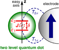
Figure 1: (Color online) Schematic of a two-level magnetic quantum dot coupled to a metallic ferromagnetic electrode. The magnetic moment of the electrode (denoted by a bold arrow) is collinear with the dot’s easy axis. The dot levels have energies $\varepsilon_{1}$ and $\varepsilon_{2}$, respectively, with $\delta$ being the level spacing, while $J$ denotes the exchange interaction. The tunnel matrix elements between the dot and the lead are denoted by $T_{j\sigma}$ for the dot level $j$ and spin $\sigma$.

A bare two-level quantum dot can be characterized by the model Hamiltonian

$$\mathcal{H}_{\textrm{mol}}= \sum_{j=1,2}\sum_{\sigma=\uparrow,\downarrow}\!\!\varepsilon_{j}\,n_{j\sigma}+U\!\!\sum_{j=1,2}\!\!n_{j\uparrow}n_{j\downarrow}+U^{\prime}\!\!\!\!\!\sum_{\sigma,\sigma^{\prime}=\uparrow,\downarrow}\!\!\!\!n_{1\sigma}n_{2\sigma^{\prime}}$$

$$+JS^{2}+DS_{z}^{2}+B_{z}S_{z}.$$ (2)

In the above, $n_{j\sigma}=c_{j\sigma}^{\dagger}c_{j\sigma}$ and $c_{j\sigma}^{\dagger}(c_{j\sigma})$ denotes the creation (annihilation) operator of an electron with spin $\sigma$ and energy $\varepsilon_{j}$ in the $j$th level ($j=1,2$). For convenience, we write the energy levels as $\varepsilon_{1}=\varepsilon-\delta/2$ and $\varepsilon_{2}=\varepsilon+\delta/2$, where $\varepsilon$ is the average value of the two levels while $\delta$ is the level spacing. The Coulomb energy of two electrons of opposite spins occupying the same level is given by $U$ (assumed to be the same for both levels), whereas the inter-level Coulomb correlations are described by $U^{\prime}$. For simplicity, we assume equal correlation energies $U=U^{\prime}$ in the following. Furthermore, $J$ stands for the interlevel exchange interaction with $\bm{S}=\bm{S}_{1}+\bm{S}_{2}$, where $\bm{S}_{j}$ is the electron spin operator for the dot level $j$, $\textbf{S}_{j}=\frac{1}{2}\sum_{\sigma\sigma^{\prime}}c_{j\sigma}^{\dagger}\bm{\sigma}_{\sigma\sigma^{\prime}}c_{j\sigma^{\prime}}$, with $\bm{\sigma}=(\sigma^{x},\sigma^{y},\sigma^{z})$ being the Pauli spin operator. According to the Hund’s rules, this interaction should be generally of a ferromagnetic type $(J<0)$, nonetheless the possibility of a weakly antiferromagnetic coupling has also been reported. Logan et al. (2009) Finally, the lowest order uniaxial magnetic anisotropy is represented by the anisotropy constant $D$, and the last term of Eq. (II.1) describes the Zeeman energy of the dot in an external magnetic field $B_{z}$ applied along the dot’s easy axis, with $g\mu_{\textrm{B}}\equiv 1$.

The Hamiltonian for a ferromagnetic metallic reservoir of noninteracting itinerant electrons is given by

$$\mathcal{H}_{\textrm{lead}}=\sum_{\bm{k}}\sum_{\sigma=\uparrow,\downarrow}\varepsilon_{\bm{k}\sigma}a_{\bm{k}\sigma}^{{\dagger}}a_{\bm{k}\sigma}^{\mbox{}}.$$ (3)

Here, $a_{\bm{k}\sigma}^{{\dagger}}(a_{\bm{k}\sigma}^{\mbox{}})$ creates (annihilates) an electron of energy $\varepsilon_{\bm{k}\sigma}$, where $\bm{k}$ indicates a wave vector, while $\sigma$ is a spin index of the electron. It is important to mention that in the following discussion we assume that magnetic moment of the electrode remains collinear to the dot’s easy axis.

Finally, tunneling of electrons between the electrode and the dot is described in general by

$$\mathcal{H}_{\textrm{tun}}=\sum_{\bm{k}}\sum_{j=1,2}\sum_{\sigma=\uparrow,\downarrow}T_{j\bm{k}\sigma}a_{\bm{k}\sigma}^{{\dagger}}c_{j\sigma}+\textrm{H.c.},$$ (4)

where $T_{j\bm{k}\sigma}$ denotes the tunnel matrix element between the dot’s $j$th level and the electrode, see Fig. 1. In the following we assume that both levels are coupled symmetrically to the electrode, i.e. $T_{1\bm{k}\sigma}=T_{2\bm{k}\sigma}\equiv T_{\bm{k}\sigma}$. Although such foundation is not the most general one, Pustilnik and Glazman (2001); Posazhennikova et al. (2007) it is sufficient for the present analysis of the effects resulting from magnetic anisotropy and exchange field in the context of the underscreened Kondo problem. In order to further facilitate calculations, we assume that the full spin-dependence is included exclusively via the matrix elements $T_{\sigma}$, Choi et al. (2004); Sindel et al. (2007) where the $\bm{k}$-dependence has also been neglected. In addition, we assume a symmetric and flat conduction band extending within the range $[-W,W]$, so that the density of states is $\rho(\omega)\equiv\rho=1/(2W)$, and we use $W\equiv 1$ as the energy unit. Consequently, the spin-dependent hybridization function reads, $\Gamma_{\sigma}=\pi\rho|T_{\sigma}|^{2}$. Now, introducing the spin polarization coefficient $P$ of the electrode, defined as $P=(\Gamma_{\uparrow}-\Gamma_{\downarrow})/(\Gamma_{\uparrow}+\Gamma_{\downarrow})$, the spin-dependent coupling can be parameterized as: $\Gamma_{\uparrow(\downarrow)}=\Gamma(1\pm P)$, with $\Gamma=(\Gamma_{\uparrow}+\Gamma_{\downarrow})/2$.

II.2 Objectives and method of calculations

The main quantity we are interested in is the zero-temperature, spin-dependent equilibrium spectral function of the quantum dot

$$A_{\sigma}^{jj^{\prime}}(\omega)=-\frac{1}{\pi}\Im{\rm m}\langle\!\langle c_{j\sigma}|c_{j^{\prime}\sigma}^{\dagger}\rangle\!\rangle_{\omega}^{\textrm{r}}\ \ \ (j,j^{\prime}=1,2),$$ (5)

with $\langle\!\langle c_{j\sigma}|c_{j^{\prime}\sigma}^{\dagger}\rangle\!\rangle_{\omega}^{\textrm{r}}$ standing for the Fourier transform of the retarded Green’s function $\langle\!\langle c_{j\sigma}|c_{j^{\prime}\sigma}^{\dagger}\rangle\!\rangle_{t}^{\textrm{r}}=-i\theta(t)\langle\{c_{j\sigma}(t),c_{j^{\prime}\sigma}^{\dagger}(0)\}\rangle$. It is worth noting that the spectral function with two identical indices, i.e. $A_{\sigma}^{jj}(\omega)$, is related to the spin-resolved density of states associated with the $j$th level, whereas $A_{\sigma}^{jj^{\prime}}(\omega)$ with $j\neq j^{\prime}$ corresponds to processes of electrons entering and leaving the dot at different levels. Because measuring the spin-resolved components of the spectral function may pose a serious experimental challenge, we will focus on discussing the total spectral function. Thus, we introduce the normalized full spectral function $A(\omega)$,

$$A(\omega)=\pi\sum_{jj^{\prime}}\sum_{\sigma}\Gamma_{\sigma}A_{\sigma}^{jj^{\prime}}(\omega).$$ (6)

The importance of the spectral function $A(\omega)$ stems from the fact that in a two-terminal setup with the second lead being a weakly-coupled probe, e.g. a tip of an STM microscope, the differential conductance of the system at bias voltage $eV$ can be approximated as $\tfrac{\textrm{d}I}{\textrm{d}V}\sim\tfrac{e^{2}}{h}A(\omega=eV)$. Bruus and Flensberg (2004); Csonka et al. (2012) On the other hand, the spectral function for $\omega\to 0$, $A(0)$, determines the linear-response conductance.

In the light of the preceding discussion, the central problem is the calculation of the spectral function $A_{\sigma}^{jj^{\prime}}(\omega)$. In the Kondo regime, this can be reliably done by means of the numerical renormalization group (NRG), Hewson (1997); Wilson (1975); Bulla et al. (2008) which enables us to analyze the static and dynamic properties of the system in the most accurate manner. The essential idea of the method lies in a logarithmic discretization of the conduction band and mapping of the system’s Hamiltonian onto a semi-infinite chain, with the quantum dot residing at the initial site. Iterative diagonalization of the Hamiltonian by adding consecutive sites of the chain allows then for resolving key properties of the system at energy scale $\Lambda^{-n/2}$, with $\Lambda>1$ denoting the discretization parameter and $n$ a given iteration.

In order to address the present problem efficiently, the calculations have been performed with the use of the flexible density-matrix numerical renormalization group (DM-NRG) code. Tóth et al. (2008); Legeza et al. (2008) In this study we exploited the $U_{\textrm{charge}}(1)\times U_{\textrm{spin}}(1)$ symmetries corresponding to conservation of the electron number (charge) and the $z$th component of the total spin.

III Basic concepts

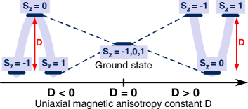
Figure 2: (Color online) Sketch showing how the uniaxial magnetic anisotropy lifts partially the degeneracy between the components of the triplet $S=1$. Note that in reality the energy of the $S_{z}=0$ component is independent of magnetic anisotropy $D$.

III.1 Isolated quantum dot

Before presenting and discussing numerical results on the spectral functions, it is advisable to have a closer look at the energy spectrum of an isolated quantum dot. For the sake of clarity of the following discussion, let us assume that there is no external magnetic field, $B_{z}=0$, so that the system’s behavior is entirely determined by both the sign and magnitude of the uniaxial anisotropy constant $D$, as shown schematically in Fig. 2.

In order to observe the underscreened Kondo effect, the quantum dot needs to be occupied by two electrons which are ferromagnetically exchange-coupled. The ground state of the dot is then a triplet with the components,

$$\left\{\begin{aligned} &|T_{+}\rangle\equiv|S_{z}=+1\rangle=|\!\!\uparrow\rangle_{1}|\!\!\uparrow\rangle_{2},\\ &|T_{0}\rangle\equiv|S_{z}=0\rangle=\frac{1}{\sqrt{2}}\Big{[}|\!\!\uparrow\rangle_{1}|\!\!\downarrow\rangle_{2}+|\!\!\downarrow\rangle_{1}|\!\!\uparrow\rangle_{2}\Big{]},\\ &|T_{-}\rangle\equiv|S_{z}=-1\rangle=|\!\!\downarrow\rangle_{1}|\!\!\downarrow\rangle_{2},\end{aligned}\right.$$ (7)

where $|\chi\rangle_{j}$ denotes the local state of the $j$th level, with $\chi=0,\downarrow,\uparrow,d$ corresponding to zero, spin-down, spin-up and two electrons occupying the level, respectively. As long as an external magnetic field and the magnetic anisotropy are absent, the three triplet states remain degenerate and $\varepsilon_{T_{+}}=\varepsilon_{T_{0}}=\varepsilon_{T_{-}}=2\varepsilon+U+2J$, see Fig. 2. Moreover, the triplet remains the ground state provided the condition, $\delta/2-2U+5J/4<\varepsilon<-\delta/2-U-5J/4$, is satisfied. Weymann and Borda (2010) However, the magnetic anisotropy $D$ lifts this degeneracy and the triplet becomes partially split,

$$\left\{\begin{aligned} &\varepsilon_{T_{+}}\equiv\varepsilon_{T_{1}}=2\varepsilon+U+2J+D,\\ &\varepsilon_{T_{0}}=2\varepsilon+U+2J,\\ &\varepsilon_{T_{-}}\equiv\varepsilon_{T_{1}}=2\varepsilon+U+2J+D.\end{aligned}\right.$$ (8)

As one can see, the energy of states $|T_{+}\rangle$ and $|T_{-}\rangle$ depends on $D$, while the energy of $|T_{0}\rangle$ is independent of $D$. Consequently, when $D<0$, the ground state is two-fold degenerate and corresponds to the states $|T_{+}\rangle$ and $|T_{-}\rangle$, while for $D>0$, the ground state corresponds to $|T_{0}\rangle$, see Fig. 2. This will have a large impact on the Kondo effect, as discussed later on. Note that the presence of magnetic field additionally splits the states $|T_{+}\rangle$ and $|T_{-}\rangle$.

III.2 Effective exchange field and anisotropy

The next question that straightforwardly arises is what happens when the $S=1$ quantum dot becomes attached to a reservoir of electrons. If the temperature is lower than the Kondo temperature, $T<T_{K}$, the conduction electrons can then screen only a half of the dot’s spin, whereas the residual spin-one-half is left unscreened. At zero temperature, the system behaves then as a singular Fermi liquid, i.e. the Fermi liquid with a decoupled $S=\frac{1}{2}$ object. Koller et al. (2005); Mehta et al. (2005) In addition, it turns out that multiple spin-flip processes responsible for the Kondo resonance lead to renormalization of the quantum dot parameters. One can in principle distinguish two different effects associated with such a renormalization. First, the spin degeneracy of the dot is lifted by an effective tunnel-induced exchange field $B_{\textrm{eff}}$. Martinek et al. (2003a, b); Choi et al. (2004); Braun et al. (2004); Martinek et al. (2005); König et al. (2005); Sindel et al. (2007); Weymann (2011); Žitko et al. (2012) It was shown that the exchange field can be tuned by a gate voltage Hauptmann et al. (2008) and can be compensated by applying an external magnetic field. Pasupathy et al. (2004); Weymann and Borda (2010); Hauptmann et al. (2008); Gaass et al. (2011) The second effect, on the other hand, is related to the renormalization of the anisotropy constant, $\Delta D$, which results in an effective anisotropy $D_{\rm eff}$, $D_{\rm eff}=D+\Delta D$, as shown schematically in Figs. 3(a)-(c). This renormalization is independent of the spin polarization $P$ of the lead, while it depends weakly on the gate voltage and cannot be compensated by external magnetic field.

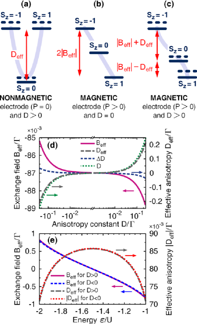
Figure 3: (Color online) (a)–(c) Schematic representing level renormalization due to the effective anisotropy constant $D_{\rm eff}$ and effective exchange field $B_{\rm eff}$ for the quantum dot with $S=1$. Dashed lines in (a) and (c) correspond to energy levels without the renormalization of the uniaxial magnetic anisotropy constant, $D_{\rm eff}=D$, see Eq. (11). It is assumed that $B_{\rm eff}<0$, so that the ground state (in (b) and (c)) is $|T_{+}\rangle$. Bottom panel: the dependence of $B_{\rm eff}$ and $D_{\rm eff}$ on the anisotropy constant $D$ for $\varepsilon/U=-1.4$ (d) and on the level position $\varepsilon$ in the Coulomb blockade regime for $|D|/\Gamma=0.1$ (e). Note that in (e) for $D<0$ one also gets $D_{\rm eff}<0$, but for practical reasons $|D_{\rm eff}|$ is plotted. For comparison, in (d) we also show $\Delta D$ and $D$. The other parameters are: $\varepsilon=-17.5\Gamma$, $\delta=2.5\Gamma$, $U=12.5\Gamma$, $J=-2.5\Gamma$, and $P=0.5$.

The renormalized energies $\widetilde{\varepsilon}_{T_{i}}$ ($i=0,\pm$) of the triplet state can be found from the second-order perturbation theory in the tunneling Hamiltonian as $\widetilde{\varepsilon}_{T_{i}}=\varepsilon_{T_{i}}+\delta\varepsilon_{T_{i}}$ ($i=0,\pm$), where $\delta\varepsilon_{T_{i}}$ is the second-order correction of the respective triplet component. The renormalized triplet energies may be written in the following way

$$\left\{\begin{aligned} &\widetilde{\varepsilon}_{T_{+}}=\varepsilon_{T_{0}}+\delta\varepsilon_{T_{0}}+D_{\rm eff}+B_{\rm eff}+B_{z},\\ &\widetilde{\varepsilon}_{T_{0}}=\varepsilon_{T_{0}}+\delta\varepsilon_{T_{0}},\\ &\widetilde{\varepsilon}_{T_{-}}=\varepsilon_{T_{0}}+\delta\varepsilon_{T_{0}}+D_{\rm eff}-B_{\rm eff}-B_{z},\end{aligned}\right.$$ (9)

where the effective exchange field $B_{\textrm{eff}}$ induced by a ferromagnetic contact is given by Martinek et al. (2005)

$$B_{\textrm{eff}}=-\frac{\Gamma P}{\pi}\!\sum_{j=\pm}\!\int^{\prime}\!\!\!\textrm{d}\omega\,\Bigg{\{}\frac{1-f(\omega)}{\omega-E_{T_{1},1j}}+\frac{f(\omega)}{\omega+E_{T_{1},3j}}\Bigg{\}},$$ (10)

and the effective anisotropy $D_{\textrm{eff}}$ can be expressed as

$$D_{\textrm{eff}}=D+\Delta D$$ (11)

with the renormalization of the anisotropy constant $\Delta D$ of the form

$$\Delta D=\frac{\Gamma}{\pi}\!\sum_{j=\pm}\!\int^{\prime}\!\!\!\textrm{d}\omega\,\Bigg{\{} \frac{1-f(\omega)}{\omega-E_{T_{0},1j}}-\frac{1-f(\omega)}{\omega-E_{T_{1},1j}}$$

$$-\Bigg{[} \frac{f(\omega)}{\omega+E_{T_{0},3j}}-\frac{f(\omega)}{\omega+E_{T_{1},3j}}\Bigg{]}\Bigg{\}}.$$ (12)

The prime superscript in the above equations symbolizes Cauchy’s principal value integrals, and $f(\omega)$ stands for the Fermi-Dirac distribution function of the contact. We note that terms involving $1-f(\omega)$ represent here electron-like charge fluctuations, due to which the molecule loses one electron, while terms with $f(\omega)$ refer to the hole-like processes, when the charge of the molecule is increased by one electron. Furthermore, $E_{\alpha,\beta}=\varepsilon_{\alpha}-\varepsilon_{\beta}$ is the energy difference between the corresponding states. The respective energies of singly occupied states are, $\varepsilon_{1\pm}=\varepsilon\pm\delta/2+3J/4+D/4$, while the energies of states with three electrons are given by, $\varepsilon_{3\pm}=3\varepsilon+3U\pm\delta/2+3J/4+D/4$. In Eq. (9) $\delta\varepsilon_{T_{0}}$ ($\delta\varepsilon_{T_{0}}<0$) denotes the second-order energy correction of the triplet component $|T_{0}\rangle$ (uniform shift of the whole triplet). The explicit form of $\delta\varepsilon_{T_{0}}$ is not relevant for the present discussion, since it is the difference between the above energies of triplet components that determines the occurrence and features of the Kondo effect. In the low temperature regime, which except Sec. IV.3 is in the main scope of the work, Eqs. (10) and (III.2) simplify significantly,

$$B_{\rm eff}=\frac{P\Gamma}{\pi}\ln\left|\frac{E_{T_{1},1-}}{E_{T_{1},3-}}\cdot\frac{E_{T_{1},1+}}{E_{T_{1},3+}}\right|,$$ (13)

$$\Delta D=\frac{\Gamma}{\pi}\ln\left|\frac{E_{T_{1},1-}}{E_{T_{0},1-}}\cdot\frac{E_{T_{1},1+}}{E_{T_{0},1+}}\cdot\frac{E_{T_{1},3-}}{E_{T_{0},3-}}\cdot\frac{E_{T_{1},3+}}{E_{T_{0},3+}}\right|.$$ (14)

We also note that the energies of triplet, Eq. (9), explicitly include the external magnetic field $B_{z}$. This will be relevant for the discussion of system transport properties in the presence of magnetic field, that will be presented in the next section.

From Eqs. (10) and (13) follows that the exchange field is an intrinsic effect resulting from the spin-dependence of tunneling processes, and vanishes for $P\to 0$. Moreover, $B_{\rm eff}$ displays monotonic dependence on the level position $\varepsilon$: with $B_{\rm eff}=0$ at the particle-hole symmetry point of the model, i.e. for $\varepsilon=-3U/2$, and $B_{\rm eff}\lessgtr 0$ for $\varepsilon\gtrless-3U/2$. This is shown in Fig. 3(e). In addition, $B_{\rm eff}$ also depends on the anisotropy constant $D$, see Fig. 3(d). This dependence, however, is much weaker than the dependence on $\varepsilon$.

On the other hand, since $\varepsilon_{T_{1}}=\varepsilon_{T_{0}}+D$, one can immediately conclude from Eqs. (III.2) and (14) that $\Delta D\to 0$ as $D\to 0$. It is interesting to note that tunneling of electrons leads to suppression of the magnetic anisotropy, $\Delta D\lessgtr 0$ for $D\gtrless 0$, in the whole Coulomb blockade regime. Furthermore, unlike the effective exchange field, $\Delta D$ is an even function of the level position $\varepsilon$ with the extremum (maximum for $D>0$ and minimum for $D<0$) in the particle-hole symmetry point, where

$$\Delta D_{\varepsilon=-\frac{3U}{2}}=\frac{\Gamma}{\pi}\ln\left|\frac{(2U-5J-3D)^{2}-4\delta^{2}}{(2U-5J+D)^{2}-4\delta^{2}}\right|.$$ (15)

The dependence of the effective anisotropy $D_{\rm eff}$ on the magnetic anisotropy constant as well as on the level position is shown in Fig. 3(d,e). One can note that $D_{\rm eff}$ depends strongly on $D$ and only weakly on the level position, which is just opposite to the behavior of the exchange field $B_{\rm eff}$. Moreover, while $B_{\rm eff}$ is due to the spin-dependence of tunneling processes and vanishes for nonmagnetic leads, $D_{\rm eff}$ does not depend on the spin polarization and is finite also when $P=0$ – as long as $D\neq 0$.

The above discussion suggests that transport properties should be mainly determined by the interplay of the effective anisotropy $D_{\rm eff}$, contact-induced exchange field $B_{\rm eff}$ and the Kondo temperature $T_{K}$. Additionally, the behavior of the total spectral function also significantly depends on the tunnel-coupling strength $\Gamma$ (to observe the Kondo physics the coupling should be sufficiently large). Experimental results show that the Kondo phenomena in quantum dots can be observed when $\Gamma$ is of the order of a few tenths of meV for temperatures of the order of mK.  Goldhaber-Gordon et al. (1998); Simmel et al. (1999); Sasaki et al. (2000); Kogan et al. (2003) Accordingly, in numerical calculations we assume $\Gamma=0.5$ meV and use $\Gamma$ as the relevant energy scale. For the quantum dot we assume the parameters that are comparable to those observed in experiments, $\varepsilon=-17.5\Gamma$ ($\varepsilon=-8.75$ meV), $\delta=2.5\Gamma$ ($\delta=1.25$ meV), $U=12.5\Gamma$ ($U=6.25$ meV), and $J=-2.5\Gamma$ ($J=-1.25$ meV), if not stated otherwise. Note that we assumed $\varepsilon/U>-3U/2$, so that if the lead is ferromagnetic, the ground state is $|T_{+}\rangle$ due to $B_{\rm eff}<0$, see also Fig. 3(c).

IV Numerical results and discussion

In the following we present and discuss numerical results on the dot’s spectral density as a function of the anisotropy constant $D$, spin polarization of the lead $P$, and external magnetic field $B_{z}$. The main focus, however, will be on the effects arising from the magnetic anisotropy and effective exchange field. Generally, the magnetic anisotropy in systems under consideration can take fairly large values, and can range approximately from $|D|\lesssim 0.05$ meV for single-molecule magnets,  Gatteschi et al. (2006); Heersche et al. (2006); Zyazin et al. (2010); Mannini et al. (2010) up to a few meV for magnetic adatoms like Mn, Fe, Co,  Hirjibehedin et al. (2007); Otte et al. (2008); Brune and Gambardella (2009) or some magnetic molecules. Parks et al. (2010) Furthermore, Park et al. Parks et al. (2010) have shown that mechanical strain in a certain type of Co complexes allows for a fully controllable and continuous change of the magnetic anisotropy of a molecule. This effect occurs since the stretching or squeezing of a molecule leads to modification of the crystal field exerted on the central Co ion. For the above reasons, the following results will be presented for a wide range of both positive and negative uniaxial anisotropy constant $D$.

IV.1 Influence of uniaxial magnetic anisotropy

Figure 4: (Color online) Total normalized spectral function $A(\omega)$ of the dot for $\omega\rightarrow 0$, $A(0)$, as a function of the uniaxial magnetic anisotropy constant $D$ for several values of the interlevel exchange interaction $J$ in the presence of (a) nonmagnetic (NM) and (b) ferromagnetic (FM) electrode. The insets in (a) and (b) display $A(0)$ as a function of $D/\Gamma$ plotted in a linear scale in the case of nonmagnetic (a) and ferromagnetic (b) electrode for different values of $J$. Note that in the inset in (a) the Kondo peaks have been shifted by $-0.01$ for better visibility. (c) Variation of the spectral function with the energy $\omega$ and uniaxial magnetic anisotropy constant $D$ for $J/\Gamma=-2.5$. (d) Cross-sections of the plot in (c) for selected values of the uniaxial anisotropy constant $D>0$. The other parameters are: $\varepsilon=-17.5\Gamma$, $\delta=2.5\Gamma$, $U=12.5\Gamma$, and $P=0.5$ (except (a) where $P=0$).

IV.1.1 Nonmagnetic lead

To begin with, let us first discuss briefly how the spectral function of the system depends on the magnetic anisotropy in the case of a nonmagnetic electrode. Cornaglia et al. (2011) Figure 4(a) shows the dependence of $A(0)$ on $D$ for several values of the exchange interaction $J$. It can be seen that $A(0)\approx 2$ for $|D|<T_{K}$, where $T_{K}$ is the Kondo temperature, with $A(0)$ decreasing below its unitary value once $|D|\gtrsim T_{K}$. Moreover, the resonance dies away more abruptly for $D>0$, where the spectral function is practically equal to zero above some threshold value of the anisotropy constant. Accordingly, one should expect there a vanishingly small linear conductance of the system. Indeed, such a behavior has been observed by Parks et al., Parks et al. (2010) who reported splitting of the Kondo peak due to stretching the molecule. The asymmetry between the decrease of $A(0)$ for positive and negative $D$ is associated with different ground states of the quantum dot, see Fig. 2. For $D>0$ and $D_{\rm eff}\gtrsim T_{K}$, the ground state is $|T_{0}\rangle$ and no spin-flip processes are possible, consequently $A(0)$ becomes abruptly suppressed. On the other hand, for $D<0$ and $|D_{\rm eff}|\gtrsim T_{K}$, the ground state is two-fold degenerate, with equally occupied states $|T_{+}\rangle$ and $|T_{-}\rangle$, see Eq. (9). Due to the spin selection rules for tunneling processes, the second-order spin-flip cotunneling is then suppressed and the Kondo resonance becomes suppressed as well [$A(0)$ starts decreasing]. However, there are fourth-order tunneling processes that are still possible and therefore $A(0)$ decreases rather slowly with increasing $|D|$, opposite to the case of positive $D$.

The features discussed above depend on the Kondo temperature $T_{K}$. Since $T_{K}$ is a function of the energy difference between the ground state and single and three-particle virtual states, the Kondo temperature can be tuned by changing the exchange interaction $J$. When increasing $|J|$, one effectively increases the energy differences and $T_{K}$ becomes decreased. Accordingly, the suppression of the Kondo effect occurs for smaller values of $D$. This can be clearly seen in Fig. 4(a). Note that the width of the maximum in $A(0)$ as a function of $D$ is roughly equal to $2T_{K}$.

IV.1.2 Ferromagnetic lead

The situation becomes much more interesting when the nonmagnetic reservoir is replaced by the ferromagnetic one. The dependence of the spectral function $A(0)$ on $D$ is presented in Fig. 4(b). First, for small values of $|D|$, and thus also $|D_{\rm eff}|$, the height of the Kondo resonance is significantly reduced as compared to the case of a nonmagnetic electrode, which is due to the presence of exchange field $B_{\rm eff}$. Second, as $D>0$ increases, one observes the revival of the Kondo effect at some resonant value of the magnetic anisotropy constant, $D=D_{\textrm{res}}$. However, further increase in $D$ results in the drop of the spectral function to zero, so that the behavior of the system for large and positive $D$ resembles that of a dot coupled to a nonmagnetic electrode. In addition, the dependence on the exchange coupling is also qualitatively similar to that in the nonmagnetic case. When increasing $|J|$, $T_{K}$ is reduced and the width of the Kondo resonance as a function of $D$ becomes decreased as well, see the inset in Fig. 4(b). In fact, the width of the Kondo resonance for a given value of $J$ is of the same order in the case of nonmagnetic and ferromagnetic leads, compare the insets in Figs. 4(a,b). In addition, the value of $D_{\rm res}$ decreases with increasing $J$, which is due to the corresponding dependence of $B_{\rm eff}$ and $D_{\rm eff}$ on the exchange coupling $J$.

Since the spectral function can be substantially modified upon altering the anisotropy constant $D$, the following discussion will be focused on the interplay of $D_{\rm eff}$ and $B_{\rm eff}$, that governs the transport behavior in the Kondo regime. In the remaining part of the paper we will present and discuss numerical results for a fixed value of the exchange coupling, $J/\Gamma=-2.5$ [corresponding to the bold lines in Figs. 4(a,b)].

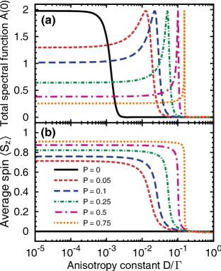
Figure 5: (Color online) (a) Total normalized spectral function $A(\omega)$ of the dot for $\omega\rightarrow 0$ and (b) the corresponding expectation value of the dot’s spin $z$th component as functions of the uniaxial magnetic anisotropy constant $D$. Except $J/\Gamma=-2.5$, remaining parameters are the same as in Fig. 4.

As follows from Eq. (13), the strength of $B_{\textrm{eff}}$ depends on the spin polarization $P$ of the reservoir, $B_{\textrm{eff}}\sim P\Gamma$. Moreover, through the energy differences between respective states, $B_{\textrm{eff}}$ is a function of all parameters of the model, including the magnetic anisotropy constant $D$. First of all, unlike $\Delta D$ [see Eq. (14)], $B_{\textrm{eff}}$ is finite for $D\rightarrow 0$. More specifically, for parameters used in Figs. 3(d) and 4(c,d) it approaches a constant value of $B_{\textrm{eff}}/\Gamma\approx-0.087$. Since the exchange field lowers the energy of the highest-weight triplet component $|T_{+}\rangle$, see schema (b) in Fig. 3, one can observe almost full spin polarization of the dot, $\langle S_{z}\rangle\to 1$, see Fig. 5(b) for $D\to 0$. Note, however, that the dot’s spin can be flipped to $\langle S_{z}\rangle\to-1$ for $\varepsilon<-3U/2$, where $B_{\rm eff}>0$ and $|T_{-}\rangle$ becomes the ground state of the system. This can be achieved for instance by applying a gate voltage. In addition, $B_{\rm eff}$ also depends on the anisotropy constant and it can either increase or decrease depending on the sign of $D$, see the solid line in Fig. 3(d). For the parameters used in calculations, the modification of $B_{\rm eff}$ for $|D|=\Gamma/10$ is however rather small ($\sim 1\%$). The variation of the exchange field as a function of $D$ is thus of rather minor significance for $\Gamma\gg|D|$, but nevertheless the interplay of $D$ ($D_{\rm eff}$) and $B_{\textrm{eff}}$ turns out to be crucial for the occurrence of the Kondo effect.

Let us focus first on the case of $D<0$, where no restoration of the Kondo resonance takes place, see the left side of Fig. 4(b). The ground state for $P=0$ would be doubly degenerate. Because of the exchange field, this degeneracy, however, is lifted and the ground state is $|T_{+}\rangle$. The state $|T_{+}\rangle$ remains the ground state in the whole range of $D<0$ considered in this paper. In consequence, there is no Kondo effect for $D<0$.

The situation, however, is much more complex in the case of $D>0$, where the restoration of the Kondo resonance appears, see the right side of Fig. 4(b). For small values of $D$, where the dominant energy scale due to renormalization processes is set by the exchange field $B_{\textrm{eff}}$, the ground state is $|T_{+}\rangle$ and the situation is similar to that for $D<0$. Nonetheless, as the magnetic anisotropy grows, the condition $B_{\textrm{eff}}+D_{\textrm{eff}}=0$ becomes satisfied at some point (note that for the assumed parameters $B_{\rm eff}<0$ while $D_{\rm eff}>0$) and the state $|T_{+}\rangle$ gets degenerate with the state $|T_{0}\rangle$. The difference between the spin $z$th components of the states $|T_{+}\rangle$ and $|T_{0}\rangle$ is 1, so the second-order spin-flip cotunneling processes are possible and the Kondo effect can be restored. $A(0)$ reaches then its maximal value.

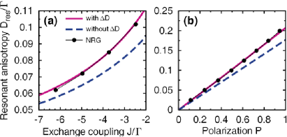
Figure 6: (Color online) (a) Dependence of the magnetic anisotropy constant $D_{\textrm{res}}$ at which the Kondo resonance is restored on the interlevel exchange coupling $J$ for $P=0.5$ and (b) on the spin polarization $P$ for $J/\Gamma=-2.5$. Other parameters as in Fig. 4.

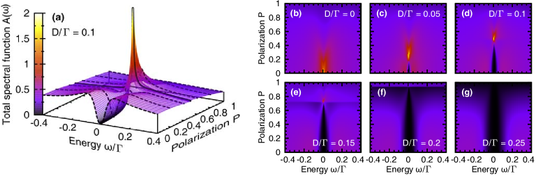
Figure 7: (Color online) Total normalized spectral function $A(\omega)$ of the dot shown as a function of energy $\omega$ and the spin polarization parameter $P$ for indicated values of the uniaxial magnetic anisotropy constant $D$. Other parameters are the same as in Fig. 5.

The above described behavior can be also observed in the full energy dependence of the spectral function $A(\omega)$, see Figs. 4(c,d). The Kondo resonance is restored when $D=D_{\rm res}\approx\Gamma/10$ and is immediately suppressed once $D>D_{\rm res}$. On the other hand, the suppression is less effective on the left side of the restored Kondo resonance, as already discussed above. In addition, the energy dependence of the spectral function in Fig. 4(d) reveals small side peaks for $D>D_{\rm res}$, which are reminiscent of the Kondo effect and occur for energies $\omega\approx\pm|D_{\rm eff}+B_{\rm eff}|$ corresponding to restored degeneracy of the states $|T_{+}\rangle$ and $|T_{0}\rangle$. Apart from this, at large energies, $\omega\approx\pm U$, there are typical Hubbard resonance peaks.

Since the occurrence of the Kondo resonance depends on the ratio of $B_{\rm eff}$ and $D_{\rm eff}$, it is interesting to study variation of $A(0)$ with $D$ for different values of lead’s spin polarization. This is shown in Fig. 5(a). When $P=0$, $A(0)$ shows a maximum for such $D$ that the condition $|D_{\rm eff}|\lesssim T_{K}$ is fulfilled. If the spin polarization is finite, the maximum is shifted towards larger values of anisotropy and occurs precisely when the states $|T_{+}\rangle$ and $|T_{0}\rangle$ become degenerate, i.e. for $D=D_{\rm res}$. Note, that the width of the peak in $A(0)$ as a function of $D$ is of the same order for all values of spin polarization $P$. Since the dot is coupled to one electron reservoir, only half of the dot’s spin can be screened by the conduction electrons for $D=D_{\rm res}$. As a result, in the underscreened Kondo regime the expectation value of the dot’s spin should reach $\langle S_{z}\rangle\approx 1/2$, since the unscreened residual spin-1/2 is polarized due to the presence of exchange field. This can be seen in Fig. 5(b), which shows the dependence of $\langle S_{z}\rangle$ on $D$ for several values of $P$. For $D<D_{\rm res}$, the ground state of the dot is $|T_{+}\rangle$ and $\langle S_{z}\rangle$ is close to one, while for $D>D_{\rm res}$, the ground state is $|T_{0}\rangle$ and $\langle S_{z}\rangle=0$. On the other hand, for $D\approx D_{\rm res}$, one finds $\langle S_{z}\rangle=1/2$, see Fig. 5(b). However, closer analysis of $\langle S_{z}\rangle$ shows that it actually fails in attaining its maximum value for $D<D_{\textrm{res}}$. This is related with the fact that the ratio $U/\Gamma$ is relatively large for the assumed parameters and there is nonzero occupation probability of other spin components of the triplet. Weymann and Borda (2010) However, when increasing the spin polarization $P$ of the lead, the splitting of the levels grows due to the exchange field, $B_{\rm eff}\sim P\Gamma$, and the occupation of the triplet component $|T_{+}\rangle$ is raised. In consequence, one finds that $\langle S_{z}\rangle\to 1$, if $P\to 1$.

Knowing the analytical condition, $B_{\textrm{eff}}+D_{\textrm{eff}}=0$, for the occurrence of the Kondo resonance for $D>0$, it is instructive to analyze the role of magnetic anisotropy renormalization. For this purpose, in Fig. 6 we present the dependence of $D_{\textrm{res}}$ on $J$ and $P$. The solid (dashed) line corresponds to $D_{\textrm{res}}$ determined from the analytical formulas for $B_{\textrm{eff}}$ and $D_{\textrm{eff}}$ with (without) including $\Delta D$, while the dots show $D_{\textrm{res}}$ obtained from NRG data. As one can see, the NRG results are in very good agreement with analytical results when $\Delta D$ is taken into account. Thus, the estimations based on the analytical expressions for the exchange field and effective anisotropy, Eqs. (13)-(14), are quite satisfactory. The renormalization of $D$ is thus an important effect that needs to be included in theoretical considerations of spin $S\gtrsim 1$ systems exhibiting magnetic anisotropy.

To demonstrate additional features of the interplay between magnetic anisotropy and exchange field, we show in Fig. 7 the energy and spin polarization dependence of the normalized spectral function $A(\omega)$. The full energy dependence of the spectral function may prove to be useful in predicting some qualitative information concerning transport properties of the system at a finite bias. As it was discussed earlier, the spin polarization $P$ determines the strength of $B_{\textrm{eff}}$, without affecting $D_{\rm eff}$. In consequence, all $\omega$-dependent features in Fig. 7 should in principle stem from the changes of $B_{\textrm{eff}}$ with respect to $D_{\textrm{eff}}$. For $P<P_{\textrm{res}}$, where $P_{\rm res}$ is the value of spin polarization at which the Kondo resonance is restored, one observes a well-pronounced dip, which indicates that the system’s ground state is nonmagnetic, i.e. $|T_{0}\rangle$. In the present picture, increasing $\omega$ turns to be equivalent (to some extent) to the application of an external bias voltage when the dot would be asymmetrically attached to two contacts. Csonka et al. (2012) For $P\rightarrow 0$, the spectral function attains then its local maximum at $\omega$ that approximately corresponds to the degeneracy of the states $|T_{0}\rangle$ and $|T_{+}\rangle$. From this, in turn, $D_{\textrm{eff}}$ can be straightforwardly obtained, i.e. $D_{\textrm{eff}}\approx\omega$. As $P$ increases, the magnitude of the exchange field $|B_{\textrm{eff}}|$ increases as well, and this is accompanied by a decrease in the energy gap $B_{\textrm{eff}}+D_{\textrm{eff}}$. This appears then as a gradual narrowing of the dip, until the two states, i.e. $|T_{+}\rangle$ and $|T_{0}\rangle$, become degenerate, and the Kondo resonance is restored, see Figs. 7(a)-(e). For larger values of $P$, the system’s ground state is $|T_{+}\rangle$ and the Kondo resonance is suppressed again. There are however two satellite peaks at energies $\omega\approx\pm|D_{\rm eff}+B_{\rm eff}|$, whose position depends linearly on $P$, and whose height diminishes as $P$ grows further. Moreover, it turns out that for larger values of $D$, see Figs. 7(f)-(g), no restoration of the Kondo effect is possible. This is because the magnitude of exchange field is too low to compensate the effective anisotropy $D_{\rm eff}$ and the degeneracy of states cannot be restored even if $P\to 1$.

IV.2 Influence of an external magnetic field

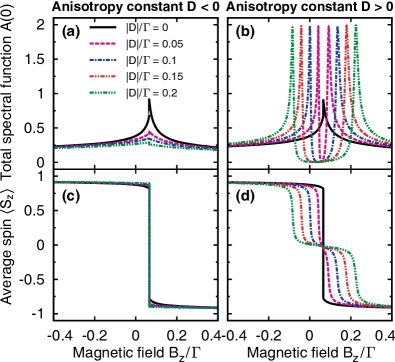
Figure 8: (Color online) Dependence of the total normalized spectral function $A(\omega)$ for $\omega\rightarrow 0$ (a,b) and the average $z$th component of the spin $\langle S_{z}\rangle$ (c,d) on an external magnetic field $B_{z}$ oriented along the dot’s easy axis. Different lines correspond to selected values of the uniaxial magnetic anisotropy constant $D$, and the left panel corresponds to $D<0$, while the right panel refers to $D>0$. Except for $P=0.5$ and $J/\Gamma=-2.5$, all remaining parameters are the same as in Fig. 4.

Figure 8 shows the dependence of the spectral function $A(0)$ and the average value of dot’s spin $\langle S_{z}\rangle$ on the magnetic field $B_{z}$. It can be noticed that while the Kondo effect for $D<0$ can be restored just for a single value of $B_{z}$, for $D>0$ the restoration occurs twice. In order to understand this behavior one should bear in mind that the external magnetic field affects the components $|T_{+}\rangle$ and $|T_{-}\rangle$ of the triplet state and thus can be used to compensate the splitting induced by exchange field $B_{\rm eff}$ due to ferromagnetic contact, Weymann and Borda (2010) see Eq. (9). In the case of vanishing $D$ and $B_{z}=0$, the Kondo resonance is suppressed due to the exchange field $B_{\rm eff}$ and the system ground state is $|T_{+}\rangle$. With increasing $B_{z}$, all the three components of the triplet state become degenerate once $B_{\rm eff}+B_{z}\approx 0$, and the system is in the underscreened Kondo regime. Nevertheless, because only a half of the dot’s spin can be screened by conduction electrons, the remaining spin-$1/2$ can be polarized by any infinitesimal magnetic field (at zero temperature). This leads to strong sensitivity of the ground state on magnetic field, which hinders the full restoration of the underscreened Kondo effect. Weymann and Borda (2010)

For $D<0$, the increase of $B_{z}$ can only restore the degeneracy between the highest and lowest-weight components of the triplet. In consequence, one observes a small peak at $B_{z}\approx|B_{\rm eff}|$, see Fig. 8(a), where the ground state changes from $|T_{+}\rangle$ to $|T_{-}\rangle$, see Fig. 8(c). Note that the position of this peak does not depend on $D$. On the other hand, for positive anisotropy $D>0$, the full restoration of the Kondo effect is possible, see Fig. 8(b). Moreover, contrary to single-level quantum dots, Gaass et al. (2011) the restoration with increasing $B_{z}$ occurs twice. This can be understood by studying the evolution of the ground state with magnetic field, see Fig. 8(d). For $B_{z}=0$ and $D>0$, the ground state is a singlet, $|T_{0}\rangle$. By lowering the magnetic field, $B_{z}<0$, the ground state changes to $|T_{+}\rangle$ for $B_{z}\approx-D_{\rm eff}-B_{\rm eff}$, while by increasing $B_{z}$, once $B_{z}\approx D_{\rm eff}-B_{\rm eff}$, the ground state changes to $|T_{-}\rangle$. Consequently, once $B_{z}\approx\pm D_{\rm eff}-B_{\rm eff}$, the two-fold degeneracy of the ground state becomes restored and the Kondo effect can develop. One observes then two maxima in $A(0)$, see Fig. 8(b). Note, however, that different states are responsible for these two Kondo peaks. For $B_{z}\approx-D_{\rm eff}-B_{\rm eff}$, it is the degeneracy between the states $|T_{+}\rangle$ and $|T_{0}\rangle$ that results in the formation of the Kondo effect, while for $B_{z}\approx D_{\rm eff}-B_{\rm eff}$, the states $|T_{-}\rangle$ and $|T_{0}\rangle$ are degenerate. It is also worth noting that since the Kondo temperature is rather independent of $D$, the width of the restored Kondo peaks is the same for all values of $D$, see Fig. 8(b).

From the magnetic field dependence of $A(0)$ one can obtain the information about the magnitude of both $B_{\rm eff}$ and $D_{\rm eff}$. Suppose the restoration of the Kondo effect occurs for $B_{z}=B_{\rm res}^{(1)}$ and $B_{z}=B_{\rm res}^{(2)}$, then the effective anisotropy constant can be related to a half of the distance between the two restored Kondo resonances $D_{\rm eff}=|B_{\rm res}^{(1)}-B_{\rm res}^{(2)}|/2$. On the other hand, the magnitude of the exchange field can be found from the average, $B_{\rm eff}=-(B_{\rm res}^{(1)}+B_{\rm res}^{(2)})/2$. Studying the magnetic field dependence of the zero-energy spectral function, which would correspond to measuring the low-temperature zero-bias conductance, may be thus useful in obtaining information about both the effective anisotropy and exchange field.

IV.3 Temperature dependence of linear conductance

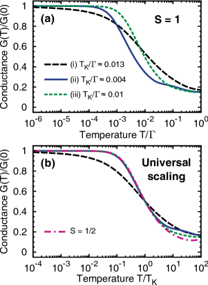
Figure 9: (Color online) The temperature dependence of the normalized linear conductance $G(T)/G(0)$ (a) and the universal scaling curves (b). The relevant curves correspond to (i) underscreened Kondo effect, with $D=0$, $P=0$, $B_{z}=0$, (ii) restored Kondo resonance when $B_{\rm eff}+D_{\rm eff}=0$, with $D/\Gamma\approx 0.1$, $P=0.5$, $B_{z}=0$, and (iii) restored Kondo resonance by magnetic field $B_{z}=D_{\rm eff}-B_{\rm eff}$, with $D/\Gamma\approx 0.2$, $P=0.5$, $B_{z}/\Gamma\approx 0.22$. The curves (ii) and (iii) display scaling typical for spin $S=1/2$ Kondo effect [dotted-dashed line in (b)]. Other parameters the same as in Fig. 4 with $J/\Gamma=-2.5$.

It is very instructive to study the temperature $T$ dependence of the linear conductance, $G(T)$, in the underscreened Kondo regime and for parameters where the restoration of the Kondo effect appears. Generally, the conductance in the underscreened Kondo regime can be measured by attaching a second weakly-coupled electrode, which due to much smaller Kondo temperature, is irrelevant for screening the dot’s spin. Roch et al. (2009); Parks et al. (2010) The linear conductance has been calculated by means of NRG method with the full density-matrix, and the Meir-Wingreen formula. Meir and Wingreen (1992) The normalized linear conductance as a function of temperature $T$ is shown in Fig. 9(a) for the underscreened Kondo effect (dashed line), i.e. for $P=D=B_{z}=0$, and for parameters where the restoration of the Kondo effect occurs – first when the condition $D_{\rm eff}+B_{\rm eff}=0$ is met (solid line) and second when the restoration is obtained by applying magnetic field, i.e. when $D_{\rm eff}-B_{\rm eff}-B_{z}=0$ is satisfied (dotted line). The relevant Kondo temperatures are also given in the figure. $T_{K}$ is defined here as the value of $T$ where $G(T)/G(0)=1/2$. Figure 9(b) displays the universal scaling curves of normalized conductance $G(T)/G(0)$ as a function of $T/T_{K}$. For $D=0$, $P=0$ and in the absence of magnetic field, we observe scaling typical for the underscreened Kondo regime, Posazhennikova and Coleman (2005) which has been recently measured experimentally. Roch et al. (2009) The temperature dependence of the linear conductance for parameters where the restoration of the Kondo effect occurs also turns out to be universal, see Fig. 9(b), however the scaling is completely different from the underscreened Kondo effect. For parameters where the restoration occurs, the ground state is two-fold degenerate, i.e. either $|T_{+}\rangle$ and $|T_{0}\rangle$ or $|T_{0}\rangle$ and $|T_{-}\rangle$ components of the triplet state are degenerate, therefore one should expect the same scaling as for the spin $S=1/2$ Kondo effect.  Kretinin et al. (2011) Indeed, we compare the universal scaling of the linear conductance for restored Kondo resonances of $S=1$ quantum dot with the scaling for typical $S=1/2$ Kondo effect and find perfect agreement, see Fig. 9(b).

V Summary and conclusions

By means of numerical renormalization group method, we have studied transport properties of a magnetic $S=1$ quantum dot coupled to a ferromagnetic lead in the underscreened Kondo regime. Due to the coupling of the dot to an external lead, the following two effective parameters are shown to play important role: the effective exchange field $B_{\rm eff}$ and the effective anisotropy constant $D_{\rm eff}$. The interplay of the corresponding interactions is crucial to understand behavior of the system transport properties, especially regarding the evolution (suppression or restoration) of the Kondo effect as a function of various parameters of the model considered. Using the second-order perturbation theory, we have derived analytical formulas for both $B_{\rm eff}$ and $D_{\rm eff}$. It turns out that the effective anisotropy $D_{\rm eff}$ depends strongly on $D$ and $D_{\rm eff}\to 0$ as $D\to 0$. Furthermore, $D_{\rm eff}$ is an even and weakly changing function of the level position $\varepsilon$, with an extremum at the particle-hole symmetry point, $\varepsilon=-3U/2$, and does not depend on the spin polarization of the ferromagnetic lead. The effective exchange field $B_{\rm eff}$, on the other hand, depends linearly on lead’s spin polarization $P$ and $B_{\rm eff}\to 0$ for $P\to 0$. Furthermore, it is an odd function of level position $\varepsilon$ and vanishes at the particle-hole symmetry point, $\varepsilon=-3U/2$. $B_{\rm eff}$ also depends on $D$, although this dependence is rather weak. We compared the analytical formulas for $B_{\rm eff}$ and $D_{\rm eff}$ with the NRG data and found very good agreement.

By performing extensive NRG calculations, we have studied variation of the spectral functions with various parameters of the system. We have shown that the underscreened Kondo effect is generally suppressed due to the presence of magnetic anisotropy and exchange field. It can be, however, restored by tuning the magnetic anisotropy constant $D$. The restoration occurs only for positive anisotropy, $D>0$, while no restoration takes place when the magnetic anisotropy is negative, $D<0$. Moreover, the restoration of the Kondo resonance also occurs as a function of magnetic field applied along the easy axis. By sweeping the magnetic field, the Kondo effect can be restored twice in a single sweep. The restoration always occurs due to the degeneracy between the components of the triplet state that differ in the spin $S_{z}$ quantum number by $1$.

We have also determined the temperature dependence of the linear conductance for some characteristic parameters, where the restoration of the Kondo effect occurs. It turned out that the restored Kondo resonances exhibit a universal scaling as a function of $T/T_{K}$ characteristic of spin $S=1/2$ Kondo quantum dots. This is due to the fact that for parameters where the restoration of the Kondo effect is possible, the ground state is two-fold degenerate.

Finally, we would like to emphasize that when considering spin-resolved transport through nanostructures of spin $S\geq 1$ exhibiting magnetic anisotropy, there are two relevant and distinct effects that need to be taken into account in order to fully understand behavior of the system. The first one is the exchange field induced by ferromagnetic contact, and the second one is associated with effective (renormalized) magnetic anisotropy. We also remark that nanoscopic systems for which the magnetic anisotropy is a generic feature, as the ones discussed in this paper, present just one possible way of employing magnetic anisotropy as a key element of novel spintronics devices. More recently, it has been suggested that spin-anisotropy can also be generated in spin-isotropic systems by spin-dependent transport of electrons. Misiorny et al. ; Baumgärtel et al. (2011)

References

- Scott and Natelson (2010) G. Scott and D. Natelson, ACS Nano 4, 3560 (2010).
- Sasaki et al. (2000) S. Sasaki, S. De Franceschi, J. Elzerman, W. Van der Wiel, M. Eto, S. Tarucha, and L. Kouwenhoven, Nature 405, 764 (2000).
- Schmid et al. (2000) J. Schmid, J. Weis, K. Eberl, and K. von Klitzing, Phys. Rev. Lett. 84, 5824 (2000).
- van der Wiel et al. (2002) W. van der Wiel, S. De Franceschi, J. Elzerman, S. Tarucha, L. Kouwenhoven, J. Motohisa, F. Nakajima, and T. Fukui, Phys. Rev. Lett. 88, 126803 (2002).
- Kogan et al. (2003) A. Kogan, G. Granger, M. Kastner, D. Goldhaber-Gordon, and H. Shtrikman, Phys. Rev. B 67, 113309 (2003).
- Meier et al. (2008) F. Meier, L. Zhou, J. Wiebe, and R. Wiesendanger, Science 320, 82 (2008).
- Ternes et al. (2009) M. Ternes, A. Heinrich, and W.-D. Schneider, J. Phys.: Condens. Matter 21, 053001 (2009).
- Wiebe et al. (2011) J. Wiebe, L. Zhou, and R. Wiesendanger, J. Phys. D: Appl. Phys. 44, 464009 (2011).
- Zhao et al. (2005) A. Zhao, Q. Li, L. Chen, H. Xiang, W. Wang, S. Pan, B. Wang, X. Xiao, J. Yang, J. Hou, and Q. Zhu, Science 309, 1542 (2005).
- Voss et al. (2008) S. Voss, O. Zander, M. Fonin, U. Rüdiger, M. Burgert, and U. Groth, Phys. Rev. B 78, 155403 (2008).
- Mannini et al. (2010) M. Mannini, F. Pineider, C. Danieli, F. Totti, L. Sorace, P. Sainctavit, M.-A. Arrio, E. Otero, L. Joly, J. C. Cezar, A. Cornia, and R. Sessoli, Nature 468, 417 (2010).
- Prüser et al. (2011) H. Prüser, M. Wenderoth, P. Dargel, A. Weismann, R. Peters, T. Pruschke, and R. Ulbrich, Nature Phys. 7, 203 (2011).
- Kahle et al. (2011) S. Kahle, Z. Deng, N. Malinowski, C. Tonnoir, A. Forment-Aliaga, N. Thontasen, G. Rinke, D. Le, V. Turkowski, T. Rahman, S. Rauschenbach, M. Ternes, and K. Kern, Nano Lett. 12, 518 (2011).
- Heersche et al. (2006) H. B. Heersche, Z. de Groot, J. A. Folk, H. S. J. van der Zant, C. Romeike, M. R. Wegewijs, L. Zobbi, D. Barreca, E. Tondello, and A. Cornia, Phys. Rev. Lett. 96, 206801 (2006).
- Jo et al. (2006) M. Jo, J. Grose, K. Baheti, M. Deshmukh, J. Sokol, E. Rumberger, D. Hendrickson, R. Jeffrey, H. Park, and D. Ralph, Nano Lett. 6, 2014 (2006).
- Roch et al. (2008) N. Roch, S. Florens, V. Bouchiat, W. Wernsdorfer, and F. Balestro, Nature 453, 633 (2008).
- Zyazin et al. (2010) A. Zyazin, J. van den Berg, E. Osorio, H. van der Zant, N. Konstantinidis, M. Leijnse, M. Wegewijs, F. May, W. Hofstetter, C. Danieli, and A. Cornia, Nano Lett. 10, 3307 (2010).
- Florens et al. (2011) S. Florens, A. Freyn, N. Roch, W. Wernsdorfer, F. Balestro, P. Roura-Bas, and A. Aligia, J. Phys.: Condens. Matter 23, 243202 (2011).
- Vincent et al. (2012) R. Vincent, S. Klyatskaya, M. Ruben, W. Wernsdorfer, and F. Balestro, Nature 488, 357 (2012).
- Burzurı et al. (2012) E. Burzurı, A. Zyazin, A. Cornia, and H. van der Zant, Phys. Rev. Lett. 109, 147203 (2012).
- Boča (1999) R. Boča, Theoretical foundations of molecular magnetism, Current Methods in Inorganic Chemistry, Vol. 1 (Elsevier, Lousanne, 1999).
- Gambardella et al. (2003) P. Gambardella, S. Rusponi, M. Veronese, S. Dhesi, C. Grazioli, A. Dallmeyer, I. Cabria, R. Zeller, P. Dederichs, K. Kern, C. Carbone, and H. Brune, Science 300, 1130 (2003).
- Hirjibehedin et al. (2007) C. Hirjibehedin, C. Lin, A. Otte, M. Ternes, C. Lutz, B. Jones, and A. Heinrich, Science 317, 1199 (2007).
- Wende et al. (2007) H. Wende, M. Bernien, J. Luo, C. Sorg, N. Ponpandian, J. Kurde, J. Miguel, M. Piantek, X. Xu, P. Eckhold, W. Kuch, K. Baberschke, P. Panchmatia, B. Sanyal, P. Oppeneer, and O. Eriksson, Nature Mater. 6, 516 (2007).
- Brune and Gambardella (2009) H. Brune and P. Gambardella, Surf. Sci. 603, 1812 (2009).
- Gambardella et al. (2009) P. Gambardella, S. Stepanow, A. Dmitriev, J. Honolka, F. De Groot, M. Lingenfelder, S. Gupta, D. Sarma, P. Bencok, S. Stanescu, S. Clair, S. Pons, N. Lin, A. Seitsonen, H. Brune, J. Barth, and K. Kern, Nature Mater. 8, 189 (2009).
- Serrate et al. (2010) D. Serrate, P. Ferriani, Y. Yoshida, S. Hla, M. Menzel, K. von Bergmann, S. Heinze, A. Kubetzka, and R. Wiesendanger, Nature Nanotech. 5, 350 (2010).
- Mannini et al. (2009) M. Mannini, F. Pineider, P. Sainctavit, C. Danieli, E. Otero, C. Sciancalepore, A. Talarico, M. Arrio, A. Cornia, D. Gatteschi, and R. Sessoli, Nature Mater. 8, 194 (2009).
- Loth et al. (2010) S. Loth, K. von Bergmann, M. Ternes, A. Otte, C. Lutz, and A. Heinrich, Nature Phys. 6, 340 (2010).
- Timm and Elste (2006) C. Timm and F. Elste, Phys. Rev. B 73, 235304 (2006).
- Misiorny and Barnaś (2007) M. Misiorny and J. Barnaś, Phys. Rev. B 75, 134425 (2007).
- Misiorny and Barnaś (2009) M. Misiorny and J. Barnaś, Phys. Stat. Sol. B 246, 695 (2009).
- Misiorny et al. (2009) M. Misiorny, I. Weymann, and J. Barnaś, Phys. Rev. B 79, 224420 (2009).
- Hirjibehedin et al. (2006) C. Hirjibehedin, C. Lutz, and A. Heinrich, Science 312, 1021 (2006).
- Otte et al. (2008) A. Otte, M. Ternes, K. von Bergmann, S. Loth, H. Brune, C. Lutz, C. Hirjibehedin, and A. Heinrich, Nature Phys. 4, 847 (2008).
- Parks et al. (2010) J. Parks, A. Champagne, T. Costi, W. Shum, A. Pasupathy, E. Neuscamman, S. Flores-Torres, P. Cornaglia, A. Aligia, C. Balseiro, G.-L. Chan, H. Abruña, and D. Ralph, Science 328, 1370 (2010).
- Nozieres and Blandin (1980) P. Nozieres and A. Blandin, J. Phys. (France) 41, 193 (1980).
- Le Hur and Coqblin (1997) K. Le Hur and B. Coqblin, Phys. Rev. B 56, 668 (1997).
- Coleman and Pépin (2003) P. Coleman and C. Pépin, Phys. Rev. B 68, 220405 (2003).
- Posazhennikova and Coleman (2005) A. Posazhennikova and P. Coleman, Phys. Rev. Lett. 94, 036802 (2005).
- Koller et al. (2005) W. Koller, A. C. Hewson, and D. Meyer, Phys. Rev. B 72, 045117 (2005).
- Mehta et al. (2005) P. Mehta, N. Andrei, P. Coleman, L. Borda, and G. Zarand, Phys. Rev. B 72, 014430 (2005).
- Cornaglia et al. (2011) P. Cornaglia, P. Roura Bas, A. Aligia, and C. Balseiro, Europhys. Lett. 93, 47005 (2011).
- Hewson (1997) A. C. Hewson, The Kondo problem to heavy fermions (Cambridge University Press, Cambridge, 1997).
- Žitko et al. (2008) R. Žitko, R. Peters, and T. Pruschke, Phys. Rev. B 78, 224404 (2008).
- Roch et al. (2009) N. Roch, S. Florens, T. Costi, W. Wernsdorfer, and F. Balestro, Phys. Rev. Lett. 103, 197202 (2009).
- Ferry et al. (2009) D. Ferry, S. Goodnick, and J. Bird, Transport in nanostructures, 2nd ed. (Cambridge University Press, Cambridge, 2009).
- Wilson (1975) K. G. Wilson, Rev. Mod. Phys. 47, 773S (1975).
- Bulla et al. (2008) R. Bulla, T. Costi, and T. Pruschke, Rev. Mod. Phys. 80, 395 (2008).
- Weichselbaum and von Delft (2007) A. Weichselbaum and J. von Delft, Phys. Rev. Lett. 99, 76402 (2007).
- Tóth et al. (2008) A. Tóth, C. Moca, O. Legeza, and G. Zaránd, Phys. Rev. B 78, 245109 (2008).
- Logan et al. (2009) D. Logan, C. Wright, and M. Galpin, Phys. Rev. B 80, 125117 (2009).
- Pustilnik and Glazman (2001) M. Pustilnik and L. Glazman, Phys. Rev. Lett. 87, 216601 (2001).
- Posazhennikova et al. (2007) A. Posazhennikova, B. Bayani, and P. Coleman, Phys. Rev. B 75, 245329 (2007).
- Choi et al. (2004) M. S. Choi, D. Sánchez, and R. López, Phys. Rev. Lett. 92, 56601 (2004).
- Sindel et al. (2007) M. Sindel, L. Borda, J. Martinek, R. Bulla, J. König, G. Schön, S. Maekawa, and J. von Delft, Phys. Rev. B 76, 45321 (2007).
- Bruus and Flensberg (2004) H. Bruus and K. Flensberg, Many-body quantum theory in condesed matter physics, Oxford Graduate Texts (Oxford University Press, Oxford, 2004).
- Csonka et al. (2012) S. Csonka, I. Weymann, and G. Zarand, Nanoscale 4, 3635 (2012).
- Legeza et al. (2008) O. Legeza, C. Moca, A. Tóth, I. Weymann, and G. Zaránd, “Manual for the flexible DM-NRG code,” arXiv:0809.3143v1 (2008), (the open access Budapest code is available at http://www.phy.bme.hu/~dmnrg/).
- Weymann and Borda (2010) I. Weymann and L. Borda, Phys. Rev. B 81, 115445 (2010).
- Martinek et al. (2003a) J. Martinek, Y. Utsumi, H. Imamura, J. Barnaś, S. Maekawa, J. König, and G. Schön, Phys. Rev. Lett. 91, 127203 (2003a).
- Martinek et al. (2003b) J. Martinek, M. Sindel, L. Borda, J. Barnaś, J. König, G. Schön, and J. von Delft, Phys. Rev. Lett. 91, 247202 (2003b).
- Braun et al. (2004) M. Braun, J. König, and J. Martinek, Phys. Rev. B 70, 195345 (2004).
- Martinek et al. (2005) J. Martinek, M. Sindel, L. Borda, J. Barnaś, R. Bulla, J. König, G. Schön, S. Maekawa, and J. von Delft, Phys. Rev. B 72, 121302 (2005).
- König et al. (2005) J. König, J. Martinek, J. Barnaś, and G. Schön, Lect. Notes Phys. 658, 146 (2005).
- Weymann (2011) I. Weymann, Phys. Rev. B 83, 113306 (2011).
- Žitko et al. (2012) R. Žitko, J. Lim, R. López, J. Martinek, and P. Simon, Phys. Rev. Lett. 108, 166605 (2012).
- Hauptmann et al. (2008) J. Hauptmann, J. Paaske, and P. Lindelof, Nature Phys. 4, 373 (2008).
- Pasupathy et al. (2004) A. Pasupathy, R. Bialczak, J. Martinek, J. Grose, L. Donev, P. McEuen, and D. Ralph, Science 306, 86 (2004).
- Gaass et al. (2011) M. Gaass, A. K. Hüttel, K. Kang, I. Weymann, J. von Delft, and C. Strunk, Phys. Rev. Lett. 107, 176808 (2011).
- Goldhaber-Gordon et al. (1998) D. Goldhaber-Gordon, H. Shtrikman, D. Mahalu, D. Abusch-Magder, U. Meirav, and M. Kastner, Nature 391, 156 (1998).
- Simmel et al. (1999) F. Simmel, R. Blick, J. Kotthaus, W. Wegscheider, and M. Bichler, Phys. Rev. Lett. 83, 804 (1999).
- Gatteschi et al. (2006) D. Gatteschi, R. Sessoli, and J. Villain, Molecular nanomagnets (Oxford University Press, New York, 2006).
- Meir and Wingreen (1992) Y. Meir and N. Wingreen, Phys. Rev. Lett. 68, 2512 (1992).
- Kretinin et al. (2011) A. V. Kretinin, H. Shtrikman, D. Goldhaber-Gordon, M. Hanl, A. Weichselbaum, J. von Delft, T. Costi, and D. Mahalu, Phys. Rev. B 84, 245316 (2011).
- (76) M. Misiorny, M. Hell, and M. Wegewijs, (to be published).
- Baumgärtel et al. (2011) M. Baumgärtel, M. Hell, S. Das, and M. Wegewijs, Phys. Rev. Lett. 107, 87202 (2011).