Evidence of Fast Magnetic Field Evolution in an Accreting Millisecond Pulsar

Abstract

The large majority of neutron stars (NS) in low mass X-ray binaries (LMXBs) have never shown detectable pulsations despite several decades of intense monitoring. The reason for this remains an unsolved problem that hampers our ability to measure the spin frequency of most accreting NSs. The accreting millisecond X-ray pulsar (AMXP) HETE J1900.1–2455 is an intermittent pulsar that exhibited pulsations at about 377 Hz for the first 2 months and then turned in a non-pulsating source. Understanding why this happened might help to understand why most LMXBs do not pulsate. We present a 7 year long coherent timing analysis of data taken with the Rossi X-ray Timing Explorer (RXTE). We discover new sporadic pulsations that are detected on a baseline of about 2.5 years. We find that the pulse phases anti-correlate with the X-ray flux as previously discovered in other AMXPs. We place stringent upper limits of 0.05% rms on the pulsed fraction when pulsations are not detected and identify an enigmatic pulse phase drift of $\sim 180^{\circ}$ in coincidence with the first disappearance of pulsations. Thanks to the new pulsations we measure a long term spin frequency derivative whose strength decays exponentially with time. We interpret this phenomenon as evidence of magnetic field burial.

1. Introduction

Some neutron stars in LMXBs have magnetic fields which are sufficiently strong to truncate the accretion disk and channel plasma along the field lines. The NS rotation modulates the X-ray emission emerging from the hot spots plus the accretion shocks that form close to the NS surface. Detecting their spin has several important implications for understanding how millisecond radio pulsars are recycled, how the magnetosphere and the accretion disk interact and whether sub-millisecond NSs can be formed.

Accreting millisecond X-ray pulsars in LMXBs spin with periods of less than 10 ms and are powered by channeled accretion. Only a small fraction of neutron stars in LMXBs are AMXPs (see Patruno 2010b for the AMXP list and Papitto et al. 2011 for the most recent system discovered), the largest majority not showing accretion powered pulsations with a fractional rms amplitude (see Eq. 4 in Hartman et al. 2008 for a definition) smaller than $\sim 1\%$ (Vaughan et al. 1994; Dib et al. 2005; Patruno 2010a). The reason for this is still a puzzle and several models attempt to provide an explanation by invoking gravitational lensing(Özel 2009), pulse smearing in a hot electron cloud (Titarchuk et al. 2002), rotation and magnetic pole alignment (Lamb et al. 2009a, b), MHD instabilities (Romanova et al. 2008) and burial of the magnetic field (Cumming et al. 2001).

This paradigm remained almost unchanged until 2007-2008, when three AMXPs showed intermittent pulsations: HETE J1900.1-2455 (Kaaret et al. 2006; Galloway et al. 2007), Aql X-1 (Casella et al. 2008) and SAX J1749.8-2021 (Gavriil et al. 2007; Altamirano et al. 2008; Patruno et al. 2009a). In these systems X-ray pulses appear and disappear on timescales that range from a few hundred seconds up to several days. In this respect the discovery of intermittent AMXPs has been an important breakthrough since it was suggested that most of the non-pulsating LMXBs might indeed sporadically pulsate.

Particularly interesting is the behavior of HETE J1900.1–2455 which showed persistent pulsations for the first 22 days until the occurrence of a flare in the lightcurve on July 8, 2005 (MJD 53,559). Right after this event the pulsations disappeared and reappeared at different intervals with the source now becoming intermittent until August 20, 2005 (MJD 53,602). After this date pulsations disappeared and they were only tentatively detected with fractional amplitude of 0.29% rms, by summing the power spectra of 137 ks of data (Galloway et al. 2008). This is so far the smallest fractional amplitude ever reported for an AMXP. This slow transition from a normal AMXP to a non-pulsating LMXB might therefore be the key to understand why most LMXB do not pulsate.

The outburst of HETE J1900.1–2455 has lasted for $\sim 7$ years since the first discovery on June 15, 2005 and is still ongoing at the moment of writing this Letter. We present a coherent timing analysis of the 7 years of data collected. We identify an enigmatic $180^{\circ}$ drift in the pulse phases discovery during the July flare, and we identify new pulsations in a few data segments that extend to a few years after the last robust detection on August 20, 2005. We use these new pulsations to measure the behavior of the spin frequency derivative over a baseline of 2.5 years. We then discuss how these findings might help to understand the pulse formation mechanism and the behavior of non-pulsating LMXBs.

2. X-ray Observations and Data Analysis

We used all high time resolution data taken during the lifetime of the RXTE with the Proportional Counter Array. We used data modes with time resolution of $2^{-20}$ s (GoodXenon) and $2^{-13}$ s (Events-122$\mu\,s$). We selected an energy band which spans approximately the range 2–16 keV (absolute channels 5–37) to maximize the signal-to-noise ratio (S/N) of the pulsations. The data are barycentered using the JPL DE405 ephemeris at the best determined optical position of HETE J1900.1-2455 (Fox 2005) and are cleaned according to standard procedures with X-ray bursts removed from our analysis.

Pulsations are constructed by folding the data in segments of length $300$, $500$, $\approx 3000$ seconds (i.e., orbit-long RXTE observations), a few to several hours (i.e., daily RXTE observation) and very long data stretches that include all data that fall within the decoherence timescale (see Section 3). The choice of different timescales is made to inspect the presence of rapid episodes of high amplitude pulsations (which would be missed in long-time averages) or whether pulsations are continuously present but with a very low amplitude (by averaging large data stretches). The first folding iteration uses the orbital and spin solution reported in Kaaret et al. (2006). We then fit our pulse profiles with a sinusoid plus a constant to determine the pulse time of arrivals (TOAs) and their pulsed fractions. We set the confidence level for the detection of pulsations at 3.6$\sigma$ defined as the ratio between the pulse amplitude and its statistical error (see Patruno et al. 2010). This value is chosen to guarantee less than one false pulse detection when considering the entire amount of trials ($N_{trials}\approx 3000$). We then fit the TOAs detected until MJD 53,602 with a Keplerian circular orbit and a constant spin frequency $\nu_{s}$ with the software TEMPO2 (Hobbs et al. 2006; Edwards et al. 2006) and repeat the entire folding procedure until we reach convergence for our timing solution. The reason why we fit the TOAs until MJD 53,602 is that the spacing between detected pulses is sufficiently dense to avoid over-fitting of the orbital parameters (see for example Hartman et al. 2009 for a discussion).

3. Results

The orbital solution of HETE J1900.1–2455 is reported in Table 1. We find consistency between our results and those of Kaaret et al. (2006) within the statistical uncertainties, although our orbital period has an order of magnitude higher precision thanks to the longer baseline (Kaaret et al. 2006 solution refers to data up to MJD 53,559). The precision $\sigma_{P_{orb}}$ of our orbital period $P_{orb}$, is such that $N_{orb}\,\sigma_{P_{orb}}<P_{orb}$, where $N_{orb}\approx 40,000$ is the number of orbits that HETE J1900.1–2455 completes in 7 years. Therefore we can extend our orbital solution to the entire baseline spanned by the RXTE observations.

In principle, $\nu_{s}$ is also known with sufficient precision from Kaaret et al. (2006) that we can confidently predict the pulse phases at any given epoch. However, there is a fundamental complication in this case represented by the poor knowledge of the spin frequency derivative $\dot{\nu}_{s}$. The presence of a spin frequency derivative has a particularly dominant effect in HETE J1900.1–2455 given its long observational baseline. We also need to consider the presence of timing noise and the systematic errors associated with the X-ray position of the source as given by Chandra Fox (2005). This introduces a spurious pulse frequency derivative $\nu_{p}$ with magnitude of approximately $-10^{-14}\rm\,Hz\,s^{-1}$ that needs to be taken into account. The variability of $\nu_{p}$ induces decoherence of the signal which is proportional to the strength of the pulse frequency derivative $\dot{\nu}_{p}$:

$$\tau_{decoh}=\sqrt{\frac{1}{\dot{\nu}_{p}}}.$$ (1)

This value gives a maximum baseline of $\approx 40$ d and $\approx 120$ d for $\dot{\nu}_{p}=10^{-13}\rm\,Hz\,s^{-1}$ and $\dot{\nu}_{p}=10^{-14}\rm\,Hz\,s^{-1}$, respectively. Therefore we cannot fold very long data stretches without smearing the pulsations (if present). Furthermore, even assuming that $\dot{\nu}_{s}$ is zero and no timing noise is present in the data, we are limited by the decoherence time introduced by the spurious pulse frequency derivative due to the source positional error, which is of the order of 100 days.

Table 1Orbital Solution of HETE J1900.1–2455

Orbital period, $P_{\rm orb}$ (s)	4995.2630(5)
Orbital period derivative, $\dot{P}_{\rm orb}$ ($10^{-10}$ s s-1)	$<$1.2
Projected semi-major axis, $a_{\rm x}\sin i$ (light-ms)	18.44(2)
Time of ascending node, $T_{\rm asc}$ (MJD, TDB)	53549.130943(9)
Eccentricity, $e$ ($95\%$ confidence level)	$<4\times 10^{-3}$

3.1. New Pulse Episodes

We detect 4 new pulse episodes after MJD 53,602 with an amplitude between 1% and 0.5% rms and one between MJD 53,584 and MJD 53,596 with an amplitude of 0.3% rms. We also find two marginal detections between MJD 54,865 and 54,967 ($3\sigma$) and between 55,081 and 55,170 ($3.2\sigma$). The two marginal detections have fractional amplitudes of 0.1% and 0.15% rms, respectively. However, we do not include them in our analysis since they need confirmation. Robust detections are made in segments of different length, with higher amplitudes found in sporadic and short data segments whereas the lowest amplitudes are found in observations-long data segments. The new pulse episodes are not detected in coincidence or close to bursts observed by RXTE, with a minimum time interval of a few days between the pulse episode and its closest burst. The first pulse episode after MJD 53,602 is detected at MJD 53,624, whereas the last one detected appears at MJD 54,499 giving a baseline of more than 2.5 years to perform coherent timing studies. Upper limits on the pulsed fractions range from 1% rms down to 0.05% rms (95% confidence level) with most of the segments having upper limits of about 0.5% rms.

3.2. Spin Frequency Derivative

Figure 1.— Left Panel: Phase residuals of HETE J1900.1–2455 calculated up to MJD 53,582 when pulsations are sufficiently densely sampled. Each point is an observation long average. The residuals are calculated with the correlation coherent technique (see main text). Central Panel: 2-16 keV X-ray lightcurve of the same data. Note that the plot shows only data in which pulsations are detected. Right Panel: Anti-correlation between the pulse phase residuals and the X-ray flux.

All AMXPs discovered so far show erratic variations of the pulse phases on timescales of a few hundred of seconds up to several months that seem at first sight unrelated with true spin variations of the NS. These phase variations, commonly called X-ray timing noise, have been found to be correlated with variations of the X-ray flux in at least six AMXPs (Patruno et al. 2009b).

To verify whether such a correlation is also present in HETE J1900.1–2455 we use the correlation coherent analysis described in Patruno (2010b). With this method we fit a pulse frequency and frequency derivative to the TOAs and then choose the two parameters that minimizes the $\chi^{2}$ of the linear fit between phase and flux. This is different than choosing the $\nu_{s}$ and $\dot{\nu}_{s}$ that minimize the pulse phase residuals as it is usually done in standard coherent timing analysis. We find that there is a clear anti-correlation between the pulse phase and the X-ray flux. The data points exhibit a tight anti-correlation when considering data points up to MJD 53,582 (see Figure 1). The $\chi^{2}$ of the fit although still unacceptable ($\chi^{2}/dof\approx 4$, with 23 dof) is much better than what can be obtained with standard coherent analysis ($\chi^{2}/dof\approx 11$ with 23 dof). When considering the whole data collection (including the sparse detections up to MJD 54,499) the anti-correlation is still present but with larger scattering and a worse overall $\chi^{2}$ (but still significantly better than what can be obtained with standard coherent analysis).

The reason why the anti-correlation becomes worse after MJD 53,582 might indicate that $\dot{\nu}_{s}$ is not constant as we are assuming in our fit. We therefore split the data in seven overlapping intervals of different length and measure the $\nu_{s}$ and $\dot{\nu}_{s}$ in each segment with the correlation coherent analysis method. We are forced to use overlapping intervals because the data quality is not sufficient to allow a measurement of $\dot{\nu}_{s}$ for independent non-overlapping intervals. Before fitting each interval we change the reference epoch of our ephemeris so that each $\nu_{s}$ and $\dot{\nu}_{s}$ refers to a different epoch that is representative of the interval we are fitting. The errors are calculated by multiplying by $\sqrt{\chi^{2}/dof}$ the statistical errors corresponding to the 90% confidence interval.

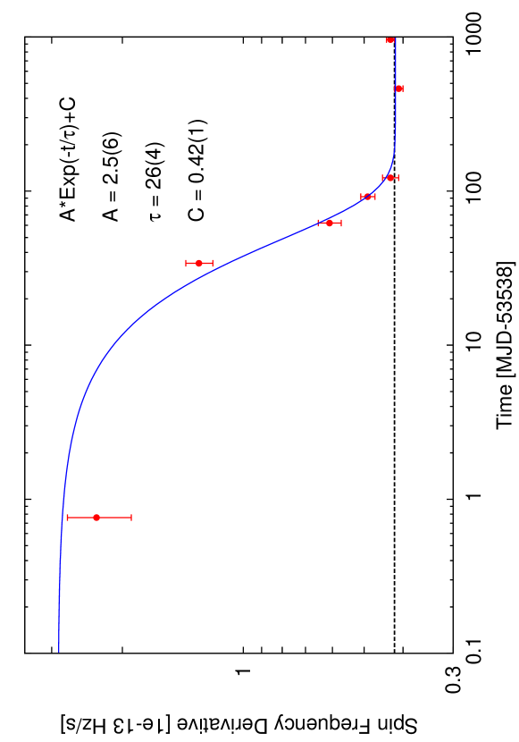
Figure 2.— Evolution of the spin frequency derivative with time. The spin frequency behavior is consistent with an exponential decay with an e-folding time $\tau=26\pm 4$ days and a base level $C=4.2\times 10^{-13}\rm\,Hz\,s^{-1}$.

We find that $\dot{\nu}_{s}$ is clearly changing over time and that it is well described ($\chi^{2}/dof=5.9/4$) by fitting an exponential decay law with a constant level baseline:

$$\dot{\nu}_{s}\left(t\right)=A\,Exp\left(-t/\tau\right)+C$$ (2)

with an e-folding time $\tau=26\pm 4$ days and a constant level $C$ corresponding to a $\dot{\nu}_{s}=4.2\times 10^{-13}\rm\,Hz\,s^{-1}$. The behavior of $\nu_{s}\left(t\right)$ is well described by the integral of the spin frequency derivative:

$$\nu_{s}\left(t\right)=\int\dot{\nu}_{s}\left(t\right)dt=-A\tau Exp\left(-t/\tau\right)+Ct+K$$ (3)

where $K$ is a constant of integration that represents $\nu_{s}$ at the beginning of the outburst. The results for $\dot{\nu}_{s}$ are shown in Figure 2. Given that $\dot{\nu}_{s}$ changes over time we re-fold our data and refit the TOAs considering the different strength of $\dot{\nu}_{s}$ in different intervals but we find no additional pulse episodes.

3.3. Enigmatic Pulse Phase Drift

A very interesting feature is evident in the timing residuals in coincidence with the flare at MJD 53,559. In observation-long pulse profile averages, the pulse phase appears offset by about 0.3 cycles with respect to the phases before the flare (see left panel of Figure 1). After the flare the pulsations disappear for several days and reappear aligned with the phases before the flare. When inspecting 300s to 500s-long pulse profile averages, the pulse phases during the flare show a very fast evolution. The phase starts 0.7 cycles ($250^{\circ}$) offset with respect to the average pulse phase measured in the previous observation (which corresponds to phase 0 in Figure 3) and then drifts back by about 0.5-0.6 cycles ($\sim 180^{\circ}$) towards the phases of the pre-flare observations. In Figure 3 a negative/positive phase residual means that pulsations arrive earlier/later than predicted by the model. An offset of -0.7 cycles is equivalent to an offset of +0.3 cycles, but the interpretation with the negative sign is the correct one because the pulsations show a linear drift with each successive pulsation lagging the previous one. The timescale for the drift is $\approx 3000$ s and pulsations have fractional rms amplitude which remains approximately constant within the statistical errors with a slight excess in the middle of the observation. There, the fractional amplitude reaches 1.6% rms and stays at 1.1% rms in the rest of the observation. The pulsations disappear after this event until MJD 53,573 with 95% c.l. upper limits between 0.35% rms and 1.5% rms. The relatively larger error-bar of the pulse phase obtained by folding the entire data record at the high flux point (as shown in Figure 1) is therefore artificial because the pulse amplitudes are partially smeared out by the fast pulse phase drift.

Figure 3.— Pulse phase drift observed at MJD 53,559. Each data point corresponds to folded lightcurve segments of 300-500 seconds for a total observation time of about 3000 seconds. Negative/positive values correspond to pulsations arriving earlier/later than predicted by the timing model.

4. Discussion

The detection of sporadic pulse episodes in the 2.5 years following the last robust detection at MJD 53,602 strengthens the suggestions of Galloway et al. (2008) that pulsations might be always present in HETE J1900.1–2455. The pulses we detect might represent the “tip of the iceberg” of very weak pulsations that are present at a level of $\lesssim 0.1\%$ rms, since our upper limits reach the most stringent value of about 0.05-0.5% rms. This suggestion is reinforced by our detection of pulses with amplitudes as low as 0.3% rms. Such low values can be reached only because we have an initial timing solution for the orbit and the NS spin which is sufficiently precise to allow a coherent analysis over the entire 7 years of observations. It is not possible, with current instrumentation, to inspect any other non-pulsating LMXB with a comparable X-ray flux and place such extreme upper limits for the pulsed fractions with incoherent timing techniques. Existing upper limits on the pulse fractional amplitudes in non-pulsating LMXBs are usually of the order of 1% rms.

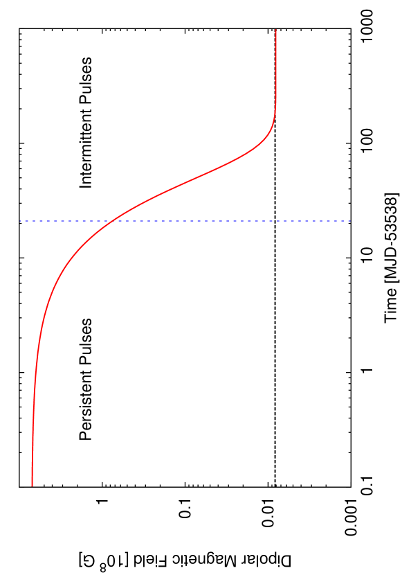
Figure 4.— Evolution of the magnetic field according to Eq.(4) for $\dot{M}_{-10}=10^{-9}\rm\,M_{\odot}\,yr^{-1}$ and an exponentially decaying $\dot{\nu}_{s}$ as shown in Figure 2. The vertical dashed blue line represents the time when pulsations first disappear and corresponds to a field of $7\times 10^{7}$ G.

The baseline available for measuring the spin frequency and the spin-up is $\sim 2.5$ years and this is an unprecedented possibility for AMXPs, since accretion torques have been investigated so far only on relatively short timescales reaching at most $\sim 100$ days (Patruno et al. 2010). The spin up of HETE J1900.1–2455 follows an exponential decay with an e-folding timescale of $26\pm 4$ days and a constant baseline of about $4\times 10^{-13}\rm\,Hz\,s^{-1}$. The spin frequency derivative expected from accretion torques that develop at the disk-magnetosphere boundary of standard thin disks truncated by a constant dipolar magnetic field is:

$$\dot{\nu}_{s}\approx 2.3\times 10^{-14}\xi^{1/2}\dot{M}_{-10}^{6/7}B^{2/7}_{8}M_{1.4}^{-5/21}R_{10}^{6/7}\rm\,Hz\,s^{-1}.$$ (4)

where $\dot{M}_{-10}$ is the mass accretion rate in units of $10^{-10}M_{\odot}/\mbox{yr}$, $B_{8}$ the dipolar magnetic field at the poles in units of $10^{8}$ G, $M_{1.4}$ the mass of the NS in units of $1.4M_{\odot}$, $R_{10}$ its radius in units of $10$ km. The parameter $\xi$ is introduced to account for the uncertainties in the torque at the edge of the accretion disc and is in the range $\xi\approx 0.3-1$ (Psaltis & Chakrabarty 1999).

As noticed by Galloway et al. (2008), the lightcurve of HETE J1900.1–2455 shows an erratic behavior with large variations in X-ray flux on timescales of tens of days. The flux averaged over several tens of days is, however, rather constant (we find variations of at most 20% in X-ray flux between the averages of our seven intervals) and is certainly not exhibiting an exponential drop. Therefore the exponential decay of $\dot{\nu}_{s}$ cannot be related solely with variations in $\dot{M}$ (if we assume that $L_{X}\propto\dot{M}$; see, however,  van der Klis 2001 for a criticism), neither with variations of $M$ and $R$ which stay basically constant throughout the outburst. If the magnetic field is responsible for the variation of $\dot{\nu}_{s}$, then the $B$ field has to decay approximately exponentially with a very short e-folding time of $\sim 10$ days.

Magnetic field burial models predict an exponential decay of the external magnetic field which is screened by freshly accreted plasma (Cumming et al. 2001; Cumming 2008). As matter is accreted to the polar caps it will eventually spread laterally and bury the field underneath. If the new material accumulates on the NS surface on a timescale which is much shorter than the Ohmic diffusion timescale, the magnetic field is (partially) screened. In these models the field suppression operates on timescales that vary significantly and depends on several assumptions. For example, Choudhuri & Konar (2002) have shown that screening timescales of $\sim 1$ yr can be achieved provided that the no magnetic buoyancy is present (see also Payne & Melatos 2004, 2007; Wette et al. 2010). The fact that our fit requires a constant level can also be naturally explained in this scenario by considering that the magnetic field is not efficiently screened once its value is so low that channeled accretion becomes difficult (see Konar & Choudhuri 2004 and compare our Figure 2 with their Figure 10; Zhang & Kojima 2006). Once the outburst is over, the magnetic field can re-emerge on the Ohmic diffusion timescale (Cumming et al. 2001) and return to its initial value of $\sim 10^{8}$ G. For illustrative purposes we plot in Figure 4 the $B$ field at the NS poles of HETE J1900.1–2455 where we use Eq.(4) and assume a constant $\dot{M}_{-10}=10$, $\xi=1$, $M_{1.4}=1$ and $R_{10}=1$. The AMXP has a magnetic field at the beginning of the outburst of $B_{i}\sim 5\times 10^{8}$ G and a final field of $B_{f}\sim 7\times 10^{5}$ G, which is significantly less than the minimum field necessary to truncate the accretion disk (Psaltis & Chakrabarty 1999). This could in principle be related to the extraordinary low rms amplitudes of pulsations in HETE J1900.1–2455.

A similar behavior might not be observed in other persistent AMXPs possibly because of the substantially smaller mass accretion rate which is one to two orders of magnitude lower than in HETE J1900.1–2455. If the timescale for the magnetic screening scales inversely with the mass accretion rate (Konar & Choudhuri 2004) then the magnetic field of persistent AMXPs might require one to several years to substantially decrease. Since the outburst duration of persistent AMXPs is at most 100 days, the screening mechanism cannot reduce the strength of the magnetic field below the level necessary to channel plasma along the field lines.

If magnetic screening is the correct interpretation of our findings, then the anti-correlation between phase and X-ray flux might possibly also be explained with variations of the magnetosphere (and thus on the position of the polar caps) that responds to variations in the amount of accreted material (see also theoretical investigations of this problem in Long et al. 2012; Kajava et al. 2011; Poutanen et al. 2009; Lamb et al. 2009a). However, the anti-correlation does not work on very short timescales of the order of a few hundred seconds. In particular, the sudden $\approx 180^{\circ}$ (0.5 cycles) pulse phase drift observed at MJD 53,559 remains an enigmatic event and it might contain the key to understand why pulsations disappeared for the first time right after this event.

References

- Altamirano et al. (2008) Altamirano, D., Casella, P., Patruno, A., Wijnands, R., & van der Klis, M. 2008, ApJ, 674, L45
- Casella et al. (2008) Casella, P., Altamirano, D., Patruno, A., Wijnands, R., & van der Klis, M. 2008, ApJ, 674, L41
- Choudhuri & Konar (2002) Choudhuri, A. R., & Konar, S. 2002, MNRAS, 332, 933
- Cumming (2008) Cumming, A. 2008, in American Institute of Physics Conference Series, Vol. 1068, American Institute of Physics Conference Series, ed. R. Wijnands, D. Altamirano, P. Soleri, N. Degenaar, N. Rea, P. Casella, A. Patruno, & M. Linares, 152–159
- Cumming et al. (2001) Cumming, A., Zweibel, E., & Bildsten, L. 2001, ApJ
- Dib et al. (2005) Dib, R., Ransom, S. M., Ray, P. S., Kaspi, V. M., & Archibald, A. M. 2005, ApJ, 626, 333
- Edwards et al. (2006) Edwards, R. T., Hobbs, G. B., & Manchester, R. N. 2006, MNRAS, 372, 1549
- Fox (2005) Fox, D. B. 2005, The Astronomer’s Telegram, 526, 1
- Galloway et al. (2008) Galloway, D. K., Morgan, E. H., & Chakrabarty, D. 2008, in American Institute of Physics Conference Series, Vol. 1068, American Institute of Physics Conference Series, ed. R. Wijnands, D. Altamirano, P. Soleri, N. Degenaar, N. Rea, P. Casella, A. Patruno, & M. Linares, 55–62
- Galloway et al. (2007) Galloway, D. K., Morgan, E. H., Krauss, M. I., Kaaret, P., & Chakrabarty, D. 2007, ApJ, 654, L73
- Gavriil et al. (2007) Gavriil, F. P., Strohmayer, T. E., Swank, J. H., & Markwardt, C. B. 2007, ApJ, 669, L29
- Hartman et al. (2008) Hartman, J. M., Patruno, A., Chakrabarty, D., et al. 2008, ApJ, 675, 1468
- Hartman et al. (2009) Hartman, J. M., Patruno, A., Chakrabarty, D., Markwardt, C. B., Morgan, E. H., van der Klis, M., & Wijnands, R. 2009, ArXiv e-prints
- Hobbs et al. (2006) Hobbs, G. B., Edwards, R. T., & Manchester, R. N. 2006, MNRAS, 369, 655
- Kaaret et al. (2006) Kaaret, P., Morgan, E. H., Vanderspek, R., & Tomsick, J. A. 2006, ApJ, 638, 963
- Kajava et al. (2011) Kajava, J. J. E., Ibragimov, A., Annala, M., Patruno, A., & Poutanen, J. 2011, MNRAS, 417, 1454
- Konar & Choudhuri (2004) Konar, S., & Choudhuri, A. R. 2004, MNRAS, 348, 661
- Lamb et al. (2009a) Lamb, F. K., Boutloukos, S., Van Wassenhove, S., Chamberlain, R. T., Lo, K. H., Clare, A., Yu, W., & Miller, M. C. 2009a, ApJ, 706, 417
- Lamb et al. (2009b) Lamb, F. K., Boutloukos, S., Van Wassenhove, S., Chamberlain, R. T., Lo, K. H., & Miller, M. C. 2009b, ApJ, 705, L36
- Long et al. (2012) Long, M., Romanova, M. M., & Lamb, F. K. 2012, New Astronomy, 17, 232
- Özel (2009) Özel, F. 2009, ApJ, 691, 1678
- Papitto et al. (2011) Papitto, A., et al. 2011, A&A, 535, L4
- Patruno (2010a) Patruno, A. 2010a, astro-ph/1007.1108
- Patruno (2010b) —. 2010b, ApJ, 722, 909
- Patruno et al. (2010) Patruno, A., Hartman, J. M., Wijnands, R., Chakrabarty, D., & van der Klis, M. 2010, ApJ, 717, 1253
- Patruno et al. (2009a) Patruno, A., Altamirano, D., Hessels, J. W. T., Casella, P., Wijnands, R., & van der Klis, M. 2009a, ApJ, 690, 1856
- Patruno et al. (2009b) Patruno, A., Wijnands, R., & van der Klis, M. 2009b, ApJ, 698, L60
- Payne & Melatos (2004) Payne, D. J. B., & Melatos, A. 2004, MNRAS, 351, 569
- Payne & Melatos (2007) —. 2007, MNRAS, 376, 609
- Poutanen et al. (2009) Poutanen, J., Ibragimov, A., & Annala, M. 2009, ApJ, 706, L129
- Psaltis & Chakrabarty (1999) Psaltis, D., & Chakrabarty, D. 1999, ApJ, 521, 332
- Romanova et al. (2008) Romanova, M. M., Kulkarni, A. K., & Lovelace, R. V. E. 2008, ApJ, 673, L171
- Titarchuk et al. (2002) Titarchuk, L., Cui, W., & Wood, K. 2002, ApJ
- van der Klis (2001) van der Klis, M. 2001, ApJ, 561, 943
- Vaughan et al. (1994) Vaughan, B. A., et al. 1994, ApJ, 435, 362
- Wette et al. (2010) Wette, K., Vigelius, M., & Melatos, A. 2010, MNRAS, 402, 1099
- Zhang & Kojima (2006) Zhang, C. M., & Kojima, Y. 2006, MNRAS, 366, 137