The Unseen Population of F to K-type Companions to Hot Subdwarf Stars

Abstract

We present a method to select hot subdwarf stars with A to M-type companions using photometric selection criteria. We cover a wide range in wavelength by combining GALEX ultraviolet data, optical photometry from the SDSS and the Carlsberg Meridian telescope, near-infrared data from 2MASS and UKIDSS. We construct two complimentary samples, one by matching GALEX, CMC and 2MASS, as well as a smaller, but deeper, sample using GALEX, SDSS and UKIDSS. In both cases, a large number of composite subdwarf plus main–sequence star candidates were found. We fit their spectral energy distributions with a composite model in order to estimate the subdwarf and companion star effective temperatures along with the distance to each system. The distribution of subdwarf effective temperature was found to primarily lie in the $20,000-30,000$ K regime, but we also find cooler subdwarf candidates, making up $\sim 5-10$ per cent. The most prevalent companion spectral types were seen to be main–sequence stars between F0 and K0, while subdwarfs with M-type companions appear much rarer. This is clear observational confirmation that a very efficient first stable Roche-lobe overflow channel appears to produce a large number of subdwarfs with F to K-type companions. Our samples thus support the importance of binary evolution for subdwarf formation.

1 Introduction

Subluminous blue stars were first discovered by Humason & Zwicky (1947) in a photometric survey of the North Galactic Pole region. Green et al. (1986) found many more hot subdwarfs in the Palomar-Green (PG) survey, to the extent that they were the dominant species among faint ($B\lesssim 16.1$) blue objects. In the PG survey they outnumber white dwarfs (WD) and are prevalent enough to account for the ultraviolet upturn in early-type galaxies (Brown et al., 1997). Hot subdwarf stars are either core helium-burning stars at the end of the horizontal branch or have evolved even beyond that stage (Heber et al., 1984; Heber, 1986). They have a relatively well defined mass around the canonical (theoretical) value of $0.46$ $\mathrm{M}_{\odot}$ (Saffer et al., 1994; Han et al., 2003; Politano et al., 2008) and radii of a few tenths of a solar radius. Their very thin layers of hydrogen ($\mathrm{M}_{\mathrm{env}}<0.01\mbox{$\mathrm{M}_{\odot}$}$) are not able to support shell burning after helium-core exhaustion. Thus instead of following the asymptotic giant branch route, they evolve more or less directly into white dwarfs. Observationally two classes are defined, those with helium-poor spectra (sdBs) and those that are helium-rich (sdOs).

Formation scenarios of subdwarfs invoke either fine-tuned single star evolution or rely on close-binary star interactions. In the late hot-flasher scenario, a low-mass star undergoes the He core-flash at the tip of the red-giant branch. However, if sufficient mass is lost on the red giant branch, the star can experience the He core-flash whilst descending the white dwarf cooling track (Castellani & Castellani, 1993). Such a star would end up close to the He main sequence (MS), at the very hot end of the extreme horizontal branch (D’Cruz et al., 1996). Alternatively, the formation involves one or two phases of common-envelope evolution and/or stable Roche-lobe overflow (RLOF) within a close binary system (Mengel et al., 1976). Binary evolution could even take the route of merging two helium white dwarfs followed by He ignition (Webbink, 1984; Iben, 1990; Saio & Jeffery, 2000). All formation scenarios require substantial mass loss before the start of core He-burning, however the specific physical mechanisms for this are still unclear. A detailed review on this and the field as a whole is given by Heber (2009).

Since the first quantitative estimates of the contribution of different binary channels to the population of subdwarf stars (Tutukov & Yungelson, 1990), it has been shown that a large fraction of subdwarfs do reside in binaries. In the PG sample of subdwarfs, a significant fraction show composite colours or spectra (at least 20 per cent; Ferguson et al. 1984, $\sim 54-66$ per cent; Allard et al. 1994). Radial velocity surveys (e.g. Maxted et al., 2001; Morales-Rueda et al., 2003) confirm the high fraction of binaries with ratios as high as two-thirds. High-resolution optical spectra from the ESO Supernova Ia Progenitor Survey (SPY; Napiwotzki et al., 2001), led to binary star fractions of 30-40 per cent (Napiwotzki et al., 2004; Lisker et al., 2005). Copperwheat et al. (2011) estimate that the binary fraction in the sdB population is somewhat higher at 46 - 56 per cent. This is only a lower limit since the radial velocity variations that Copperwheat et al. (2011) search for would be difficult to detect in long period systems.

Other searches have used near-infrared photometry (e.g. Thejll et al., 1995; Ulla & Thejll, 1998; Williams et al., 2001) or photometric catalogues such as the Two Micron All Sky Survey (2MASS; Skrutskie et al., 2006) to find subdwarfs with companions (e.g. Stark & Wade, 2003; Green et al., 2006; Vennes et al., 2011). Ca II absorption can also be used to infer the presence of a cooler companion star (Jeffery & Pollacco, 1998). The majority of companions found to date have either been M-type stars or white dwarfs (Heber, 2009). However, some F, G and K-type companions to subdwarfs have been seen in studies such as Aznar Cuadrado & Jeffery (2001), Reed & Stiening (2004), Lisker et al. (2005), Wade et al. (2006), Stark & Wade (2006), Wade et al. (2009), Moni Bidin & Piotto (2010) and Geier et al. (MUCHFUSS; 2011b). Depending on the study, and its corresponding selection effects, the companions to subdwarfs have been shown to be mostly main-sequence stars (e.g. Aznar Cuadrado & Jeffery, 2001) and giant or subgiant companions in some cases (e.g. Allard et al. 1994 and BD-$7^{\circ}5977$; Heber et al. 2002).

Many of the previous surveys have been biased by selection effects and inhomogeneous data sets. Han et al. (2003) argued that a large number of sdB stars may be missing from current samples. Early-type main–sequence stars of spectral type A and earlier would outshine a subdwarf at optical wavelengths. F to K-type companions on the other hand, have generally been avoided because the spectral analysis of the composite spectrum becomes difficult. Systems with earlier type companions are actually predicted, in some cases, to be far more common than the M-type companions that have primarily been found so far. In the Han et al. (2003) study, subdwarfs with early type companions are produced in the very efficient first stable RLOF channel and are expected to be in systems with subdwarfs as cool as $15,000$ K. Clausen et al. (2012), however, do not find the same multitude of F-type companions. Identifying this predicted population, and determining their relative contribution to the subdwarf population would offer important constraints on the prior binary evolution that led to their formation. In addition, the distribution of orbital periods and subdwarf temperatures of such a sample will provide direct constraints on key parameters that underpin subdwarf population synthesis models (Clausen et al., 2012).

In this study, we take advantage of recent large-area ultraviolet, optical and infrared photometric surveys to search for new composite systems comprised of subdwarfs plus main–sequence star companions of mid-M-type and earlier. Cuts in colour-colour space are employed to separate these objects from possible contaminants. We also develop a fitting technique to simultaneously determine the subdwarf and companion effective temperatures from the photometric magnitudes. This permits the recovery of composite systems with much earlier type companions than seen in previous studies. Furthermore, we are sensitive to a wide range of separations and binary periods in that we only limit ourselves to spatially unresolved systems. Finally, we discuss the distribution of objects in effective temperature and distance to the system.

2 Synthetic models

To aid our search for subdwarfs with companions, we produced a grid of synthetic sdB and main–sequence star spectra, which allowed us to produce synthetic colours of the composite systems.

The sdB spectra were calculated using the model atmosphere code described by Heber et al. (2000), covering $\mbox{$\mathrm{T}_{\mathrm{eff}}$}=11,000-40,000$ K in steps of $1,000$ K. The corresponding surface gravities were chosen to ensure that our temperature sequence tracks the (extreme) horizontal-branch stars (Dorman et al., 1993). This translates into $\mbox{$\log\,g$}=4.0$ for $\mbox{$\mathrm{T}_{\mathrm{eff}}$}=11,000-13,000$ K objects, $\mbox{$\log\,g$}=4.5$ for $\mbox{$\mathrm{T}_{\mathrm{eff}}$}=14,000-16,000$ K, $\mbox{$\log\,g$}=5.0$ covering $\mbox{$\mathrm{T}_{\mathrm{eff}}$}=17,000-20,000$ K, $\mbox{$\log\,g$}=5.5$ for $\mbox{$\mathrm{T}_{\mathrm{eff}}$}=21,000-28,000$ K and $\mbox{$\log\,g$}=6.0$ for $\mbox{$\mathrm{T}_{\mathrm{eff}}$}=29,000-40,000$ K. Surface gravity does not significantly affect spectral slope, but does affect the width of line profiles, which is a negligible feature when fitting photometry as we do here. It also corresponds to a significant change in the size of the subdwarf and therefore the relative brightness of the subdwarf and the companion.

A range of solar metalicity main–sequence star templates of effective temperatures from $4,250$ K to $25,000$ K in 48 steps were taken from the Castelli & Kurucz (2003) ATLAS9 model atmosphere library. For models below $4,250$ K, Pickles (1998) stellar spectral library models are substituted because of the problems with Castelli & Kurucz (2003) model colours in this region (Bertone et al., 2004). A Pickles (1998) M0V star is used as a proxy for a $4,000$ K model. Similarly, M1V, M2V, M3V and M5V replace $3,750$ K, $3,500$ K, $3,250$ K and $3,000$ K models, respectively. We restrict the models to unevolved main–sequence stars because, as we will see in Section 4.2, sub-giant and giant companions do not contribute significantly to our sample. The impact of this will be further discussed in Sections 7 and 8. Both the sdB and main–sequence star spectra cover the wavelength range $1,150-25,000$ Å. To normalise the Castelli & Kurucz (2003) main–sequence star models to a flux at $10$ pc, we rescale the models to match the luminosities from the (zero age main sequence) isochrones of Girardi et al. (2000).

The two grids of spectra were folded through all relevant filter transmission curves to calculate absolute magnitudes. The two components could therefore be added at a common distance. To separate composite subdwarf plus companion systems from single subdwarfs and single main–sequence stars in colour-colour space, a large wavelength range must be sampled. The combination of a very blue and a red colour allows for a significant contribution from both the subdwarf and companion components to be seen in a colour-colour diagram. We therefore chose to cross-match an ultraviolet survey with a series of optical and near-infrared surveys.

3 Cross-matching

3.1 Sample I: GALEX, CMC and 2MASS

The Carlsberg Meridian Telescope (CMT) has a 2k by 2k CCD camera with a Sloan $r$ filter operating in a drift scan mode. The CMT maps the sky from La Palma (Spain) covering the declination range $-30^{\circ}$ to $+50^{\circ}$ with a magnitude limit of $\mbox{$r_{\mathrm{CMC}}$}=17$. The Carlsberg Meridian Catalogue, Number 14 (Version 1.0: CMC Copenhagen University Obs. et al., 2006) is an astrometric and photometric catalogue of 95.9 million stars covering $9<\mbox{$r_{\mathrm{CMC}}$}<17$. We cross-matched the CMC catalogue with 2MASS using a $2\arcsec$ matching radius. Because the surveys used here avoid the Galactic plane, the contamination from matching to other stars within $2\arcsec$ will be relatively small (Girven et al., 2011). With these combined catalogues, we were able to calculate an $(\mbox{$r_{\mathrm{CMC}}$}-J)$ colour as a diagnostic for spectral type, as well as $(J-K)$, indicative of strong companion star contributions in composite systems (see Figure 1).

Based upon the $(\mbox{$r_{\mathrm{CMC}}$}-J)$ colour of the composite models described in Section 2, the CMC sample was cut to include only stars bluer than a G0V star ($5750$ K on the Castelli & Kurucz 2003 grid), i.e. $(\mbox{$r_{\mathrm{CMC}}$}-J)<0.9$. The cut includes all possible combinations of subdwarf plus companion, but removes a significant fraction of contaminants. This does not limit our selection of subdwarfs with companions as discussed in Section 4. The sample was also limited to $\mbox{$r_{\mathrm{CMC}}$}<16.0$, primarily to match the magnitude limit of 2MASS ($K_{s}\simeq 14.3$). This resulted in $\sim 1.9$ million objects.

All objects within the $(\mbox{$r_{\mathrm{CMC}}$}-J)$ colour cut were cross-matched with the Galaxy Evolution Explorer (GALEX) all-sky ultraviolet survey (Martin et al., 2005) Data Release 6. This provides magnitudes in two bandpasses, $\mathrm{m}_{\mathrm{FUV}}$ and $\mathrm{m}_{\mathrm{NUV}}$, centered around 1500 and 2300Å, respectively. The matching was performed using the predefined cross-matching tables in GALEX CasJobs (Budavári et al., 2009) searching for all sources within $2\arcsec$. The resulting catalogue of neighbours contains approximately $560,000$ matched objects and hereafter will be referred to as the “C2M” sample. The mean of any multiple GALEX observations was taken where available and both bands were corrected for non-linearity according to Morrissey et al. (2007).

Finally, the objects from the match between CMC, 2MASS and GALEX were further cross-matched with the Sloan Digital Sky Survey (SDSS) Data Release 7 (DR7; Abazajian et al., 2009). This sample will hereafter be referred to as the “C2MS” sample which is smaller and photometrically deeper. The SDSS CasJobs predefined cross-matching tables (Li & Thakar, 2008) were utilised. Objects were limited to have good quality photometric magnitudes (see Table 1). This resulted in a sample of $\sim 105,000$ objects for which good SDSS $u$, $g$, $r$, $i$ and $z$ magnitudes were available along with GALEX, CMC and 2MASS photometry. For $\sim 1.5$ per cent of objects within this sample, SDSS optical spectra are available.

Table 1: Colour selection for finding subdwarfs with companions, for both the C2M and C2MS (with or without SDSS magnitudes) and SU samples. Constraints with a “Sample” flag were only applied to that sample, whereas constraints with no flag were applied to both samples. “bad_flags” is defined as saturated or bright or edge or nodeblend and “nChild” is the number of children objects detected by SDSS.

Colour	Constraint		Sample
$r_{\mathrm{CMC}}$	$\leq$	$16.0$	C2M
$(\mbox{$r_{\mathrm{CMC}}$}-J)$	$<$	$0.9$
$r_{\mathrm{CMC}}$ Uncertainty	$\leq$	$0.10$
$\mathrm{E}(\mathrm{B}-\mathrm{V})$	$\leq$	$0.15$
$(\mbox{$\mathrm{m}_{\mathrm{FUV}}$}-\mbox{$r_{\mathrm{CMC}}$})$	$\leq$	$3.8*(\mbox{$r_{\mathrm{CMC}}$}-K_{s})-0.3$
$(\mbox{$\mathrm{m}_{\mathrm{FUV}}$}-\mbox{$r_{\mathrm{CMC}}$})$	$\leq$	$-2.7*(\mbox{$r_{\mathrm{CMC}}$}-K_{s})+4.7$
$(\mbox{$\mathrm{m}_{\mathrm{FUV}}$}-\mbox{$r_{\mathrm{CMC}}$})$	$\geq$	$-3.0$
FUV artifact flag	$\leq$	$1$
$\mathrm{m}_{\mathrm{FUV}}$ Uncertainty	$\leq$	$0.05$	C2M
	$\leq$	$0.10$	SU
	AND
$(\mbox{$\mathrm{m}_{\mathrm{NUV}}$}-\mbox{$r_{\mathrm{CMC}}$})$	$\leq$	$1.3*(\mbox{$r_{\mathrm{CMC}}$}-K_{s})+0.54$
$(\mbox{$\mathrm{m}_{\mathrm{NUV}}$}-\mbox{$r_{\mathrm{CMC}}$})$	$\leq$	$-1.45*(\mbox{$r_{\mathrm{CMC}}$}-K_{s})+3.3$
$(\mbox{$\mathrm{m}_{\mathrm{NUV}}$}-\mbox{$r_{\mathrm{CMC}}$})$	$\leq$	$3.5*(\mbox{$r_{\mathrm{CMC}}$}-K_{s})+0.12$
$(\mbox{$\mathrm{m}_{\mathrm{NUV}}$}-\mbox{$r_{\mathrm{CMC}}$})$	$\geq$	$-2.0$
NUV artifact flag	$\leq$	$1$
$(\mbox{$r_{\mathrm{CMC}}$}-K_{s})$	$\leq$	$1.75$	C2M
$\mathrm{m}_{\mathrm{NUV}}$ Uncertainty	$\leq$	$0.05$	C2M
$(\mbox{$r_{\mathrm{SDSS}}$}-K)$	$\leq$	$1.5$	SU
$\mathrm{m}_{\mathrm{NUV}}$ Uncertainty	$\leq$	$0.10$	SU
SDSS specific:
flags & bad_flags	$=$	$0$
nChild	$=$	$0$

3.2 Sample II: GALEX, SDSS and UKIDSS

The GALEX, CMC and 2MASS cross-matched sample discussed above benefits from covering a large area (limited by the GALEX footprint), but is relatively shallow with a limiting magnitude of $r=16.0$ and $K_{s}=14.3$. This restricts our ability to construct volume-limited samples.

A second, complimentary sample was selected from GALEX, SDSS and UKIDSS. One of the five UKIDSS sub-surveys, the Large Area Survey (LAS), aims to be the infrared counterpart to the SDSS. UKIDSS LAS will eventually provide imaging over $4028\,\deg^{2}$ in four broad band colours, $Y$, $J$, $H$, and $K$, with limiting (Vega) magnitudes of 20.2, 19.6, 18.8 and 18.2, respectively. This adds a significant increase in depth over 2MASS. Here, we made use of UKIDSS Data Release 9 (see Dye et al. 2006), which covers $\sim 60$ per cent of the total, planned, LAS area. SDSS and UKIDSS were cross-matched to find the closest match within $2\arcsec$ using the UKIDSS-SDSS pre-match tables. This sample was then matched to GALEX within $2\arcsec$, using the CasJobs neighbours search, returning approximately $120,000$ objects. Again, multiple GALEX neighbours were combined into a single measurement and fluxes were corrected for non-linearity (Morrissey et al., 2007). This sample will hereafter be referred to as the “SU” sample. It is limited in area by the current size of UKIDSS, but extends several magnitudes deeper than 2MASS in $K$. Because the UKIDSS LAS area is entirely encompassed by the SDSS footprint, we can make use of the higher precision, deeper SDSS photometry, rather than CMC. The number of objects at each stage of the analysis is given in Table 2.

Table 2: Summary of numbers at each stage of the processing. The left hand columns shows which surveys were included at that stage in the processing. The “In cuts” columns are those objects satisfying the criteria from Figure 1 and Table 1 and the “$\Sigma$” column displays the total number of objects in this catagory.

Sample	Surveys				Total	In cuts
Name	Ultraviolet	Optical		Infrared	(approx)	$\Sigma$	SDSS Spectra	SIMBAD
			CMC	2MASS	$1,900,000$	-	-	-
C2M	GALEX		CMC	2MASS	$560,000$	449	-	58
C2MS	GALEX	SDSS	CMC	2MASS	$105,000$	93	25	24
		SDSS		UKIDSS	$220,000$	-	-	-
SU	GALEX	SDSS		UKIDSS	$120,000$	134	72	47

4 Selecting ultraviolet excess objects

4.1 Colour-colour diagrams

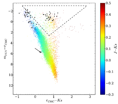
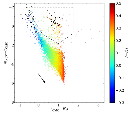
Figure 1: Colour-colour diagrams of $(\mbox{$\mathrm{m}_{\mathrm{FUV}}$}-\mbox{$r_{\mathrm{CMC}}$})$ vs $(\mbox{$r_{\mathrm{CMC}}$}-K_{s})$ (left; $\sim 15,000$ objects) and $(\mbox{$\mathrm{m}_{\mathrm{NUV}}$}-\mbox{$r_{\mathrm{CMC}}$})$ vs $(\mbox{$r_{\mathrm{CMC}}$}-K_{s})$ (right; $\sim 105,000$ objects) for objects with matches in GALEX, CMC and 2MASS catalogues (the C2M sample) and satisfying the magnitude cuts in Table 1. The majority of objects are main–sequence stars and therefore do not have $\mathrm{m}_{\mathrm{FUV}}$ magnitudes. This causes the factor of 10 difference in numbers of objects in the two diagrams. $\mathrm{E}(\mathrm{B}-\mathrm{V})$, taken from the GALEX catalogue Schlegel et al. (1998) map value, is also limited to $<0.15$ and for clarity, $\mbox{$\mathrm{m}_{\mathrm{NUV}}$}\leq 16.5$. The plotted colour for each point corresponds to the $(J-K_{s})$ value, where colours above 0.5 or below -0.3 are shown as 0.5 and -0.3, respectively. For single stars, this range corresponds to spectral types O5 to K0. The sdB/sdO star candidates from Kilkenny et al. (1988) with matches in the C2M catalogue are shown as black circles (totalling 84 objects). A reddening vector corresponding to $\mbox{$\mathrm{E}(\mathrm{B}-\mathrm{V})$}=0.15$ is shown as a black arrow centered on $(0,5)$ in both diagrams. The dashed black lines show the colour-colour selections as discussed in Section 4.2 and Table 1.

Figure 1 shows colour-colour diagrams for the objects with detections in GALEX, CMC and 2MASS. We compare $(\mbox{$\mathrm{m}_{\mathrm{FUV}}$}-\mbox{$r_{\mathrm{CMC}}$})$ vs $(\mbox{$r_{\mathrm{CMC}}$}-K_{s})$ and $(\mbox{$\mathrm{m}_{\mathrm{NUV}}$}-\mbox{$r_{\mathrm{CMC}}$})$ vs $(\mbox{$r_{\mathrm{CMC}}$}-K_{s})$, where the $(J-K_{s})$ colour of each object is colour-encoded in the plot. For single stars, the $(J-K_{s})$ range corresponds to spectral types O5 to K0. The colour indices are tailored to highlight in colour-colour space the position of composite blue plus red objects. The $(\mbox{$r_{\mathrm{CMC}}$}-K_{s})$ colour of an object is a relatively good indication of stellar spectral type and $(\mbox{$\mathrm{m}_{\mathrm{FUV}}$}-\mbox{$r_{\mathrm{CMC}}$})$ will indicate objects with an excess in the ultraviolet in contrast to single main–sequence stars. The truncation at $(\mbox{$r_{\mathrm{CMC}}$}-K_{s})\sim 1.5$ is caused by our imposed cut of $(\mbox{$r_{\mathrm{CMC}}$}-J)<0.9$.

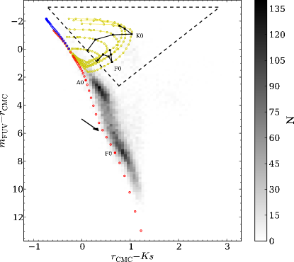
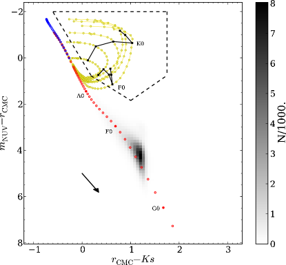
Figure 2: 2D density plots of the $(\mbox{$\mathrm{m}_{\mathrm{FUV}}$}-\mbox{$r_{\mathrm{CMC}}$})$ vs $(\mbox{$r_{\mathrm{CMC}}$}-K_{s})$ and $(\mbox{$\mathrm{m}_{\mathrm{NUV}}$}-\mbox{$r_{\mathrm{CMC}}$})$ vs $(\mbox{$r_{\mathrm{CMC}}$}-K_{s})$ colour-colour diagrams in Figure 1, however, $\mathrm{m}_{\mathrm{NUV}}$ is no longer limited to $16.5$. The grey scale is shown on the respective colour bars, labelled by the number of objects (N) on the left and N/1000 on the right. The reddening vector again corresponds to $\mbox{$\mathrm{E}(\mathrm{B}-\mathrm{V})$}=0.15$ and is shown as a black arrow centered on $(0,5)$. The dashed black lines show the colour-colour selections as discussed in Table 1. Additionally, subdwarf ($15,000\leq\mbox{$\mathrm{T}_{\mathrm{eff}}$}\leq 40,000$ K) and main–sequence star model colours (Section 2) are plotted as blue and red open circles, respectively. The yellow lines show a single subdwarf ($15,000\leq\mbox{$\mathrm{T}_{\mathrm{eff}}$}\leq 40,000$ K in steps of $5,000$ K) paired with the sequence of main–sequence stars described in Section 2. As a reference, subdwarfs (of the above temperatures) with approximately a K0 or F0-type companion are joined with a black line.

In Figure 2, the same sources are plotted but now encoding the density of sources on a grey scale to better represent relative numbers. The main sequence is found along the bottom edge of the main group of objects in the $(\mbox{$\mathrm{m}_{\mathrm{FUV}}$}-\mbox{$r_{\mathrm{CMC}}$})$ vs $(\mbox{$r_{\mathrm{CMC}}$}-K_{s})$ plane, and more centrally through the main group in the $(\mbox{$\mathrm{m}_{\mathrm{NUV}}$}-\mbox{$r_{\mathrm{CMC}}$})$ vs $(\mbox{$r_{\mathrm{CMC}}$}-K_{s})$ plane (Figure 1). Simulated colours derived from our main–sequence star model (Section 2) confirm that this is the expected position of the main sequence in our chosen colours. Similarly, composite sdB plus companion star models are also shown in Figure 2, highlighting the region of colour-colour space where we expect to find such systems.

The large scatter in $(\mbox{$\mathrm{m}_{\mathrm{FUV}}$}-\mbox{$r_{\mathrm{CMC}}$})$ or $(\mbox{$\mathrm{m}_{\mathrm{NUV}}$}-\mbox{$r_{\mathrm{CMC}}$})$ for a given $(\mbox{$r_{\mathrm{CMC}}$}-K_{s})$, especially at the red end, can be explained due to a few factors. First of all, even though we formally require the $r_{\mathrm{CMC}}$ uncertainty to be less than $0.1$, there appears to be additional systematic scatter in the $r_{\mathrm{CMC}}$ magnitudes. Investigating the vertically extended regions in our colour-colour diagrams (Figure 1) when using the much more reliable $r_{\mathrm{SDSS}}$ instead of $r_{\mathrm{CMC}}$, we find that the spread is significantly reduced. However, the larger sky coverage of the CMC is far more important for our study especially as the subdwarf plus companion systems fall in a relatively clean part of the diagram. Another reason for the observed spread is the fact that the GALEX magnitudes have been shown to suffer from non-linearities for bright stars, amongst other problems (e.g. Morrissey et al., 2007; Wade et al., 2009). Although we corrected for non-linearity using the method described in Morrissey et al. (2007), the equations are empirical and there may be a significant scatter in individual measurements.

In addition, despite limiting $\mbox{$\mathrm{E}(\mathrm{B}-\mathrm{V})$}\leq 0.15$, much of the spread around the main sequence can be accounted for by considering the effects of interstellar reddening. The $\mathrm{E}(\mathrm{B}-\mathrm{V})$ magnitude for each object is taken from the GALEX catalogue, which is itself calculated from the Galactic reddening maps of Schlegel et al. (1998). The interstellar reddening is illustrated by the reddening vectors in Figure 1. These are calculated by folding the mean extinction curve of Fitzpatrick & Massa (2007) through the relevant filter transmission curves. In the $(\mbox{$\mathrm{m}_{\mathrm{FUV}}$}-\mbox{$r_{\mathrm{CMC}}$})$ vs $(\mbox{$r_{\mathrm{CMC}}$}-K_{s})$ plane, reddening of blue objects moves them above the main sequence in $(\mbox{$\mathrm{m}_{\mathrm{FUV}}$}-\mbox{$r_{\mathrm{CMC}}$})$, a region populated by a number of objects. However, reddening in the $(\mbox{$\mathrm{m}_{\mathrm{NUV}}$}-\mbox{$r_{\mathrm{CMC}}$})$ vs $(\mbox{$r_{\mathrm{CMC}}$}-K_{s})$ plane approximately moves objects along the main sequence. The components of the reddening vectors are approximately the same in both $(\mbox{$\mathrm{m}_{\mathrm{FUV}}$}-\mbox{$r_{\mathrm{CMC}}$})$ and $(\mbox{$\mathrm{m}_{\mathrm{NUV}}$}-\mbox{$r_{\mathrm{CMC}}$})$ because of the $2200$Å bump in the reddening function (Papoular & Papoular, 2009) coincides with the central wavelength of $\mathrm{m}_{\mathrm{NUV}}$. However, the intrinsic and significant variations in the reddening law along different lines of sight affect the ultraviolet magnitudes more so than the optical values. Fitzpatrick & Massa (2007) show that even when considering the standard stars that are used to calculate the adopted reddening function, a significant spread around the mean extinction curve is observed. This leads to large departures from the mean law, affecting the ultraviolet region in particular. These variations in the extinction curve, along with the variation of the true reddening to the subdwarf compared with that calculated in the Schlegel et al. (1998) maps, are thus likely responsible for the stellar sources populating a vertically extended region in the $(\mbox{$\mathrm{m}_{\mathrm{NUV}}$}-\mbox{$r_{\mathrm{CMC}}$})$ vs $(\mbox{$r_{\mathrm{CMC}}$}-K_{s})$ plane. In any case, the outliers form only a small fraction of the total source population and the reddening vector does not move main–sequence stars into the colour selections we discuss below.

4.2 Isolating subdwarfs in binaries

In order to classify our sources and check for known objects within our sample, we resolved all positions using SIMBAD, and also consulted any available SDSS optical spectra. In the upper-left corner of the $(\mbox{$\mathrm{m}_{\mathrm{FUV}}$}-\mbox{$r_{\mathrm{CMC}}$})$ vs $(\mbox{$r_{\mathrm{CMC}}$}-K_{s})$ colour-colour diagram, one would expect to find white dwarfs and single-star subdwarfs, which is corroborated by classifications in the SIMBAD database. Unfortunately, none of our sources with colours consistent with single subdwarfs have SDSS spectra that could conclusively confirm their classification (due to them saturating in SDSS). The objects towards the right of the diagram, with $(\mbox{$r_{\mathrm{CMC}}$}-K)\sim 2.0$, prove to be galaxies. These are removed by use of the point source flag in SDSS.

Kilkenny et al. (1988) created a catalogue of subdwarf stars and candidates from previous studies, including work on the PG survey. This includes subdwarfs both with and without companions. We matched this catalogue to the C2M catalogue, resulting in 1704 objects. The subset for which appropriate quality limits are satisfied are plotted in Figure 1 (84 sources). We see that this sample splits into two distinct groups. A significant fraction falls in the region where single subdwarfs and white dwarfs are expected to lie. However, a good number of these ($\sim 35$ per cent) lie at a much redder $(\mbox{$r_{\mathrm{CMC}}$}-K_{s})$ colour, where, from the synthetic magnitudes calculated in Section 2, we expect subdwarfs with main–sequence star companions. The objects in this redder region (inside the black dashed lines in Figures 1 and 2), would appear to be main–sequence F or G-type stars from their $(\mbox{$r_{\mathrm{CMC}}$}-K_{s})$ colour, but have an ultraviolet excess in $(\mbox{$\mathrm{m}_{\mathrm{FUV}}$}-\mbox{$r_{\mathrm{CMC}}$})$ and/or $(\mbox{$\mathrm{m}_{\mathrm{NUV}}$}-\mbox{$r_{\mathrm{CMC}}$})$ colour. This confirms that a significant fraction of the Kilkenny et al. (1988) sample show photometric evidence for being composite, but also that we have detected a large number of new sources within that same region of colour space.

For the new C2M objects in this region, where SDSS spectra are available, they can be seen to be mostly subdwarfs along with one white dwarf and two cataclysmic variable stars (CV: see Table 3). SIMBAD, however, only returns four known subdwarfs in this region of colour-colour space. This may be expected as previous work has intentionally focused on single-lined sdB systems that are therefore dominated by the subdwarf. The number of objects grouped under a few broad classifications are summarised in Table 3. Note that close to $90$ per cent of the C2M sources (without SDSS) within this region are unknown.

In order to isolate composite subdwarfs while avoiding obvious contaminants, we devised cuts in colour-colour space (Table 1) guided by our simulated composite subdwarf colours and the SIMBAD and SDSS spectroscopic classifications discussed above. The right hand side of the cuts was chosen to avoid contamination from galaxies and quasars, and similarly on the lower side the main sequence was avoided. At the left hand edge, the cuts were chosen to avoid early-type stars and single subdwarfs. We require objects to be in both the $(\mbox{$\mathrm{m}_{\mathrm{FUV}}$}-\mbox{$r_{\mathrm{CMC}}$})$ vs $(\mbox{$r_{\mathrm{CMC}}$}-K_{s})$ and $(\mbox{$\mathrm{m}_{\mathrm{NUV}}$}-\mbox{$r_{\mathrm{CMC}}$})$ vs $(\mbox{$r_{\mathrm{CMC}}$}-K_{s})$ cuts because objects residing in just an individual box are likely to arise from spurious GALEX fluxes. Contamination of this region due to interstellar reddening is small because very few objects will be moved from the main sequence, along the reddening vector, into the box, as shown in Figure 1. Similarly, the scatter from a poor $r_{\mathrm{CMC}}$ magnitude does not lead to a large contamination, because the subdwarfs with companions region is sufficiently far from the main sequence.

Table 3: Table of classifications for the 449, 93 and 134 objects in the C2MS, C2MS and SU samples, respectively, and inside the colour-colour selection boxes from Figure 1 and Table 1. The SDSS spectra column is from visual inspection of the optical spectra. The number of galaxies seen in the SDSS spectra is virtually zero because the flags used to select the SDSS objects remove any extended objects.

	C2M	C2MS		SU
Classification	SIMBAD	SIMBAD	SDSS spectra	SIMBAD	SDSS spectra
SD	7	4	22	7	62
Composite	9	1	0	4	0
CV/Nova	21	8	2	10	4
Galaxy	2	0	0	0	2
Quasar	0	0	0	0	0
WD	19	11	1	26	4
Total with classification	58	24	25	47	72
Total without classification	391	69	68	87	62

We repeated a similar selection using the SU sample, again using $(\mbox{$\mathrm{m}_{\mathrm{FUV}}$}-\mbox{$r_{\mathrm{SDSS}}$})$ vs $(\mbox{$r_{\mathrm{SDSS}}$}-K)$ and $(\mbox{$\mathrm{m}_{\mathrm{NUV}}$}-\mbox{$r_{\mathrm{SDSS}}$})$ vs $(\mbox{$r_{\mathrm{SDSS}}$}-K)$ colour-colour diagrams (not shown). All magnitudes were limited to have uncertainties less than 0.1 mag and $\mbox{$\mathrm{E}(\mathrm{B}-\mathrm{V})$}\leq 0.15$. An increase in the number of quasars was seen, which encroached on the cuts used for $(\mbox{$\mathrm{m}_{\mathrm{NUV}}$}-\mbox{$r_{\mathrm{CMC}}$})$ vs $(\mbox{$r_{\mathrm{CMC}}$}-K_{s})$. The upper limit on $(\mbox{$r_{\mathrm{SDSS}}$}-K)$ was therefore reduced, as shown in Table 1, however the contamination was not completely removed. The cuts on $(\mbox{$\mathrm{m}_{\mathrm{FUV}}$}-\mbox{$r_{\mathrm{SDSS}}$})$ vs $(\mbox{$r_{\mathrm{SDSS}}$}-K)$ remained unchanged, where we ignore the small differences between UKIDSS $K$ magnitude versus 2MASS $K_{s}$ magnitudes. After these adjustments, 134 objects reside within the cuts, 72 of which have SDSS spectra. This is significantly more than the C2MS sample because many of the C2MS objects are saturated in SDSS. As for the 2MASS sample, we provide broad classifications for the SU sample in Table 3.

With our selection cuts in place, we can use the tracks of our synthetic subdwarf-companion pairs to consider the completeness of our composite subdwarf sample. We find that our region covers only a limited range in companion type for a given subdwarf temperature, as systems that are either dominated by the companion or the subdwarf fall outside our region. This choice is required to reduce contamination from single stars. Based on our simulated colours, we find that subdwarfs with temperatures up to $30,000$ K would fall in the $(\mbox{$\mathrm{m}_{\mathrm{FUV}}$}-\mbox{$r_{\mathrm{CMC}}$})$ vs $(\mbox{$r_{\mathrm{CMC}}$}-K_{s})$ colour cut for even the coolest main–sequence companion in our grid ($3,000$ K: $\sim$M5). $35,000$ K and $40,000$ K subdwarfs, however, would require $\gtrsim 3,750$ K ($\lesssim$M0) and $\gtrsim 5,000$ K ($\lesssim$ K0) companions, respectively, to make them stand out from the main sequence populations. In the case of early-type companions, subdwarfs plus O-type and B-type stars are also lost as they merge back into the blue end of the main sequence. A $15,000$ K, $20,000$ K, $30,000$ K and $40,000$ K subdwarf would be identified if it had an $\lesssim 7,500$ K ($\gtrsim$F0), $\lesssim 8,250$ K ($\gtrsim$A5), $\lesssim 8,000$ K ($\gtrsim$A5) or $\lesssim 8,500$ K ($\gtrsim$A5) companion, respectively.

For the colour-colour tracks, the companions are restricted to be main–sequence stars. However, we may also expect to find a population of subdwarfs with sub-giant or giant companions similar to HD 185510 (Fekel & Simon, 1985), HD 128220 (Howarth & Heber, 1990) and BD-$7^{\circ}5977$ (Viton et al., 1991; Heber et al., 2002). In fact, the binary population synthesis of Han et al. (2003) predicted that the majority of K-type companions to subdwarfs should be evolved companions. We calculated the $(\mbox{$\mathrm{m}_{\mathrm{FUV}}$}-\mbox{$r_{\mathrm{CMC}}$})$ vs $(\mbox{$r_{\mathrm{CMC}}$}-K_{s})$ location of G7 to K3-type giant stars (Figure 3: upper-right panel) by taking the solar metalicity, zero age horizontal branch stars from the Castelli & Kurucz (2003) model atmosphere library and again rescaling the fluxes to a corresponding zero age horizontal branch luminosity from the isochrones of Girardi et al. (2000). All combinations of subdwarf plus giant star systems fall outside of the colour cuts described in Table 3. Systems with either overluminous subdwarfs, or companions in an intermediate state between the main-sequence and the horizontal branch may, however, fall within the colour cuts. We do not expect these to be a significant population in our sample. Since we do not expect specific formation mechanisms to become more or less prevalent as a function of distance, we can still use our sample to study the spatial distribution of subdwarfs even if the sub-sample of subdwarfs with evolved companions is selected against.

We may also expect that some detached white dwarf plus main–sequence type companion systems are found to be contaminants of the sample, since these are composite systems with a hot component and a cooler companion. However, we simulated the colours of such systems and, with the exception of very low gravity white dwarfs, they do not fall in the colour-colour region selected in Table 3 (see Figure 3: lower two panels). In this colour space, the small radius of the white dwarf means that the flux is dominated by all but the latest of main sequence companions and so they lie closer to the main sequence in both diagrams. They are thus unlikely to constitute a significant contaminant.

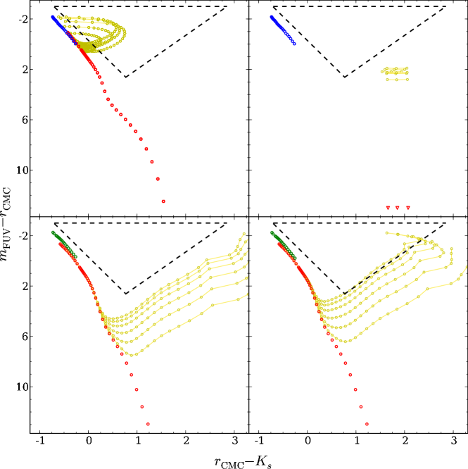
Figure 3: Potential contaminants of the subdwarf plus main–sequence star sample, following the same format as Figure 2. See Section 4.2 for a discussion. Top-left: Subdwarfs (blue open circles: described in Section 2) with metal-poor ($\log([\mathrm{M/H}]/[\mathrm{M/H}]_{\mathrm{solar}})=1.5$: red open circles) main–sequence star companions. Composite objects are shown in yellow. Top-right: Subdwarfs with giant star companions (ranging in spectral type from approximately G7 to K3). Single G and K-type stars do not fall in the range of the Figure, and therefore we mark their $(\mbox{$r_{\mathrm{CMC}}$}-K_{s})$ position by downward pointing red triangles. Bottom-left: $\log(g)=8$ DA white dwarfs (green open circles) with main–sequence companion stars (described in Section 2). Bottom-right: $\log(g)=7$, and therefore larger radii, DA white dwarfs with main–sequence companion stars. The DA white dwarf model grid was kindly provided by D. Koester (for a description, see Koester, 2010), and ranges from $15,000\leq\mbox{$\mathrm{T}_{\mathrm{eff}}$}\leq 40,000$ K in steps of $5,000$ K.

Looking out of the Galactic plane to distances of over $1$ kpc, we may expect to see a sizeable fraction of thick disk and halo stars. Therefore, the companions to the subdwarfs in our samples may be metal-poor. In Figure 3 (upper-left panel), we show that subdwarfs with metal-poor ($\log([\mathrm{M/H}]/[\mathrm{M/H}]_{\mathrm{solar}})=1.5$: ATLAS9: Castelli & Kurucz 2003) companions indeed still fall in our colour selection. We discuss the associated possible biases on our fitting technique in Section 6.

A summary of our sample sizes at various stages of the analysis can be found in Table 2. The full list of 449 objects inside our C2M sample can be found in Table Acknowledgements.

5 Spectroscopic Observations

We discuss here some spectroscopic follow-up obtained to verify that the C2M sample objects likely contain a subdwarf component before turning to the modelling of their spectral energy distributions (SED) in Section 6.

5.1 WHT

Nine objects falling within the colour-colour cuts described in Table 1 were observed in July and December 2010, using the 4.2m William Herschel Telescope (WHT) at the Roque de los Muchachos Observatory, La Palma, Spain. We used the ISIS dual-beam spectrograph mounted at the Cassegrain focus of the telescope, with a R600 grating on both the blue and the red arms, and a 1″  slit. The blue arm of the spectrograph is equipped with a $2048\times 4096$ pixel EEV12 CCD, which we binned by factors of 3 (spatial direction) and 2 (spectral direction). The $2048\times 4096$ pixel REDPLUS CCD on the red arm was binned similarly. This setup delivers a wavelength coverage of $3772-5136$Å  on the blue arm, with an average dispersion of 0.88Å  per binned pixel, and $5983-7417$Å  on the red arm, with an average dispersion of 0.98Å  per binned pixel. We determined the resolution to be 1.2Å, from measurements of the full width at half maximum of night-sky lines. The setup during the December observations was identical, except that the CCDs were binned $2\times 2$.

The spectra were debiased and flatfielded using the starlink packages kappa and figaro and then optimally extracted using the pamela code (Marsh, 1989). We derive the wavelength calibration from Copper-Neon and Copper-Argon arc lamp exposures taken during the night, selecting the arc lamp exposure nearest in time to each science spectrum.

Finally, the raw spectra were converted to flux units and the telluric absorption lines removed. For the July run, the flux calibration was done using a model spectrum of a “flux standard” DA white dwarf, observed on the same night. The December run suffered from poor weather and no flux standard was observed. We calibrated these two spectra using an earlier observation of SP1446+259, taken with the same instrumental setup. The shape of the spectrum is therefore reliable, but the absolute flux level is not. Our analysis does not depend on the absolute flux of the targets, so our conclusions are unaffected.

We plot the resultant spectra in Figure 4 and find that all but one of the nine objects chosen from the colour-colour selection are sdB stars with companions (Table 4).

Table 4: Follow-up spectroscopic observations and classifications.

Name	R.A.	Dec	$r_{\mathrm{CMC}}$	Classification	Telescope
			[mag]
0018$+$0101	$00^{\rm h}18^{\rm m}43.51^{\rm s}$	$+01^{\circ}01^{\prime}23\aas@@fstack{\prime\prime}6$	15.1	sdB	WHT
0051$-$0955	$00^{\rm h}51^{\rm m}20.33^{\rm s}$	$-09^{\circ}55^{\prime}23\aas@@fstack{\prime\prime}2$	14.4	A-type star	WHT
1602$+$0725	$16^{\rm h}02^{\rm m}09.07^{\rm s}$	$+07^{\circ}25^{\prime}10\aas@@fstack{\prime\prime}9$	14.7	sdB	WHT
1618$+$2141	$16^{\rm h}18^{\rm m}06.46^{\rm s}$	$+21^{\circ}41^{\prime}25\aas@@fstack{\prime\prime}4$	14.9	sdB	WHT
1619$+$1453	$16^{\rm h}19^{\rm m}49.30^{\rm s}$	$+14^{\circ}53^{\prime}09\aas@@fstack{\prime\prime}9$	14.7	sdB	WHT
2020$+$0704	$20^{\rm h}20^{\rm m}27.21^{\rm s}$	$+07^{\circ}04^{\prime}13\aas@@fstack{\prime\prime}5$	14.3	sdB	WHT
2047$-$0542	$20^{\rm h}47^{\rm m}42.37^{\rm s}$	$-05^{\circ}42^{\prime}31\aas@@fstack{\prime\prime}0$	14.9	sdB	WHT
2052$-$0457	$20^{\rm h}52^{\rm m}26.23^{\rm s}$	$-04^{\circ}57^{\prime}45\aas@@fstack{\prime\prime}3$	14.5	sdB	WHT
2138$+$0442	$21^{\rm h}38^{\rm m}00.82^{\rm s}$	$+04^{\circ}42^{\prime}11\aas@@fstack{\prime\prime}6$	14.8	sdB	WHT
2331$-$2515	$23^{\rm h}31^{\rm m}03.65^{\rm s}$	$-25^{\circ}15^{\prime}47\aas@@fstack{\prime\prime}9$	14.5	sdB	MagE
2342$-$2750	$23^{\rm h}42^{\rm m}41.41^{\rm s}$	$-27^{\circ}50^{\prime}01\aas@@fstack{\prime\prime}7$	15.1	sdB	MagE

Figure 4: WHT optical spectra of nine candidate subdwarf plus companion stars chosen from the colour-colour selection seen in Figure 1. Eight of the nine targets are subdwarfs with hints of absorption lines from the companion star (see also Section 4). Spectra are ordered approximately by effective temperature of the subdwarf, and shifted in flux by appropriate amounts. 0051$-$0955 is probably an A-type star rather than a subdwarf.

5.2 MagE

In addition to the WHT spectra, two candidates were observed on 7-8 June 2010, using the MagE (Magellan Echellette) spectrograph mounted on the Magellan-Clay telescope at Las Campanas Observatory, Chile. We used the $1\arcsec$ slit with the 175 lines/mm grating to cover $\sim 3100-11200$ Å at a resolution of $R=4100$. The data were unbinned and we used the slow readout mode.

The spectra were reduced with the Carnegie pipeline written by D. Kelson. This Python-driven pipeline performs typical calibrations: flat-fielding, sky background subtraction followed by optimal extraction and wavelength calibration. The wavelength calibrations were derived from Thorium-Argon lamp exposures taken during the night, which provided ample suitable lines over the entire wavelength range. The pipeline selects the closest lamp exposures in time to each science spectrum. Raw spectra were then flux calibrated using a spectrum of the flux standard Feige 110, observed at the end of each night. We find that both objects observed have spectra consistent with being sdB stars with some evidence for a companion.

This initial exploration of eleven of our candidates thus offers strong evidence that we are primarily selecting composite subdwarf systems with our colour cuts, with a low contamination rate. We discuss contamination of our samples further in Sections 7.8 and 7.9.

6 Fitting composite systems

To quantify the likely composition of our subdwarf candidates, we pursued SED fitting exploiting the broad wavelength range of the photometric data that is available. The subdwarf star dominates the ultraviolet flux while the main–sequence companion clearly dominates in the infrared. This permits the decomposition of the SED into two components at a common distance. In this section we demonstrate that good constraints on both the subdwarf and companion star effective temperature can be derived from such fits. The observed magnitudes were fitted with the grid of subdwarf plus main–sequence star magnitudes discussed in Section 2, with the additional option of having a subdwarf with no companion (shown as MS $\mbox{$\mathrm{T}_{\mathrm{eff}}$}=0$ K in Table 5 onwards). This was performed by minimising a weighted $\chi^{2}$ whilst varying the distance, subdwarf and companion effective temperatures. Uncertainties were taken from the one sigma contours in the $\chi^{2}$ surface. This fitting was restricted to the sub-samples where SDSS photometry is available, since we require multi-band optical photometry in order to decompose the SED.

Reddening from interstellar dust can potentially have a significant effect on the shape of the subdwarf SED, especially at short wavelengths. It would therefore primarily affect the inferred subdwarf effective temperature. The slope will be flattened and thus a systematically lower effective temperature would be found. Without prior knowledge of the reddening to the system, this is not easily corrected for. To estimate an upper limit for this effect, we calculate the reddening at the position of the subdwarfs from the Schlegel et al. (1998) maps and use these values to first deredden the magnitudes. Refitting these values gives a second set of system parameters that will, in general, be overcorrected for reddening in comparison to the fits without any reddening. The true parameters will lie somewhere in between these two limits.

As shown in Figure 3, subdwarfs with metal-poor companions fall in the colour cuts defined in Table 3. They are not a contaminant, but fitting the metal-poor systems with solar metalicity models will lead to biased system parameters. Less absorption in the ultraviolet from metal lines means the companions will contribute a fairly significant amount of flux at short wavelengths. To test the effect of this, we fitted the C2MS and SU samples with a grid of subdwarfs plus metal-poor ($\log([\mathrm{M/H}]/[\mathrm{M/H}]_{\mathrm{solar}})=1.5$) companions from the Castelli & Kurucz (2003) ATLAS9 model atmosphere library. This has the effect of reducing all subdwarf effective temperatures by a few thousand Kelvin and shifting the distribution of companion types later by a few hundred Kelvin. If anything, this accentuates the conclusions we draw in Section 8.

A final potential bias to our fitting method is that approximately $10$ per cent of subdwarfs are evolved and therefore will have lower surface gravities and bloated radii compared with their unevolved equivalent (Heber, 2009). Fitting a system with an evolved subdwarf using our subdwarf plus main–sequence star model grid (described in Section 2), we would find that the companion star is cooler and the subdwarf is hotter than the true temperature. However, this situation will most likely result in a high minimum $\chi^{2}$ and therefore be flagged as a bad fit.

7 Fit Results and Individual Objects

All the fit parameters for the 93 objects from the C2MS sample (Table 2) are given in Table 10. Similarly, the 134 SU objects are shown in Table 13. We adopt a somewhat unusual notation for the upper and lower uncertainties, denoted by the “{” symbol, because the subdwarf and companion effective temperature uncertainties are strongly correlated. “{” indicates the upper and lower $1\sigma$ uncertainties added to the best fit value. The upper values all correspond to the same fit solution and similarly for the lower values. As an example, consider a hypothetical system where SD $\mbox{$\mathrm{T}_{\mathrm{eff}}$}=15,000\{^{25,000}_{10,000}$ K, and MS $\mbox{$\mathrm{T}_{\mathrm{eff}}$}=2,000\{^{1,000}_{3,000}$ K. This corresponds to three solutions: the best fit (a $15,000$ K subdwarf with a $2,000$ K companion), a $1\sigma$ uncertainty in the direction of increased subdwarf temperature (a $25,000$ K subdwarf with a $1,000$ K companion), and a $1\sigma$ uncertainty in the direction of decreased subdwarf temperature (a $10,000$ K subdwarf with a $3,000$ K companion). One cannot mix and match these combinations. For example, a $10,000$ K subdwarf with a $1,000$ K companion, or a $25,000$ K subdwarf with a $3,000$ K companion, are not valid solutions. A minimum uncertainty is set at one grid point and therefore is also limited by the extent of the grid: a minimum and maximum subdwarf temperature of $11,000$ and $40,000$ K, respectively. We examine systematic uncertainties in Section 7.8, leading to estimates of a few thousand Kelvin for a more realistic error. We show example SEDs and fits to a few objects in Figures 5 and 6. Objects in Figures 5 and 6 are found to have approximately G0 and A7-type companions, respectively.

We compared our results to published effective temperatures and/or known companions for the C2MS and SU samples, shown in Table 5 and 6, respectively. The best fit is not always satisfactory, indicated by a high $\chi^{2}$. We include the “Q” (Quality) column to show where this is the case. “Q” values correspond to; 1:Good fit, 2:Average fit, 3:Poor fit, 4:WD/WD+MS/CV and 5:Quasar/Galaxy. Values of three and above are excluded from the histograms shown in Figure 8, 9 and 10. The classifications in this catagory between values of 1, 2 and 3 are purely qualitative. SIMBAD has an entry for many more objects, but without any specific details. All objects which were previously known (in one or more of: Ferguson et al. 1984, Kilkenny et al. 1988, Allard et al. 1994, Saffer et al. 1994, Thejll et al. 1995, Ulla & Thejll 1998, Jeffery & Pollacco 1998, Aznar Cuadrado & Jeffery 2001, Maxted et al. 2001, Williams et al. 2001, Aznar Cuadrado & Jeffery 2002, Maxted et al. 2002, Edelmann et al. 2003, Morales-Rueda et al. 2003, Stark & Wade 2003, Napiwotzki et al. 2004, Reed & Stiening 2004, Lisker et al. 2005, Østensen 2006, Wade et al. 2006, Stark & Wade 2006, Stroeer et al. 2007, Wade et al. 2009, Geier et al. 2011a and Vennes et al. 2011 ) to be composite subdwarf plus companion systems are highlighted in Tables 10 and 13.

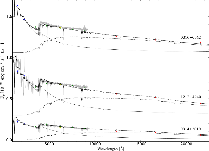
Figure 5: The SEDs of, and fits to, 0316$+$0042 (PG 0313$+$005), 0814$+$2019 and 1212$+$4240 (PG 1210$+$429). The optical SDSS spectra are shown in grey. The GALEX, SDSS, CMC and 2MASS magnitudes are plotted in blue, green, yellow and red, respectively with corresponding errorbars. The fit to 0316$+$0042 comprises a $\mbox{$\mathrm{T}_{\mathrm{eff}}$}=28,000$ K sdB model and a $6,250$ K star (black dashed lines). Similarly, a $\mbox{$\mathrm{T}_{\mathrm{eff}}$}=21,000$ K sdB model and a $5,500$ K star is used for 0814$+$2019 and a $\mbox{$\mathrm{T}_{\mathrm{eff}}$}=23,000$ K sdB model and a $5,750$ K star for 1212$+$4240. The composite spectra and magnitudes are the solid black line and open black circles, respectively. The absolute flux level of the SDSS spectrum does not match the model well in all cases. This is most likely related to calibration issues of the SDSS spectroscopy, as it disagrees with the SDSS photometry. For 1212$+$4240, an archive IUE ultraviolet spectrum plotted in grey. 0316$+$0042 and 1212$+$4240 are offset in flux by $0.30$ and $1.05$ units, respectively, for clarity.

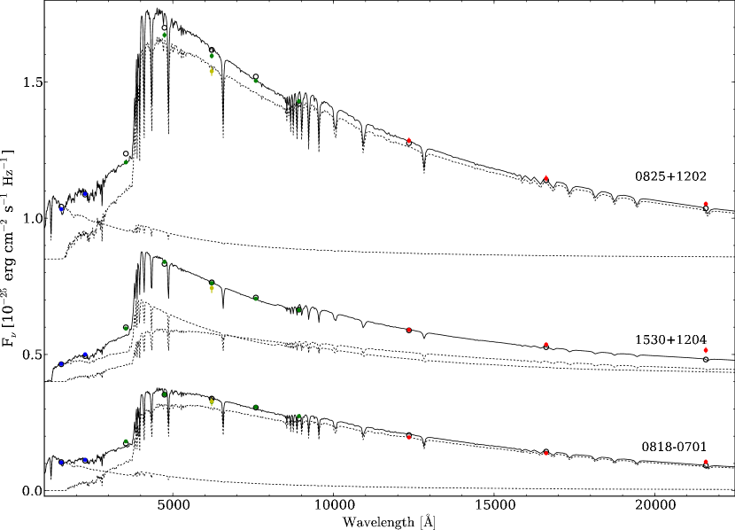
Figure 6: The SEDs of, and fits to, 0818$-$0701, 0825$+$1202 and 1530$+$1204, following the same format as Figure 5. The fit to 0818$-$0701 comprises a $\mbox{$\mathrm{T}_{\mathrm{eff}}$}=22,000$ K sdB model and a $7,750$ K star (black dashed lines). Similarly, a $\mbox{$\mathrm{T}_{\mathrm{eff}}$}=22,000$ K sdB model and a $8,250$ K star is used for 0825$+$1202 and a $\mbox{$\mathrm{T}_{\mathrm{eff}}$}=11,000$ K sdB model and a $8,000$ K star for 1530$+$1204. 1530$+$1204 and 0825$+$1202 are offset in flux by $0.40$ and $0.85$ units, respectively, for clarity.

7.1 Potential systematic temperature differences

When comparing the system parameters calculated herein and those from the literature, there are a number of possible causes for discrepancies: Firstly, one must consider the fact that often in the literature fitting is performed on the absorption line profiles of the subdwarf with a single star model (e.g. Saffer et al., 1994), whereas our study suggests that these systems all have a significant contribution from the companion. The single subdwarf fit would then result in biased system parameters.

Secondly, if the subdwarf’s companion is a sub-giant or giant type star, our method would underestimate the subdwarf’s effective temperature because we only use main–sequence star models for the companion. While this may affect isolated cases, we do not expect a significant population of sub-giant and giant companion stars to be present in our sample given the colour selection cuts we employed (see Section 4.2).

Finally, the suppression of the subdwarf’s ultraviolet flux due to line blanketing could cause a biased effective temperature. Subluminous B stars show peculiar abundance patterns. Some metals (mostly the lighter ones) are found to be strongly depleted, while heavier elements can be strongly enriched (O’Toole & Heber, 2006; Blanchette et al., 2008). The abundance patterns are caused by atomic diffusion, which depends on various parameters (see Michaud et al. 2011, for the state-of-the-art of modelling), however, metalicity may not be an important one. Because the abundance pattern differs from star to star, the ultraviolet line blocking for any individual subdwarf will deviate from that predicted from the solar metalicity models adopted here. Therefore, we cannot quantify the systematic uncertainty in the temperature determination of the subdwarf stars. O’Toole & Heber (2006) regard solar metalicity models as appropriate for sdB stars cooler than about $30000$ K, but prefer models of scaled supersolar abundances for hotter stars as a proxy for enhanced ultraviolet line blocking. Because the effective temperatures of our program stars are mostly below $30000$ K, we stay with solar metalicity model spectra.

7.2 0018$+$0101

Lisker et al. (2005) calculated an effective temperature for 0018$+$0101 (HE 0016$+$0044) of $28,264\pm 800$ K. This compares relatively well with our SU sample estimate of $25,000-23,000$ K, however, a significantly higher temperature is measured when using the C2MS sample ($39,000-40,000$ K). Either a $23,000$ or a $40,000$ K subdwarf provide an adequate fit to the SED, and small changes in the $\chi^{2}$ surface lead to the alternate solution. The flat $\chi^{2}$ surface comes about from a very blue $(\mbox{$\mathrm{m}_{\mathrm{FUV}}$}-\mbox{$\mathrm{m}_{\mathrm{NUV}}$})$ colour ($-0.64$) that is difficult to reconcile with the rest of the SED.

7.3 1300$+$0057 and 1538$+$0934

The published effective temperatures for 1300$+$0057 ($39359$ K: HE 1258$+$0113: Stroeer et al., 2007) and 1538$+$0934 ($35114$ K: HS 1536$+$0944: Lisker et al., 2005), both in the SU sample, are only upper limits on the effective temperatures. Lisker et al. (2005) note the presence of a cool ($\sim$K0-type) companion in the spectrum of 1538$+$0934 and therefore specifically state that the estimated temperature is an upper limit. Stroeer et al. (2007) also note the presence of a cool companion based on the $B-J$ colour for 1300$+$0057 and therefore one may assume the temperature is also an overestimate. In both cases, the best fit model ($30,000$ and $23,000$ K for 1300$+$0057 and 1538$+$0934, respectively) corresponds to a bluer $(\mbox{$\mathrm{m}_{\mathrm{FUV}}$}-\mbox{$\mathrm{m}_{\mathrm{NUV}}$})$ colour than the GALEX fluxes. Therefore using the higher published effective temperature model would not agree with the data.

7.4 1517$+$0310 and 1518$+$0410

In the case of 1517$+$0310 and 1518$+$0410 (PG 1514$+$034 and PG 1515$+$044, respectively: SU sample), the companion effective temperatures measured ($6,000\{^{6,250}_{5,750}$ K and $5,500\{^{5,750}_{5,250}$ K, respectively) are significantly different from that in the catalogue of Østensen (2006) (K2 and K4.5; corresponding to effective temperatures of $\sim 4,800$ and $4,300$ K, respectively). The whole SED of 1517$+$0310 is not particularly well fit by the calculated best model. The system has a very blue $(\mbox{$\mathrm{m}_{\mathrm{FUV}}$}-\mbox{$\mathrm{m}_{\mathrm{NUV}}$})$ colour and therefore the best fit model is forced to be a hot subdwarf, which leads to a correspondingly increased companion effective temperature.

7.5 1709$+$4054

1709$+$4054 (PG 1708$+$409: C2MS sample), was classified by Saffer et al. (1994) to be a subdwarf with an effective temperature of $28,500$ K. We determined $25,000-28,000$ K if we apply no reddening and $27,000-29,000$ K when applying the full Schlegel et al. (1998) reddening. However, Saffer et al. (1994) fit the line profiles of this composite system with a single star subdwarf model, and therefore comparing the two sets of temperatures is not comparing like for like.

7.6 2138$+$0442

For the case of 2138$+$0442 (PG 2135$+$045; C2MS sample), we find a slightly lower effective temperature ($24,000-26,000$ K) compared with the published value of Aznar Cuadrado & Jeffery ($\sim 28,000$ K: 2002). Including the full Schlegel et al. (1998) reddening ($26,000-28,000$ K), however, the temperatures agree. Aznar Cuadrado & Jeffery (2002) treat 2138$+$0442 as a composite system fitting both objects in the blue region of the spectrum, thus the above mentioned problem of fitting a single star model (Section 7.1) does not apply.

7.7 2244$+$0106

2244$+$0106 (PB 5146) was found to be a post-EHB star with a high velocity in Tillich et al. (Hyper-MUCHFUSS; 2011). They estimate a $\mbox{$\mathrm{T}_{\mathrm{eff}}$}=33580\pm 680$ K, $\mbox{$\log\,g$}=4.75\pm 0.20$ and a distance of $18.29\pm 2.45$ kpc, compared with our $22,000-26,000$ K at $6.1-7.9$ kpc. However, the companion star is not accounted for in Tillich et al. (2011) and therefore the subdwarfs effective temperature is probably overestimated. This is also consistent with the unusually low surface gravity.

7.8 Overlap

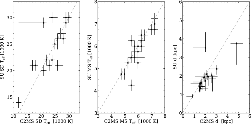
Figure 7: A comparison of fits using the C2MS sample versus that using the SU sample, where there is overlap. Objects with a “Q”$\geq 3$ in Table 7 are excluded. The dashed line shows a one to one relation between the parameters.

Where the C2MS and SU samples overlap, a comparison of the fits is given in Table 7 and shown in Figure 7. The two sets of fits appear consistent within the uncertainties. We analysed the distribution of the difference between all the C2MS and SU parameters (distance, subdwarf and companion temperature) and find that the distributions are all approximately Gaussian, centered about zero. We do not find any evidence to suggest that the two samples effective temperatures are systematically offset. The errors on the subdwarf effective temperature from the $\chi^{2}$ fit may be slightly underestimated, and a more realistic error is a few thousand Kelvin. The one difference is that the UKIDSS data should better constrain the companion star effective temperature due to the greater depth and higher photometric accuracy of the near-infrared data.

Overall, in individual cases, we must bear in mind that we may occasionally select the wrong solution (in cases where the $\chi^{2}$ surface is relatively flat), nor can we identify the exact amount of reddening that should be corrected for. However, this study is aimed at providing a statistical analysis of the sample rather than correct parameters for all individual systems. The errors in the measured parameters should be randomly distributed and therefore not effect the distributions. It is thus not a significant issue for the analysis presented here, but these uncertainties should be considered when consulting the fitted parameters of individual systems.

We saw earlier that the key contaminants in our colour box are composite systems containing white dwarfs (Table 3). Indeed, from the C2MS sample 0018$+$0101, 0141$+$0614, 0923$+$0652, 2117$-$0015 and 2117$-$0006 are candidates for being DA white dwarfs with infrared excesses based on their photometry (Girven et al., 2011). However, such a classification can only be confirmed through follow-up spectroscopy. SDSS spectroscopy is available for 2117$-$0006, and Girven et al. (2011) classify it as a “Narrow Line Hot Star” (NLHS), which they believe to be a group primarily made up of subdwarfs. 0018$+$0101, discussed in Section 7.2, is also catalogued as a NLHS by Girven et al. (2011), corroborating the subdwarf label.

Table 5: Individual objects of interest from the C2MS sample. Only subdwarfs with measured system parameters are displayed, but all known CVs and white dwarfs are shown. The “{” notation is described in Section 7 and does not simply represent uncertainties. The fit parameters shown are not corrected for interstellar reddening. The comments quoted for the possible white dwarfs matched in Girven et al. (2011) are the classifications according to the SDSS spectra found therein. NLHS corresponds to Narrow Line Hot Star (probable subdwarf).

			This Paper			Literature
Name	Identifier	sdB $\mathrm{T}_{\mathrm{eff}}$	MS $\mathrm{T}_{\mathrm{eff}}$	d	sdB $\mathrm{T}_{\mathrm{eff}}$	MS Type	Ref / Comments
		(1000K)	(1000K)	(kpc)	(K)
Subdwarfs
0018$+$0101	HE 0016$+$0044	$40\{^{40}_{39}$	$5.50\{^{5.75}_{5.25}$	$1.5\{^{1.5}_{1.4}$	28264		Lisker et al. (2005)
1212$+$4240	PG 1210$+$429	$23\{^{24}_{22}$	$5.75\{^{6.00}_{5.50}$	$1.5\{^{1.7}_{1.4}$		K2.5	Østensen (2006)
1517$+$0310	PG 1514$+$034	$40\{^{40}_{39}$	$6.00\{^{6.25}_{5.75}$	$1.1\{^{1.1}_{1.0}$		K2	Østensen (2006)
1709$+$4054	PG 1708$+$409	$26\{^{28}_{25}$	$5.50\{^{5.75}_{5.25}$	$1.7\{^{1.9}_{1.6}$	28500		Saffer et al. (1994, 1998)
2138$+$0442	PG 2135$+$045	$25\{^{26}_{24}$	$5.00\{^{5.25}_{4.75}$	$1.2\{^{1.3}_{1.1}$	$\sim 28000$	$\sim$K2	Aznar Cuadrado & Jeffery (2002)
CV
0141$+$0614	HS 0139$+$0559	$12\{^{13}_{11}$	$7.25\{^{7.50}_{7.00}$	$4.8\{^{5.4}_{4.3}$			Heber et al. (1991),
							Aungwerojwit et al. (2005)
0812$+$1911		$14\{^{15}_{13}$	$7.25\{^{7.50}_{7.00}$	$4.8\{^{6.9}_{4.8}$			Szkody et al. (2006)
1015$-$0308	SW Sex	$18\{^{19}_{17}$	$7.00\{^{7.25}_{6.75}$	$2.6\{^{2.9}_{2.3}$			e.g. Green et al. (1982),
							Penning et al. (1984)
2143$+$1244		$30\{^{31}_{29}$	$6.25\{^{6.50}_{6.00}$	$2.9\{^{3.3}_{2.6}$			Szkody et al. (2005)
Possible WD							Girven et al. (2011)
0018$+$0101	HS 0016$+$0044	$40\{^{40}_{39}$	$5.50\{^{5.75}_{5.25}$	$1.5\{^{1.5}_{1.4}$			NLHS
0141$+$0614	HS 0139$+$0559	$12\{^{13}_{11}$	$7.25\{^{7.50}_{7.00}$	$4.8\{^{5.4}_{4.3}$
0923$+$0652		$29\{^{30}_{28}$	$6.75\{^{7.00}_{6.50}$	$2.1\{^{2.9}_{2.0}$
2117$-$0015		$13\{^{14}_{12}$	$6.75\{^{7.00}_{6.50}$	$3.5\{^{3.5}_{2.3}$
2117$-$0006		$21\{^{22}_{20}$	$6.25\{^{6.50}_{6.00}$	$2.0\{^{2.9}_{1.9}$			NLHS

Table 6: Individual objects of interest from the SU sample. The “{” notation is described in Section 7 and does not simply represent uncertainties. The comments quoted for the possible white dwarfs matched in Girven et al. (2011) are the classifications according to the SDSS spectra found therein. DA and NLHS correspond to DA white dwarf and Narrow Line Hot Star (probable subdwarf), respectively.

			This Paper			Literature
Name	Identifier	sdB $\mathrm{T}_{\mathrm{eff}}$	MS $\mathrm{T}_{\mathrm{eff}}$	d	sdB $\mathrm{T}_{\mathrm{eff}}$	MS Type	Ref / Comments
		(1000K)	(1000K)	(kpc)	(K)
Subdwarfs
0018$+$0101	HE 0016$+$0044	$24\{^{25}_{23}$	$4.25\{^{4.50}_{4.00}$	$1.2\{^{1.3}_{1.2}$	28264		Lisker et al. (2005)
1300$+$0057	HE 1258$+$0113	$30\{^{31}_{29}$	$3.50\{^{3.75}_{3.25}$	$1.7\{^{1.8}_{1.6}$	39359a		Stroeer et al. (2007)
1517$+$0310	PG 1514$+$034	$40\{^{40}_{39}$	$6.00\{^{6.25}_{5.75}$	$1.1\{^{1.2}_{1.0}$		K2	Østensen (2006)
1518$+$0410	PG 1515$+$044	$26\{^{27}_{25}$	$5.50\{^{5.75}_{5.25}$	$1.8\{^{2.0}_{1.7}$		K4.5	Østensen (2006)
1538$+$0934	HS 1536$+$0944	$23\{^{24}_{22}$	$5.00\{^{5.25}_{4.75}$	$1.8\{^{2.0}_{1.7}$	35114a	K0	Lisker et al. (2005)
CV
0141$+$0614	HS 0139$+$0559	$14\{^{15}_{13}$	$7.25\{^{7.50}_{7.00}$	$3.7\{^{4.9}_{3.7}$			Heber et al. (1991)
0813$+$2813		$20\{^{21}_{19}$	$6.25\{^{6.50}_{6.00}$	$6.4\{^{6.7}_{4.6}$			Szkody et al. (2005)
0920$+$3356	BK Lyn	$20\{^{21}_{18}$	$6.75\{^{7.00}_{6.25}$	$2.3\{^{2.3}_{1.7}$			Dobrzycka & Howell (1992),
							Ringwald (1993)
1015$-$0308	SW Sex	$21\{^{22}_{20}$	$6.75\{^{7.00}_{6.50}$	$2.0\{^{2.5}_{1.9}$			e.g. Ballouz & Sion (2009),
							Ritter & Kolb (2009)
2333$+$1522		$17\{^{18}_{16}$	$6.75\{^{7.00}_{6.50}$	$12.6\{^{17.8}_{12.3}$			Szkody et al. (2005)
WDMS							Rebassa-Mansergas et al. (2011)
0032$+$0739		$21\{^{22}_{20}$	$5.25\{^{5.50}_{5.00}$	$4.4\{^{6.9}_{4.4}$
0300$-$0023	WD 0257$-$005	$38\{^{39}_{34}$	$5.00\{^{5.25}_{4.75}$	$3.2\{^{3.4}_{2.8}$
0920$+$1057		$34\{^{35}_{33}$	$4.75\{^{5.00}_{4.50}$	$3.3\{^{3.5}_{3.1}$
1016$+$0443		$29\{^{30}_{28}$	$4.50\{^{4.75}_{4.25}$	$4.8\{^{7.9}_{4.8}$
1352$+$0910		$29\{^{30}_{28}$	$4.00\{^{4.25}_{3.75}$	$4.0\{^{6.5}_{4.0}$
Possible WD							Girven et al. (2011)
0018$+$0101	HS 0016$+$0044	$24\{^{25}_{23}$	$4.25\{^{4.50}_{4.00}$	$1.2\{^{1.3}_{1.2}$			NLHS
0032$+$0739		$21\{^{22}_{20}$	$5.25\{^{5.50}_{5.00}$	$4.4\{^{6.9}_{4.4}$			DA
0141$+$0614	HS 0139$+$0559	$14\{^{15}_{13}$	$7.25\{^{7.50}_{7.00}$	$3.7\{^{4.9}_{3.7}$
0814$+$2811		$22\{^{23}_{21}$	$6.00\{^{6.25}_{5.75}$	$3.7\{^{4.0}_{3.3}$			NLHS
0854$+$0853	PN A66 31	$40\{^{40}_{39}$	$3.00\{^{3.25}_{3.00}$	$1.2\{^{1.2}_{1.2}$
0920$+$3356	BK Lyn	$20\{^{21}_{18}$	$6.75\{^{7.00}_{6.25}$	$2.3\{^{2.3}_{1.7}$
0925$-$0140		$17\{^{18}_{16}$	$5.50\{^{5.75}_{5.25}$	$9.4\{^{14.9}_{9.4}$
0951$+$0347		$23\{^{24}_{22}$	$4.00\{^{4.25}_{3.75}$	$1.9\{^{2.0}_{1.7}$			NLHS
0959$+$0330	PG 0957$+$037	$31\{^{32}_{30}$	$3.00\{^{3.25}_{3.00}$	$1.1\{^{1.2}_{1.1}$
1006$+$0032	PG 1004$+$008	$26\{^{27}_{25}$	$5.00\{^{5.25}_{4.75}$	$3.3\{^{3.6}_{3.1}$
1100$+$0346		$34\{^{36}_{33}$	$3.75\{^{4.25}_{3.50}$	$2.7\{^{2.9}_{2.6}$			NLHS
1116$+$0755		$28\{^{29}_{27}$	$5.00\{^{5.25}_{4.75}$	$2.3\{^{2.3}_{1.4}$
1135$+$0731		$29\{^{30}_{28}$	$6.25\{^{6.50}_{6.00}$	$6.4\{^{8.2}_{5.7}$			NLHS
1215$+$1351		$21\{^{22}_{20}$	$4.50\{^{4.75}_{4.25}$	$3.1\{^{5.1}_{3.1}$			NLHS
1228$+$1040	WD 1226$+$110	$21\{^{22}_{20}$	$3.00\{^{3.25}_{3.00}$	$2.2\{^{3.8}_{2.2}$			DA: Gänsicke et al. (2006)
1237$-$0151		$23\{^{25}_{22}$	$4.75\{^{5.00}_{4.50}$	$3.9\{^{4.3}_{3.6}$
1300$+$0057	HE 1258$+$0113	$30\{^{31}_{29}$	$3.50\{^{3.75}_{3.25}$	$1.7\{^{1.8}_{1.6}$			NLHS
1315$+$0245		$33\{^{34}_{32}$	$3.25\{^{3.50}_{3.00}$	$0.9\{^{1.0}_{0.8}$
1323$+$2615		$20\{^{21}_{19}$	$5.00\{^{5.25}_{4.75}$	$5.8\{^{5.8}_{3.6}$
1352$+$0910		$29\{^{30}_{28}$	$4.00\{^{4.25}_{3.75}$	$4.0\{^{6.5}_{4.0}$			DA
1422$+$0920		$26\{^{27}_{25}$	$4.75\{^{5.00}_{4.50}$	$3.5\{^{3.7}_{3.2}$			NLHS
1442$+$0910		$26\{^{27}_{24}$	$5.00\{^{5.25}_{4.75}$	$6.6\{^{7.1}_{5.9}$
1443$+$0931		$28\{^{29}_{27}$	$4.50\{^{4.75}_{4.25}$	$4.5\{^{4.5}_{2.7}$			NLHS
1500$+$0642		$27\{^{28}_{26}$	$4.25\{^{4.50}_{3.75}$	$3.9\{^{4.2}_{3.7}$			NLHS
1507$+$0724		$27\{^{28}_{26}$	$4.50\{^{4.75}_{4.25}$	$4.1\{^{4.4}_{3.8}$
1510$+$0409		$26\{^{27}_{25}$	$4.00\{^{4.25}_{3.75}$	$3.4\{^{3.6}_{3.2}$			NLHS
1525$+$0958		$29\{^{30}_{28}$	$3.25\{^{4.25}_{3.00}$	$2.8\{^{4.8}_{2.8}$			NLHS
1538$+$0644	HS 1536$+$0944	$14\{^{15}_{13}$	$7.25\{^{7.50}_{7.00}$	$6.5\{^{8.6}_{6.4}$
1543$+$0012	WD 1541$+$003	$21\{^{22}_{20}$	$4.75\{^{5.00}_{4.50}$	$2.9\{^{4.5}_{2.8}$			NLHS
1554$+$0616		$29\{^{30}_{28}$	$4.75\{^{5.00}_{4.50}$	$3.8\{^{5.8}_{3.6}$
1619$+$2407		$24\{^{25}_{23}$	$6.50\{^{6.75}_{6.25}$	$4.3\{^{4.8}_{3.8}$			NLHS
2049$-$0001		$18\{^{19}_{17}$	$5.25\{^{5.50}_{5.00}$	$6.0\{^{6.4}_{5.6}$
2117$-$0006		$30\{^{31}_{29}$	$6.50\{^{6.75}_{6.25}$	$2.1\{^{2.3}_{1.8}$			NLHS
2147$-$0112	FBS 2145$-$014	$25\{^{26}_{24}$	$3.25\{^{3.50}_{3.00}$	$1.6\{^{1.7}_{1.5}$

^a Noted presence of a cool companion, therefore temperature is an upper limit, see Section 7.3.

Table 7: Comparison of fits using the C2MS sample against that using the SU sample where there is overlap. The “{” notation is described in Section 7 and does not simply represent uncertainties. The “Q” (Quality) column values correspond to; 1:Good fit, 2:Average fit, 3:Poor fit, 4:WD/WD+MS/CV and 5:Quasar/Galaxy.

		C2MS				SU
		sdB $\mathrm{T}_{\mathrm{eff}}$	MS $\mathrm{T}_{\mathrm{eff}}$	d	Q	sdB $\mathrm{T}_{\mathrm{eff}}$	MS $\mathrm{T}_{\mathrm{eff}}$	d	Q
Name	Identifier	(1000K)	(1000K)	(kpc)		(1000K)	(1000K)	(kpc)
0018+0101	HE 0016$+$0044	$40\{^{40}_{39}$	$5.50\{^{5.75}_{5.25}$	$1.5\{^{1.5}_{1.4}$	2	$24\{^{25}_{23}$	$4.25\{^{4.50}_{4.00}$	$1.2\{^{1.3}_{1.2}$	1
0054+1508		$21\{^{22}_{20}$	$7.25\{^{7.50}_{7.00}$	$3.2\{^{4.8}_{3.2}$	2	$29\{^{30}_{28}$	$7.25\{^{7.50}_{7.00}$	$2.8\{^{3.3}_{2.7}$	3
0141+0614	HS 0139$+$0559	$12\{^{13}_{11}$	$7.25\{^{7.50}_{7.00}$	$4.8\{^{5.4}_{4.3}$	1	$14\{^{15}_{13}$	$7.25\{^{7.50}_{7.00}$	$3.7\{^{4.9}_{3.7}$	2
0316+0042	PG 0313$+$005	$28\{^{29}_{27}$	$6.25\{^{6.50}_{6.00}$	$2.2\{^{2.2}_{1.4}$	1	$26\{^{27}_{25}$	$6.00\{^{6.25}_{5.75}$	$2.0\{^{2.2}_{1.8}$	1
0737+2642		$25\{^{26}_{24}$	$5.50\{^{5.75}_{5.25}$	$1.6\{^{1.8}_{1.5}$	1	$25\{^{26}_{24}$	$5.50\{^{5.75}_{5.25}$	$1.6\{^{1.8}_{1.5}$	1
0755+2128		$17\{^{18}_{16}$	$7.25\{^{7.50}_{7.00}$	$2.3\{^{3.5}_{2.3}$	1	$21\{^{22}_{20}$	$7.00\{^{7.25}_{6.75}$	$2.0\{^{2.4}_{1.9}$	1
0814+2019		$21\{^{22}_{20}$	$5.50\{^{5.75}_{5.25}$	$2.0\{^{3.2}_{2.0}$	1	$20\{^{21}_{19}$	$6.25\{^{6.50}_{6.00}$	$3.5\{^{3.7}_{2.7}$	1
0829+2246		$26\{^{27}_{24}$	$6.00\{^{6.25}_{5.75}$	$2.7\{^{3.0}_{2.4}$	1	$21\{^{22}_{20}$	$5.25\{^{5.50}_{5.00}$	$1.9\{^{2.6}_{1.8}$	1
0833-0006		$29\{^{30}_{28}$	$7.25\{^{7.50}_{7.00}$	$3.1\{^{3.6}_{2.9}$	2	$29\{^{30}_{28}$	$6.75\{^{7.00}_{6.50}$	$2.4\{^{2.7}_{2.1}$	2
0929+0603		$21\{^{30}_{20}$	$5.75\{^{6.00}_{5.50}$	$1.6\{^{2.5}_{1.5}$	2	$29\{^{30}_{28}$	$6.00\{^{6.25}_{5.75}$	$1.6\{^{2.0}_{1.4}$	1
0937+0813	PG 0935$+$084	$23\{^{24}_{22}$	$6.00\{^{6.25}_{5.75}$	$2.0\{^{2.3}_{1.8}$	1	$21\{^{22}_{20}$	$5.75\{^{6.00}_{5.50}$	$1.7\{^{2.3}_{1.6}$	1
0941+0657	PG 0939$+$072	$21\{^{22}_{20}$	$6.25\{^{6.50}_{6.00}$	$1.7\{^{2.5}_{1.6}$	1	$29\{^{30}_{28}$	$6.50\{^{6.75}_{6.25}$	$1.7\{^{2.0}_{1.5}$	2
1015-0308	SW Sex	$18\{^{19}_{17}$	$7.00\{^{7.25}_{6.75}$	$2.6\{^{2.9}_{2.3}$	1	$21\{^{22}_{20}$	$6.75\{^{7.00}_{6.50}$	$2.0\{^{2.5}_{1.9}$	2
1018+0953		$28\{^{29}_{27}$	$5.75\{^{6.00}_{5.00}$	$1.6\{^{1.6}_{1.0}$	1	$35\{^{36}_{34}$	$5.50\{^{5.75}_{5.25}$	$1.3\{^{1.5}_{1.2}$	1
1113+0413	PG 1110$+$045	$29\{^{30}_{28}$	$4.75\{^{5.00}_{4.50}$	$0.9\{^{1.4}_{0.9}$	1	$30\{^{31}_{29}$	$4.75\{^{5.00}_{4.50}$	$0.9\{^{1.0}_{0.8}$	1
1203+0909	PG 1200$+$094	$27\{^{28}_{25}$	$5.75\{^{6.00}_{5.50}$	$1.5\{^{1.6}_{1.3}$	1	$27\{^{28}_{26}$	$5.75\{^{6.00}_{5.50}$	$1.5\{^{1.6}_{1.3}$	1
1233+0834		$30\{^{31}_{29}$	$6.00\{^{6.25}_{5.75}$	$1.9\{^{2.1}_{1.7}$	2	$30\{^{31}_{29}$	$6.00\{^{6.25}_{5.75}$	$1.9\{^{2.2}_{1.7}$	1
1325+1212	PG 1323$+$125	$26\{^{27}_{25}$	$5.75\{^{6.00}_{5.50}$	$2.1\{^{2.3}_{1.9}$	1	$26\{^{28}_{25}$	$5.75\{^{6.00}_{5.50}$	$2.1\{^{2.4}_{1.9}$	1
1326+0357	PG 1323$+$042	$24\{^{25}_{23}$	$5.00\{^{5.25}_{4.75}$	$1.5\{^{1.7}_{1.4}$	2	$22\{^{23}_{21}$	$4.75\{^{5.00}_{4.50}$	$1.4\{^{1.5}_{1.2}$	1
1402+3215		$22\{^{23}_{21}$	$6.25\{^{6.50}_{6.00}$	$1.9\{^{2.1}_{1.7}$	1	$22\{^{23}_{21}$	$6.25\{^{6.50}_{6.00}$	$1.9\{^{2.1}_{1.7}$	1
1421+0753	KN Boo	$27\{^{28}_{26}$	$5.25\{^{5.50}_{5.00}$	$1.6\{^{1.7}_{1.5}$	1	$27\{^{28}_{26}$	$5.25\{^{5.50}_{5.00}$	$1.6\{^{1.7}_{1.5}$	1
1502-0245	PG 1459$-$026	$24\{^{25}_{22}$	$6.25\{^{6.50}_{6.00}$	$1.8\{^{1.9}_{1.5}$	1	$30\{^{31}_{29}$	$6.00\{^{6.25}_{5.75}$	$1.4\{^{1.6}_{1.3}$	1
1542+0056		$29\{^{30}_{28}$	$6.50\{^{6.75}_{6.25}$	$1.5\{^{2.1}_{1.4}$	1	$29\{^{30}_{28}$	$6.50\{^{6.75}_{6.25}$	$1.5\{^{1.7}_{1.3}$	1

7.9 Distributions of fits – C2MS sample

The distribution of subdwarf and companion effective temperatures for the C2MS sample is shown in Figure 8 and the distribution of distances for the C2MS and SU samples in Figure 9. Here we compare the parameters with and without reddening corrections. Objects that are known to be contaminants, such as white dwarfs and CVs, have been removed from all three (distance, subdwarf and companion temperature) histograms. For galaxies, these should be flagged by SDSS and are therefore removed by the flags in Table 1. Using Table 3 to estimate the remaining fraction of contaminants, we know that $12$ per cent ($3/25$) of the objects with SDSS spectra are contaminants. Therefore, approximately eleven ($12$ per cent of $93$) of the whole C2MS sample will be contaminants. The two CVs and one white dwarf with SDSS spectra (Table 3) can be removed from the histograms. Thus, the contamination of the C2MS sample (now with and without SDSS spectra) used for calculating distributions will be $9$ per cent ($8/90$). Since any such contaminants will be distributed right across our fit parameters, we believe they do not distort our statistical analysis to a significant degree.

7.9.1 Subdwarf temperature distribution

Taking the system parameters calculated without correcting for reddening, we find that the subdwarf effective temperatures (Figure 8) are spread from $20,000-30,000$ K and peak in the $20,000-24,000$ K range. We do see a pronounced drop in numbers below $20,000$ K. Reddening is not the issue here; applying the full Schlegel et al. (1998) reddening correction to the objects before fitting does not lead to a significant shift in the distribution, though it is slightly smoothed.

Based on our theoretical tracks for composite systems, we know that we have a reduced completeness below $\sim 25,000$ K (see Section 4.2). For example, cool subdwarfs of $\sim 15,000$ K with an M-type companion will be missed by the colour selection. This could lead to a bias towards hotter subdwarfs, which we select over a wider range of companion types. In addition, the redder $(\mbox{$r_{\mathrm{CMC}}$}-K_{s})$ colours (Figure 2) means that at the $K_{s}$ magnitude limit ($14.3$), systems will be detected down to fainter $r_{\mathrm{CMC}}$ magnitudes. This is however offset by the increasing intrinsic brightness of cooler subdwarfs (because of decreasing $\log\,g$ and increasing radius). We previously discussed a bias towards cooler subdwarfs if our assumption of a main–sequence type companion is incorrect (Section 7.1). However, we believe this to be a relatively small fraction given our sample selection (Section 4.2).

To quantify these possible biases, the limitations on distance introduced by various magnitude cuts can be seen in Table 8. These are derived by taking the absolute magnitudes of the composite system and calculating the distance the object would have to be moved to in order to have an apparent magnitude at the relevant limit. The primary effects in this case are caused by the saturation limit of SDSS ($\mbox{$r_{\mathrm{SDSS}}$}>14.1$), corresponding to a minimum distance, and the faint $K_{s}$ magnitude limit of 2MASS ($K_{s}<14.3$), setting a maximum distance. These significantly depend on companion spectral type (see below) and, to a lesser extent, on subdwarf effective temperature. It can be seen that the imposed $r_{\mathrm{CMC}}$ magnitude limit does not have an effect because the $K_{s}$ limit is always more restrictive. In essence, in the C2MS sample, the 2MASS depth limits the volume over which we are reasonably complete.

7.9.2 Companion type distribution

As discussed in Section 4.2, the way in which we select subdwarfs with companions introduces a bias in companion type. We expect our selection to be complete for subdwarfs with $20,000\leq\mbox{$\mathrm{T}_{\mathrm{eff}}$}\leq 35,000$ K and companions in the range A5 to M5-type. Similarly, including the more extreme subdwarf temperatures ($15,000\leq\mbox{$\mathrm{T}_{\mathrm{eff}}$}\leq 40,000$ K), we are complete for F0 to K0-type companions. The companion type range is smaller in the latter case because, for example, a $40,000$ K subdwarf with a M5-type companion does not fall in our colour selection, whereas a $35,000$ K subdwarf with a M5-type companion does.

The distribution of companion effective temperature in Figure 8 ramps up from early spectral types towards $\sim$ G0, as might be expected from the initial mass function (IMF). On the other hand, the subsequent turn over and drop towards mid-K-type may be a product of our selection biases. A $15,000$ K subdwarf with a M0-type companion saturates in SDSS at $d\leq 1.7$ kpc and is too faint for 2MASS at $d\geq 1.7$ kpc (Table 8). Therefore we are not sensitive to all subdwarfs with M0-type companions. The best way to reduce such biases and test our completion is by probing to fainter $K_{s}$-band magnitudes. This was the key motivation behind our second sample, using SU which extends several magnitudes deeper and reaches $K\sim 17.8$, though at the expense of limited sky coverage.

Table 8: Limitations on the distance of subdwarf plus main–sequence star candidates caused by the relative magnitude cuts. This is calculated for $15,000$, $20,000$, $30,000$ and $40,000$ K subdwarfs and companions with effective temperatures of $3,250$ K (M0), $5,000$ K (K0), $7,250$ K (F0). The important limits considered are; the saturation of $r_{\mathrm{SDSS}}$ at 14.1 (therefore a minimum distance), the cut made on $r_{\mathrm{CMC}}$ at 16.0 (therefore a maximum distance), the $K_{s}$-band magnitude limit of 2MASS at 14.3 and the $K_{s}$-band magnitude limit of UKIDSS at 17.8.

sdB $\mathrm{T}_{\mathrm{eff}}$	MS $\mathrm{T}_{\mathrm{eff}}$	Abs	d (kpc)		Abs	d (kpc)
(K)	(K)	$r$	$r_{\mathrm{SDSS}}$=14.1	$r_{\mathrm{CMC}}$=16.0	$K$	$Ks$=14.3	$K$=17.8
$15,000$	$7,250$	2.2	2.4	5.8	1.9	3.1	15.6
	$5,000$	2.9	1.7	4.1	2.8	2.0	9.9
	$3,250$	3.0	1.7	4.0	3.2	1.7	8.5
$20,000$	$7,250$	2.5	2.1	5.0	2.0	2.8	14.3
	$5,000$	3.6	1.3	3.0	3.4	1.5	7.7
	$3,250$	3.7	1.2	2.8	4.0	1.1	5.8
$30,000$	$7,250$	2.8	1.8	4.4	2.2	2.7	13.5
	$5,000$	5.0	0.7	1.6	3.9	1.2	6.0
	$3,250$	5.5	0.5	1.2	5.3	0.6	3.1
$40,000$	$7,250$	2.7	1.9	4.5	2.2	2.7	13.5
	$5,000$	4.6	0.8	1.9	3.9	1.2	6.2
	$3,250$	5.0	0.7	1.6	5.1	0.7	3.5

7.9.3 Distance distribution

The calculated distance distribution seen in Figure 9 shows a rapid increase towards $\sim 2$kpc, followed by an extended tail. As we discussed previously, the limitations on distance due to our magnitude cuts and limits are important and are a complex function of subdwarf effective temperature and companion type (Table 8). There are no clean regions where all temperatures and companion types are sampled evenly to give a complete, volume-limited sample. If one assumes that all subdwarfs (independent of temperature and companion type) are drawn from same parent distance distribution, and we select each subdwarf–companion system with equal probability, the distribution shown in Figure 9 would represent the true distance distribution. Therefore we would be relatively confident that the peak appears at $1.5-2.0$kpc. However, Table 8 does show that for some combinations of subdwarf and companion temperature we are no longer complete at this peak distance. Here again the deeper SU sample can provide us with a more complete sample.

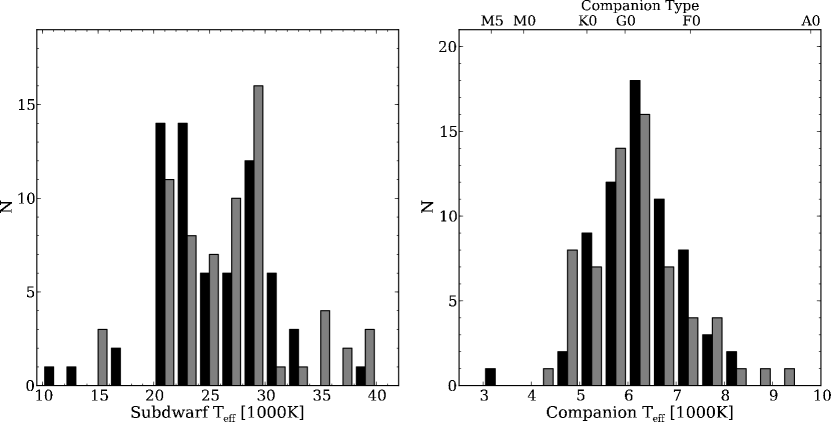
Figure 8: Distributions of the subdwarf (left) and companion (right) effective temperatures calculated from the fitting method described in Section 6 when applied to the C2MS sample. The grey and black histograms show the system parameters when calculated with and without the (maximum) reddening correction, respectively. Adjoining pairs of histogram show the number of objects in the same bin. A total of 66 objects are included in the histograms, where 27 objects that are known to be contaminants (from their SIMBAD classification or their SDSS spectra), or the subdwarf–companion model provides a bad fit (“Q”$\geq 3$ in Table 10), have been removed. The subdwarf effective temperature histogram is grouped in bins of $2,000$ K and the companion star histogram uses bins of $500$ K.

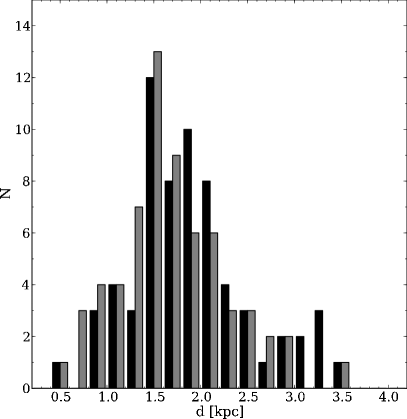
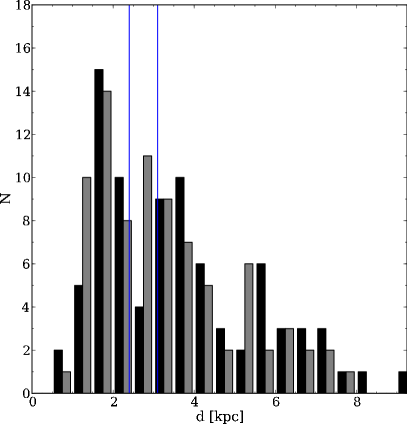
Figure 9: Distribution of the distance to the subdwarf-companion star systems as calculated from the fitting method described in Section 6 when applied to the C2MS (left) and SU samples (right). The grey and black histograms show the system parameters when calculated with and without the reddening correction, respectively. Adjoining pairs of histogram show the number of objects in the same bin. Objects that are known to be contaminants have been removed. A total of 66 objects are included in the C2MS histogram (left), where 27 objects that are known to be contaminants (from their SIMBAD classification or their SDSS spectra), or the subdwarf–companion model provides a bad fit (“Q”$\geq 3$ in Table 10 or 13), have been removed. In the SU histogram, 84 objects are included, where 50 have been removed. The distances are given in kpc and the bin sizes are $0.2$ and $0.5$ kpc for the C2MS and SU samples, respectively. The vertical lines in the right hand plot show the region where the volume limit sample is defined ($2.4$ to $3.1$ kpc).

7.10 Distribution of fits – SU sample

The corresponding distributions of the subdwarf and companion effective temperature for the SU sample are shown in Figure 10 with the distribution of distances in Figure 9. The subdwarf effective temperature distribution is broadly consistent with that of the C2MS sample, with most subdwarf temperatures between $20,000-30,000$ K. It is also similar to that shown for uncontaminated sdBs by Green et al. (2006, Figure 1). To establish a volume–limited sample, we again refer to Table 8 where we contrast the impact of the 2MASS versus UKIDSS $K$-band limits. The distances sampled are significantly larger, though as before dependent on subdwarf and companion temperature. Overall, the SU sample should be less biased against finding lower temperature subdwarfs compared to the C2MS sample (see the second example given in Section 7.9.2; a $15,000$ K subdwarf with a M0-type companion would now be detected to $8.5$ kpc). This does not appear to have increased the numbers of low temperature subdwarfs found and thus it appears that their absence is not due to our sample biases, but represents an intrinsic deficit of cool subdwarfs within the subdwarf population. Accounting for reddening (as seen in the grey histogram) does not have a large effect, although it shifts the calculated subdwarf effective temperatures systematically higher by $1,000-2,000$ K.

Comparing the distribution of companion effective temperatures to the C2MS sample, the SU sample has a larger number of objects with early M-type companions. Hence, the SU sample overcomes the main limitation found within the C2MS sample, the shallow $K_{s}$-band data. The increased depth of UKIDSS allows us to probe significantly more systems with M-type companions, however we still see a deficit compared with K-type companions and earlier. This also seems obvious from the lack of systems populating the subdwarf plus M-type companion region of the colour-colour diagram in Figure 1. Selecting subdwarfs with companions later than $\sim$M5-type is still limited by the colour selection method as discussed previously (Section 4.2). Probing deeper in the $K$-band does not help for companion types later than $\sim$M5. Accounting for reddening has a complementary effect to that on effective temperature. As the subdwarfs become hotter, the required companion also shifts to higher temperatures.

We searched for a correlation between subdwarf and companion effective temperatures, but none was found at a level above the parameter uncertainties. Better statistics, from larger samples, are needed to investigate the subtleties of population.

Overall, when considering confirmed subdwarf systems, we believe that the fitting method is producing temperatures accurate to within a few thousand Kelvin and companion temperatures to within several hundred Kelvin (a few spectral types). There is some disagreement between individual fit results when compared with the literature. However, our principal goal is not to achieve superior parameters for individual systems. Indeed, more data are required to accurately establish parameters for individual systems. Our method does appear to be efficient in finding composite subdwarf binaries, while our SED fitting is accurate enough to allow us to consider the broad statistical parameter distributions within our samples. There will be some influence from contaminants. However, the numbers of contaminants are a relatively small fraction (Table 3) and wherever possible they have been removed from the distributions.

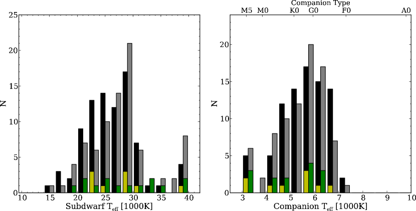
Figure 10: Distributions of the subdwarf (left) and companion (right) effective temperatures calculated from the fitting method described in Section 6 when applied to the SU sample. The grey and black histograms show the system parameters when calculated with and without the reddening correction, respectively. Adjoining pairs of histogram bars show the number of objects in the same bin. A total of 84 objects are included in the histograms, where 50 objects that are known to be contaminants (from their SIMBAD classification or their SDSS spectra), or the subdwarf–companion model provides a bad fit (“Q”$\geq 3$ in Table 10), have been removed. Similarly, the green and yellow histograms shows distributions (with and without reddening corrections) when the distances to the objects are limited to be between $2.4$ and $3.1$kpc, such that the histogram is a volume limited sample. 11 and 16 objects are included in the histograms, respectively. The subdwarf effective temperature histogram is grouped in bins of $2,000$ K and the companion star histogram uses bins of $500$ K.

7.11 A volume-limited sample

The advantage of using the SU sample is that significantly larger distances are probed. Referring to Table 8, the sample is complete for F0 to M0-type companions over distances of $2.4$ to $3.1$kpc. Although we can therefore construct a volume limited sample in this region, only 14 objects with good quality fits to the SED fall within this region (Figure 10). It is impossible to draw meaningful conclusions about parameter distributions for such a small sample.

Following the assumptions described in Section 7.9.3, and thus assuming the distribution seen in Figure 10 is representative of the true distance distribution, the peak at $2\pm 1$kpc in our distance distribution may then be associated with representing the spatial distribution of the bulk of the subdwarf binaries. Then, assuming the distribution follows a simple disk population of the form $r^{2}\mathrm{exp}(-r/H)$, where $r$ is the distance from the center of the disk and $H$ is the scale height, the turning point in a distance histogram should represent $2H$. Therefore, the scale height of the subdwarf population in the SU sample is $1\pm 0.5$kpc.

8 Discussion

Existing samples of subdwarfs have shown that a substantial fraction of them reside in binaries. Han et al. (2003) used population synthesis models to calculate that the intrinsic binary fraction should be $76-89$ per cent. Our samples explicitly target composite systems and thus should be dominated by subdwarfs with bound binary companions. Heber (2009) states that the vast majority of subdwarfs have a temperature between $20,000-40,000$ K. The temperature distribution found here appears approximately consistent with this range, however we do find a sub-sample of cooler subdwarfs with temperatures below $20,000$ K. In the SU sample, where sample biases against cooler subdwarfs are smallest, they make up $\sim 5-10$ per cent. This is true whether or not we account for the full Schlegel et al. (1998) reddening value, and thus cannot be an artifact due to reddening. Fitting of the ultraviolet part of the SED is especially important for calculating reliable subdwarf effective temperature, because this is the region where the subdwarf dominates.

Utilising the SED from the ultraviolet down to the infrared, we have a large range over which both the subdwarf and the companion can dominate a region of the spectrum. We show that both samples here are sensitive to companions of spectral type A5 to M5 for $20,000$ to $35,000$ K subdwarf effective temperatures and F0 to K0-type if $15,000$ and $40,000$ K subdwarfs are included. These ranges can be seen visually in Figure 2. Many subdwarfs are found to indeed have companions in this regime. In the C2MS sample (Figure 8), the distribution of companion type is seen to be a broad peak from F-type companions to $\sim$ K0-type. A significant turnover is then seen towards late K and M-type companions. this can be explained, for the C2MS sample, because we are only sensitive to these systems over a very small distance range. However, the SU sample extends several magnitudes deeper in the $K$-band and therefore removes this bias, but still shows a clear deficit of early M-type companions. This is contrary to the relative abundance of late type companions found in many previous surveys. If the M-type companions were only paired with cool subdwarfs, they would not have been selected by the colour cuts, but this is not consistent with the results of the radial velocity studies. It therefore appears that subdwarfs with F, G and K-type main–sequence companions are intrinsically much more common than those with lower mass M-type main–sequence companions, for a broad range of subdwarf temperatures (subject to the colour selections described in Section 4.2).

The population synthesis models of Han et al. (2003) predict that a significant fraction of subdwarfs will form through a channel involving stable Roche lobe overflow. These are expected to be $\sim 20,000$ K subdwarfs with $\sim$F0 or K0-type companions close to the main sequence (see Figure 15 & 19 of Han et al., 2003). It is believed that these have not been found previously because of the “GK selection effect” (Han et al., 2003), where subdwarfs with F, G and K-type companions were not targeted by the PG survey because they would show composite spectra (features such as the Ca II K line and the G-band). However, Wade et al. (2006) and Wade et al. (2009) find that only $\sim 3$ per cent of the rejected PG stars show indications of being a subdwarf with a companion. The majority are (single) metal-poor F stars. Here we are primarily selecting subdwarfs with F to K-type companions and therefore we would be sensitive to this peak. We do indeed find a significant fraction of subdwarfs with effective temperatures around $20,000$ K and some objects below $20,000$ K. We do not see the RLOF systems dominate quite as strongly as they do in Han et al. (2003). However, too many cool subdwarfs are found here to be appropriate for creation solely through the first common envelope ejection channel (peaking at $\sim 30,000$ K) and thus the RLOF channel appears to be a significant contributor.

Part of the Lisker et al. (2005) SPY survey sample looked at objects with composite spectra. They do not find a clear contribution from cool subdwarfs. The SPY survey does, however, suffer from strong pre-selection biases. The majority of targets were selected from the Hamburg/ESO survey (Friedrich et al., 2000) and required not to show evidence of a companion in the low resolution prism spectroscopy. The companion types that we are finding in this study also appear to broadly match the predictions of Han et al. (2003). The first stable RLOF channel is very efficient at producing F to K-type companions. Between F and K-type companions, Han et al. (2003) predict $\sim$F0-type companions to be the most prevalent (by a factor of $\sim 3$), followed by very few $\sim$G0-type companions, and then two smaller peaks of approximately equal amplitude at $\sim$ K0 and $\sim$M0-type (see Figure 15 of Han et al., 2003). Our distribution does not show the feature at F0, but we may not be sensitive enough to F0-type companions, especially in composite systems with low temperature subdwarfs. Our colour cuts only select $15,000$ K subdwarfs with F0 or later type companions and therefore we may not show the main peak at $\sim$F0-type (right hand panels of Figures 8 and 10), if it is indeed there. Equally, most of the K-type companions to subdwarfs predicted by Han et al. (2003) are evolved and luminous. Therefore they would not be selected in our colour cuts because the luminosity of the companion would dominate the subdwarf. If any of these objects are selected, they will be fitted photometrically as a much hotter companion than K-type, therefore enhancing the F0-type peak or broadening it. Thus we should not detect the peak at K0.

In a simulation, we took a theoretical sample of subdwarfs with companions that matched the distributions from Han et al. (2003) and used the surface gravities discussed in Section 6. We then applied the magnitude and colour cuts relevant for the C2MS and SU samples. The objects which satisfy these criteria do show a similar distribution in effective temperature and companion type to that seen in the real samples, again suggesting that our observed samples are in broad agreement with the model populations of Han et al. (2003).

More recently, Clausen et al. (2012) present independent population synthesis calculations of subdwarfs. In their Figure 13, the distribution of companion effective temperature is shown using a variety of input model parameters. Run 6 is the most comparable to the distribution from Han et al. (2003) in terms of input parameters. In this run, and the majority of others, Clausen et al. (2012) predict a vast majority of M-type or later companions to the subdwarfs. This does not agree with our samples, which show a lack of M-type companions and a significant proportion of K-types. This suggests that observational samples such as those presented here have the ability to directly constrain binary population synthesis models.

The scale height of subdwarfs is rarely discussed. We used the two samples here to estimate the scale height at $1\pm 0.5$kpc from the peak in their distance distributions near $2\pm 1$kpc (Figure 9). However, to do so we must assume that the each subdwarf plus companion system (independent of system parameters) is drawn from the same parent distance distribution, and we pick each of these with the same frequency. If the scale height is $\sim 1$kpc, it is therefore most consistent with the Galactic thick disk scale height (e.g. $0.75\pm 0.07$kpc, de Jong et al., 2010). If the subdwarf population was associated with the thin disk, a smaller scale height of $0.3$ kpc would be expected (Jurić et al., 2008), while a rise towards $25$ kpc would have indicated a halo population (de Jong et al., 2010). More accurate modelling of individual subdwarfs together with a larger volume limited sample is required to study the distribution and reliably quantify the scale height of the subdwarf population. Our methods are well suited to offer such large samples as ongoing and near-future surveys cover an increasing part of the sky.

9 Conclusion

We have developed a method to select hot subdwarfs stars with mid-M to early-F-type near main–sequence companions using a combination of ultraviolet, optical and infrared photometry. This selects a complementary sample to those found from radial velocity surveys, which typically limit themselves to objects with no obvious evidence for a companion in the optical range. We applied this method to two samples, one selected from a match between GALEX, CMC and 2MASS (covering a large area), and the other using GALEX, SDSS and UKIDSS (probing deeper in the $K_{s}$-band and therefore further away). We also use the SDSS for fitting in the C2MS sample.

A significant number of subdwarfs with F to K-type companions were found in both samples. The distributions are consistent with the systems being produced, at least in a significant part, by the very efficient RLOF channel (Han et al., 2003). However, neither the predictions of Han et al. (2003) or Clausen et al. (2012) match the observed distribution completely. We find that M-type companions are far less prevalent than K-type systems.

It is clear that, at least for a large fraction of the subdwarf population, prior binary evolution plays an important role. This group has largely gone unstudied previously. With future surveys such as the Southern SkyMapper project and VISTA, the same procedure as carried out here can be applied to a large field in the southern sky. This would find many more subdwarfs with early type companions and allow for a thorough test of our understanding of the prior binary evolutionary pathways required to form the large subdwarf populations we see. Similarly, the Wide-field Infrared Survey Explorer could be an excellent addition to this search, allowing us to probe for fainter companions and covering the whole sky.

References

- Abazajian et al. (2009) Abazajian, K. N., et al., 2009, ApJS, 182, 543
- Allard et al. (1994) Allard, F., Wesemael, F., Fontaine, G., Bergeron, P., Lamontagne, R., 1994, AJ, 107, 1565