Effect Size Estimation and Misclassification Rate Based Variable Selection in Linear Discriminant Analysis

Abstract

Supervised classifying of biological samples based on genetic information, (e.g. gene expression profiles) is an important problem in biostatistics. In order to find both accurate and interpretable classification rules variable selection is indispensable.

This article explores how an assessment of the individual importance of variables (effect size estimation) can be used to perform variable selection. I review recent effect size estimation approaches in the context of linear discriminant analysis (LDA) and propose a new conceptually simple effect size estimation method which is at the same time computationally efficient.

I then show how to use effect sizes to perform variable selection based on the misclassification rate which is the data independent expectation of the prediction error. Simulation studies and real data analyses illustrate that the proposed effect size estimation and variable selection methods are competitive. Particularly, they lead to both compact and interpretable feature sets.

Key Words: correlation-adjusted $t$-score; effect size estimation; linear discriminant analysis; misclassification rate; variable selection

1 Introduction

Modern medical research has been revolutionized by the possibility of characterizing diseases at a molecular level using microarrays. Classification of biological samples based on their gene expression continues to be a field of active research. See e.g. Pang et al., (2009); Cao et al., (2011); Xiaosheng and Simon, (2011) and Shao et al., (2011). Current reviews of the subject can be found in Schwender et al., (2008); Slawski et al., (2008) as well as in Kim and Simon, (2011).

In order to develop classifiers which are potentially useful for molecular diagnostics it is important to construct them based on a selection of genes (variables) strongly associated with the respective class labels (e.g. cancer and healthy tissue). These genes possess a large effect size which is generally measured by standardized differences.

Three distinct but closely related objectives need to be achieved to identify a group of genes with high effect sizes (Ahdesmäki and Strimmer,, 2010; Matsui and Noma,, 2011):

• to establish a reliable variable ranking,

• to provide a reasonable estimate of the effect size for each gene, and

• to find a suitable cutoff point that allows one to disregard (the usually large) number of noise-features.

Problems (ii) and (iii) are the main concerns of the current article. For the ranking problem (obj. (i)) I rely on correlation adjusted $t$–scores (a.k.a. ”cat“ – scores) introduced by Zuber and Strimmer, (2009). The cat–score is a $t$–type statistic which takes correlation into account and has been shown to induce a reliable variable ranking even in the presence of correlation among the variables. I therefore use cat–scores to obtain effect size estimates (obj. (ii)). Based on these estimates a nominal prediction error is computed. It is dependent on the number of variables included. Variable selection is then performed (ob. (iii)) by determining the number of variables necessary to achieve a certain nominal error level. I choose to use linear discriminant analysis (LDA) as a classification method – a simple yet very effective approach to linear classification (Hand,, 2006).

The approach of this paper is similar to that of Efron, (2009) and Dabney and Storey, (2007). However in contrast to Efron, (2009) my method applies to any number of classes and allows empirical null modeling. In contrast to Dabney and Storey, (2007) it does not need a computationally expensive greedy algorithm to select variables due to the variable ranking performed beforehand.

The article is organized as follows: I present basic theory on LDA in chapter 2, then I obtain effect size estimates based on cat–scores and compare them to other effect size estimation approaches in chapter 3. Notably the Efron, (2009) and Matsui and Noma, (2011) methods are presented in a unifying way using cat– scores which sheds new light on their similarities. Chapter 4 shows how to perform variable ranking and selection combining methodology introduced in chapters 2 and 3. Results of the derived variable selection method on simulated and real data are then presented in chapter 5. A discussion concludes the article.

2 Linear Discriminant Analysis (LDA) and its Misclassification Rate

2.1 Linear discriminant analysis (LDA) and effect sizes

LDA forms the basis of most classification algorithms currently employed, e.g. Nearest Shrunken Centroids commonly abbreviated as NSC, and also known as PAM, see Tibshirani et al., (2003), Shrinkage Discriminant Analysis – SDA, Ahdesmäki and Strimmer, (2010) – and many more. It starts by assuming a mixture model for the $d$-dimensional data $\boldsymbol{x}$

$$f(\boldsymbol{x})=\sum_{k=1}^{K}\pi_{k}f(\boldsymbol{x}|k),$$

where each class $k$ is represented by a multivariate normal density

$$f(\boldsymbol{x}|k)=(2\pi)^{-d/2}|\boldsymbol{\Sigma}|^{-1/2}\times\exp\{-\frac{1}{2}(\boldsymbol{x}-\boldsymbol{\mu}_{k})^{T}\boldsymbol{\Sigma}^{-1}(\boldsymbol{x}-\boldsymbol{\mu}_{k})\}\,,$$

with group–specific centroids $\boldsymbol{\mu}_{k}$ and a common covariance matrix $\boldsymbol{\Sigma}$. A sample $\boldsymbol{x}$ is assigned to the class yielding the highest LDA discriminant score defined as the log posterior probability $d_{k}^{\text{LDA}}(\boldsymbol{x})=\log\{\text{P}(k|\boldsymbol{x})\}$. This score can be written as

$$d_{k}^{\text{LDA}}(\boldsymbol{x})=\boldsymbol{\mu}_{k}^{T}\boldsymbol{\Sigma}^{-1}\boldsymbol{x}-\frac{1}{2}\boldsymbol{\mu}_{k}^{T}\boldsymbol{\Sigma}^{-1}\boldsymbol{\mu}_{k}+\log(\pi_{k})\,.$$ (1)

The standard form of the LDA predictor function shown in Eq. 1 can be transformed into a scalar product which is given by

$$\Delta_{k}^{\text{LDA}}(\boldsymbol{x})=\left(\boldsymbol{\omega}^{(k,\text{pool})}\right)^{T}\boldsymbol{\delta}_{k}(\boldsymbol{x})+\log(\pi_{k}).$$ (2)

See Ahdesmäki and Strimmer, (2010) for details. In Eq. 2 we have an inner product of Mahalanobis transformed variables (commonly called features ) $$\boldsymbol{\delta}(\boldsymbol{x}) \boldsymbol{\omega}^{(k,\text{pool})}$$ and a corresponding feature weight vector given by

$$\boldsymbol{\delta}_{k}(\boldsymbol{x})=\boldsymbol{P}^{-1/2}\boldsymbol{V}^{-1/2}\left(\boldsymbol{x}-\frac{\boldsymbol{\mu}_{k}+\boldsymbol{\mu}_{\text{pool}}}{2}\right)\,$$ (3)

and

$$\boldsymbol{\omega}^{(k,\text{pool})}=\boldsymbol{P}^{-1/2}\boldsymbol{V}^{-1/2}(\boldsymbol{\mu}_{k}-\boldsymbol{\mu}_{\text{pool}})$$ (4)

respectively. In this equation the pooled mean is calculated as $\boldsymbol{\mu}_{\text{pool}}=\sum_{k=1}^{K}\frac{n_{k}}{n}\boldsymbol{\mu}_{k}$ and the covariance matrix $\boldsymbol{\Sigma}$ is decomposed as: $\boldsymbol{\Sigma}=\boldsymbol{V}^{1/2}\boldsymbol{P}\boldsymbol{V}^{1/2}$, with a diagonal matrix containing the variances $\boldsymbol{V}=\text{diag}\{\sigma^{2}_{1},\ldots,\sigma^{2}_{d}\}$ and the correlation matrix $\boldsymbol{P}=(\rho_{ij})$. Remarkably, both $\boldsymbol{\omega}^{(k,\text{pool})}$ and $\boldsymbol{\delta}_{k}(\boldsymbol{x})$ are vectors and not matrices.

The decomposition in Eq. 2 shows that $\boldsymbol{\omega}^{(k,\text{pool})}$ gives the influence of the transformed variables $\boldsymbol{\delta}(\boldsymbol{x})$ in prediction. Zuber and Strimmer, (2009) have shown that this Mahalanobis–transformation leads to an improved ranking of the original variables since it removes the effect of correlation. Thus, as in Ahdesmäki and Strimmer, (2010) the feature weights $\boldsymbol{\omega}$ will serve a measure of variable importance and the terms variables and features will be used interchangeably in the following.

Additionally from Eq. 4 it can be seen that the components of $\boldsymbol{\omega}^{(k,\text{pool})}$ are decorrelated and standardized differences (i.e. effect sizes) between the class $k$ and the ”pooled class“ (Matsui and Noma,, 2011). This is readily generalized. The effect size vector $\boldsymbol{\omega}^{(k,l)}$ between any two classes $k$ and $l$ is defined as the difference between the two respective feature weight vectors $\boldsymbol{\omega}^{(k,\text{pool})}$ and $\boldsymbol{\omega}^{(l,\text{pool})}$

$$\boldsymbol{\omega}^{(k,l)}:=\boldsymbol{\omega}^{(k,\text{pool})}-\boldsymbol{\omega}^{(l,\text{pool})}=\boldsymbol{P}^{-1/2}\boldsymbol{V}^{-1/2}(\boldsymbol{\mu}_{k}-\boldsymbol{\mu}_{l})\,.$$ (5)

Note that $\boldsymbol{\omega}^{(k,l)}$ is up to the scale factor $(1/n_{k}+1/n_{l})^{-1/2}$ equivalent to the cat–score vector between the classes $k$ and $l$ on the population level, i.e. assuming known model parameters (Zuber and Strimmer,, 2009). Hence there is a close relationship between test statistics and effect sizes: The effect size is simply a sample size independent version of the test statistic. The statistic is denoted by a “cat” subscript in this article, i.e.

$$\boldsymbol{\omega}^{(k,l)}_{\text{cat}}=(1/n_{k}+1/n_{l})^{-1/2}\boldsymbol{\omega}^{(k,l)}\,.$$

2.2 The misclassification rate of linear discriminant analysis

In this section I look at an unconditional (i.e. not depending on the data) misclassification error of LDA on the population level. This quantity is called (unconditional) misclassification rate in the literature (Dabney and Storey,, 2007; Shao et al.,, 2011).

Let $\boldsymbol{x}^{(k)}$ be a sample vector drawn from the multivariate normal distribution $N(\boldsymbol{\mu}_{k},\boldsymbol{\Sigma})$ associated with class $k$. In the LDA algorithm it is assigned to the class yielding the highest score (Eq. 1). Using the scalar product of Eq. 2 a misclassification of $\boldsymbol{x}^{(k)}$ occurs if $[\boldsymbol{\omega}^{(k,\text{pool})}]^{T}\boldsymbol{\delta}_{k}(\boldsymbol{x}^{k})+\log(\pi_{k})<\max_{l}[\boldsymbol{\omega}^{(l,\text{pool})}]^{T}\boldsymbol{\delta}_{l}(\boldsymbol{x}^{(k)})+\log(\pi_{l})$. It is easily verified that this is equivalent to the condition

$$\min_{l\neq k}\frac{[\boldsymbol{\omega}^{(k,l)}]^{T}[\boldsymbol{P}^{-1/2}\boldsymbol{V}^{-1/2}\left(\boldsymbol{x}^{(k)}-\frac{\boldsymbol{\mu}_{k}+\boldsymbol{\mu}_{l}}{2}\right)]+\log\left(\frac{\pi_{k}}{\pi_{l}}\right)}{\sqrt{[\boldsymbol{\omega}^{(k,l)}]^{T}[\boldsymbol{\omega}^{(k,l)}]}}<0\,.$$

Since $$\boldsymbol{x}^{(k)}\sim N(\boldsymbol{\mu}_{k},\boldsymbol{\Sigma}) k\in\{1,\dotsc,K\} k j\neq k$$ holds for all , the expected probability of misclassifying a sample from class into a wrong class can be deduced from the above formula as:

$$\text{P}(j\neq k|k)=\Phi\biggl{(}-\min_{l\neq k}\frac{[\boldsymbol{\omega}^{(k,l)}]^{T}[\boldsymbol{\omega}^{(k,l)}]+2\log\biggl{(}\frac{\pi_{k}}{\pi_{l}}\biggr{)}}{2\sqrt{[\boldsymbol{\omega}^{(k,l)}]^{T}[\boldsymbol{\omega}^{(k,l)}]}}\biggr{)}\,.$$

This results in a misclassification rate (total error probability) of

$$\text{P}(\text{error})=\sum_{k=1}^{K}\text{P}(j\neq k|k)\times\text{P}(k)=\sum_{k=1}^{K}\Phi\biggl{(}-\min_{l\neq k}\frac{[\boldsymbol{\omega}^{(k,l)}]^{T}[\boldsymbol{\omega}^{(k,l)}]+2\log\biggl{(}\frac{\pi_{k}}{\pi_{l}}\biggr{)}}{2\sqrt{[\boldsymbol{\omega}^{(k,l)}]^{T}[\boldsymbol{\omega}^{(k,l)}]}}\biggr{)}\times\pi_{k}\,.$$ (6)

3 Effect Size Estimation

For two given classes $k$ and $l$ a feature $i$ with a large corresponding effect size $\omega_{i}^{(k,l)}$ is most influential in differentiating between class $k$ and $l$. However a “naive” estimation of $\omega_{i}^{(k,l)}$ (e.g. estimation by plug-in estimates) suffers from the so called “selection bias”: estimates of $\omega_{i}^{(k,l)}$ are biased upwards in general. For example an estimated effect size of 1.5 based on $t$–scores might correspond to a true effect size of 0.7, see Fig. 1. Therefore reliable estimates of $\omega_{i}^{(k,l)}$ are needed in order to furnish a good estimate of Eq. 6.

3.1 Three empirical Bayes approaches

Bayesian approaches are “immune” to selection effects (Dawid,, 1994; Senn,, 2008). Thus, both Efron, (2009) and Matsui and Noma, (2011) employ empirical Bayes estimates to tackle the estimation of effect sizes.

I am going to present their ideas in a unified way using cat–scores. This will show similarities between the two methods that are not readily apparent from studying the two original papers. Therefore a both methods are presented in considerable detail to clearly demonstrate the conceptual overlap between them. This will also help to indicate their respective weaknesses.

Furthermore, the current section can be read as concise and yet comprehensive review of both methods which can be of great help to the interested reader. The empirical Bayes estimator presented in section 3.1.3 is an attempt to combine the strengths of both approaches while adressing their shortcomings.

Let $k$ and $l$ be any two classes. For the sake of simplicity the feature index $i$ ($i\in\{1,\dotsc,d\}$) will be dropped in the upcoming subsections.

3.1.1 Efron, (2009)

Efron, (2009) begins with transforming the statistics $\omega^{(k,l)}_{\text{cat}}$ into $z$–scores via a $t$–distribution with $n_{l}+n_{k}-2$ degrees of freedom:

$$z=\Phi^{-1}\left(F_{n_{l}+n_{k}-2}(\omega^{(k,l)}_{\text{cat}})\right)\,,$$

where $$F_{n_{l}+n_{k}-2} t n_{l}+n_{k}-2 g \omega^{(k,l)}_{\text{cat}}$$ denotes the distribution function of a –distribution with degrees of freedom. He then assumes a prior density on given by the mixture

$$g(\omega^{(k,l)}_{\text{cat}})=\eta_{0}I_{0}(\omega^{(k,l)}_{\text{cat}})+(1-\eta_{0})g_{A}(\omega^{(k,l)}_{\text{cat}})\,,$$ (7)

where $$I_{0} \eta_{0} g_{A} A z$$ is a delta-function at 0 and the proportion of genes having a true effect size of zero. The alternative group, i.e. the nonzero effect sizes are represented by . In the following I will in general abbreviate conditioning on the alternative group with an ”“ subscript. The statistic is assumed to be distributed as

$$z|\omega^{(k,l)}_{\text{cat}}\sim N(\omega^{(k,l)}_{\text{cat}},1).$$

Together with Eq. 7 this results in the following mixture model for $$z$$

$$f(z)=\eta_{0}\varphi(z)+(1-\eta_{0})f_{A}(z)\,,$$ (8)

where $$\varphi(z) f_{A} \varphi(z-\omega^{(k,l)}_{\text{cat}})$$ is the normal distribution density and is a mixture of the densities :

$$f_{A}(z)=\int_{-\infty}^{\infty}\varphi(z-\omega^{(k,l)}_{\text{cat}})g_{A}(\omega^{(k,l)}_{\text{cat}})\,d\omega^{(k,l)}_{\text{cat}}.$$

Eq. 8 is a typical case of two-group mixture model common in multiple testing situations. It consists of a theoretical (i.e. no additional parameters) “null” model $$f_{0}=\varphi f_{A} f(\omega^{(k,l)}_{\text{cat}}|z,z\in\text{``alternative''})=f(\omega^{(k,l)}_{\text{cat}}|z,\omega^{(k,l)}_{\text{cat}}\neq 0) A f_{A}(\omega^{(k,l)}_{\text{cat}}|z)=f(\omega^{(k,l)}_{\text{cat}}|z,z\in\text{``alternative''})$$ and an alternative component from which the “interesting” cases are assumed to be drawn (Efron,, 2008). In order to present the ideas of both Matsui and Noma, (2011) and Efron, (2009) in a unified fashion I start with computing the posterior density conditioned on the alternative, i.e. . As introduced above the ”“ subscript indicates conditioning on the alternative, so that . Finally, using Bayes’ rule this density can be computed as

$$f_{A}(\omega^{(k,l)}_{\text{cat}}|z)=\frac{f_{A}(z|\omega^{(k,l)}_{\text{cat}})\cdot g_{A}(\omega^{(k,l)}_{\text{cat}})}{f_{A}(z)}$$

$$=\exp(\omega^{(k,l)}_{\text{cat}}z-\log\{f_{A}(z)/\varphi(z)\})[\exp\{-(\omega^{(k,l)}_{\text{cat}})^{2}/2)\}]g_{A}(\omega^{(k,l)}_{\text{cat}})\,.$$

It has the form of a natural exponential family with natural parameter $$\omega^{(k,l)}_{\text{cat}} z \log\{f_{A}(z)/\varphi(z)\}=\log\{[(1-\text{fdr}(z))/\text{fdr}(z)]\}\cdot\eta_{0}(1-\eta_{0})\}$$, sufficient statistic and cumulant generating function , where

$$\text{fdr}(z)=\text{P}(\text{``null''}|z)=\eta_{0}\frac{\varphi(z)}{f(z)}=\eta_{0}\frac{f_{0}(z)}{f(z)}\,$$ (9)

is the local false discovery rate (Efron,, 2008). Conditional on the alternative this leads to an effect size estimate of the simple form

$$E_{A}\left(\omega^{(k,l)}|z\right)=-(1/n_{l}+1/n_{k})^{1/2}\frac{d}{dz}\log\left(\frac{1-\text{fdr}(z)}{\text{fdr}(z)}\frac{\eta_{0}}{1-\eta_{0}}\right)\,.$$ (10)

Since by Eq. 9 the relationship $$\text{P}(\text{``alternative''}|z)=1-\text{P}(\text{``null''}|z)=1-\text{fdr}(z)$$ holds, the unconditional effect size estimate is:

$$E\left(\omega^{(k,l)}|z\right)=E_{A}\{\omega^{(k,l)}|z\}\{1-\text{fdr}(z)\}$$

$$=-(1/n_{l}+1/n_{k})^{1/2}\frac{d}{dz}\log\left\{\frac{1-\text{fdr}(z)}{\text{fdr}(z)}\frac{\eta_{0}}{1-\eta_{0}}\right\}\{1-\text{fdr}(z)\}\,,$$ (11)

which after some further calculations becomes

$$E\left(\omega^{(k,l)}|z\right)=-(1/n_{l}+1/n_{k})^{1/2}\frac{d}{dz}\log\{\text{fdr}(z)\}\,.$$ (12)

Note that if one used an empirical null $N(0,\sigma^{2})$ with estimated $\sigma$ as null density $f_{0}$ the connection to the natural exponential family would be lost. Then both the natural parameter and the sufficient statistic would depend on $\sigma$.

Unfortunately, in this case the elegant formula (12) no longer holds. This basically is the only downside of Efron’s approach: It is conceptually simple and computationally efficient but it is not possible to include an additional variance parameter in the null model without “destroying” Eq. 12.

3.1.2 Matsui and Noma, (2011)

Matsui and Noma, (2011) introduce empirical null modeling into the approach of Efron, (2009) via an empirical Bayes method. They start with a similar $z$–score transform. However, as a starting point absolute values are used:

$$z=\Phi^{-1}\left[1-2\cdot\left\{1-F_{n_{l}+n_{k}-2}\left(\left\lvert\omega^{(k,l)}_{\text{cat}}\right\rvert\right)\right\}\right]\,.$$

Additionally, only a prior on the absolute non-null effect sizes $$g_{A}\left(\left\lvert\omega^{(k,l)}_{\text{cat}}\right\rvert\right) z$$ is assumed. The non–null have the conditional density

$$f_{A}\left(z|\,\left\lvert\omega^{(k,l)}_{\text{cat}}\right\rvert\right)=\varphi\left(\frac{\left\lvert\omega^{(k,l)}_{\text{cat}}\right\rvert-z}{V\left(\left\lvert\omega^{(k,l)}_{\text{cat}}\right\rvert\right)}\right)\,.$$

The variance function $$V g_{A} z$$ and the prior are estimated from the data. As in Efron, (2009) they also assume a two-group mixture model for the –scores:

$$f(z)=\eta_{0}\varphi\left(\frac{z-\mu_{0}}{\sigma_{0}}\right)+(1-\eta_{0})f_{A}(z)\,.$$

The null density is (in contrast to Efron) an empirical null, i.e. mean and variance are estimated from the data: $$f_{0}(z)=\varphi\left((z-\mu_{0})/\sigma_{0}\right) f_{A}$$. The alternative density is computed as

$$f_{A}(z)=\int_{0}^{\infty}f_{A}\left(z|\left\lvert\omega^{(k,l)}_{\text{cat}}\right\rvert\right)g_{A}\left(\left\lvert\omega^{(k,l)}_{\text{cat}}\right\rvert\right)d\left\lvert\omega^{(k,l)}_{\text{cat}}\right\rvert$$

$$=\int_{0}^{\infty}\varphi\left(\frac{\left\lvert\omega^{(k,l)}_{\text{cat}}\right\rvert-z}{\sqrt{V\left(\left\lvert\omega^{(k,l)}_{\text{cat}}\right\rvert\right)}}\right)g_{A}\left(\,\left\lvert\omega^{(k,l)}_{\text{cat}}\right\rvert\right)d\left\lvert\omega^{(k,l)}_{\text{cat}}\right\rvert\,.$$

The application of Bayes’ rule gives a posterior expectation of $$\left\lvert\omega^{(k,l)}_{\text{cat}}\right\rvert$$ which is unfortunately not as simple as Eq. 10:

$$E_{A}\left(\left\lvert\omega^{(k,l)}_{\text{cat}}\right\rvert|z\right)=\int_{0}^{\infty}\frac{f_{A}\left(z|\left\lvert\omega^{(k,l)}_{\text{cat}}\right\rvert\right)g_{A}\left(\left\lvert\omega^{(k,l)}_{\text{cat}}\right\rvert\right)}{f_{A}(z)}\,d\,\left\lvert\omega^{(k,l)}_{\text{cat}}\right\rvert$$

$$=\int_{0}^{\infty}\mspace{6.0mu}\left\lvert\omega^{(k,l)}_{\text{cat}}\right\rvert\frac{\varphi\Biggl{(}\frac{\left\lvert\omega^{(k,l)}_{\text{cat}}\right\rvert-z}{\sqrt{V\left(\left\lvert\omega^{(k,l)}_{\text{cat}}\right\rvert\right)}}\Biggr{)}g_{A}\left(\left\lvert\omega^{(k,l)}_{\text{cat}}\right\rvert\right)}{f_{A}(z)}\,d\left\lvert\omega^{(k,l)}_{\text{cat}}\right\rvert\,.$$

The statistic $$\left\lvert\omega^{(k,l)}_{\text{cat}}\right\rvert$$ is then transformed back into a absolute value effect size:

$$E_{A}\left(\left\lvert\omega^{(k,l)}\right\rvert|z\right)=(1/n_{l}+1/n_{k})^{1/2}F_{n_{l}+n_{k}-2}^{-1}\left(1-\frac{1}{2}\left[1-\Phi\left\{E_{A}\left(\left\lvert\omega^{(k,l)}_{\text{cat}}\right\rvert|z\right)\right\}\right]\right)\,.$$

As in Eq. 12 the final effect size estimate is

$$E\left(\left\lvert\omega^{(k,l)}\right\rvert|z\right)=E_{A}\left(\left\lvert\omega^{(k,l)}\right\rvert|z\right)(1-\text{fdr}(z))\,.$$ (13)

In contrast to Efron’s method the approach of Matsui and Noma, (2011) allows empirical null modeling and thus leads to better effect size estimates in general as Matsui and Noma, (2011) also convincingly show in their article.

However this increased accuracy comes at price. The estimation of variance function $V$ can take up to two hours. Furthermore it has to be estimated for every number of class samples $n_{k}$ and $n_{l}$ separately. This makes cross-validation based assessment of predictive accuracy extremely time consuming. Additionally, even if $V$ has been computed for fixed $n_{k}$ and $n_{l}$ the estimation of the final effect size will take up to a couple of minutes.

In summary, while Matsui and Noma, (2011) provide a method that is superior to Efron’s method in terms of bias, it also is computationally very demanding.

3.1.3 A simple empirical-Bayes approach

In this section I will derive another more heuristic approach to the reliable estimation of effect sizes. It tries to combines the strengths of Matsui and Noma, (2011) and Efron, (2009). Empirical null modeling will be included, it will be computationally tractable and provide sufficient accuracy.

Observe that in non-empirical Bayes frameworks reliable estimation of effect sizes is generally achieved by shrinking initial estimates of statistics playing the same role as $\omega^{(k,l)}_{\text{cat}}$. For example in the popular PAM algorithm (Tibshirani et al.,, 2003) the estimated $t$–scores are shrunken using a parameter $\lambda$ estimated by cross validation.

Therefore an appropriate adaptive shrinkage of the original should provide us with reasonable effect size estimates. As it turns out, this adaptive shrinkage can easily be achieved by employing false discovery rates.

The first step in my heuristic approach to achieve a shrinkage of $\omega^{(k,l)}$ is the assumption of a two component mixture model on the effect sizes:

$$f(\omega^{(k,l)}_{\text{cat}})=\eta_{0}f_{0}(\omega^{(k,l)}_{\text{cat}})+(1-\eta_{0})f_{A}(\omega^{(k,l)}_{\text{cat}})\,,$$ (14)

leading to corresponding fdr estimates of Eq. 9. Assuming a centered null distribution, we can now make use of the “naive” estimates $E_{A}\left(\omega^{(k,l)}\right)=\omega^{(k,l)}$ and correspondingly $E_{0}\left(\omega^{(k,l)}\right)=0\,$ (since $f_{0}$ is centered). The 0 subscript indicates a conditioning on the null distribution, $E_{0}\left(\omega^{(k,l)}\right)=E\left(\omega^{(k,l)}\ |\omega^{(k,l)}\in\text{``null''}\right)$. It now holds by the law of total probability and Eq. 9 that the effect size is given by

$$\begin{split}E\left(\omega^{(k,l)}\right)&=(1/n_{l}+1/n_{k})^{1/2}\biggl{\{}E_{0}\left(\omega^{(k,l)}_{\text{cat}}\right)\cdot\text{P}\left(\omega^{(k,l)}_{\text{cat}}\in\text{``null''}|\omega^{(k,l)}_{\text{cat}}\right)\\ &\quad+E_{A}\left(\omega^{(k,l)}_{\text{cat}}\right)\cdot\text{P}\left(\omega^{(k,l)}_{\text{cat}}\in\text{``alternative''}|\omega^{(k,l)}_{\text{cat}}\right)\biggr{\}}\end{split}$$

$$=(1/n_{l}+1/n_{k})^{1/2}E_{A}\left(\omega^{(k,l)}_{\text{cat}}\right)\cdot\text{P}\left(\omega^{(k,l)}_{\text{cat}}\in\text{``alternative''}|\omega^{(k,l)}_{\text{cat}}\right)$$

$$=E_{A}\left(\omega^{(k,l)}\right)\cdot\left(1-\text{fdr}(\omega^{(k,l)}_{\text{cat}})\right)$$

$$=\omega^{(k,l)}\left(1-\text{fdr}(\omega^{(k,l)}_{\text{cat}})\right).$$ (15)

Eq. 15 is very similar to Eq. 13 and Eq. 11, however no full Bayesian posterior is computed. Instead simple non–Bayesian estimates for the expectations in the two groups model Eq. 14 are employed. This makes the implementation of Eq. 15 computationally efficient.

There is an obvious downside though: Large (with respect to their absolute value) statistics usually have a high fdr value close to 1. Therefore they are hardly shrunken at all although their effect size is usually grossly overestimated. Thus it is necessary to impose a minimum shrinkage. From the results of the real data analysis in table 1 of Matsui and Noma, (2011) it can easily be seen that the empirical Bayes method that these authors apply imposes a shrinkage of at least 50% on the top 5 test statistics. I therefore also set the minimum shrinkage to 50% leading to the formula

$$\boldsymbol{\omega}^{(k,l)}_{\text{fdr}}=\boldsymbol{\omega}^{(k,l)}\cdot\min\left\{0.5;\,[1-\text{fdr}(\omega^{(k,l)}_{\text{cat}})]\right\}\,.$$ (16)

I call this fdr–effect size estimation (fdr–effect) and abbreviate $\omega^{(k,l)}\left(1-\text{fdr}(\omega^{(k,l)}_{\text{cat}})\right)$ by $\omega^{(k,l)}_{\text{fdr}}$. Note that a fdr cutoff of 50% is conceptually very close to Higher Criticism Thresholding (Klaus and Strimmer,, 2012).

Perhaps surprisingly, in next section it will be shown that it is competitive with regard to the attained accuracy even though no sophisticated posterior estimates are used. The adaptive shrinkage performed in Eq. 16 can be interpreted as being in between the full empirical Bayes approaches of Efron, (2009) or Matsui and Noma, (2011) and soft thresholding using a single shrinkage parameter for all statistics as in Tibshirani et al., (2003).

3.2 Evaluation of Effect Size Estimation Methods on Real and Simulated Data

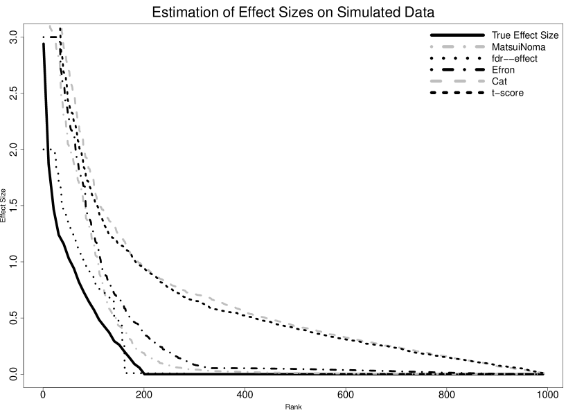
Figure 1: Comparison of effect sizes on simulated data following the Smyth, (2004) model

A comparison of effect size estimation methods using simulated data is shown in Fig. 1. Specifically I compare the effect size estimation using “naives” approaches (simple cat and $t$ –scores) and the more sophisticated ones described in the previous section abbreviated as MatsuiNoma, Efron and fdr–effect respectively. For the methods MatsuiNoma and Efron I use the implementations offered by the authors, for fdr–effect I perform cat–score and fdr estimation using the R-packages st and fdrtool (Strimmer, 2008a, ). In the real data analysis displayed in Fig. 2 the package locfdr (Efron,, 2004, 2007, 2008) is applied since this allows a straightforward use of an empirical null as it has been suggested in Matsui and Noma, (2011) and Efron, (2004) for this data set.

I follow closely the setup used in Smyth, (2004), Opgen-Rhein and Strimmer, (2007) and Zuber and Strimmer, (2009) to simulate gene expression data. The parameters are chosen in such a way that effect sizes between 1 and 3 are obtained which roughly corresponds to the range considered in the simulation studies of Matsui and Noma, (2011).

The number of statistics was fixed at $d=1000$ with 200 statistics designated to be differentially expressed. The variances across genes were drawn from a scale–inverse–chi– square distribution $\text{Scale-inv-}\chi^{2}(d_{0},s_{0}^{2})$ with $s^{2}_{0}=1$ and $d_{0}=1$, i.e. the variances vary moderately from gene to gene. Furthermore, the difference of means for the differentially expressed genes (1–200) were drawn from a normal distribution with mean zero and the gene-specific variance multiplied with a scale factor set to $0.3$. For the non–differentially expressed genes (201–1000) the difference was set to zero. The data were generated by drawing from group-specific multivariate normal distributions with the given variances and means, employing a block diagonal correlation structure intended to mimic gene expression data. This structure was generated as in Guo et al., (2007) with block size 100 and block entries equal to $0.9^{\left\lvert i-j\right\rvert}$. Furthermore, the sample sizes $n_{1}$ and $n_{2}$ are equal with $n_{1}=n_{2}=8$.

The effect size estimates are plotted in Fig. 1 according to their rank. It is important to note that this does not tell us whether the respective ranking is correct. Thus, even though the effect size estimates of the cat–score and an ordinary $t$–score are very similar, this does not mean that their induced ranking is comparable.

It can be seen that fdr–effect and MastsuiNoma yield good results, while Efron’s method has a higher bias for effect sizes up to 1, a phenomenon already observed by Matsui and Noma, (2011). The “naive” approach using cat–scores is far off for effect sizes up to 1.5. However all methods overestimate large effect sizes. It follows that variable selection methods relying on effect size estimates will generally have a tendency of choosing only a relatively small number of variables in data sets with large effects.

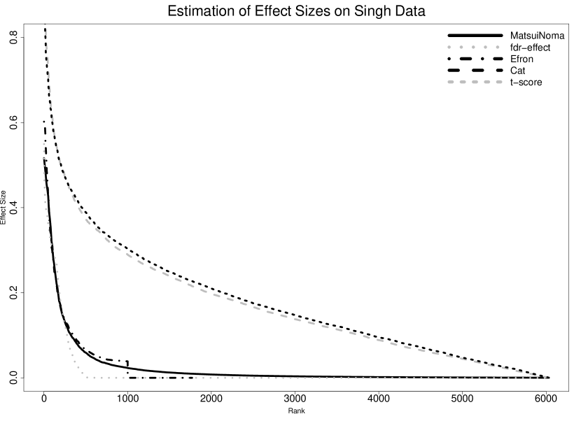
Figure 2: Comparison of effect sizes for the Singh et al., (2002) data

This is in fact a phenomenon already observed by Ahdesmäki and Strimmer, (2010) for the Efron algorithm applied to the Singh et al., (2002) prostate cancer gene expression data. This data consists of gene expression measurements of $d=6033$ genes for $n=102$ patients, of which 52 are cancer patients and 50 are healthy. It has already been analyzed in Efron, (2009) and Matsui and Noma, (2011). Fig. 2 shows the analysis results. As in the simulated data the “naive” approaches are far off, while Efron and MatsuiNoma are quite similar. Note however, that MatsuiNoma gives significantly lower estimates of large effect sizes than Efron a phenomenon already noted in Matsui and Noma, (2011). The fdr–effect method yields similar results to MatsuiNoma for large effect sizes but arrives at zero estimates much faster than MatsuiNoma and Efron. In conclusion all empirical Bayes methods considered seem to give sound results here, while the empirical methods are probably grossly overestimating the effect sizes.

4 Variable Selection and Estimation of the Prediction Rule

4.1 Estimation of the prediction rule and local false discovery rates

For the estimation of the prediction rule (Eq. 2) I mostly employ James-Stein-type estimators as in shrinkage discriminant analysis – SDA, Ahdesmäki and Strimmer, (2010). The group centroids $\boldsymbol{\mu}_{k}$ are estimated by the empirical means, for the correlations $\boldsymbol{P}$ the ridge-type estimator from Schäfer and Strimmer, (2005) is used and the variances $\boldsymbol{V}$ are estimated by the shrinkage estimator from Opgen-Rhein and Strimmer, (2007). Finally the proportions $\pi_{k}$ are obtained by using the frequency estimator from Hausser and Strimmer, (2009). For SDA I employ the implementation provided by the R package sda. The local false discovery rates used in the fdr–effect approach are learned by using the Grenander density estimator and truncated maximum likelihood for the empirical null as in Strimmer, 2008b . As in chapter 3 the implementation offered by the R package fdrtool is employed.

4.2 Variable ranking and selection

4.2.1 Variable ranking

Before being able to select variables a variable ranking needs to be established (obj. (i)). In the two class case this is straightforward since the feature weight vector for class one $\boldsymbol{\omega}_{1}$ corresponds to the effect size vector $\boldsymbol{\omega}^{(1,2)}$ and the feature weight vector for class two $\boldsymbol{\omega}_{2}$ to the effect size vector $-\boldsymbol{\omega}^{(1,2)}$. Thus variables can be ranked according to the absolute value of $\boldsymbol{\omega}^{(1,2)}$. In the the case of multiple classes the situation is more complicated. The feature weight vectors of the different classes need to be summarized in a certain way to obtain the importance of each feature $i$ in class prediction. Here I use the summary statistic $S_{i}$ proposed by (Ahdesmäki and Strimmer,, 2010) and given by

$$S_{i}=\sum_{k=1}^{K}\left(\omega_{\text{cat},i}^{(k,\text{pool})}\right)^{2}\;,$$ (17)

where $\omega_{\text{cat},i}^{(k,\text{pool})}=(1/n_{k}-1/n)^{-1/2}\omega_{i}^{(k,\text{pool})}$. Since false discovery rates are generally assumed to be monotone, Eq. 15 shows that using fdr–effect effect size estimates $\boldsymbol{\omega}^{(k,\text{pool})}_{\text{fdr}}$ would produce the same ranking as the cat–scores if they were used instead of $\boldsymbol{\omega}^{(k,\text{pool})}_{\text{cat}}$ to compute $S_{i}$ in Eq. 17.

4.2.2 Misclassification rate based variable selection

Having obtained estimates $\widehat{\boldsymbol{\omega}}^{(k,l)}_{\text{fdr}}$ of $\boldsymbol{\omega}^{(k,l)}_{\text{fdr}}$ and $\widehat{\pi}_{k}$ of $\pi_{k}$ we can now compute an estimate of the missclassification rate using Eq. 6. Let $\widehat{\boldsymbol{\omega}}^{(k,l)}_{\text{fdr}}(t)$ be the vector of the $t$ top-ranked variables according to the ranking induced by the vector $\boldsymbol{S}$ of all statistics $S_{i}$ given by Eq. 17. We then have an estimate of the misclassification rate which depends on $t$:

$$\widehat{\text{P}}(\text{error})(t)=\sum_{k=1}^{K}\widehat{\text{P}}(\neq k|k)(t)\times\widehat{\text{P}}(k)$$

$$=\sum_{k=1}^{K}\Phi\biggl{(}-\min_{l\neq k}\frac{[\widehat{\boldsymbol{\omega}}^{(k,l)}_{\text{fdr}}(t)]^{T}[\widehat{\boldsymbol{\omega}}^{(k,l)}_{\text{fdr}}(t)]+2\log\biggl{(}\frac{\pi_{k}}{\pi_{l}}\biggr{)}}{2\sqrt{[\widehat{\boldsymbol{\omega}}^{(k,l)}_{\text{fdr}}(t)]^{T}[\widehat{\boldsymbol{\omega}}^{(k,l)}_{\text{fdr}}(t)]}}\biggr{)}\times\widehat{\pi}_{k}\,.$$ (18)

Efron, (2009) performs feature selection by choosing a level $\alpha=0.05$ as a target missclassification rate for the estimate in Eq. 18. Although one could view $\alpha$ as a tuning parameter I follow his suggestion in this regard since experiments with lower results only lead to very large feature sets showing only to a negligible improvement of the classification performance.

After the target error $\alpha$ has been set a feature threshold $t^{*}$ is obtained by including as many features as necessary to reach it, i.e. $\widehat{\text{P}}(\text{error})(t^{*})=\alpha$. Since usually a lot of features are shrunken to zero, it is possible that the target error can not be reached. Then all the features will be included. This however is extremely unlikely to happen in real high dimensional data analysis. Finally all features fulfilling $S_{i}\geq S_{t}^{*}$ are included in the classifier.

5 Analysis of Real and Simulated Data

5.1 Simulations

In this section I compare variable selection based on the misclassification rate (MR) with several other state of the art thresholding variable selection approaches, namely false-non discovery rate (FNDR) thresholding (Ahdesmäki and Strimmer,, 2010), Higher Criticism (HC) thresholding (Donoho and Jin,, 2008) and the PAM algorithm (Tibshirani et al.,, 2003). As a base line classifier I also include the results of classification with all features, i.e. performing no variable selection.

The simulations follow closely the setup of Witten and Tibshirani, (2011). A training set of size 100 and a test set of 1000 samples are created with a dimension of $d=500$ variables. In total 25 runs of each simulation setup are performed.

5.1.1 Simulation setup 1

In this setup there are four classes with equal probability (0.25) no correlation and unit variance. 25 features are differentially expressed in each class with an effect size of 0.7, yielding a total number of 100 differentially expressed features. Since there is no correlation we perform Diagonal Discriminant Analysis (DDA), i.e. LDA with identity covariance $\boldsymbol{\Sigma}=I_{d}$. The results are displayed in Tab. 1.

Table 1: Prediction errors and number of selected features for simulation setup 1, the number in the round brackets is the estimated standard error over 25 runs. the true number of differentially expressed features is 100.

Method	Prediction Error	Features
DDA-MR	0.1077 (0.0177)	156.48 (064.70)
DDA-FNDR	0.2482 (0.1272)	039.24 (023.72)
DDA-HC	0.1880 (0.0626)	152.32 (193.48)
PAM	0.0923 (0.0163)	253.60 (116.26)
DDA-ALL	0.1555 (0.0180)	500.0 (000.00)

It can be seen that thresholding the summary statistic $S$ (Eq. 17) by false-non discovery rates or Higher Criticism yields hardly any significant features in most runs. Consequently the estimated prediction errors are quite high.

Misclassification rate based feature selection as well as PAM however identify features useful for classification. This indicates that ”analytical“ thresholding methods, which do not rely on the optimization of a tuning parameter may not work reliably when the effect sizes are small.

5.1.2 Simulation setup 2

In this simulation I use a Guo et al., (2007) type block correlation with 5 blocks of size $100\times 100$. As in section 3 each block entry is given by $0.9^{\left\lvert i-j\right\rvert}$, thus we have some highly correlated variables within blocks but variables in different blocks are independent.

Note that Witten and Tibshirani, (2011) report to use an entry size of 0.6. This is probably a misprint since my results obtained for PAM are quite similar to the ones reported in their article, while for 0.6 the error of PAM only about 5 %.

There are two classes with equal probability (0.5) and 200 features are differentially expressed with effect size 0.6, all of them are attributed to class 2. Since there is correlation in this setting I perform LDA.

Table 2: Prediction errors and number of selected features for simulation setup 2, the number in the round brackets is the estimated standard error over 25 runs. The true number of differentially expressed features is 200.

Method	Prediction Error	Features
LDA-MR	0.000 (0.000)	63.16 (7.215)
LDA-FNDR	0.000 (0.000)	60.96 (6.567)
LDA-HC	0.000 (0.000)	85.04 (8.677)
PAM	0.088 (0.018)	294.0 (69.43)
LDA-ALL	0.093 (0.014)	500.0 (00.00)

It can be seen in Tab. 2 that all feature selection methods except for PAM, which does not take correlation into account, perform quite well here.

5.2 Gene expression data

In Ahdesmäki and Strimmer, (2010) the relative effectiveness of the FNDR and HC thresholds to select relevant genes in shrinkage discriminant analysis applied to gene expression data has already been compared. I followed their setup here and analyzed four clinical gene expression data sets related to prostate cancer (Singh et al.,, 2002), B-cell lymphoma (Alizadeh et al.,, 2000), colon cancer (Alon et al.,, 1999), and brain cancer (Pomeroy et al.,, 2002).

Specifically, balanced 10-fold cross-validation with 20 repetitions was performed to obtain error estimates and their standard deviations. The number of selected features is inferred by single run of the respective variable selection method on the whole data set. Only for PAM this was repeated several times, since the number of selected variables selected by this algorithm varies considerably between several runs in a row on the same data set.

In Tab. 3 it can bee seen that my approach has a performance similar to the other approaches. Interestingly, the MR approach shows a more “adaptive” feature selection, leading to appropriate feature sets for each problem. In the brain data set a very compact set of features is selected yielding a prediction error which is nonetheless in the range of the other approaches. The same is true for the Lymphoma and Colon data sets. This demonstrates that a variable selection method based on effect sizes leads to compact and yet effective molecular signatures.

Table 3: Analysis of four cancer gene expression data sets with shrinkage discriminant analysis. The number of selected features are determined by a single feature selection run on the whole data set.

Data / Method	Prediction Error	Selected Variables
Prostate ($d=6033,n=102,K=2$)
LDA-MR	0.0630 (0.0050)	134
LDA-FNDR	0.0550 (0.0048)	131
LDA-HC	0.0497 (0.0045)	116
PAM	0.0850 (0.0061)	172-377
Lymphoma ($d=4026,n=62,K=3$)
LDA-MR	0.0211 (0.0039)	34
LDA-FNDR	0.0036 (0.0018)	392
LDA-HC	0.0000 (0.0000)	345
PAM	0.0234 (0.0041)	2796 – 2383
Colon ($d=2000,n=62,K=2$)
LDA-MR	0.1291 (0.0093)	28
LDA-FNDR	0.1278 (0.0088)	168
LDA-HC	0.1233 (0.0087)	122
PAM	0.1160 (0.0921)	13-23
Brain ($d=5597,n=42,K=5$)
LDA-MR	0.1628 (0.0126)	56
LDA-HC	0.1417 (0.0108)	131
LDA-FNDR	0.1525 (0.0120)	102
PAM	0.2023 (0.0118)	42–5587

6 Discussion

In this paper I reviewed and extended statistical techniques related to effect size estimation in linear classification and showed how to use them for variable selection. The fdr–effect method proposed for effect size estimation has been shown to work as well as competing approaches while being conceptually simple and computationally inexpensive. It therefore successfully unites the strengths of the approaches presented in Efron, (2009) and Matsui and Noma, (2011).

Additionally, I gave a unified treatment of the effect size estimation approaches presented in these two papers elucidating similarities not apparent when considering the original publications only.

Variable selection by minimizing the misclassification rate has been somewhat neglected in the literature but I showed in accordance with Dabney and Storey, (2007), Efron, (2009) and Matsui and Noma, (2011) that it is indeed very well suited for real world problems. In addition, it is also much more intuitive than selecting a non-interpretable regularization parameter as for example in the PAM algorithm and leads to compact and interpretable feature sets.

In this work I proposed a conceptually simple and competitive variable selection algorithm that gives priority to genes with large effect sizes and is thus easy to interpret. This has been achieved by extending and combining the ideas of Dabney and Storey, (2007), Efron, (2009) and Matsui and Noma, (2011).

High expectations are associated with the promise of a personalized medicine promising tailored treatments based on genetic and other information of the patient. In order to develop molecular diagnostics guiding these treatments, statistical approaches for effective and interpretable classification are indispensable.

The methodology presented in this article provides interpretability and applicability for biological study and medical use. Reliable effect size estimates allow one to identify genes having discriminative power while variable selection based on these effect size estimates allows the selection of the most important genes for the construction of classification algorithms.

References

- Ahdesmäki and Strimmer, (2010) Ahdesmäki, M. and Strimmer, K. (2010). Feature selection in omics prediction problems using cat scores and false non-discovery rate control. Ann. Appl. Statist., 4:503–519.
- Alizadeh et al., (2000) Alizadeh, A. A., Eisen, M. B., Davis, R. E., Ma, C., Lossos, I. S., Rosenwald, A., Boldrick, J. C., Sabet, H., Tran, T., Yu, X., Powell, J. I., Yang, L., Marti, G. E., Moore, T., Hudson, J., Lu, L., Lewis, D. B., Tibshirani, R., Sherlock, G., Chan, W. C., Greiner, T. C., Weisenburger, D. D., Armitage, J. O., Warnke, R., Levy, R., Wilson, W., Grever, M. R., Byrd, J. C., Botstein, D., Brown, P. O., and Staudt, L. M. (2000). Distinct types of diffuse large B-cell lymphoma identified by gene expression profiling. Nature, 403:503–511.
- Alon et al., (1999) Alon, U., Barkai, N., Notterman, D. A., Gish, K., Ybarra, S., Mack, D., and Levine, A. (1999). Broad patterns of gene expression revealed by clustering analysis of tumor and normal colon tissues probed by oligonucleotide arrays. Proc. Natl. Acad. Sci. USA, 96:6745–6750.
- Cao et al., (2011) Cao, K.-A. L., Boitart, S., and Besse, P. (2011). Sparse pls discriminant analysis: biologically relevant feature selection and graphical displays for multiclass problems. BMC Bioinformatics, 12:253.
- Dabney and Storey, (2007) Dabney, A. R. and Storey, J. D. (2007). Optimality driven nearest centroid classification from genomic data. PLoS ONE, 2:e1002.
- Dawid, (1994) Dawid, A. P. (1994). Selection paradoxes of bayesian inference. Multivariate analysis and its applications (Hong Kong, 1992), volume 24 of IMS Lecture Notes Monogr. Ser. Hayward, CA: Inst. Math. Statist., pages 211–220.
- Donoho and Jin, (2008) Donoho, D. and Jin, J. (2008). Higher criticism thresholding: optimal feature selection when useful features are rare and weak. Proc. Natl. Acad. Sci. USA, 105:14790–15795.
- Efron, (2004) Efron, B. (2004). Large-scale simultaneous hypothesis testing: the choice of a null hypothesis. J. Amer. Statist. Assoc., 99:96–104.
- Efron, (2007) Efron, B. (2007). Size, power and false discovery rates. Ann. Applied Statistics, 35:1351–1377.
- Efron, (2008) Efron, B. (2008). Microarrays, empirical Bayes, and the two-groups model. Statist. Sci., 23:1–22.
- Efron, (2009) Efron, B. (2009). Empirical Bayes estimates for large-scale prediction problems. J. Amer. Statist. Assoc., 104:1015–1028.
- Guo et al., (2007) Guo, Y., Hastie, T., and Tibshirani, T. (2007). Regularized discriminant analysis and its application in microarrays. Biostatistics, 8:86–100.
- Hand, (2006) Hand, D. J. (2006). Classifier technology and the illusion of progress. Statist. Sci., 21:1–14.
- Hausser and Strimmer, (2009) Hausser, J. and Strimmer, K. (2009). Entropy inference and the James-Stein estimator, with application to nonlinear gene association networks. J. Mach. Learn. Res., 10:1469–1484.
- Kim and Simon, (2011) Kim, I. K. and Simon, R. (2011). Probabilistic classifiers with high-dimensional data. Biostatistics, 12:399 – 412.
- Klaus and Strimmer, (2012) Klaus, B. and Strimmer, K. (2012). Signal identification for rare and weak features: higher criticism or false discovery rates? Biostatistics, in press.
- Matsui and Noma, (2011) Matsui, S. and Noma, H. (2011). Estimation and selection in high-dimensional genomic studies for developing molecular diagnostics. Biostatistics, 12:223– – 233.
- Opgen-Rhein and Strimmer, (2007) Opgen-Rhein, R. and Strimmer, K. (2007). Accurate ranking of differentially expressed genes by a distribution-free shrinkage approach. Statist. Appl. Genet. Mol. Biol., 6:9.
- Pang et al., (2009) Pang, H., Tong, T., and Zhao, H. (2009). Shrinkage-based diagonal discriminant analysis and its applications in high-dimensional data. Biometrics, 65:1021–1029.
- Pomeroy et al., (2002) Pomeroy, S. L., Tamayo, P., Gaasenbeek, M., Sturla, L. M., Angelo, M., McLaughlin, M. E., Kim, J. Y. H., Goumnerova, L. C., Black, P. M., Lau, C., Allen, J. C., Zagzag, D., Olson, J. M., Curran, T., Wetmore, C., Biegel, J. A., Poggio, T., Mukherjee, S., Rifkin, R., Califano, A., Stolovitzky, G., Louis, D. N., Mesirov, J. P., Lander, E. S., and Golub, T. R. (2002). Prediction of central nervous system embryonal tumour outcome based on gene expression. Nature, 415:436–442.
- Schäfer and Strimmer, (2005) Schäfer, J. and Strimmer, K. (2005). A shrinkage approach to large-scale covariance matrix estimation and implications for functional genomics. Statist. Appl. Genet. Mol. Biol., 4:32.
- Schwender et al., (2008) Schwender, H., Ickstadt, K., and Rahnenführer, J. (2008). Classification with high-dimensional genetic data: assigning patients and genetic features to known classes. Biometr. J., 50:911–926.
- Senn, (2008) Senn, S. (2008). A note concerning a selection “paradox” of Dawid’s. The American Statistician, 62:206–210.
- Shao et al., (2011) Shao, J., Wang, Y., Deng, X., and Wang, S. (2011). Sparse linear discriminant analysis by thresholdig for high dimensional data. Annals of Statistics, 39:1241–1265.
- Singh et al., (2002) Singh, D., Febbo, P. G., Ross, K., Jackson, D. G., Manola, J., Ladd, C., Tamayo, P., Renshaw, A. A., D’Amico, A. V., Richie, J. P., Lander, E. S., Loda, M., Kantoff, P. W., Golub, T. R., and Sellers, W. R. (2002). Gene expression correlates of clinical prostate cancer behavior. Cancer Cell, 1:203–209.
- Slawski et al., (2008) Slawski, M., Daumer, M., and Boulesteix, A.-L. (2008). CMA - a comprehensive Bioconductor package for supervised classification with high dimensional data. BMC Bionformatics, 9:439.
- Smyth, (2004) Smyth, G. K. (2004). Linear models and empirical Bayes methods for assessing differential expression in microarray experiments. Statist. Appl. Genet. Mol. Biol., 3:3.
- (28) Strimmer, K. (2008a). fdrtool: a versatile R package for estimating local and tail area-based false discovery rates. Bioinformatics, 24:1461–1462.
- (29) Strimmer, K. (2008b). A unified approach to false discovery rate estimation. BMC Bioinformatics, 9:303.
- Tibshirani et al., (2003) Tibshirani, R., Hastie, T., Narsimhan, B., and Chu, G. (2003). Class prediction by nearest shrunken centroids, with applications to DNA microarrays. Statist. Sci., 18:104–117.
- Witten and Tibshirani, (2011) Witten, D. M. and Tibshirani, R. (2011). Penalized classification using Fisher’s linear discriminant. J. R. Statist. Soc. B, 73:753–772.
- Xiaosheng and Simon, (2011) Xiaosheng, W. and Simon, R. (2011). Microarray-based cancer prediction using single genes. BMC Bioinformatics, 12:391.
- Zuber and Strimmer, (2009) Zuber, V. and Strimmer, K. (2009). Gene ranking and biomarker discovery under correlation. Bioinformatics, 25:2700–2707.