Mott Insulator-Superfluid Transition in a Generalized Bose-Hubbard Model with Topologically Non-trivial Flat-Band

Abstract

In this paper, we studied a generalized Bose-Hubbard model on a checkerboard lattice with topologically nontrivial flat-band. We used mean-field method to decouple the model Hamiltonian and obtained phase diagram by Landau theory of second-order phase transition. We further calculate the energy gap and the dispersion of quasi-particle or quasi-hole in Mott insulator state and found that in strong interaction limit the quasi-particles or the quasi-holes also have flat bands.

I INTRODUCTION

The Mott insulator (MI) – superfluid transition (SF) of ultracold bosons in optical latticesJaksch ; Greiner has become a hot topic in quantum simulationBuluta and a great deal of works have been done. The Bose-Hubbard model proposed in Ref. Fisher have been widely investigated both theoretically and experimentally so that a comprehensive understanding of this many-body system can be achieved.

On the other hand, the states with topological order become another hot topic and have been explored from different aspects. Since first discovered in two-dimensional electron gas with Landau levels in strong magnetic field, integer and fractional quantum Hall effect (IQHE and FQHE) have attracted great attention. Haldane pointed out that IQHE may appear in honeycomb lattice without Landau levelshaldane . However, FQHE in a lattice model without Landau levels had not been discovered until the proposal of the lattice models with topologically nontrivial flat-band based on the mechanism of quadratic band touchingTang ; Sun ; Neupert . In these lattice models (kagóme lattice, $\pi$-flux square lattice and honeycomb lattice), the hoppings of next-nearest or next-next-nearest (NNN and NNNN) neighbor besides nearest neighbor(NN) are introduced to achieve the flat-bands with a high flatness ratio (the flatness ratio defined as the band gap over the band width) in different lattice models. To obtain FQHE states, people always consider these tight-binding models with the NN and NNN repulsions for fermions and corresponding tight-binding models under a hard-core condition for bosons. Then the numerical results confirm the existence of topologically nontrivial flat-band. For example, in Ref.(Wang ), in an extended bosonic Haldane model with the NN and NNN repulsions under a hard-core condition, the $\nu=1/2$ and the $\nu=1/4$ bosonic FQHE states are predicted.

So we may ask questions : in a bosonic lattice model of topologically nontrivial flat-band with on-site Coulomb interaction, what’s the ground state and whether the topologically nontrivial flat-band affects the superfluid state and Mott state? This becomes the starting point of this paper. In this paper, we study the MI-SF transition in a bosonic system of the checkerboard model with topological flat-bandSun , of which there is no NN or NNN repulsions. Instead, we replace the hard-core condition by a tunable on-site repulsive interaction and consider a generalized Bose-Hubbard model with the hopping parameters as that of the models with topologically nontrivial flat-band. We will use the mean field approach to obtain the quantum phase transitions between MI phase and SF phaseOosten ; Lim . Then the elementary excitations are studied in Mott insulator state. We derive the energy gap and the dispersion of quasi-particle or quasi-hole.

The paper is organized as follow: We first introduce the generalized Bose-Hubbard model with the hopping parameters as that of the models with topologically nontrivial flat-band in Sec. II, then study this model in Sec. III by mean field approach. And in Sec. III we obtain the phase diagrams of this model. The properties of collective modes are analyzed in the last subsection in Sec. IV. Finally we draw the conclusion in Sec. V.

II The model Hamiltonian

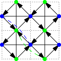
Figure 1: The scheme of the square lattice, of which the two different lattice sites in blue or green colors are two sublattices A and B. The NN hoppings $t$ are represented by lines with arrows whose directions are sign of the phase $\varphi$. The dotted lines represent the NNN hoppings which are $-t^{\prime}$ between green sites(sublattice A) and $t^{\prime}$ between blue sites(sublattice B). Two dashed lines representing the NNNN hoppings are displayed in the scheme, too.

We first generalize the fermionic topological flat-band model to bosonic system with the Hamiltonian

$$H =-t\sum_{\langle j,l\rangle}\left[b_{\mathbf{r}_{j}}^{\dagger}b_{\mathbf{r}_{l}}\exp\left(i\varphi_{jl}\right)\right]\pm t^{\prime}\sum_{\langle\langle j,l\rangle\rangle}b_{\mathbf{r}_{j}}^{\dagger}b_{\mathbf{r}_{l}}$$

$$-t^{\prime\prime}\sum_{\langle\langle\langle j,l\rangle\rangle\rangle}b_{\mathbf{r}_{j}}^{\dagger}b_{\mathbf{r}_{l}}+\frac{U}{2}\sum_{j}n_{\mathbf{r}_{j}}(n_{\mathbf{r}_{j}}-1)$$ (1)

$$-\mu\sum_{j}b_{\mathbf{r}_{j}}^{\dagger}b_{\mathbf{r}_{j}}+\text{H.c.}$$

where $b_{\mathbf{r}_{j}}^{\dagger}$ ($b_{\mathbf{r}_{j}}$) is the bosonic creation (annihilation) operator of the $j$-th site with position vector $\mathbf{r}_{j}$. $\langle j,l\rangle$, $\langle\langle j,l\rangle\rangle$ and $\langle\langle\langle j,l\rangle\rangle\rangle$ denote that $j$ and $l$ are the NN, NNN and NNN sites, respectively. The phase factor of NN hopping $\varphi_{jl}$ equals $\pm\varphi$ (Figure 1). $t$, $t^{\prime},$ $t^{\prime\prime}$ are the hopping parameters for NN hoppings, NNN hoppings, NNNN hoppings, respectively. $U$ is the on-site interaction strength and $\mu$ is the chemical potential.

In the following parts we will use mean field approach to calculate above bosonic topological flat-band model. In addition, to show the effect of the flat-band on MI-SF transition, we also calculate the generalized Bose-Hubbard model without topological flat-band and compare their phase diagram.

III Mean-field approximation and phase diagram

In this section we derive the decoupled effective Hamiltonian from Eq.(1) by mean-field approximation and calculate the corresponding perturbation energy up to second order. Then the equation of critical line of MI-SF transition is obtained by Landau theory of phase transition.

III.1 Mean-field approximation

In the strong-coupling Limit ($t\ll U$), a localized superfluid order parameter $\psi_{\mathbf{r}_{j}}=\langle b_{\mathbf{r}_{j}}^{\dagger}\rangle=\langle b_{\mathbf{r}_{j}}\rangle$ is introduced so as to rewrite the hopping terms by a consistent mean-field method as

$$b_{\mathbf{r}_{j}}^{\dagger}b_{\mathbf{r}_{l}}\simeq b_{\mathbf{r}_{j}}^{\dagger}\psi_{\mathbf{r}_{l}}+b_{\mathbf{r}_{l}}\psi_{\mathbf{r}_{j}}-\psi_{\mathbf{r}_{j}}\psi_{\mathbf{r}_{l}}.$$ (2)

Thus the Hamiltonian can be written as

$$H^{\text{eff}}\ =-t\cos\varphi\sum_{j}\sum_{l=1}^{z}\left[b_{\mathbf{r}_{j}}^{\dagger}+b_{\mathbf{r}_{j}}-\psi_{\mathbf{r}_{j}}\right]\psi_{\mathbf{r}_{j}+\boldsymbol{\tau}_{l}}$$

$$\pm t^{\prime}\sum_{j}\sum_{l=1}^{z^{\prime}}\left[b_{\mathbf{r}_{j}}^{\dagger}+b_{\mathbf{r}_{j}}-\psi_{\mathbf{r}_{j}}\right]\psi_{\mathbf{r}_{j}+\boldsymbol{\tau}_{l}^{\prime}}$$

$$-t^{\prime\prime}\sum_{j}\sum_{l=1}^{z^{\prime\prime}}\left[b_{\mathbf{r}_{j}}^{\dagger}+b_{\mathbf{r}_{j}}-\psi_{\mathbf{r}_{j}}\right]\psi_{\mathbf{r}_{j}+\boldsymbol{\tau}_{l}^{\prime\prime}}$$

$$+\frac{U}{2}\sum_{j}n_{\mathbf{r}_{j}}(n_{\mathbf{r}_{j}}-1)-\mu\sum_{j}b_{\mathbf{r}_{j}}^{\dagger}b_{\mathbf{r}_{j}}\ ,$$ (3)

where $z,$ $z^{\prime},$ $z^{\prime\prime}$ denote the coordination numbers of NN, NNN and NNNN hoppings and $\boldsymbol{\tau}_{l},$ $\boldsymbol{\tau}_{l}^{\prime},$ $\boldsymbol{\tau}_{l}^{\prime\prime}$ are the corresponding translation vectors, respectively. Hence the decoupled effective Hamiltonian can be rewritten with respect to $\mathbf{r}_{j}$ as

$$H_{\mathbf{r}_{j}}^{\text{eff}} =-zt\cos\varphi(b_{\mathbf{r}_{j}}^{\dagger}+b_{\mathbf{r}_{j}}-\psi_{\mathbf{r}_{j}})\psi_{\mathbf{r}_{j}+\boldsymbol{\tau}}$$

$$-zt^{\prime\prime}(b_{\mathbf{r}_{j}}^{\dagger}+b_{\mathbf{r}_{j}}-\psi_{\mathbf{r}_{j}})\psi_{\mathbf{r}_{j}+\boldsymbol{\tau}^{\prime\prime}}$$

$$+\frac{U}{2}n_{\mathbf{r}_{j}}(n_{\mathbf{r}_{j}}-1)-\mu n_{\mathbf{r}_{j}}\ .$$ (4)

Since there are two sublattices of this lattice (A and B), we can define two order parameters $\psi_{A}=\langle b_{\mathbf{r}_{j\in A}}^{\dagger}\rangle$ and $\psi_{B}=\langle b_{\mathbf{r}_{j\in B}}^{\dagger}\rangle$ that correspond to the Bose condensations on A site and on B site, respectively. The order parameters satisfy the condition $\psi_{A}=\psi_{\mathbf{r}_{j}}=\psi_{\mathbf{r}_{j}+\boldsymbol{\tau}^{\prime}}=\psi_{\mathbf{r}_{j}+\boldsymbol{\tau}^{\prime\prime}}$ and $\psi_{B}=\psi_{\mathbf{r}_{j}+\boldsymbol{\tau}}$ if site $j$ denotes an A site and similar condition for B site can be obtained if we substitute A with B. Then we can construct an effective Hamiltonian of a two-site cell with the condition $z=z^{\prime}=z^{\prime\prime}$ as

$$H^{\text{eff}} =(zt)^{-1}(H_{1}+H_{2})=(zt)^{-1}(H^{\text{eff}}_{\mathbf{r}_{j}}+H^{\text{eff}}_{\mathbf{r}_{j}+\boldsymbol{\tau}})$$

$$=\frac{\overline{U}}{2}\left(n_{1}^{2}+n_{2}^{2}-n\right)-\bar{\mu}n+2\psi_{1}\psi_{2}\cos\varphi$$

$$+\bar{t}^{\prime\prime}\psi_{1}^{2}+\bar{t}^{\prime\prime}\psi_{2}^{2}+(\psi_{2}\cos\varphi+\bar{t}^{\prime\prime}\psi_{1})V_{1}$$

$$+(\psi_{1}\cos\varphi+\bar{t}^{\prime\prime}\psi_{2})V_{2}\ ,$$ (5)

where $\psi_{1}=\psi_{A}$, $\psi_{2}=\psi_{B}$ and $\overline{U}=\frac{U}{zt}$, $\bar{\mu}=\frac{\mu}{zt}$, $\bar{t}^{\prime\prime}=\frac{t^{\prime\prime}}{zt}$, $V_{i}=-(b_{i}^{\dagger}+b_{i})$. We then divide the effective Hamiltonian into two terms: the unperturbed term

$$H^{(0)}=\frac{\overline{U}}{2}(n_{1}^{2}+n_{2}^{2}-n)-\bar{\mu}n+2\psi_{1}\psi_{2}\cos\varphi+\bar{t}^{\prime\prime}\psi_{1}^{2}+\bar{t}^{\prime\prime}\psi_{2}^{2}\ ,$$ (6)

and the perturbation term

$$H^{\prime}=(\psi_{1}\bar{t}^{\prime\prime}+\psi_{2}\cos\varphi)V_{1}+(\psi_{1}\cos\varphi+\psi_{2}\bar{t}^{\prime\prime})V_{2}\ .$$ (7)

Hence the unperturbed ground energy is given by

$$E^{(0)}=\frac{\overline{U}}{2}(n_{1}^{2}+n_{2}^{2}-n)-\bar{\mu}n+2\psi_{1}\psi_{2}\cos\varphi+\bar{t}^{\prime\prime}\psi_{1}^{2}+\bar{t}^{\prime\prime}\psi_{2}^{2}\ .$$ (8)

As first-order perturbation of energy vanishes, we get second-order energy perturbation

$$E^{(2)} =-\frac{(\psi_{2}\cos\varphi+\bar{t}^{\prime\prime}\psi_{1})^{2}(\overline{U}+\bar{\mu})}{(-n_{1}\overline{U}+\bar{\mu})\left[(n_{1}-1)\overline{U}-\bar{\mu}\right]}$$

$$-\frac{(\psi_{1}\cos\varphi+\bar{t}^{\prime\prime}\psi_{2})^{2}(\overline{U}+\bar{\mu})}{(-n_{2}\overline{U}+\bar{\mu})\left[(n_{2}-1)\overline{U}-\bar{\mu}\right]}\ .$$ (9)

Thus energy up to second-order is obtained as

$$E(\psi_{1},\psi_{2})\approx a_{0}+a_{2}\psi_{1}^{2}+c_{2}\psi_{1}\psi_{2}+b_{2}\psi_{2}^{2}+\mathcal{O}(\psi^{2})\ ,$$ (10)

where

$$a_{0}= \frac{\overline{U}}{2}(n_{1}^{2}+n_{2}^{2}-n)-\bar{\mu}n$$

$$a_{2}= \bar{t}^{\prime\prime}-\frac{\bar{t}^{\prime\prime 2}(\overline{U}+\bar{\mu})}{(-n_{1}\overline{U}+\bar{\mu})\left[(n_{1}-1)\overline{U}-\bar{\mu}\right]}$$

$$-\frac{(\overline{U}+\bar{\mu})\cos^{2}\varphi}{(-n_{2}\overline{U}+\bar{\mu})\left[(n_{2}-1)\overline{U}-\bar{\mu}\right]}$$

$$b_{2}= \bar{t}^{\prime\prime}-\frac{(\overline{U}+\bar{\mu})\cos^{2}\varphi}{(-n_{1}\overline{U}+\bar{\mu})\left[(n_{1}-1)\overline{U}-\bar{\mu}\right]}$$

$$-\frac{\bar{t}^{\prime\prime 2}(\overline{U}+\bar{\mu})}{(-n_{2}\overline{U}+\bar{\mu})\left[(n_{2}-1)\overline{U}-\bar{\mu}\right]}$$

$$c_{2}= 2\cos\varphi-\frac{2\bar{t}^{\prime\prime}(\overline{U}+\bar{\mu})\cos\varphi}{(-n_{1}\overline{U}+\bar{\mu})\left[(n_{1}-1)\overline{U}-\bar{\mu}\right]}$$

$$-\frac{2\bar{t}^{\prime\prime}(\overline{U}+\bar{\mu})\cos\varphi}{(-n_{2}\overline{U}+\bar{\mu})\left[(n_{2}-1)\overline{U}-\bar{\mu}\right]}\ .$$ (11)

III.2 Phase diagram

The MI-SF phase transition occurs on the condition when Gaussian curvature is zero at the point $\psi_{1}=0,\psi_{2}=0$, namely

$$\frac{\partial^{2}E}{\partial\psi_{1}^{2}}\bigg{|}_{(0,0)}\frac{\partial^{2}E}{\partial\psi_{2}^{2}}\bigg{|}_{(0,0)}-\left(\frac{\partial^{2}E}{\partial\psi_{1}\partial\psi_{2}}\bigg{|}_{(0,0)}\right)^{2}=0\ .$$ (12)

It implies that

$$4a_{2}b_{2}-c_{2}^{2}=0\ .$$ (13)

With $n_{1}=n_{2}=n$, considering the symmetry between two sublattices, $a_{2}=b_{2}$, we have $2a_{2}=\pm c_{2}$. Solve the equation for $\bar{\mu}$, we can get the boundary condition

$$\bar{\mu}= \frac{1}{2}\Bigg{[}(2n-1)\overline{U}-(\bar{t}^{\prime\prime}-\cos\varphi)$$

$$\pm\sqrt{\overline{U}^{2}-2(2n+1)(\bar{t}^{\prime\prime}-\cos\varphi)\overline{U}+(\bar{t}^{\prime\prime}-\cos\varphi)^{2}}\Bigg{]}\ .$$ (14)

for negative $\overline{U}$, namely positive $U$ as $t=-1$.

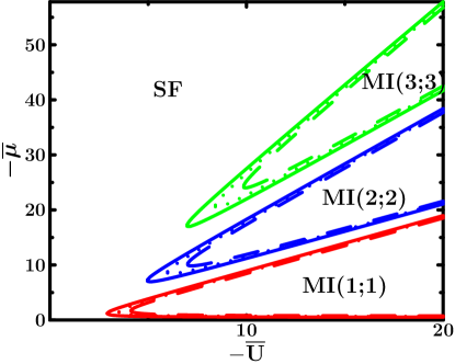
Figure 2: The phase diagram of MI-SF transition. The solid lines are the phase boundaries of topological non-trivial flat-band case with $t=-1$, $\bar{t}^{\prime}=-\frac{1}{2+\sqrt{2}}$, $\bar{t}^{\prime\prime}=\frac{1}{2+2\sqrt{2}}$ and $\varphi=\frac{\pi}{4}$. The dashed lines are the phase boundaries of the case with $t=-1$, $\bar{t}^{\prime}=0$, $\bar{t}^{\prime\prime}=0$ and $\varphi=\frac{\pi}{4}$. The dotted lines are phase boundaries of the case with $t=-1$, $\bar{t}^{\prime}=-\frac{1}{2(2+\sqrt{2})}$, $\bar{t}^{\prime\prime}=\frac{1}{2(2+2\sqrt{2})}$ and $\varphi=\frac{\pi}{4}$. On the other hand, the red lines represent phase boundaries of configuration $\{1;1\}$, blue ones $\{2;2\}$, and green ones $\{3;3\}$.

The phase diagram is displayed in Figure 2. In Figure 2, there are three MI-SF phase transition lines for each particle number configuration. The particle number configuration $\{n_{1};n_{2}\}$ represents that there are $n_{1}$ bosons on each A lattice site while $n_{2}$ bosons on each B lattice site. Due to the existence of inversion symmetry, we have $n_{1}=n_{2}$.

The solid lines are phase boundaries of the flat-band case with $t=-1$, $\bar{t}^{\prime}=-\frac{1}{2+\sqrt{2}}$, $\bar{t}^{\prime\prime}=\frac{1}{2+2\sqrt{2}}$ and $\varphi=\frac{\pi}{4}$. We can see that quantum phase transition occurs when $\overline{U}$ increases by fixing $\bar{\mu}$. The phase diagram is similar to the traditional Bose-Hubbard model with only nearest hopping termOosten ; Lim . To show the effect of flat-band, we also calculate other two cases without topological flat-bands: the $\varphi$-flux Bose-Hubbard model with only nearest hopping term or $\bar{t}^{\prime}={t}^{\prime\prime}=0,$ $\varphi=\frac{\pi}{4}$ (the dashed lines) and the generalized Bose-Hubbard model with smaller NNN and NNNN hopping parameters compared with flat-band case, namely $\varphi=\frac{\pi}{4}$ and $\bar{t}^{\prime}=-\frac{1}{2(2+\sqrt{2})}$, $\bar{t}^{\prime\prime}=\frac{1}{(2+2\sqrt{2})}$ (the dotted lines). From these results, we can see that, the superfluid phase of flat-band model becomes larger compared with the $\varphi$-flux Bose-Hubbard model with only nearest hopping term.

IV Collective modes in Mott phase

In this section, we first derive the effective action of this bosonic checkerboard model of flat-band. Then we calculate the dispersion and the energy gap of excitations in Mott phase.

IV.1 The effective action

With the complex functions $b_{i}^{\ast}(\tau)$ and $b_{i}(\tau)$ defined, the grand canonical partition function can be written as

$$Z=\text{Tr}{e^{-\beta\hat{H}}}=\int\mathcal{D}b^{\ast}\mathcal{D}be^{-S[b^{\ast},b]/\hbar}\ ,$$ (15)

where $\mathcal{D}b^{\ast}$ and $\mathcal{D}b$ denote functional integration for $b^{\ast}$ and $b$, respectively. The action $S[b^{\ast},b]$ is given by

$$S[b^{\ast},b] =\int_{0}^{\hbar\beta}d\tau\Bigg{[}\sum_{i}b_{i}^{\ast}(\tau)\left(\hbar\frac{\partial}{\partial\tau}-\mu\right)b_{i}(\tau)$$

$$-\sum_{ij}t_{ij}b_{i}^{\ast}(\tau)b_{j}(\tau)$$

$$+\frac{1}{2}U\sum_{i}b_{i}^{\ast}(\tau)b_{i}^{\ast}(\tau)b_{i}(\tau)b_{i}(\tau)\Bigg{]}\ ,$$ (16)

with $\beta=\frac{1}{k_{B}T}$, $k_{B}$ the Boltzmann constant, and $T$ the temperature. With a Hubbard-Stratonovich transformation, we can rewrite the action as

$$S[b^{*},b,\psi^{*},\psi] = S[b^{*},b]+\int_{0}^{\hbar\beta}d\tau\sum_{ij}\big{(}\psi_{i}^{*}(\tau)-b_{i}^{*}(\tau)\big{)}t_{ij}\big{(}\psi_{j}(\tau)-b_{j}(\tau)\big{)}$$ (17)

$$= \int_{0}^{\hbar\beta}d\tau\Bigg{[}\sum_{i}b_{i}^{*}(\tau)\left(\hbar\frac{\partial}{\partial\tau}-\mu\right)b_{i}(\tau)+\frac{1}{2}U\sum_{i}b_{i}^{*}(\tau)b_{i}^{*}(\tau)b_{i}(\tau)b_{i}(\tau)$$

$$-\sum_{ij}\big{(}b_{i}^{*}(\tau)t_{ij}\psi_{j}(\tau)+\psi_{i}^{*}(\tau)t_{ij}b_{j}(\tau)\big{)}+\sum_{ij}\psi_{i}^{*}(\tau)t_{ij}\psi_{j}(\tau)\Bigg{]}\ ,$$

where $\psi^{\ast}$ and $\psi$ are the order parameter fields. Hnece we have

$$e^{-S^{\text{eff}}[\psi^{\ast},\psi]}=\exp{\left\{-\frac{1}{\hbar}\int_{0}^{\hbar\beta}d\tau\sum_{ij}t_{ij}\psi_{i}^{\ast}(\tau)\psi_{j}(\tau)\right\}}$$

$$\times\int\mathcal{D}b^{\ast}\mathcal{D}b\exp\Bigg{\{}-S^{(0)}[b^{\ast},b]/\hbar-\frac{1}{\hbar}\int_{0}^{\hbar\beta}d\tau$$

$$\left(-\sum_{ij}t_{ij}\big{(}b_{i}^{\ast}(\tau)\psi_{j}(\tau)+\psi_{i}^{\ast}(\tau)b_{j}(\tau)\big{)}\right)\Bigg{\}}\ ,$$ (18)

where $S^{(0)}$ is the action with no hoping terms.

Using the cumulate expansion formula

$$\left\langle e^{A_{i}}\right\rangle=e^{\left\langle A_{i}\right\rangle+\frac{1}{2}\left(\left\langle A_{i}^{2}\right\rangle-\left\langle A_{i}\right\rangle^{2}\right)+\ldots}\ ,$$ (19)

we can get the effective action up to second-order

$$S^{\text{eff}}[\psi^{\ast},\psi]\approx S^{(0)}+S^{(2)}\ ,$$ (20)

where perturbation term is

$$S^{(2)}[\psi^{*},\psi] = \int_{0}^{\hbar\beta}d\tau\sum_{ij}t_{ij}\psi_{i}^{*}(\tau)\psi_{j}(\tau)-\frac{1}{2\hbar}\left<\left(\int_{0}^{\hbar\beta}d\tau\sum_{ij}t_{ij}\big{[}b_{i}^{*}(\tau)\psi_{j}(\tau)+\psi_{i}^{*}(\tau)b_{j}(\tau)\big{]}\right)^{2}\right>_{S^{(0)}}$$ (21)

$$= \int_{0}^{\hbar\beta}d\tau\sum_{ij}t_{ij}\psi_{i}^{*}(\tau)\psi_{j}(\tau)$$

$$-\frac{1}{2\hbar}\left<\int_{0}^{\hbar\beta}\int_{0}^{\hbar\beta}d\tau d\tau^{\prime}\sum_{iji^{\prime}j^{\prime}}t_{ij}t_{i^{\prime}j^{\prime}}\big{[}b_{i}^{*}(\tau)\psi_{j}(\tau)+\psi_{i}^{*}(\tau)b_{j}(\tau)\big{]}\big{[}b_{i^{\prime}}^{*}(\tau^{\prime})\psi_{j^{\prime}}(\tau^{\prime})+\psi_{i^{\prime}}^{*}(\tau^{\prime})b_{j^{\prime}}(\tau^{\prime})\big{]}\right>_{S^{(0)}}\ .$$

With the correlations in the unperturbed system

$$\left\langle b_{i}^{\ast}b_{j}^{\ast}\right\rangle_{S^{(0)}}=\left\langle b_{i}b_{j}\right\rangle_{S^{(0)}}=0$$

$$\left\langle b_{i}^{\ast}b_{j}\right\rangle_{S^{(0)}}=\left\langle b_{i}b_{j}^{\ast}\right\rangle_{S^{(0)}}=\left\langle b_{i}b_{i}^{\ast}\right\rangle_{S^{(0)}}\delta_{ij}\ ,$$ (22)

we get

$$S^{(2)}[\psi^{\ast},\psi]=\int_{0}^{\hbar\beta}d\tau\sum_{ij}\psi_{i}^{\ast}t_{ij}\psi_{j}-\frac{1}{\hbar}\int_{0}^{\hbar\beta}\int_{0}^{\hbar\beta}d\tau d\tau^{\prime}$$

$$\sum_{iji^{\prime}j^{\prime}}t_{ij}t_{i^{\prime}j^{\prime}}\psi_{j}^{\ast}(\tau)\left\langle T_{\tau}[b_{i}(\tau)b_{i^{\prime}}^{\ast}(\tau^{\prime})]\right\rangle_{S^{(0)}}\psi_{j^{\prime}}(\tau^{\prime})\ .$$ (23)

In general, the first term of above equation can be written as

$$\sum_{ij}t_{ij}\psi_{i}^{\ast}\psi_{j}=\sum_{\mathbf{k}}\bigg{(}\big{(}\psi_{A\mathbf{k}}^{\ast}(\tau),\psi_{B\mathbf{k}}^{\ast}(\tau)\big{)}\mathcal{H}\Big{(}\begin{tabular}[c]{c}$\psi_{A\mathbf{k}}(\tau)$\\ $\psi_{B\mathbf{k}}(\tau)$\end{tabular}\ \Big{)}\bigg{)}\ ,$$ (24)

by a Fourier transformation, where $T_{\tau}$ is the imaginary-time order operator. And the quadratic term becomes

$$\sum_{jii^{\prime}j^{\prime}}t_{ji}t_{i^{\prime}j^{\prime}}\psi_{\mathbf{r}_{j}}^{\ast}(\tau)\left\langle T_{\tau}[b_{\mathbf{r}_{i}}(\tau)b_{\mathbf{r}_{i^{\prime}}}^{\ast}(\tau^{\prime})]\right\rangle_{S^{(0)}}\psi_{\mathbf{r}_{j^{\prime}}}(\tau^{\prime})$$

$$=\sum_{jij^{\prime}}t_{ji}t_{ij^{\prime}}\psi_{\mathbf{r}_{j}}^{\ast}(\tau)\left\langle T_{\tau}[b_{\mathbf{r}_{i}}(\tau)b_{\mathbf{r}_{i}}^{\ast}(\tau^{\prime})]\right\rangle_{S^{(0)}}\psi_{\mathbf{r}_{j^{\prime}}}(\tau^{\prime})$$

$$=\left\langle T_{\tau}[b_{\mathbf{r}_{i}}(\tau)b_{\mathbf{r}_{i}}^{\ast}(\tau^{\prime})]\right\rangle_{S^{(0)}}\sum_{jij^{\prime}}t_{ji}t_{ij^{\prime}}\psi_{\mathbf{r}_{j}}^{\ast}(\tau)\psi_{\mathbf{r}_{j^{\prime}}}(\tau^{\prime})\,.$$ (25)

It can be show that

$$\sum_{jij^{\prime}}t_{ji}t_{ij^{\prime}}\psi_{\mathbf{r}_{j}}^{\ast}(\tau)\psi_{\mathbf{r}_{j}^{\prime}}(\tau^{\prime})$$

$$=\sum_{\mathbf{k}}(\psi_{A\mathbf{k}}^{\ast}(\tau),\psi_{B\mathbf{k}}^{\ast}(\tau))\mathcal{H}^{2}\left(\begin{tabular}[c]{c}$\psi_{A\mathbf{k}}(\tau^{\prime})$\\ $\psi_{B\mathbf{k}}(\tau^{\prime})$\end{tabular}\ \right)\ .$$ (28)

Hence at the transition point where $S^{(0)}$ vanishes, the effective action can be written as

$$S^{\text{eff}}\ =\int_{0}^{\hbar\beta}\sum_{\mathbf{k}}(\psi_{A\mathbf{k}}^{\ast},\psi_{B\mathbf{k}}^{\ast})\mathcal{H}\left(\begin{tabular}[c]{c}$\psi_{A\mathbf{k}}$\\ $\psi_{B\mathbf{k}}$\end{tabular}\ \right)-\frac{1}{\hbar}\int_{0}^{\hbar\beta}\int_{0}^{\hbar\beta}d\tau d\tau^{\prime}$$ (31)

$$\langle T_{\tau}[b(\tau)b^{\ast}(\tau^{\prime})]\rangle\sum_{\mathbf{k}}(\psi_{A\mathbf{k}}^{\ast}(\tau),\psi_{B\mathbf{k}}^{\ast}(\tau))\mathcal{H}^{2}\left(\begin{tabular}[c]{c}$\psi_{A\mathbf{k}}(\tau^{\prime})$\\ $\psi_{B\mathbf{k}}(\tau^{\prime})$\end{tabular}\ \right)\ .$$ (34)

This is consistent with the results of a two-site model in Ref.Lim .

IV.2 Dispersion of collective modes

After obtaining the effective action of this bosonic checkerboard model of flat-band, we calculate the critical point of MI-SF transition and then the dispersion of collective modes.

For the bosonic checkerboard model of flat-band, the hoping terms are given by

$$t_{ij}=t_{ji}^{\ast}=\left\{\begin{tabular}[c]{cc}$te^{i\varphi}$&\mbox{for NN terms, }\\ $\pm t^{\prime}$&\mbox{for NNN terms, }\\ $t^{\prime\prime}$&\mbox{for NNNN terms, }\\ $0$&\mbox{otherwise.}\end{tabular}\ \ \right..$$ (35)

Then the $\mathcal{H}$ matrix was obtained asSun

$$\mathcal{H}= \left[\begin{tabular}[c]{cc}$\mathcal{A}$&$\mathcal{C}^{\ast}$\\ $\mathcal{C}$&$\mathcal{B}$\end{tabular}\ \right]$$ (38)

$$= 4t^{\prime\prime}\cos k_{x}\cos k_{y}I+4t\cos\varphi(\cos\frac{k_{x}}{2}\cos\frac{k_{y}}{2})\sigma_{x}$$

$$+4t\sin\varphi(\sin\frac{k_{x}}{2}\sin\frac{k_{y}}{2})\sigma_{y}+2t^{\prime}(\cos k_{x}-\cos k_{y})\sigma_{z}\ ,$$ (39)

where $I$ and $\sigma_{x}$, $\sigma_{y}$, $\sigma_{z}$ is the identity and Pauli matrices. Hence

$$\mathcal{A} =2t^{\prime}(\cos k_{x}-\cos k_{y})+4t^{\prime\prime}\cos k_{x}\cos k_{y}\ ,$$ (40)

$$\mathcal{B} =-2t^{\prime}(\cos k_{x}-\cos k_{y})+4t^{\prime\prime}\cos k_{x}\cos k_{y}\ ,$$ (41)

$$\mathcal{C} =4t\cos\varphi\cos\frac{k_{x}}{2}\cos\frac{k_{y}}{2}+4it\sin\varphi\sin\frac{k_{x}}{2}\sin\frac{k_{y}}{2}\ .$$ (42)

The $\left\langle T_{\tau}[b(\tau)b^{\ast}(\tau^{\prime})]\right\rangle_{S^{(0)}}$ is just the negative of Matsubara Green’s function and it can be evaluated as

$$\left\langle T_{\tau}[b(\tau)b^{\ast}(\tau^{\prime})]\right\rangle_{S^{(0)}} =\theta(\tau-\tau^{\prime})(n+1)e^{-(-\mu+nU)(\tau-\tau^{\prime})/\hbar}$$

$$+\theta(\tau^{\prime}-\tau)ne^{(\mu-(n-1)U)(\tau^{\prime}-\tau)/\hbar}\ .$$ (43)

After Fourier transformation to Hubbard-Stratonovich fields in the Matsubara frequencies,

$$\psi_{A\mathbf{k}}(\tau) =\frac{1}{\sqrt{\hbar\beta}}\sum_{m}e^{-i\omega\tau}\psi_{A\mathbf{k,\omega_{m}}}$$

$$\psi_{B\mathbf{k}}(\tau) =\frac{1}{\sqrt{\hbar\beta}}\sum_{m}e^{-i\omega\tau}\psi_{B\mathbf{k,\omega_{m}}}\ ,$$ (44)

the effective action is given by

$$S^{\text{eff}}[\psi^{\ast},\psi]$$

$$=\sum_{\mathbf{k},m}(\psi_{A\mathbf{k},m}^{\ast},\psi_{B\mathbf{k},m}^{\ast})\left(\mathcal{H}-\mathcal{H}^{2}f_{\omega_{m}}\right)(\begin{tabular}[c]{c}$\psi_{B\mathbf{k},\omega_{m}}$\\ $\psi_{B\mathbf{k},\omega_{m}}$\end{tabular}\ \ )$$ (47)

$$=\sum_{\mathbf{k},m}(\psi_{A\mathbf{k},m}^{\ast},\psi_{B\mathbf{k},m}^{\ast})(-\hbar\mathbf{G}^{-1}(\mathbf{k},i\omega_{m}))(\begin{tabular}[c]{c}$\psi_{A\mathbf{k},m}$\\ $\psi_{B\mathbf{k},m}$\end{tabular}\ \ )\ ,$$ (50)

where

$$f_{\omega_{m}}=\frac{n+1}{-i\hbar\omega_{m}-\mu+nU}+\frac{n}{i\hbar\omega_{m}+\mu-(n-1)U}\ ,$$ (51)

and

$$\hbar\mathbf{G}^{-1}(\mathbf{k},i\omega_{m})$$

$$=\left(\begin{tabular}[c]{cc}$(\mathcal{A}^{2}+\mathcal{C}^{\ast}\mathcal{C})f_{\omega_{m}}-\mathcal{A}$ \thinspace&$(\mathcal{A}+\mathcal{B})\mathcal{C}^{\ast}f_{\omega_{m}}-\mathcal{C}^{\ast}$\\ $(\mathcal{A}+\mathcal{B})\mathcal{C}f_{\omega_{m}}-\mathcal{C}$ \thinspace&$(\mathcal{B}^{2}+\mathcal{C}^{\ast}\mathcal{C})f_{\omega_{m}}-\mathcal{B}$\end{tabular}\ \ \ \right)\ .$$ (54)

By substituting $i\omega_{m}\rightarrow\omega_{m}$, we get the equation for real energy $\det[\mathbf{G}^{-1}]=0$, namely

$$(\mathcal{A}\mathcal{B}-\mathcal{C}^{\ast}\mathcal{C})\left[(\mathcal{A}\mathcal{B}-\mathcal{C}^{\ast}\mathcal{C})f_{\omega_{m}}^{2}-(\mathcal{A}+\mathcal{B})f_{\omega_{m}}+1\right]=0.$$ (55)

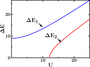
Figure 3: The energy gaps of a pair of quasi-particle and quasi-hole, $\Delta E_{1}$ and $\Delta E_{2}$ via $U$ when $n=1$ and $\mu=1$. One can see that MI-SF transition occurs at $U=12.15t$. At MI-SF transition, $\Delta E_{1}$ is still finite while $\Delta E_{2}$ close at the critical point. Hence the MI-SF transition is determined by $\Delta E_{2}$.

Solve Eq (51) and Eq (55), we can get the quasi-particle, quasi-hole spectra,

$$\hbar\omega_{1,qp} =\frac{1}{2}\left[-2\mu+(2n-1)U-\frac{1}{f_{\omega m+}^{2}}+\Delta E_{1,\mathbf{k}}\right]\ ,$$

$$\hbar\omega_{1,qh} =\frac{1}{2}\left[-2\mu+(2n-1)U-\frac{1}{f_{\omega m+}^{2}}-\Delta E_{1,\mathbf{k}}\right]\ ,$$

$$\hbar\omega_{2,qp} =\frac{1}{2}\left[-2\mu+(2n-1)U-\frac{1}{f_{\omega m-}^{2}}+\Delta E_{2,\mathbf{k}}\right]\ ,$$ (56)

$$\hbar\omega_{2,qh} =\frac{1}{2}\left[-2\mu+(2n-1)U-\frac{1}{f_{\omega m-}^{2}}-\Delta E_{2,\mathbf{k}}\right]\ ,$$

where

$$\Delta E_{1,\mathbf{k}} =\hbar\omega_{1,qp}-\hbar\omega_{1,qh}=\sqrt{U^{2}-\frac{(4n+2)U}{f_{\omega m+}}+\frac{1}{f_{\omega m+}^{2}}}\ ,$$ (57)

$$\Delta E_{2,\mathbf{k}} =\hbar\omega_{2,qp}-\hbar\omega_{2,qh}=\sqrt{U^{2}-\frac{(4n+2)U}{f_{\omega m-}}+\frac{1}{f_{\omega m-}^{2}}}\ ,$$ (58)

$$f_{\omega m\pm} =\frac{\mathcal{A}+\mathcal{B}\pm\sqrt{(\mathcal{A}-\mathcal{B})^{2}+4\mathcal{C}^{\ast}\mathcal{C}}}{2(\mathcal{A}\mathcal{B}-\mathcal{C}^{\ast}\mathcal{C})}\ .$$ (59)

Hence $\Delta E_{1/2,\mathbf{k}}$ are the dispersion of elementary excitations - a pair of quasi-particle and quasi-hole.

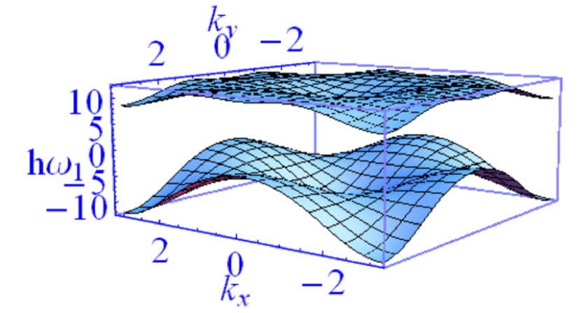
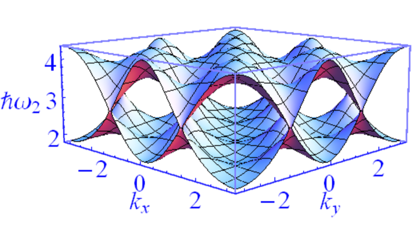
Figure 4: The spectra of quasi-particle and quasi-hole for the case of critical point, $U\approx 12.15\left|t\right|$ when $n=1$ and $\mu=1$. The upper one is for $\hbar\omega_{1,qp,qh}$ while the lower one is for $\hbar\omega_{2,qp,qh}$.

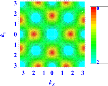
Figure 5: The dispersion of a pair of quasi-particle and quasi-hole $\Delta E_{2,\mathbf{k}}$ at the critical point with $U\approx 12.15\left|t\right|$ when $n=1$ and $\mu=1$.

From the information of quasi-particle-quasi-hole spectra, we can determine the phase boundary of MI-SF transition. We plot the energy gaps via $U$ in Fig3 with suitable $\mathbf{k}$ where the energy gaps take their maximum value, $\Delta E_{1/2}=\hbar\omega_{1/2,qp}-\hbar\omega_{1/2,qh}$. The MI-SF transition occurs at $U=U_{c}\approx 12.15\left|t\right|$ when the energy gap vanishes, which implies that $\Delta=\Delta E_{2}=0$. From the results, we found that the topologically nontrivial flat-band only lightly changes the phase boundary between superfluid phase and Mott phase.

In Fig.4, we plot the spectra of two branches of quasi-particle and quasi-hole, $\hbar\omega_{1,qp,qh}$ and $\hbar\omega_{2,qp,qh}.$ One can see that in MI phase, the dispersion of a pair of quasi-particle and quasi-hole $\Delta E_{1,\mathbf{k}}=\hbar\omega_{1,qp}-\hbar\omega_{1,qh}$ are always have larger energy than $\Delta E_{2,\mathbf{k}}=\hbar\omega_{2,qp}-\hbar\omega_{2,qh}$. Thus we focus on the quasi-particle-quasi-hole excitations with dispersion $\Delta E_{2,\mathbf{k}}$ in the following parts. For this case ($U=U_{c}\approx 12.15\left|t\right|$), the dispersion relation of the two quasi-particle quasi-hole spectra $\Delta E_{2,\mathbf{k}}$ is displayed in Fig.5. At MI-SF transition we found that the dispersion of quasi-particles and quasi-holes $\Delta E_{2,\mathbf{k}}$ show nodal-like behavior near special points in momentum space at $\mathbf{k}=(0,\pm\pi/2)$, $\mathbf{k}=(\pm\pi/2,0)$.

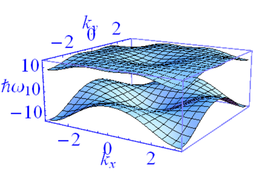
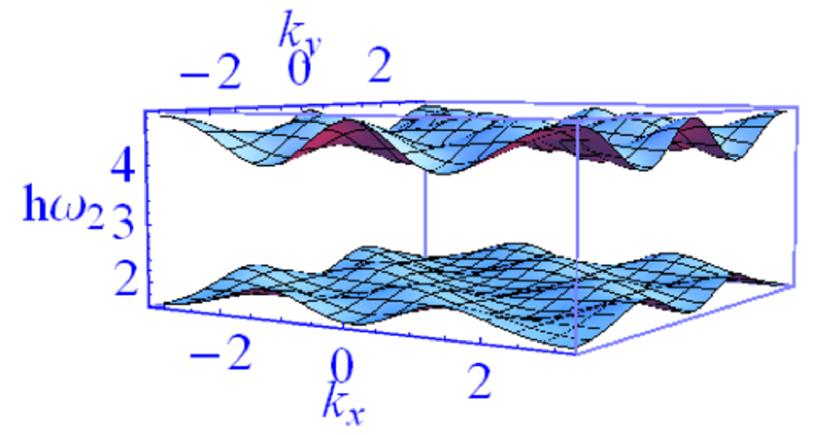
Figure 6: The spectra of quasi-particle and quasi-hole for the case of $U=12.5\left|t\right|$ when $n=1$ and $\mu=1$. The upper one is for $\hbar\omega_{1,qp,qh}$ while the lower one is for $\hbar\omega_{2,qp,qh}$.

In MI region, near MI-SF transition we also plot the spectra of two branches of quasi-particle and quasi-hole, $\hbar\omega_{1,qp,qh}$ and $\hbar\omega_{2,qp,qh}$ for the case of $U=12.5\left|t\right|$ in Fig.6. In addition, the dispersion of a pair of quasi-particle and quasi-hole is shown in Fig.7, from which we found that the quasi-particle-quasi-hole excitations have energy gap and the dispersion of a pair of quasi-particle and quasi-hole $\Delta E_{2,\mathbf{k}}$ becomes flat. To illustrate this effect, we calculate the flatness ratio, $\rho=\Delta/W$ where $W$ is the band width of the energy spectra and $\Delta$ is the energy gap of of the excitations. The flatness ratio $\rho$ for $U=12.5\left|t\right|$ is about $1.8$.

In MI region, far from MI-SF transition, we plot the spectra of two branches of quasi-particle and quasi-hole $\hbar\omega_{1,qp,qh}$ and $\hbar\omega_{2,qp,qh}$ and the dispersion for this case of $U=16\left|t\right|$ in Fig.8 and Fig.9, respectively. In this figure, we can see that there exists a flat-band of $\Delta E_{2,\mathbf{k}}$ obviously. Now the flatness ratio $\rho$ for $U=12.5\left|t\right|$ is about $16$.

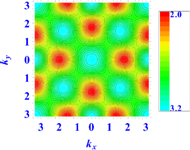
Figure 7: The dispersion of the quasi-particle quasi-hole $\Delta E_{2,\mathbf{k}}$ for $U=12.5\left|t\right|$ when $n=1$ and $\mu=1$.

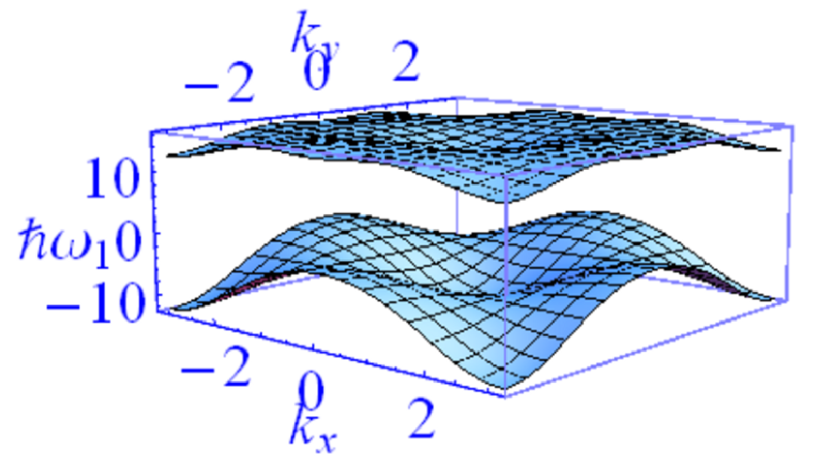
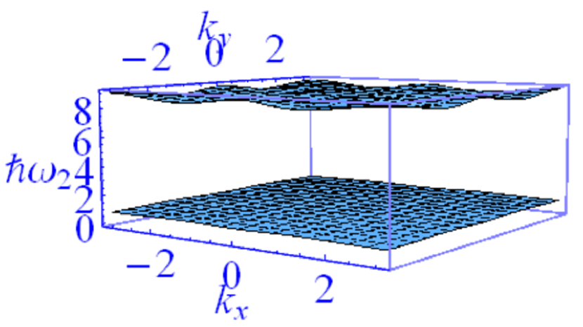
Figure 8: The spectra of quasi-particle and quasi-hole for the case of $U=16\left|t\right|$ when $n=1$ and $\mu=1$. The upper one is for $\hbar\omega_{1,qp,qh}$ while the lower one is for $\hbar\omega_{2,qp,qh}$.

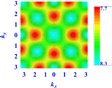
Figure 9: The dispersion of a pair of quasi-particle and quasi-hole $\Delta E_{2,\mathbf{k}}$ for $U=16\left|t\right|$ when $n=1$ and $\mu=1$.

Above results indicate that the dispersion of a pair of quasi-particle and quasi-hole will become more and more flat when we increase interaction strength, $U$. In Fig10, we displayed the inverse of flatness ratio $\rho$ via $U$ of generalized Bose-Hubbard on a checkerboard model with topologically nontrivial flat-band. From these results, we can see that the flatness ratio of the generalized Bose-Hubbard on a checkerboard model with topologically nontrivial flat-band increases with increasing of the interaction strength. On the other hand, we also calculate the flatness ratio of traditional Bose-Hubbard model. See blue line in Fig.10. From it we can see that the flatness ratio of traditional Bose-Hubbard model changes much more slowly than the flat-band model with increasing of the interaction strength. In this sense we can say that in MI phase, there indeed exist flat bands for (bosonic) quasi-particle or quasi-hole for the generalized Bose-Hubbard on a checkerboard model with topologically nontrivial flat-band.

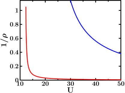
Figure 10: The inverse of flatness ratio $1/\rho$ via $U/\left|t\right|$ when $n=1$ and $\mu=1$, where the red line is that of flat-band model while blue line is that of traditional Bose-Hubbard model. One can see that flatness ratio of the generalized Bose-Hubbard on a checkerboard model with topologically nontrivial flat-band increases much more rapidly, implying that there exists flat-band for the bosonic excitations.

V Conclusion

In this paper, using a decoupling approximation, we studied the generalized Bose-Hubbard on a checkerboard model with topologically nontrivial flat-band in the mean-field level. We find that the MI-SF phase transition of the flat-band case only lightly changes compared with the traditional Bose-Hubbard model. We also calculate dispersion relations of the collective modes Mott phase. The results show that in MI phase the (bosonic) quasi-particle or quasi-hole also has flat bands. In the end, we should point out that until now we have no idea about how to realize this bosonic checkerboard model of flat-band in optical lattice of cold atoms. In the future we will revisit this issue and find way to realize this bosonic checkerboard model of flat-band with particular big nearest-neighbor (NN) and the next-nearest-neighbor (NNN) hoppings.

- (1) D. Jaksch, C. Bruder, J.I. Cirac, C. W. Gardiner, and P. Zoller, Phys. Rev. Lett. 81, 3108 (1998).
- (2) M. Greiner, O. Mandel, T. Esslinger, T. W. Hänsch, and I. Bloch, Nature 415, 39 (2002).
- (3) I. Buluta and F. Nori, Science 326, 108 (2009).
- (4) M. P. A. Fisher, P. B. Weichman, G. Grinstein, and D. S. Fisher, Phys. Rev. B 40, 546 (1989).
- (5) F. D. M. Haldane, Phys. Rev. Lett. 61, 2015 (1988).
- (6) E. Tang, J.-W. Mei, and X.-G. Wen, Phys. Rev. Lett. 106 236802 (2011).
- (7) K. Sun, Z. C. Gu, H. Katsura, and S. Das Sarma, Phys. Rev. Lett. 106, 236803 (2011).
- (8) T. Neupert, L. Santos, C. Chamon, and C. Murdy, Phys. Rev. Lett. 106, 236804 (2011).
- (9) Y.-F. Wang, Z.-C. Gu, C.-D Gong and D. N. Sheng, Phys. Rev. Lett. 107, 146803 (2011).
- (10) D. van Oosten, P. van der Straten, and H. T. C. Stoof, Phys. Rev. A 63, 053601 (2001).
- (11) L.-K. Lim, A. Hemmerich, and C. M. Smith, Phys. Rev. A 81, 023404 (2010).