Long-range interactions between substitutional nitrogen dopants in graphene: electronic properties calculations

Abstract

Being a true two-dimensional crystal, graphene has special properties. In particular, a point-like defect in graphene may induce perturbations in the long range. This characteristic questions the validity of using a supercell geometry in an attempt to explore the properties of an isolated defect. Still, this approach is often used in ab-initio electronic structure calculations, for instance. How does this approach converge with the size of the supercell is generally not tackled for the obvious reason of keeping the computational load to an affordable level. The present paper addresses the problem of substitutional nitrogen doping of graphene. DFT calculations have been performed for $9\times 9$ and $10\times 10$ supercells. Although these calculations correspond to N concentrations that differ by $\sim 10$%, the local densities of states on and around the defects are found to depend significantly on the supercell size. Fitting the DFT results by a tight-binding Hamiltonian makes it possible to explore the effects of a random distribution of the substitutional N atoms, in the case of finite concentrations, and to approach the case of an isolated impurity when the concentration vanishes. The tight-binding Hamiltonian is used to calculate the STM image of graphene around an isolated N atom. STM images are also calculated for graphene doped with 0.5 at% concentration of nitrogen. The results are discussed in the light of recent experimental data and the conclusions of the calculations are extended to other point defects in graphene.

I Introduction

Local defects and chemical doping is a well-documented way to tune the electronic properties of graphene. Niyogi2011 More specifically, the benefits of doping have been underlined in the context of (bio)sensing, Wang2010 lithium incorporation battery, Reddy2010 ; Li2012 and in other fields. Nitrogen (N) is a natural substitute for carbon in the honeycomb structure due to both its ability to form sp² bonds and its pentavalent character. It is not a surprise, then, that many publications deal with the production of N-doped graphene realized either by direct growth of modified layers Zhao2011 ; Wei2009 or by post-synthesis treatments. Guo2010 ; Joucken2012 Doping single-wall carbon nanotubes has also been considered. Arenal2010 ; Ayala2010 ; Lin2011

Recent STM-STS experiments of N-doped graphene Zhao2011 ; Joucken2012 have demonstrated the occurrence of chemical substitution. These experiments provide us with a detailed and local analysis with sub-atomic resolution of the electronic properties of the doped material. The STM images display a pattern having three-fold symmetry around the N atoms and having a strong signal on the C atoms bonded to the dopant, which ab-initio simulations reproduce well. Zheng2010 STS measurements have revealed a broad resonant electronic state around the dopant position and located at an energy of 0.5 eV above the Fermi level. Joucken2012

It is important to understand the effects of local defects and chemical doping on the global electronic properties of graphene, on its quantum transport properties and on its local chemical reactivity. It is the reason why the electronic properties of graphene doped with nitrogen have been investigated by several groups, mainly on the basis of ab-initio DFT techniques. Latil2004 ; Adessi2006 ; Lherbier2008 ; Zheng2010 ; Zhao2011 ; Fujimoto2011 ; Brito2012 The central advantage of the ab-initio approach is to be parameter free. A disadvantage is to be restricted to periodic systems as long as fast Fourier transforms need to be used to link direct and reciprocal spaces. In most instances, doping is therefore addressed in a supercell geometry that precludes the study of low doping concentration or disorder. In the case of single-wall carbon nanotubes, however, the electronic properties of isolated defects have been studied by first-principle methods based on scattering theory. Choi2000 For a nitrogen impurity in the (10,10) armchair nanotube, the local density of states on the N atom shows a broad peak centered at 0.53 eV above the Fermi level. The charge density associated with that quasi-bound state (donor level in the language of semiconductor physics) extends up to $\sim$1 nm away from the defect. This means that N atoms located $\sim$2 nm apart can interact, which requires examining with care the intrinsic validity of a supercell method.

The present work, based on both ab-initio DFT and semi-empirical tight-binding electronic structure calculations, aims at looking for interference effects generated by a distribution of N dopants in graphene as compared to the case of an individual impurity. We resort to different tight-binding parametrization strategies. The simplest one, based on just one adjustable parameter related to the defect, permits analytical calculations of the impurity levels. This model is described in Appendix A. We favor a more realistic approach, in which the perturbation induced by the defect is allowed to extend on the neighboring sites. This latter model is used to study the effects of disorder on the local and global electronic properties of doped graphene and to calculate STM images that we compare with available experimental data. The calculations and discussions are developed here for substitutional nitrogen. The conclusions would be qualitatively the same for boron doping and for other types of point-like defects.

II Methodology

The SIESTA package SanchezPortal1997 was used for the ab-initio DFT calculations. The description of the valence electrons was based on localized pseudo-atomic orbitals with a double-$\zeta$ polarization (DZP). Artacho1999 Exchange-correlation effects were handled within local density approximation (LDA) as proposed by Perdew and Zunger. Perdew1981 Core electrons were replaced by nonlocal norm-conserving pseudopotentials. Troullier1991 Following previous studies, Zheng2010 ; Joucken2012 the first Brillouin zone (BZ) was sampled with a $15\times 15$ grid generated according to the Monkhorst-Pack scheme Monkhorst1976 in order to ensure a good convergence of the self-consistent electronic density calculations. Real-space integration was performed on a regular grid corresponding to a plane-wave cutoff around 300 Ry. All the atomic structures of self-supported doped graphene have been relaxed.

As mentioned above, the DFT calculations are based on a code that requires a periodic system. As a consequence, a supercell scheme was adopted to handle substitutionaly doped graphene. The atomic concentration of dopants is then directly related to the size of the supercell: 0.6 at% for a $9\times 9$ supercell and 0.5 at% for a $10\times 10$ supercell.

For the tight-binding parametrization, the following, well-established procedure was followed. Latil2004 ; Adessi2006 ; Lherbier2008 The Hamiltonian included the $\pi$ electrons only, the hopping parameter between nearest-neighbor atoms was set to the ab-initio DFT value $\gamma_{0}$ = -2.72 eV. The same hopping was used between the N atom and its C first neighbors, which is not a severe approximation. It is indeed shown in Appendix A that a non-diagonal perturbation of the Hamiltonian can be offset by a renormalization of the N on-site energy, and this energy is a free parameter to be adjusted to the results of the ab-initio calculations. The C on-site energies were assumed to vary with the distance $d$ to the impurity according to a Gaussian law:

$$\varepsilon(d)=\varepsilon_{C}-|U|\,\exp(-0.5d^{2}/\sigma^{2})$$ (1)

where $|U|$ is the depth of the potential well induced by the nitrogen (boron induces a potential hump, instead Latil2004 ; Khalfoun2010 ) and $\varepsilon_{C}$ is the asymptotic bulk value of the on-site parameter of carbon. $\varepsilon_{C}$ defines the Dirac energy of pure graphene and has no other influence on the density of states (DOS) than a systematic shift of all the electronic levels. The standard deviation $\sigma$ in eq. (1) was set to 0.15 nm, according to data of Ref. [Khalfoun2010, ], whereas $U$ was chosen so as to best fit DFT local DOS calculated on the N atom in the $9\times 9$ supercell (see below).

In order to avoid the constraints of a periodic tight-binding Hamiltonian, the local DOS have been computed with the recursion method. Haydock1975 150 pairs of recursion coefficients were calculated and extrapolated to their asymptotic values related to the edges $\varepsilon_{C}\pm 3\gamma_{0}$ of the $\pi$ bands of pure graphene. It is worth emphasizing that this procedure avoids to introduce any broadening of the energy levels. A drawback is the presence of wiggles that may be observed in some densities of states. They are sorts of Gibbs oscillations generated by the Van Hove singularities, in particular by the abrupt discontinuities of the graphene $\pi$ DOS at both band edges.

III Periodic distribution of N

Fig. 1(a) shows DFT local densities of states on the N atom, on the first-neighbor atoms (C1) and on carbons located farther (0.5 – 0.7 nm) away (bulk), in a $9\times 9$ supercell. A broadening of 0.05 eV on a $45\times 45$ grid was used for the calculations. The important observation is the existence of two peaks, located at 0.55 and 0.92 eV above the minimum of the density of states in the N local DOS. Joucken2012

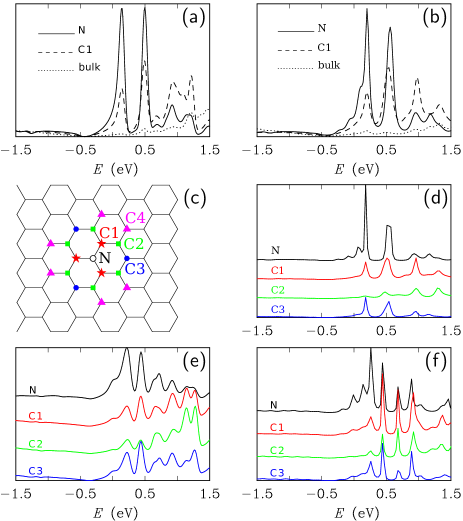
Figure 1: (a) DFT and (b) $\pi$ tight-binding local densities of states (LDOS) of graphene doped with nitrogen at a concentration of one impurity per $9\times 9$ supercell (162 atoms). The different curves represent the local DOS on the N atom, on the first-neighbor carbons (C1), and on a few distant carbons (bulk). (c) Labels assigned to the nitrogen dopant (N) and its first, second, third, and fourth neighbors (C1, C2, C3, and C4). (d) Tight-binding LDOS of the $9\times 9$ superstructure (same as in panel b) without energy broadening. (e) DFT and (f) tight-binding LDOS on and around a substitutional N atom in graphene with $10\times 10$ periodic distribution (200 atoms per cell). The curves, shifted vertically for clarity, correspond to the atomic sites N, C1, C2, and C3 shown in panel (c). For all LDOS curve plotted in this figure, the zero energy corresponds to the Fermi level.

The present DFT calculations are in overall good agreement with results published for $4\times 4$, Latil2004 ; Fujimoto2011 $5\times 5$, Brito2012 $7\times 7$, Zhao2011 and $10\times 10$ supercells. Zheng2010 The double-peak structure in the unoccupied part of the local N DOS plotted in Fig. 1(a)) was not observed in previous calculations due to the large energy broadening that was used there, Zheng2010 ; Zhao2011 except in Ref. [Joucken2012, ]. It will be demonstrated below that the observed double-peak structure is a consequence of long-range interactions between the N impurities that were reproduced periodically in the graphene sheet because of the supercell geometry.

Fig. 1(b) shows tight-binding densities of states of the same $9\times 9$ supercell after Lorentzian broadening aimed at facilitating the comparison with the DFT results. The latter are qualitatively well reproduced by the $\pi$-electron tight-binding Hamiltonian by taking $|U|$ = 4 eV in eq. (1). The present work aims at tailoring a simple tool for exploring the effects of the defect configurations. For that reason, achieving the best possible fit of DFT calculations for a specific supercell is superfluous. By comparison, the on-site energies in Ref. [Adessi2006, ] can be approximated by a sum of two Gaussians, $\varepsilon(d)=\varepsilon_{C}-2.95\,\exp(-0.5d^{2}/\sigma_{1}^{2})-0.59\,\exp(-0.5d^{2}/\sigma_{2}^{2})$ (in eV), with $\sigma_{1}$ = 0.10 nm and $\sigma_{2}$ = 0.39 nm. The second term has a longer range than the single Gaussian law used in the present calculations, and the potential well at the N location is about 10% shallower than here.

The tight-binding densities of states of the same $9\times 9$ superstructure, now calculated without energy broadening, are displayed in Fig. 1(d). A substructure clearly emerges where the broadened local DOS only showed the double-peak feature discussed here above. In addition, Fig. 1(d) reveals that there are much less electronic states in the region between 0 and 1.5 eV on the second-neighbor atoms (C2) than on the first- (C1) and third-neighbor (C3) carbons (see Fig 1(c) for the notations). The same observation as for C2 can be made for the local DOS on the fourth neighbors (not shown). This alternation between lower and higher densities of states brings out the fact that the two sublattices of graphene are differently affected by a substitutional defect (see Appendix A).

The reliability of the tight-binding calculations compared to DFT can be appreciated from Figs. 1(e,f) obtained for a $10\times 10$ supercell (0.5 at% concentration of N). The good agreement between the two approaches reinforces the fact that the parametrization of the tight-binding on-site energies used for the $9\times 9$ supercell describes well the doped graphene systems and does not require further adjustment depending on the actual concentration. Electronic states localized on and near the N dopant are observed within 1.5 eV from the Dirac energy, as for the $9\times 9$ supercell. However, the multi-peak structure in the local N DOS of $10\times 10$ (Fig. 1(f)) is totally different from that of $9\times 9$ (Fig. 1(d)), despite similar N concentrations (0.5 at% and 0.6 at%, respectively). This finding is a clear indication of the importance of interference effects among the supercells.

The band structures of the DFT calculations shown in Fig. 2 provide us with another difference between the two superstructures: the $10\times 10$ N-doped superstructure has a direct band gap of $\sim$0.05 eV at the $K$ point of its Brillouin zone, whereas the $9\times 9$ N-doped superstructure has no gap. Symmetry considerations and arguments from perturbation theory developed in Appendix B explain why it is so. The $K$ and $K^{\prime}$ points of graphene move to the $K$ and $K^{\prime}$ points of the folded Brillouin zone of a $p\times p$ supercell when $p$ is not divisible by 3, whereas they are both mapped onto the $\Gamma$ point when $p$ is an integer multiple of 3. Martinazz2010 In the latter case, the fourfold degeneracy of the Dirac energy at the $\Gamma$ point of a supercell of pure graphene is partly lifted by the perturbation brought about by the N atoms. As demonstrated in Appendix B, there remain $\pi$ and $\pi^{*}$ bands that cross the Dirac energy at $\Gamma$. This crossing as clearly visible in Fig. 2(a) for the $9\times 9$ superstructure, which therefore has no gap. In direct space, a doped superstructure has point group symmetry $D_{3h}$. The symmetry of the $\Gamma$ point of the superstructure, $D_{3h}$, which is the same as that of the $K$ and $K^{\prime}$ points of pure graphene, Malard2009 ; Kogan2012 has irreducible representations of dimension one and two. A twofold degeneracy of some electron energy bands is therefore allowed at the zone center of a doped superstructure. By contrast, this degeneracy is forbidden at the $K$ and $K^{\prime}$ points of the folded zone because the symmetry of theses points, from $D_{3h}$ in pure graphene, is reduced to $C_{3h}$ in the doped superstructure. The latter point group has only one-dimensional irreducible representations. As a consequence, the crossing of $\pi$ and $\pi^{*}$ bands is symmetry forbidden at $K$ and $K^{\prime}$. A periodic substitution of N for C therefore opens a gap in these $p\times p$ supercells for which $p$ is not divisible by 3, as shown in Fig. 2(b) for the $10\times 10$ superstructure. It is demonstrated in Appendix B that the band gap in those superstructures scales with $p$ like $E_{g}\approx V/p^{2}$, where $V$ is of the order of 10 eV. Other local gaps of the order of $V/p^{2}$ appear in the band structures of Figs. 2(a,b) at the edges of the folded Brillouin zone. They produce pseudo-gaps and sub-peaks in the densities of states clearly discernible in Fig. 1 for both the $9\times 9$ and $10\times 10$ superstructures. As a result, supercells of the order of $30\times 30$ at least would be necessary to reproduce the characteristic features of an isolated impurity with an energy resolution better than $0.01$ eV.

In the tight-binding calculations, the band gap of the $10\times 10$ superstructure is located 0.14 eV below the Dirac point of pure graphene ($\varepsilon_{C}$). The Fermi level $E_{F}$ of the doped superstructures was found to lie 0.27 eV and 0.25 eV above $\varepsilon_{C}$ for the $9\times 9$ and $10\times 10$ systems, respectively, which means 0.43 eV and 0.39 eV above the minimum of the DOS (the corresponding DFT values are 0.42 and 0.36 eV, respectively). The $\sigma$ bands below the Fermi energy are completely filled, the $\pi$ bands of the supercell must accommodate an extra electron brought about by the nitrogen. The occupied local $\pi$ DOS of the N atom contains 1.36 electron in both the $9\times 9$ and $10\times 10$ supercells. The remaining 0.64 excess electron is distributed on the surrounding carbons, of which a total of 0.56 sits on the three first neighbors (C1), which are therefore negatively charged.

For both $9\times 9$ and $10\times 10$ doped supercells, there is a localized state expelled from the $\pi$ band and located 9.35 eV below $E_{F}$, to be compared with 8.65 eV in DFT calculations. This localized state weights more than 25% (0.57 state of the N local DOS, which can accommodate 2 electrons including the spin degeneracy). The large value of the weight can be understood from the arguments developed in Appendix A for a simplified tight-binding Hamiltonian.

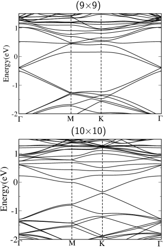
Figure 2: DFT band structures of the $9\times 9$ (top) and $10\times 10$ (bottom) N-doped superstructures shown along the high-symmetry lines of their first Brillouin zone. The zero of energy coincides with the Fermi level.

We conclude here that the supercell technique would require very large supercells (up to $30\times 30$) if it were desired to describe the electronic states of an isolated defect. In other words, the supercell technique is badly convergent when the size of the cell increases, particularly in low dimensions. The corresponding long range of a local perturbation produces interferences between the images of the defect generated by the periodic boundary conditions (see also Ref. [Zanolli2010, ]).

IV Isolated N impurity

We now turn our attention to the case of an isolated N impurity studied by tight-binding. The local DOS on and around an isolated N impurity are presented in Fig. 3. The calculations were performed on a 150x150 cell of graphene (45,000 atoms) with periodic boundary conditions. By restricting the number of pairs of recursion coefficients to 150, the impurities located in adjacent cells do not feel each other, which means that the N atoms are virtually isolated. In the N local DOS, there is a tall asymmetric peak located 0.5 eV above the Dirac energy ($\varepsilon_{C}$) of graphene which coincides here with the Fermi level. The peak broadens and shifts to 1 eV on the first neighbors and moves up further to 1.5 eV on the second neighbors. The local DOS on the third-neighbor atoms reproduces the resonance peak of the impurity, with a smaller amplitude. The local DOS on the fourth neighbors (not shown) bears resemblance with that of pure graphene. It is interesting to observe in Fig. 3 that there remains almost nothing of the Van Hove singularities of graphene at $\varepsilon_{C}\pm\gamma_{0}$ on the N and C1 sites.

Figure 3: Tight-binding local $\pi$ densities of states on and around an isolated impurity in graphene. The labels correspond to the defect site (N), the first, second and third neighbors (C1, C2 and C3). The curves have been shifted vertically for clarity. The zero of energy is $\varepsilon_{C}$.

The problem of an isolated impurity in graphene can be addressed analytically if one simplifies the Hamiltonian to a point-like defect by ignoring the Gaussian delocalization of the perturbation ($\sigma\to 0$ in eq. (1)). Details are presented in Appendix A. If this simple model captures the essential physics of the problem, it fails in producing all the details set up by the delocalized nature of the perturbation. As shown in the Appendix A, perturbing the first-neighbor C atoms, in addition of course to the substitution site, leads to a better picture.

V Randomly distributed N atoms

Experimentally, nitrogen doping of graphene leads to randomly distributed substitutional sites, Zhao2011 ; Joucken2012 with perhaps some preference of the dopant atoms to sit on the same sublattice, at least locally. Zhao2011 The calculations illustrated in the present Section were performed for nitrogen distributed randomly with an atomic concentration of 0.5%, identical to that realized with the $10\times 10$ superstructure. The selection of the substitutional sites was constrained by the requirement that the distance between two nitrogens remains larger than 12$\sigma$ = 1.8 nm (see eq. (1)). The reason for that was to avoid any overlapping of the potential wells generated by the dopants.

Fig. 4 shows a configurational averaging of the local densities of states when the N atoms have equal probabilities to sit on one or the other of the graphene sublattices. This case will be referred to as “unpolarized” (or “uncompensated”).Pereira2008 By configurational averaging, it is meant the arithmetic average of local DOS on 50 nitrogens selected randomly — among the 225 dopant atoms that the 150x150 sample box contains — and the arithmetic average of local DOS on 150 randomly-selected C1, C2 and C3 sites. The N, C1, C2, and C3 average local DOS for the unpolarized disordered distribution all have a remarkable similarity with the ones obtained for an isolated impurity (Fig. 3). The result are in agreement with N local DOS for randomly distributed impurities obtained by Lherbier et al. Lherbier2008 with a small broadening.

Figure 4: Configurational average of the local $\pi$ densities of states on and around substitutional N atoms in a graphene sheet containing 0.5 at% of nitrogen atoms randomly distributed on the two sublattices. The labels correspond to the nitrogen dopant (N), the first, second and third neighbors (C1, C2 and C3). The curves have been shifted vertically for clarity. The zero of energy is $\varepsilon_{C}$.

When the N atoms are put, still randomly, on the same sublattice (“polarized” case”), the multi-peak structure characteristics of the superlattice (see Fig. 1(e,f)) reappear on the average local DOS shown in Fig. 5. Interestingly, the local DOS on the second-neighbor atoms (C2), which belongs to the same sublattice as the N atom they surround, are virtually the same in Figs. 4 and 5, insensitive to the polarization of the N distribution. It is also interesting to remark that, like with the $10\times 10$ superstructure, there is a tiny gap of states 0.1 eV below the Dirac energy. The gap looks narrower in case of the unpolarized distribution compared to the polarized one. In the polarized case, the appearance of a gap is natural since the average diagonal potential breaks the symmetry between the two sublattices. Similar effects have been observed in the case of vacancies.Pereira2008

Figure 5: Configurational average of the local $\pi$ densities of states on and around substitutional N atoms in a graphene sheet containing 0.5 at% of nitrogen atoms randomly distributed on the same sublattice. The labels correspond to the nitrogen dopant (N), the first, second and third neighbors (C1, C2 and C3). The curves have been shifted vertically for clarity. The zero of energy is $\varepsilon_{C}$.

Averaging the local densities of states makes visible the distinction between unpolarized and polarized distributions of N. However, for a given configuration of the dopant atoms, the local DOS varies from site to site. How much that variation can be is illustrated in Fig. 6, which compares local DOS calculated on three different N atoms for both the unpolarized and the polarized distributions. The variations from site to site are so important that the local DOS is not a reliable indicator of the global distribution of the nitrogen atoms among the two sublattices. If it is true that the N local DOS displayed in Fig. 6 are less peaked that the N local DOS of the $10\times 10$ superstructure (Fig 1(e,f)), identifying which is which would be difficult on the experimental side if one had only STS spectra to deal with.

Figure 6: Local DOS on three N atoms randomly selected in graphene doped at concentration 0.5 at%. The unpolarized case (left) refers to dopants located on the two sublattices, whereas the dopants all sit on the same sublattice in the polarized case (right). The zero of energy is $\varepsilon_{C}$.

Finally, it may be important to remark that the minimum of the $\pi$ density of states around the N dopants does not coincide with the atomic level $\epsilon_{C}$ of carbon in graphene (the Dirac point energy; see also Refs. [Pereira2008, , Skrypnyk2009, , Wu2008, ]). Depending on the concentration, the DOS minimum shifts slightly below $\epsilon_{C}$ (see e.g. Figs. 4 and  5).

VI STM images

A reliable information on the electronic structure of doped graphene can be obtained by STM imaging. A tip polarized negatively compared to the graphene layer probes the unoccupied states where a N substitutional impurity and the adjacent carbon atoms have peaks in their local DOS. The increase of electronic density of states, compared to graphene, in this energy region gives rise to a bright triangular spot in the STM image, Zheng2010 ; Zhao2011 ; Joucken2012 ; Brito2012 with two possible orientations with respect to the honeycomb lattice depending on the sublattice on which the N dopant sits. These two orientations are rotated by 180^∘ from each other, as observed experimentally.Zhao2011 ; Joucken2012

Fig. 7 is a tight-binding STM image Meunier1998 computed for graphene with a single N impurity. The prominent triangular arrow-head at the center of the image is located on the N, C1 and C3 sites. The second-neighbor carbons (C2) atoms do not participate much to the STM signature of the dopant. This is so because the local DOS in the energy window probed by the STM current (0 to 0.5 eV) is smaller on the C2 atoms than on the N, C1 and C3 atoms (see Fig. 3).

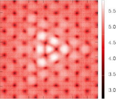
Figure 7: Tight-binding STM constant-current image of graphene with an isolated N impurity located near the center, computed for a negatively-polarized tip ($V_{\text{tip}}$ = -0.5 V). The vertical scale is the tip height (Å) above sample. The image size is 2 nm along both sides.

Fig. 8 shows two STM images computed for graphene doped with N at 0.5 at% concentration, the dopants being randomly distributed on the two sublattices. In the configuration shown in image (a), there are two impurities located 1.9 nm apart sitting on the same sublattice. The two nitrogens captured in images (b) do not sit on the same sublattice, which explains why the related triangular STM patterns are oriented differently. The scale used for the STM signal (tip height at constant current) is identical for both images. For improving the contrast, the scale has been saturated below 4.0 Å and above 5.8 Å. Two dopants interfere more when they are located on the two sublattices than when they sit on the same sublattice.

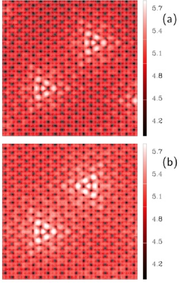
Figure 8: Constant-current STM images computed for two configurations of graphene doped with 0.5 at% N. The distribution of the N atoms is random. The two nitrogen atoms visible in image (a) lie on the same sublattice, which is not the case in image (b). In both cases, the STM tip is polarized at -0.5 V with respect to the sample. Each image is a square of 4 nm edge.

In tight-binding STM theory, Meunier1998 there is an empirical parameter coupling the tip apex to the sample atoms, which was chosen independent of the chemical nature of the probed atoms. In other words, the STM calculations differentiate a N atom from the C atoms only through intrinsic effects that the former has on the electronic structure of the doped graphene. In DFT calculations, the standard way to generate an STM image is via Tersoff-Hamann’s theory. Tersoff1983 In addition to local variations of the DOS, the tunnel current depends on the spatial extension of the $\pi$ orbitals in the direction perpendicular to the atomic plane. For doped graphene, the $2p_{z}$ orbital of N decreases more rapidly than the C $2p_{z}$ orbital does, Zheng2010 which means that the contrast of the computed image depends on the tip–sample distance. This dependence is illustrated in Figs. 9(a) and (b) that represent DFT constant-current STM images computed for a small current (large tip-sample distance) and for a large current (small tip-sample distance), respectively. The local DOS is larger on top of the N atom than on the top of all the other atoms, but it decreases much more rapidly in the normal direction. This explains the small brightness of the N site for the large tip–sample distance. Experimentally, variations of the STM contrast have also been observed as a function of the current/voltage conditions, Joucken2012 where image of the dopant atom protrudes in some occasions and does not in other occasions. It is tempting to attribute this observation to variations of the tip–sample distances depending on the current setpoint, as in Fig. 9. However, the experimental distance is much larger than the one that can be achieved numerically in DFT, due to the fast decay of the localized basis set when moving away from the sample surface.

Figure 9: DFT calculation of constant-current STM images of $10\times 10$ N-doped graphene for two levels of the tunnel current: (a) high and (b) low (see text). The tip bias polarization is -0.5 V, the vertical scale is the tip height (Å) above sample. Each image represents a square of 4 nm edge centered on a N dopant.

VII Conclusions

Tight-binding and DFT electronic calculations reveal that the perturbation induced by N dopants in graphene is long ranged. This is not a surprise when one remembers that the Green function of the free-electron problem in two dimensions is the Bessel-Hankel function of zeroth order $(i/4)H_{0}^{(1)}(k|\vec{r}-\vec{r}^{\prime}|)$, which slowly decreases like $1/\sqrt{kd}$ with the distance $d=|\vec{r}-\vec{r}^{\prime}|$, where $k=\sqrt{\hbar^{2}/2mE}$. For the $\pi$-electron tight-binding Hamiltonian on the honeycomb lattice, the Green function elements $G_{nm}^{0}$ can also be approximated, at low energy, by Hankel functions of $\delta k|\vec{r}_{m}-\vec{r}_{n}|$, now of order zero or one, depending on whether they refer to sites $m$ and $n$ located on the same sublattice or not.Wang2006 In this regime, the energy $E$ is linearly related to $\delta k$ by the dispersion relation $E=\hbar v_{F}\delta k$, where $v_{F}$ is the Fermi velocity, and the Hankel functions are also multiplied by the energy and by periodic functions describing $\sqrt{3}\times\sqrt{3}$ modulations related to the Dirac wave vectors $K$ and $K^{\prime}$. For large separation distances, the Green function elements decay slowly, like $1/\sqrt{E\;|\vec{r}_{m}-\vec{r}_{n}|/\hbar v_{F}}$, except for very small excitation energies where the Hankel functions diverge. A more detailed discussion will be given elsewhere. FD2012

The scattering formalism developed in Appendix A for the case of a point-like defect emphasizes the central role of the Green function in the understanding of the perturbation induced by the defect. Hence the long-range interaction between dopants in graphene. It is important to realize that this long-range interaction is not the consequence of using an extended perturbation of the on-site energies around the defect (eq. (1)). Things actually go the other way round: a defect perturbs the crystal potential far away, because of the slow decay of the scattering it produces. As a consequence, the parameters of the tight-binding Hamiltonian that mimic ab-initio calculations are affected in a sizable neighborhood of the defect. Adessi2006

This long-range interaction has several effects. First, it produces interferences between the duplicates of the defect generated by periodic boundary conditions when a supercell approach is used. The latter must therefore be used with caution. Second, substitutional impurities dispersed in graphene cannot be treated as independent defects as soon as the distance between two of them becomes too small, about 2 nm in the case of nitrogen. Increasing the strength of the local potential also increases the range of the perturbation it produces. This unusual behavior is actually related to the properties of the Green functions at low energy (see Appendix A and Refs. [Skrypnyk2009, , Skrypnyk2006, , Skrypnyk2011, ]). As mentioned in Appendix A, the deepest defect is the vacancy. Nitrogen, with its 10 eV effective perturbation parameter, is not a shallow defect. Boron would not be a shallow impurity either. B substitution can be described by a potential hump, instead of a well, with a similar $|U|$ as nitrogen and a similar long-range perturbation. Latil2004 ; Khalfoun2010 In the case of more complex defects, such as N plus vacancy, Hou2012 P plus N, Cruz2009 or O₃, Leconte2010 it would be more difficult to define local parameters and to assess the importance of long-range interactions along the same way as in this paper.

As demonstrated experimentally, the partition of the honeycomb network in two sublattices has subtle effects on STM image of graphene with substitutional impurities, as exemplified by Fig. 8. The STM image of a dopant in graphene may be influenced by the proximity of another dopant. This is a direct consequence of the defect interactions mediated by graphene. What happens when two impurities come very close to each other remains to be clarified. A new parametrization of the tight-binding Hamiltonian would be required if one had to obtain, from calculations, the STM topography of neighboring N dopants.

Acknowledgments This research has used resources of the Interuniversity Scientific Computing Facility located at the University of Namur, Belgium, which is supported by the F.R.S.-FNRS under convention No. 2.4617.07 and the FUNDP.

Appendix A. The impurity problem in graphene

In this Appendix, a simple but illustrative perturbation model is developed. It is assumed that the on-site energies all take the unperturbed bulk value $\varepsilon_{C}=0$, except on the nitrogen atom where $\varepsilon_{N}=U$. The tight-binding Hamiltonian can be set in the form:

$$H=H^{0}+V=-\sum_{n,m}|n\rangle t_{nm}\langle m|+|0\rangle U\langle 0|\;.$$ (2)

The states $|n\rangle$ denote $\pi$ orbitals centered on sites $n$: $\varphi_{\pi}(r-n)=\langle r|n\rangle$. $H^{0}$ is the usual tight-binding Hamiltonian where only hopping integrals $t_{nm}\equiv\gamma_{0}$ between first neighbors $n$ and $m$ are kept, and $V$ is the localized potential of the N atom at site $0$. The local density of states $n(r,E)$ is given by:

$$n(r,E)=\sum_{n,m}n_{nm}(E)\varphi_{\pi}(r-n)\varphi_{\pi}(r-m)\;,$$ (3)

where $n_{nm}(E)$ is obtained from the Green function or resolvent $G(z)=(z-H)^{-1}$:

$$n_{nm}(E)=\frac{-1}{\pi}\;\lim_{\varepsilon\to 0}\text{ Im }\langle n|G(E+i\varepsilon)|m\rangle\;.$$ (4)

$G(z)$ can then be calculated in terms of the unperturbed Green function $G^{0}(z)=(z-H^{0})^{-1}$; this is the so-called Koster-Slater-Lifshitz problem. If the matrix elements $\langle n|G(E+i\varepsilon)|m\rangle$ are written $G_{nm}(z)$, we have:

$$G_{nm}=G^{0}_{nm}+G^{0}_{n0}\tau G^{0}_{0m}\quad;\quad\tau=\frac{U}{1-UG^{0}_{00}}\;.$$ (5)

In particular, on the impurity site, we have $G_{00}=G^{0}_{00}/(1-UG^{0}_{00})$,KosterSlater1954 ; Lifshitz1965 and the local density of states on the N site, $n_{N}(E)\equiv n_{00}(E)$ is given by:

$$n_{N}(E)=\frac{n^{0}(E)}{(1-UF^{0}(E))^{2}+\pi^{2}U^{2}n^{0}(E)^{2}}\;,$$ (6)

where $F^{0}(E)$ is the real part of the Green function $G^{0}_{00}(E+i\varepsilon)$, i.e. the Hilbert transform of the unperturbed density of states of graphene $n^{0}(E)$.

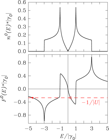
Figure 10: Real ($F^{0}(E)$) and imaginary ($n^{0}(E)$) parts of the Green function of the graphene $\pi$ tight-binding Hamiltonian along the real axis, in units of $|\gamma_{0}|$. The intersection of $F^{0}(E)$ with the reciprocal of the perturbed level $1/U$ (dashed line) in the vicinity of the Dirac point gives the energy $E_{r}$ at which the local DOS of the impurity has a resonance (open circle symbol). There is another intersection (filled symbol) giving rise to a localized state below the $\pi$-electron density of states.

Close to the Dirac point, $n^{0}(E)\sim|E|$ and $F^{0}(E)\sim E\ln|E|$, and provided $U$ is large enough, $n_{N}(E)$ shows a resonant behavior around the energy $E_{r}$ such that $(1-UF^{0}(E_{r}))=0$ (see the open-circle symbol in Fig. 10). This has been discussed in many places. Skrypnyk2006 ; Wang2006 ; Wehling2007 ; Pereira2008 ; Wu2008 ; Toyoda2010 ; Chang2011 It turns out that a value for $U$ of the order of $-10$ eV reproduces a resonance at the position obtained with the previous model (compare Fig. 11(a) with Fig. 3) instead of the value $U=-4$ eV in the previous approach. However, the shapes of the local DOS differ to some extent between the local-perturbation model developed in this Appendix and the more delocalized potential well considered throughout this paper. The resonance here (Fig. 11(a)) is weaker on the N site than on the sites C1 and C3 located on the other sublattice, which can be explained from the symmetry properties of the unperturbed Green functions: $G_{nm}(z)$ is and odd or even function of $z$ depending on whether the sites $n$ and $m$ belonging to the same sublattice of the graphene structure or not. As a consequence, for example, $G^{0}_{00}(z=0)=0$ whereas the real part of $G^{0}_{0n}(z=0)$ does not vanish when $n$ is a first neighbor, which has a big impact on the local densities of states (see eq. (5)). FD2012 Also the Van Hove singularities at 2.7 eV are still present here.

In addition to the resonant state located above the Dirac point, Fig. 10 reveals the existence of a localized state lying below the $\pi$-electron DOS, where the on-site perturbation level $1/U$ intersects the curve $F^{0}(E)$ at $-4.5|\gamma_{0}|$ (solid square symbol). The weight (residue) of this localized state is inversely proportional to the slope of $F^{0}(E)$ at the intersection. This is the localized state found at 9.35 eV below $E_{F}$ in tight-binding and 8.65 eV below $E_{F}$ in DFT calculations for the doped superstructures (Section III).

This one-parameter model can be generalized to other type of local defects or chemical doping. B doping, with a positive $U$, will yield results symmetrical to those obtained for N: it can indeed be anticipated from Fig. 10 that the resonance state will now appear near the top of the occupied states, as confirmed by DFT calculations. Zheng2010 ; Latil2004 ; Khalfoun2010 The limit $U\to\infty$ corresponds to the introduction of a vacancy instead of a substitutional impurity. Because of the vanishing of the density of states and of the logarithmic divergence of $F^{0}(E)$, this limit is singular and must been studied with special care.Pereira2008 ; Wu2008 ; Toyoda2010 ; Chang2011 ; Yuan2010 The resonant state becomes very narrow, but does not become a genuine bound state. The total density of states varies as $1/([\ln|E|]^{2}|E|)$ and the perturbation of the electronic density is concentrated on the first neighbors and on the sites belonging to the sublattice different from that of the vacancy.FD2012

The simple model developed here above allows one to address the question of the role of N-C hopping interactions on the local DOS on the impurity. When the N-C hopping takes a value $\gamma$ different from the one $\gamma_{0}$ between the C atoms, the Green function element on the perturbed site can be set in the form

$$G_{00}(z)=\frac{1}{z-U-(\gamma^{2}/\gamma_{0}^{2})\Sigma^{0}(z)}$$ (7)

where $\Sigma^{0}(z)$ is the self energy of the unperturbed graphene. In the notations of the above formalism, the self energy can be identified to $\Sigma^{0}(z)=z-1/G^{0}_{00}(z)$. Inserting this expression in the right-hand side of eq. (7) leads to a generalization of eq. (6) valid for $\gamma\neq\gamma_{0}$. In particular, the resonance condition in the vicinity of $E$ = 0 becomes

$$\frac{\gamma^{2}}{\gamma_{0}^{2}U+(\gamma^{2}-\gamma_{0}^{2})E_{r}}=F^{0}(E_{r})\;.$$ (8)

By comparison with the situation depicted in Fig. 10, the intersection of $F^{0}(E)$ needs now to be search for with a curve whose ordinate and slope at the origin are $-\gamma^{2}/(\gamma_{0}^{2}|U|)$ and $\gamma^{2}(\gamma_{0}^{2}-\gamma^{2})/(\gamma_{0}^{2}U)^{2}$, respectively. If $|\gamma|<|\gamma_{0}|$, which should be the case here since the N atom is smaller than the C one, the ordinate at the origin of the curve moves up and its slopes becomes positive. These two effects pull the resonant energy $E_{r}$ closer to the origin compared with the simplest situation where $|\gamma|=|\gamma_{0}|$. However, if the hopping perturbation is small, renormalizing the on-site level $U$ to a larger absolute value $U_{\text{eff}}$ would produce the same effect. This conclusion validates the approach used so far to not modifying the N-C hopping.

We have finally considered an intermediate model between the Gaussian distribution of the on-site energies and the one-parameter model just described. We took $U_{0}$ on the N site and a second perturbation potential $U_{1}$ on the first neighbors, with values fixed by eq. (1), $U_{0}=-4$ eV; $U_{1}=-2.57$ eV. The agreement with the full Gaussian model is much better than with the one parameter model (Fig. 11(b)). It is fairly remarkable to realize that the intensity of the resonance state on the N site increases when the potential is delocalized on the first neighbors.

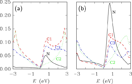
Figure 11: Local densities of states deduced from the simple tight-binding model for an isolated nitrogen impurity in graphene. (a) On-site perturbation energy $U$ = -10 eV on the N site only; (b) on-site perturbation on the N (-4 eV) and the three C1 sites (-2.57 eV).

Appendix B. Band gap opening in doped superstructures

The following perturbation theory is based on the same model Hamiltonian as in eq. (2), except that the potential $V$ refers now to the perturbation brought about by the periodic array of nitrogen atoms in substitution for C in a $p\times p$ supercell of graphene. These atoms occupy one among the $2N=2p^{2}$ sublattices of the supercell, here denoted sublattice $1$:

$$H=H^{0}+V=-\sum_{n,m}|n\rangle t_{nm}\langle m|+\sum_{n\in 1}|n\rangle U\langle n|\;.$$ (9)

When $V=0$, there are four states with zero energy (Dirac energy of the unperturbed graphene): $|K^{i}\rangle$ and $|K^{\prime i}\rangle$, where $i=A,B$ denote the sublattices of the graphene structure and $|K^{i}\rangle$, $|K^{\prime i}\rangle$ are the corresponding Bloch functions:

$$|K^{A(B)}\rangle=\frac{1}{\sqrt{N}}\sum_{n\in A(B)}e^{iK.n}|n\rangle\;.$$ (10)

where $K.n$ in the exponential represents the dot product of the wave vector of the $K$ point of graphene and the position vector of the site $n$ in real space.

It will be assumed that the sublattice $1$ is an $A$ sublattice. Then, the states $|K^{B}\rangle$ and $|K^{\prime B}\rangle$, having no amplitude on sublattice $1$, are eigenstates of zero energy for any value of the on-site perturbation $U$. Very close to zero energy, furthermore, only the ($(|K^{A}\rangle,|K^{\prime A}\rangle)$) subspace needs to be considered. In particular,

$$\langle K^{A}|V|K^{A}\rangle = \langle K^{\prime A}|V|K^{\prime A}\rangle=\frac{1}{N}\sum_{n\in 1}1=U/p^{2}$$ (11)

$$\langle K^{A}|V|K^{\prime A}\rangle = \frac{1}{N}\sum_{n\in 1}\exp[i(K^{\prime}-K).n]=U/p^{2}\,\delta_{K^{\prime}-K,G}\;,$$ (12)

where the Kronecker symbol imposes that $K^{\prime}-K$ be a vector of the reciprocal lattice of the supercell, i.e. it is one when $p=3q$ is a multiple integer of 3 and is $0$ if $p$ is not divisible by 3.

As a consequence, in the case $p=3q$, the four states with zero energy are mapped onto the zone center. Two of them, with non-zero amplitudes on the $B$ sites, remain degenerate with zero energy; the other two states have energy $E=0$ and $E=-2|U|/p^{2}$ to lowest order in perturbation. There are then two plus one states at zero energy, but this is an accidental degeneracy due to the simplified tight-binding model. When $p$ is not divisible by 3, the degeneracy at the $K$ and $K^{\prime}$ points of the folded zone is lifted: at each point, one state remains at zero energy ($|K^{B}\rangle$ or $|K^{\prime B}\rangle$, respectively) whereas the other state moves down at energy $-|U|/p^{2}$ to lowest order in perturbation.

All these features are clearly visible in the band structures of the $9\times 9$ and $10\times 10$ superlattices shown in Fig. 2. Since a realistic value for $|U|$ is about 10 eV, the gap for the $10\times 10$ case should be of the order of $10/p^{2}=0.1$ eV, not far from the actual value (see Section III). For the $9\times 9$ superstructure, the expected crossing between the two linear $\pi$ and $\pi^{*}$ bands is observed at the $\Gamma$ point close to two parabolic branches separated from each other by a gap about twice this value.

References

- (1) S. Niyogi, E. Bekyarova, J. Hong, S. Khizroev, C. Berger, W. de Heer, and R.C. Haddon, J. Phys. Chem. Lett. 2, 2487 (2011).
- (2) Y. Wang, Y. Shao, D.W. Matson, J. Li, and Y. Lin, ACS Nano 4, 1790 (2010).
- (3) A.L.M. Reddy, A. Srivastava, S.R. Gowda, H. Gullapall, M. Dubey, and P.M. Ajayan, ACS Nano 4, 6337 (2010).
- (4) Y. Li, J. Wang, X. Li, D. Geng, M.N. Banis, R. Li, and X. Sun, Electroch. Comm. 18, 12 (2012).
- (5) L. Zhao, Rui He, Kwang Taeg Rim, Th. Schiros, Keun Soo Kim, Hui Zhou, C. Gutiérrez, S.P. Chockalingam, C.J. Arguello, L. Pálová, D. Nordlund, M.S. Hybertsen, D.R. Reichman, T.F. Heinz, Ph. Kim, A. Pinczuk, G.W. Flynn, and A.N. Pasupathy, Science 333, 999 (2011).
- (6) Y. Wei, Y. Liu, Y. Wang, H. Zhang, L. Huang, and G. Yu, Nano Lett. 9, 1752 (2009).
- (7) B. Guo, Q. Liu, E. Chen, H. Zhu, L. Fang, and J.R. Gong, Nano Lett. 10, 4975 (2010).
- (8) F. Joucken, Y. Tison, J. Lagoute, J. Dumont, D. Cabosart, Bing Zheng, V. Repain, C. Chacon, Y. Girard, A.R. Botello-Mendez, S. Rousset, R. Sporken, J.C. Charlier, and L. Henrard, Phys. Rev. B 85, 161408 (2012).
- (9) R. Arenal, X. Blase, and A. Loiseau, Advances in Physics 59, 101 (2010).
- (10) P. Ayala, R. Arenal, A. Loiseau, A. Rubio, and T. Pichler, Rev. Mod. Phys. 82, 1843 (2010).
- (11) H. Lin, J. Lagoute, V. Repain, C. Chacon, Y. Girard, J.S. Lauret, R. Arenal, F. Ducastelle, S. Rousset, and A. Loiseau, Comptes Rendus Physique 12, 909 (2011).
- (12) B. Zheng, P. Hermet, and L. Henrard, ACS Nano 7, 4165 (2010).
- (13) S. Latil, S. Roche, D. Mayou, and J.C. Charlier, Phys. Rev. Lett. 92, 256805 (2004).
- (14) C. Adessi, S. Roche, and X. Blase, Phys. Rev. B 73, 125414 (2006).
- (15) A. Lherbier, X. Blase, Y.M. Niquet, F. Triozon, and S. Roche, Phys. Rev. Lett. 101, 036808 (2008).
- (16) Y. Fujimoto and S. Saito, Phys. Rev. B 84, 245446 (2011).
- (17) W.H. Brito, R. Kagimura, and R.H. Miwa, Phys. Rev. B 85, 035404 (2012).
- (18) H.J. Choi, J. Ihm, S.G. Louie, and M.L. Cohen, Phys. Rev. Lett. 84, 2917 (2000).
- (19) D. Sánchez-Portal, P. Ordejón, E. Artacho, and J. M. Soler, Int. J. Quantum Chem. 65, 453 (1997).
- (20) E. Artacho, D. Sánchez-Portal, P. Ordejón, A. García, and J.M. Soler, Phys. Status Solidi b 215, 809 (1999).
- (21) J.P. Perdew and A. Zunger, Phys. Rev. B 23, 5048 (1981).
- (22) N. Troullier and J.L. Martins, Phys. Rev. B 43, 1993 (1991).
- (23) H.J. Monkhorst and J.D. Pack, Phys. Rev. B 13, 5188 (1976).
- (24) H. Khalfoun, P. Hermet, L. Henrard and S. Latil, Phys. Rev. B 81, 193411 (2010).
- (25) R. Haydock, V. Heine and M.J. Kelly, J. Phys. C Solid St. Phys. 8, 2591 (1975).
- (26) R. Martinazzo, S. Casolo, and G.F. Tantardini, Phys. Rev. B 81, 245420 (2010).
- (27) L.M. Malard, M.H.D. Guimarães, D.L. Mafra, M.S.C. Mazzoni, and A. Jorio, Phys. Rev. B 79, 125426 (2009).
- (28) E. Kogan and V.U. Nazarov, Phys. Rev. B 85, 115418 (2012).
- (29) Z. Zanolli and J.C. Charlier, Phys. Rev. B 81, 165406 (2010).
- (30) V.M. Pereira, J.M.B. Lopes dos Santos, and A.H. Castro Neto, Phys. Rev. B 77, 115109 (2008).
- (31) S.S. Pershoguba, Y.V. Skrypnyk, and V.M. Loktev, Phys. Rev. B 80, 214201 (2009).
- (32) Shangduan Wu, Lei Jing, Qunxiang Li, Q.W. Shi, Jie Chen, Haibin Su, Xiaoping Wang, Jinlong Yang, Phys. Rev. B 77, 195411 (2008).
- (33) V. Meunier and Ph. Lambin, Phys. Rev. Lett. 81, 5588 (1998).
- (34) J. Tersoff and D.R. Hamann, Phys. Rev. Lett. 50, 1998 (1983).
- (35) Z.F. Wang, Ruoxi Xiang, Q.W. Shi, Jinlong Yang, Xiaoping Wang, J.G. Hou, and Jie Chen, Phys. Rev. B 74, 125417 (2006).
- (36) F. Ducastelle et al, unpublished (2012).
- (37) Y.V. Skrypnyk and V.M. Loktev, Phys. Rev. B 73, 241402 (2006).
- (38) Y.V. Skrypnyk and V.M. Loktev, Phys. Rev. B 83, 085421 (2011).
- (39) Z. Hou, X. Wang, T. Ikeda, K. Terakura, M. Oshima, M. Kakimoto, ArXiv:1205.6575 (2012).
- (40) E. Cruz-Silva, F. Lopez-Urıas, E. Munoz-Sandoval, B. G. Sumpter, H. Terrones, J.C. Charlier, V. Meunier, and M. Terrones, ACS Nano 3 , 1913 (2009).
- (41) N. Leconte, J. Moser, P. Ordejon, H. Tao, A. Lherbier, A. Bachtold, F. Alsina, C.M. Sotomayor Torres, J.C. Charlier, and S. Roche, ACS Nano 4, 4033 (2010).
- (42) G.F. Koster and J.C. Slater, Phys. Rev. 95, 1167 (1954).
- (43) I.M. Lifshitz, Sov. Phys. Usp. 7, 549 (1965).
- (44) T.O. Wehling, A.V. Balatsky, M.I. Katsnelson, A.I. Lichtenstein, K. Scharnberg, R. Wiesendanger, Phys. Rev. B 75, 125425 (2007).
- (45) A. Toyoda and T. Ando, J. Phys. Soc. Japn 79, 094708 (2010).
- (46) Yi Chen Chang and S. Haas, Phys. Rev. B 83, 085406 (2011).
- (47) Sh. Yuan, H. De Raedt, M.I. Katsnelson, Phys. Rev. B 82, 115448 (2010).