Conservation law in noncommutative geometry
– Application to spin-orbit coupled systems

Abstract

The quantization scheme by noncommutative geometry developed in string theory is applied to establish the conservation law of twisted spin and spin current densities in the spin-orbit coupled systems. Starting from the pedagogical introduction to Hopf algebra and deformation quantization, the detailed derivation of the conservation law is given.

I Introduction

Electrons are described by the Dirac equation where the U(1) Maxwell electromagnetic field (emf) $A_{\mu}$ is coupled to the charge current $j_{\mu}$ as described by the Lagrangian (in the natural unit where $\hbar=c=1$; $\mu=0,1,2,3$) Peshkin

$$L={\bar{\psi}}[{\rm i}\gamma^{\mu}{\hat{D}}_{\mu}-m]\psi.$$ (1)

where ${\hat{D}}_{\mu}=\partial_{\mu}-{\rm i}eA_{\mu}$ is the covariant derivative, $m$ is the electron mass. Note that the spin is encoded by 4 component nature of the spinors $\psi$ and ${\bar{\psi}}=\psi^{\dagger}\gamma^{0}$ and the $4\times 4$ gamma matrices $\gamma^{\mu}$, but the charge and charge current alone determine the electromagnetic properties of the electrons, which are given by

$$j^{\mu}=-{{\partial L}\over{\partial A_{\mu}}}=-e{\bar{\psi}}\gamma^{\mu}\psi.$$ (2)

In condensed matter physics, on the other hand, the low energy phenomena compared with the mass gap $2mc^{2}\sim 10^{6}eV$ are considered, and only the positive energy states described by the two-component spinor are relevant. Then, the relativistic spin-orbit interaction originates when the negative energy states (positron stats) are projected out to derive the effective Hamiltonian or Lagrangian. The projection to a subspace of the Hilbert space leads to the nontrivial geometrical structure which is often described by the gauge theory. This is also the case for the Dirac equation, and the resultant gauge field is SU(2) non-Abelian gauge field corresponding to the Zeeman effect (time-component) and the spin-orbit interaction (spatial components) as described below.

The effective Lagrangian for the positive energy states can be derived by the expansion with respect to $1/(mc^{2})$ Froelich ; He ; Zaanen

$$L={\rm i}\psi^{\dagger}D_{0}\psi+\psi^{\dagger}{{{\bm{D}}^{2}}\over{2m}}\psi+{1\over{2m}}\psi^{\dagger}\biggl{[}eq\sigma^{a}{\bm{A}}\cdot{\bm{A}}^{a}+{{q^{2}}\over 4}{\bm{A}}^{a}\cdot{\bm{A}}^{a}\biggr{]}\psi,$$ (3)

where $\psi$ is now the two-component spinor and $D_{0}=\partial_{0}+{\rm i}eA_{0}+{\rm i}qA_{0}^{a}{{\sigma^{a}}\over 2}$, and $D_{i}=\partial_{i}-{\rm i}eA_{i}-{\rm i}qA_{i}^{a}{{\sigma^{a}}\over 2}$ $(i=1,2,3)$ are the gauge covariant derivatives with $q$ being the quantity proportional to the Bohr magneton Froelich ; Zaanen . $A_{\mu}$ is the Maxwell emf, and the SU(2) gauge potential are defined as

$$A_{0}^{a} = B_{a}$$

$$A_{i}^{a} = \epsilon_{ia\ell}E_{\ell},$$ (4)

and $\sigma^{x,y,z}$ represent the Pauli matrices. The SU(2) gauge field is coupled to the 4-component spin current

$$j^{a}_{0} = \psi\sigma^{a}\psi,$$

$$j^{a}_{i} = {1\over{2m{\rm i}}}[\psi^{\dagger}\sigma^{a}D_{i}\psi-D_{i}\psi^{\dagger}\sigma^{a}\psi].$$ (5)

Namely, the Zeeman coupling and the spin-orbit interaction can be regarded as the gauge coupling between the 4-spin current and the SU(2) gauge potential. (The spin current is the tensor quantity with one suffix for the direction of the spin polarization while the other for the direction of the flow.) Note that the system has no SU(2) gauge symmetry since the “vector potential” $A^{a}_{\mu}$ is given by the physical field strength ${\bm{B}}$ and ${\bm{E}}$, i.e., the relation $\partial^{\mu}A^{a}_{\mu}=0$ automatically holds. This fact is connected to the absence of the conservation law for the spin density and spin current density in the presence of the relativistic spin-orbit interaction. In the spherically symmetric systems, the total angular momentum, i.e., the sum of the orbital and spin angular momenta, is conserved, but the rotational symmetry is usually broken by the periodic or disorder potential $A_{0}$ in condensed matter systems. Therefore, it is usually assumed that the conservation law of spin is lost by the spin-orbit interaction.

However, it is noted that the spin and spin current densities are “covariantly” conserved as described by the “continuity equation” Froelich ; He ; Zaanen

$$D_{0}J^{a}_{0}+{\bm{D}}\cdot{\bm{J}}^{a}=0.$$ (6)

replacing the usual derivative $\partial_{\mu}$ by the covariant derivative $D_{\mu}$. This suggest that the conservation law holds in the co-moving frame, but the crucial issue is how to translate this law to the laboratory frame, which is the issue addressed in this paper. Note again that the SU(2) gauge symmetry is absent in the present problem, and hence the Lagrangian like ${\rm tr}(F_{\mu\nu}F^{\mu\nu})$, which usually leads to the generalized Maxwell equation and also to the conservation law of 4 spin current including both the matter field and gauge field Peshkin , is missing. Instead, we will regard $A^{a}_{\mu}$ as the frozen background gauge field, and focus on the quantum dynamics of noninteracting electrons only.

In this paper, we derive the hidden conservation law by defining the “twisted” spin and spin current densities which satisfy the continuity equation with the usual derivative $\partial_{\mu}$. The description is intended to be pedagogical and self-contained. For this purpose, the theoretical techniques developed in high energy physics is useful. The essential idea is to take into account the effect of the background gauge field in terms of the noncommutative geometry generalizing the concept of “product”. This is achieved by extending the usual Lie algebra to Hopf algebra.

Usually, a conservation law is derived from symmetry of an action, i.e., Noether’s theorem. The symmetry in the noncommutative geometry is called as a “twisted” symmetry, and this symmetry and the corresponding generalized Noether’s theorem have been studied in the high energy physics. Seiberg and Witten proposed that an equivalence of a certain string theory and a certain field theory in noncommutative geometry SeibergWitten . Since then, the noncommutative geometry have been attracted many researchers. On the other hand, it is known that the Poincare symmetry is broken in a field theory on a noncommutative geometry. It is a serious problem because the energy and momentum cannot be defined. M. Chaichian, et al. proposed the twisted symmetry in the Minkowski spacetime, and alleged that the twisted Poincare symmetry is substituted for the Poincare symmetry Chaichian200498 ; PhysRevLett.94.151602 . Moreover, G. Amelino-Camelia, et al. discussed Noether’s theorem in the noncommutative geometry PTPS.171.65 ; AmelinoCamelia2009298 .

As we will discuss in detail later, a certain type of a noncommutative geometry space is equal to a spin-orbit coupled system. Therefore, a global SU(2) gauge symmetry in the noncommutative geometry space gives a Noether current corresponding to the “twisted” spin and spin current in the spin-orbit coupling system. This enables us to derive the generalized Noether’s theorem for the twisted spin and spin current densities.

Now some remarks about the application is in order. Spintronics is an emerging field of electronics where the role of charge and charge current are replaced by the spin and spin current aiming at the low energy cost functions Maekawa . The relativistic spin-orbit interaction plays the key role there since it enables the manipulation of spins by the electric field. However, this very spin-orbit interaction introduces the spin relaxation which destroys the spin information in sharp contrast to the case of charge where the information is protected by the conservation law. Therefore, it has been believed that the spintronics is possible in a short time-scale or the small size devices. The discovery of the conservation law of twisted spin and spin current densities means that the quantum information of spin is preserved by this hidden conservation law, and could be recovered. Actually, it has been recently predicted that the adiabatic change in the spin-orbit interaction leads to the recovery of the spin moment called spin-orbit echo Sugimoto2 . Therefore, the conservation law of the twisted spin and spin current densities is directly related to the applications in spintronics.

The plan of this paper follows (see Fig. 1). In section II, we review the conventional Noether’s theorem, and describe briefly its generalization to motivate the use of Hopf algebra and deformation quantization. In section III, the Hopf algebra is introduced, and section IV gives the explanation of the deformation quantization with the star product. The gauge interaction is compactly taken into account in the definition of the star product. These two sections are sort of short review for the self-containedness and do not contain any original results except the derivation of the star product with gauge interaction. Section V is the main body of this paper. By combining the Hopf algebra and the deformation quantization, we present the derivation of the conserved twisted spin and spin current densities. Section VI is a brief summary of the paper and contains the possible new directions for future studies. The readers familiar with the noncommutative geometry and deformation quantization can skip sections III, IV, and directly go to section V.

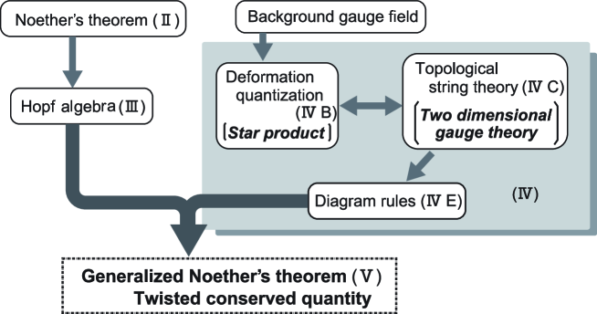
Figure 1: Flows of derivation of generalized Noether’s theorem. Roman numerals and capital letters in boxes represent section and subsection numbers, respectively. A generalization of the Noether’s theorem is achieved through Hopf algebra and deformation quantization (section V). Hopf algebra appear to characterize feature of an infinitesimal transformed variation operator (sections I​ I and I​ I​ I). The SU(2) gauge structure is embedded in the star product (section I​ V).

II Noether’s theorem in field theory

In this section, we discuss Noether’s theorem ConservationTheorems , and its generalization as a motivation to introduce the Hopf algebra and deformation quantization. In section II.1, we will recall Noether theorem, and rewrite it using the so-called “coproduct”, which is an element of the Hopf algebra. In section II.2, we will sketch a derivation of generalized Noether theorem.

II.1 Conventional formulation of Noether’s theorem

We start with the action $I$ given by

$$I = \int_{\Omega}d^{\rm Dim}x{\cal L}(x)$$ (7)

$$= \int d^{\rm Dim}xh_{\Omega}(x){\cal L}(x),$$

where $\Omega$ represents a range of the spacetime coordinate $x$ ($\equiv(x^{0},x^{i})\equiv(ct,\bm{x})$) with a dimension Dim, i.e., $({\rm Dim}-1)$ is the dimension of the space, ${\mathcal{L}}$ describes a Lagrangian density, and

$$h_{\Omega}(x)=\left\{\begin{array}[]{ccc}1&{\rm for}&\{x|x\in\Omega\}\\ 0&{\rm for}&\{x|x\notin\Omega\}.\end{array}\right.;$$ (8)

$c$ represents light speed. We introduce a field $\phi_{r}$ with internal degree of freedom $r$, and infinitesimal transformations:

$$x^{\mu}\mapsto({x^{\prime}})^{\mu}:=x^{\mu}+\delta_{\zeta}x^{\mu},$$ (9)

$$\phi_{r}(x)\mapsto\phi^{\prime}_{r}(x^{\prime}):=\phi_{r}(x)+\delta_{\zeta}\phi_{r}(x),$$ (10)

where we characterize the transformations by the subscript; specifically, $\zeta$ represents a general infinitesimal transformation. Hereafter, we will employ Einstein summation convention, i.e., $a^{\mu}b_{\mu}\equiv a_{\mu}b^{\mu}\equiv\sum_{\mu=0}^{{\rm Dim}-1}\eta_{\mu\nu}a^{\mu}b^{\mu}$ with vectors $a^{\mu}$ and $b^{\mu}$ $(\mu=0,1,\ldots,({\rm Dim}-1))$, and the Minkowski metric: $\eta_{\mu\nu}:={\rm diag}(-1,\underbrace{1,1,\ldots,1}_{{\rm Dim}-1})$.

We define the variation operator of the action as follow:

$$\delta_{\zeta}I := \int_{\Omega^{\prime}}{d^{\rm Dim}x^{\prime}}{\cal L}^{\prime}({x^{\prime}})-\int_{\Omega}d^{\rm Dim}x{\cal L}(x)$$ (11)

$$= \int{d^{\rm Dim}x^{\prime}}h_{\Omega^{\prime}}(x^{\prime}){\cal{L^{\prime}}}({x^{\prime}})-\int{d^{\rm Dim}x}h_{\Omega}(x){\cal L}(x),$$

where we characterize this variation by $\zeta$, because this variation is derived from the infinitesimal transformations Eqs. (9) and (10). Since the integration variable $x^{\prime}$ can be replaced by $x$, Eq. (11) is

$$\delta_{\zeta}I = \int{d^{\rm Dim}x}h_{\Omega^{\prime}}(x){\cal{L^{\prime}}}(x)-\int{d^{\rm Dim}x}h_{\Omega}(x){\cal L}(x)$$ (12)

$$= \int{d^{\rm Dim}x}\left(h_{\Omega^{\prime}}(x)-h_{\Omega}(x)\right){\cal{L^{\prime}}}(x)+\int{d^{\rm Dim}x}h_{\Omega}(x)\left[{\cal L}^{\prime}(x)-{\cal L}(x)\right]$$

$$= \int d^{\rm Dim}xh_{\delta\Omega}(x){\cal L}^{\prime}(x)+\int d^{\rm Dim}xh_{\Omega}(x)\left[{\cal L}^{\prime}(x)-{\cal L}(x)\right],$$

where $\delta\Omega:=\Omega^{\prime}-\Omega$ and $h_{\delta\Omega}=-(\partial_{\mu}h_{\Omega})\delta_{\zeta}x^{\mu}+{\cal O}((\delta_{\zeta}x)^{2})$. Therefore, we obtain the following equation through partial integration:

$$\delta_{\zeta}I = \int{d^{\rm Dim}x}h_{\Omega}(x)\left[\partial_{\mu}({\cal L}(x)\delta_{\zeta}x^{\mu})+\delta^{\rm L}_{\zeta}{\cal L}(x)\right]+{\cal O}((\delta_{\zeta}x)^{2}),$$ (13)

where we have introduced the so-called Lie derivative:

$$\delta^{\rm L}_{\zeta}\phi_{r}(x) := \phi^{\prime}_{r}(x)-\phi_{r}(x)$$ (14)

$$= \delta_{\zeta}\phi_{r}(x)-(\partial_{\mu}\phi_{r})\delta_{\zeta}x^{\mu}+{\cal O}(\delta_{\zeta}x^{2}),$$

and we replaced ${\cal L}^{\prime}$ by ${\cal L}$ due to ${\cal L}^{\prime}\delta_{\zeta}x^{\mu}={\cal L}\delta_{\zeta}x^{\mu}+{\cal O}(\delta_{\zeta}x^{2})$.

Hereafter, we assume that the action is invariant under the infinitesimal transformations Eqs. (9) and (10). In the case where the Lagrangian density is a function of $\phi_{r}$ and $\partial_{\mu}\phi_{r}$, i.e., ${\cal L}(x)={\cal L}\left[\phi_{r}(x),\partial_{\mu}\phi_{r}(x)\right]$, the Lie derivative of the Lagrangian is given by

$$\delta^{\rm L}_{\zeta}{\cal L} := {\cal L}^{\prime}(x)-{\cal L}(x)$$ (15)

$$= {\cal L}\left[\phi_{r}^{\prime}(x),\partial_{\mu}\phi_{r}^{\prime}(x)\right]-{\cal L}\left[\phi_{r}(x),\partial_{\mu}\phi_{r}(x)\right]$$

$$= \left\{\frac{\partial{\cal L}}{\partial\phi_{r}}\delta^{\rm L}_{\zeta}\phi_{r}+\frac{\partial{\cal L}}{\partial\left(\partial_{\mu}\phi_{r}\right)}\partial_{\mu}\delta^{\rm L}_{\zeta}\phi_{r}\right\}$$

$$= \left(\frac{\partial{\cal L}}{\partial\phi_{r}}-\partial_{\mu}\frac{\partial{\cal L}}{\partial(\partial_{\mu}\phi_{r})}\right)\delta^{\rm L}_{\zeta}\phi_{r}+\partial_{\mu}\left(\frac{\partial{\cal L}}{\partial(\partial_{\mu}\phi_{r})}\delta^{\rm L}_{\zeta}\phi_{r}\right),$$

and the variation of the action is calculated by

$$\delta_{\zeta}I=\int_{\Omega}d^{\rm Dim}x\left\{\left(\frac{\partial{\cal L}}{\partial\phi_{r}}-\partial_{\mu}\frac{\partial{\cal L}}{\partial(\partial_{\mu}\phi_{r})}\right)\delta^{\rm L}_{\zeta}\phi_{r}+\partial_{\mu}\left({\cal L}\delta_{\zeta}x^{\mu}+\frac{\partial{\cal L}}{\partial(\partial_{\mu}\phi_{r})}\delta^{\rm L}_{\zeta}\phi_{r}\right)\right\}.$$ (16)

If we require that $\delta_{\zeta}x$ and $\delta^{\rm L}_{\zeta}\phi_{r}$ vanish on the surface $\partial\Omega$, we obtain the Euler-Lagrange equation. On the other hand, if we require that fields $\phi_{r}$ satisfy the Euler-Lagrange equation, we obtain continuity equation $\partial_{\mu}j^{\mu}=0$ with a Noether current

$$j^{\mu}:=\left({\cal L}\delta_{\zeta}x^{\mu}+\frac{\partial{\cal L}}{\partial(\partial_{\mu}\phi_{r})}\delta^{\rm L}_{\zeta}\phi_{r}\right).$$ (17)

Hereafter let us discuss an infinitesimal global U(1)$\times$SU(2) gauge transformation and infinitesimal translation and rotation transformations, which are denoted by $\chi$ in this paper. Variations in terms of $\chi$ are defined by

$$\delta_{\chi}x^{\mu} := \Gamma^{\mu}_{\nu}x^{\nu},$$ (18)

$$\delta_{\chi}\phi_{r} := \mbox{i}\vartheta^{\mu\nu}(\xi_{\mu\nu})_{r}^{r^{\prime}}\phi_{r^{\prime}}$$ (19)

with an infinitesimal parameter $\vartheta^{\mu\nu}$, and symmetry generators $\Gamma^{\mu}_{\nu}$ and $(\xi_{\mu\nu})_{r}^{r^{\prime}}$.

1. For the global U(1)$\times$SU(2) gauge transformation, $\Gamma^{\mu}_{\nu}\equiv 0$, $\vartheta^{\mu\nu}\equiv\vartheta^{\mu}\delta^{\mu\nu}$, and $(\xi_{\mu\nu})_{r}^{r^{\prime}}\equiv\delta_{\mu\nu}(\hat{s}_{\mu})_{r}^{r^{\prime}}$ ($\mu,\nu=0,1,2,3$; $r,r^{\prime}=1,2$), where $\hat{s}^{0}:=\hbar/2$, and $\hat{s}^{1,2,3}:=\hbar\hat{\sigma}^{x,y,z}/2$ with the Planck constant $h=2\pi\hbar$ and Pauli matrices $\hat{\sigma}^{x,y,z}$.

2. For the translation, $\Gamma^{\mu}_{\nu}\equiv\varepsilon^{\mu}\delta^{\mu}_{\nu}$, $\vartheta^{\mu\nu}\equiv\varepsilon^{\mu}\delta^{\mu\nu}$ and $(\xi_{\mu\nu})_{r}^{r^{\prime}}\equiv\hat{p}_{\mu}\delta_{\mu\nu}\delta_{r}^{r^{\prime}}$ with an infinitesimal parameter $\varepsilon^{\mu}$ and the momentum operator $\hat{p}_{\mu}=-{\rm i}\hbar\partial_{\mu}$ ($\mu,\nu=1,2,3$; $r,r^{\prime}=1,2$).

3. For the rotation, $\Gamma^{\mu}_{\nu}\equiv\omega^{\mu}_{\nu}$, $\vartheta^{\mu\nu}\equiv\omega^{\mu\nu}$, and $(\xi_{\mu\nu})_{r}^{r^{\prime}}\equiv\delta_{r}^{r^{\prime}}x_{\mu}\hat{p}_{\nu}$, which corresponds to the angular momentum tensor ($\mu,\nu=1,2,3$; $r,r^{\prime}=1,2$).

For these transformations, equation $\partial_{\mu}\delta_{\chi}x^{\mu}=0$ is satisfied. This can be seen explicitly as follows. The variations of space coordinates of the global U(1)$\times$SU(2) and the translation transformations are given by $\delta_{\chi}x^{\mu}=0$ or $\delta_{\chi}x^{\mu}={\rm constant}$, respectively, and thus $\partial_{\mu}\delta_{\chi}x^{\mu}=0$ is trivial. The variation of the rotation transformation is given by $\delta_{\chi}x^{\mu}=\omega^{\mu}_{\nu}x^{\nu}$, therefore $\partial_{\mu}\delta_{\chi}x^{\mu}=\partial_{\mu}\omega^{\mu}_{\nu}x^{\nu}=\omega^{\mu}_{\mu}=0$.

We consider a variation of the Lagrangian density;

$$\delta_{\zeta}{\cal L} := {\cal L}^{\prime}(x^{\prime})-{\cal L}(x)$$ (20)

$$= {\cal L}^{\prime}(x^{\prime})-{\cal L}(x^{\prime})+{\cal L}(x^{\prime})-{\cal L}(x)$$

$$= \delta^{\rm L}_{\zeta}{\cal L}(x^{\prime})+\delta_{\zeta}x^{\mu}\partial_{\mu}{\cal L}+{\cal O}((\delta_{\zeta}x)^{2}).$$

Note that Eq. (20) is correct for any infinitesimal transformation. Here we consider the global U(1)$\times$SU(2) gauge transformation and/or the translation and rotation transformations $\delta_{\chi}$. Because $\partial_{\mu}\delta_{\chi}x^{\mu}=0$, we obtain the following equation:

$$\delta_{\chi}{\cal L}=\delta^{\rm L}_{\chi}{\cal L}(x)+\partial_{\mu}({\cal L}(x)\delta_{\chi}x^{\mu})+{\cal O}((\delta x)^{2}).$$ (21)

From Eqs.(13) and (21), one can see

$$\delta_{({\zeta=\chi})}I=\int d^{\rm Dim}x\delta_{\chi}{\cal L}(x),$$ (22)

where ${(\zeta=\chi)}$ denotes that the type of the variation in Eq. (13) is restricted to the global U(1)$\times$SU(2) or Poincare transformations. (For simplicity we omitted the subscript $\Omega$ in the integral). Finally, for $\zeta=\chi$, the variation of the action is equal to the variation of Lagrangian. This fact will be used later in section V where the variation of the Lagrangian density instead of the action will be considered.

II.2 Generalization of Noether’s theorem

Now, we would like to introduce a Hopf algebra for the purpose of generalizing Noether’s theorem  Gonera2005192 ; PTPS.171.65 ; AmelinoCamelia2009298 . At first, we rewrite Noether’s theorem in section II by using the Hopf algebra, and next, we introduce a twisted symmetry  Chaichian200498 ; PhysRevLett.94.151602 . For simplicity, we only consider the global U(1)$\times$SU(2) gauge symmetry and the Poincare symmetry. We assume that the Lagrangian density is written as

$${\cal L}(x)=\psi^{\dagger}(x)\hat{{\cal L}}(x)\psi(x)$$ (23)

with a field $\psi:=\left(\begin{array}[]{c}\psi_{1}\\ \psi_{2}\end{array}\right)$, a Hermitian conjugate $\psi^{\dagger}\equiv\left(\overline{\psi}_{1},\overline{\psi}_{2}\right)$, and an single-particle Lagrangian density operator $\hat{\cal L}$, which is a 2$\times$2 matrix; the overline represents the complex conjugate. The action can be rewritten as

$$I = \int d^{\rm Dim}x_{1}d^{\rm Dim}x_{2}\psi^{\dagger}(x_{2})\delta(x_{2}-x_{1})\hat{{\cal L}}(x_{1})\psi(x_{1})$$ (24)

$$= {\rm tr}\int d^{\rm Dim}x_{1}d^{\rm Dim}x_{2}\delta(x_{2}-x_{1})\hat{{\cal L}}(x_{1})\psi(x_{1})\psi^{\dagger}(x_{2})$$

$$= {\rm tr}\int d^{\rm Dim}x_{1}\left\{\int d^{\rm Dim}x_{2}{\tilde{\cal L}}(x_{1},x_{2})G(x_{2},x_{1})\right\}$$

$$= {\rm tr}\int d^{\rm Dim}x_{1}\left\{\lim_{x_{3}\rightarrow x_{1}}(\tilde{\cal L}*_{C}G)(x_{1},x_{3})\right\},$$

where “${\rm tr}$” represents the trace in the spin space, $G(x_{1},x_{2}):=\psi(x_{1})\psi^{\dagger}(x_{2})$, $\tilde{{\cal L}}(x_{1},x_{2}):=\delta(x_{1}-x_{2})\hat{{\cal L}}(x_{2})$, and $*_{C}$ represents the convolution integral:

$$(f*_{C}g):=\int d^{\rm Dim}x_{3}f(x_{1},x_{3})g(x_{3},x_{2})$$ (25)

with smooth two-variable functions $f$ and $g$.

The variation operator $\delta_{\chi}$ of the action can be also rewritten as

$$\delta_{\chi}I = {\rm tr}\int d^{\rm Dim}x_{1}d^{\rm Dim}x_{2}\tilde{\cal L}(x_{2},x_{1})\left[i\vartheta\xi\psi(x_{1})\psi^{\dagger}(x_{2})-\psi(x_{1})\psi^{\dagger}(x_{2})i\vartheta\xi\right]$$

$$= {\rm tr}\int d^{\rm Dim}x_{1}d^{\rm Dim}x_{2}\left[\tilde{{\cal L}}(x_{2},x_{1})i\vartheta\xi G(x_{1},x_{2})-i\vartheta\xi\tilde{{\cal L}}(x_{2},x_{1})G(x_{1},x_{2})\right]$$

with $\vartheta\xi\equiv\vartheta^{\mu\nu}(\xi_{\mu\nu})$; in addition, we assumed that the single-particle Lagrangian density operator is invariant under the infinitesimal transformation $\delta_{\chi}$.

Here, we introduce Grassmann numbers $\theta_{1}$ and $\theta_{2}$; an integral is defined by $\int d\theta_{i}\left(\theta_{j}\right)=\delta_{ij}$. The variation of the right-hand side of Eq.(LABEL:eq:VariationXi) can be rewritten as follow:

$$\delta_{\chi}I = -{\rm i}{\rm tr}\int d\theta_{1}d\theta_{2}d^{\rm Dim}x_{1}d^{\rm Dim}x_{2}\left[\theta_{1}\tilde{\cal L}(x_{2},x_{1})\vartheta\theta_{2}\xi G(x_{1},x_{2})+\vartheta\theta_{2}\xi\theta_{1}\tilde{\cal L}(x_{2},x_{1})G(x_{1},x_{2})\right]$$ (27)

$$= -{\rm i}{\rm tr}\int d\theta_{1}d\theta_{2}d^{\rm Dim}x_{1}d^{\rm Dim}x_{2}\mu\circ(\mu\otimes\mbox{id})$$

$$\circ\left[\left(\theta_{1}\tilde{\cal L}(x_{2},x_{1})\otimes\vartheta\theta_{2}\xi+\vartheta\theta_{2}\xi\otimes\theta_{1}\tilde{\cal L}(x_{2},x_{1})\right)\otimes G(x_{1},x_{2})\right]$$

$$= -{\rm i}{\rm tr}\int d\theta_{1}d\theta_{2}d^{\rm Dim}x_{1}d^{\rm Dim}x_{2}\mu\circ(\mu\otimes{\rm id})\left[\triangle(\vartheta\theta_{2}\xi)\circ\left(\theta_{1}\tilde{\cal L}(x_{2},x_{1})\otimes G(x_{1},x_{2})\right)\right]$$

$$\equiv {\rm\hat{T}r}\left[\triangle(\vartheta\theta_{2}\xi)\circ((\theta_{1}\tilde{\cal L})\otimes G)\right],$$

where $\otimes$ and $\circ$ represent a tensor product and a product of operators, respectively. The operator $\mu$ denotes the transformation of the tensor product to the usual product $\mu:x\otimes y\mapsto xy$, and $\triangle$ represents a coproduct:

$$\triangle(\zeta):=\zeta\otimes{\rm id}+{\rm id}\otimes\zeta,$$ (28)

where $\zeta$ and ${\rm id}$ represent a certain operator and the identity map, respectively. These operators constitutes the Hopf algebra as will be explained in the next section. Moreover, we have defined ${\rm\hat{T}r}:=-{\rm i}{\rm tr}\int d\theta_{1}d\theta_{2}d^{\rm Dim}x_{1}d^{\rm Dim}x_{2}\mu\circ(\mu\otimes{\rm id})$. We emphasize here that the variation is written by the coproduct $\triangle$, which is important to formulate the generalized Noether theorem in the presence of the gauge potential. The coproduct determines an operation rule of a variation operator; for example, the coproduct (28) represents the Leibniz rule. A twisted symmetry transformation is given by deformation of the coproduct.

We now sketch the concept of the twisted symmetry in deformation quantization Chaichian200498 ; PhysRevLett.94.151602 . First, we assume that the variation of action $\delta_{\zeta}I_{0}$ is zero, i.e., $\zeta$ represents the symmetry transformation of the system corresponding to the action $I_{0}$. Next, we consider the action $I_{A}$ with external gauge fields $A$. Usually, external gauge fields breaks symmetries of $I_{0}$, i.e., $\delta_{\zeta}I_{A}\neq 0$. Here we introduce a map: ${\cal F}_{(0\mapsto A)}:I_{0}\mapsto I_{A}$, which will be defined in section IV.6. The basic idea is to generalize the ”product” taking into account the gauge interaction. Using this map, the variation is rewritten as $\delta_{\zeta}{\cal F}_{(0\mapsto A)}I_{0}\neq 0$. On the other hand, when the twisted symmetry $\delta^{t}_{\zeta}:={\cal F}_{(0\mapsto A)}\delta_{\zeta}{\cal F}^{-1}_{(0\mapsto A)}$ can be defined, we obtain the following equation:

$$\delta^{t}_{\chi}I_{A} = {\cal F}_{(0\mapsto A)}\delta_{\chi}{\cal F}^{-1}_{(0\mapsto A)}I_{A}$$ (29)

$$= {\cal F}_{(0\mapsto A)}\delta_{\chi}{\cal F}^{-1}_{(0\mapsto A)}{\cal F}_{(0\mapsto A)}I_{0}$$

$$= {\cal F}_{(0\mapsto A)}\delta_{\chi}I_{0}$$

$$= 0.$$

Namely, $\delta^{t}_{\chi}$ corresponds to a symmetry with external gauge fields. In the expression for the variation of action in terms of the Hopf algebra Eq.(27), we can replace $\Delta$ by $\Delta^{t}$ corresponding to the change from $\delta\chi$ to $\delta^{t}_{\chi}$ as shown in section V. This is achieved by using the Hopf algebra and the deformation quantization, which will be explained in sections III and IV, respectively. Therefore, we can generalize the Noether’s theorem and derive the conservation law even in the presence of the gauge field $A$.

III Hopf algebra

Here we introduce a Hopf algebra. First, we rewrite the algebra using tensor and linear maps. Secondly, a coalgebra is defined using diagrams corresponding to the algebra. Finally, we define a dual-algebra and Hopf algebra.

III.0.1 Algebra

We define the algebra as a $k$-vector space $V$ having product $\mu$ and unit $\varepsilon$. Here, $k$ represents a field such as the complex number or real number. In this paper, we consider $V$ as the space of functions or operators. A space of linear maps from a vector space $V_{1}$ to a vector space $V_{2}$ is written as ${\rm Hom}(V_{1},V_{2})$.

A product $\mu$ is a bilinear map: $\mu\in{\rm Hom}(V\bigotimes V,V)$, i.e.,

$$\mu:V\bigotimes V\rightarrow V,\ \ \ \ \ (x,y)\mapsto xy,$$ (30)

and a unit is a linear map: $\varepsilon\in{\rm Hom}(k,V)$, i.e.,

$$\varepsilon:k\rightarrow V,\ \ \ \ \ \alpha\mapsto\alpha\cdot 1$$ (31)

with $x,y,xy\in V$ and $\alpha\in k$. Here $\mu$ and $\varepsilon$ satisfies

$$\mu((x+y)\otimes z)=\mu(x\otimes z)+\mu(y\otimes z),~{}\mu(x\otimes(y+z))=\mu(x\otimes y)+\mu(x\otimes z),$$ (32)

$$\mu(\alpha x\otimes y)=\alpha\mu(x\otimes y),~{}\mu(x\otimes\alpha y)=\alpha\mu(x\otimes y),$$ (33)

$$\varepsilon(\alpha+\beta)=\varepsilon(\alpha)+\varepsilon(\beta)$$ (34)

with $x,y,z\in V$ and $\alpha,\beta\in k$.

The product $\mu$ has the association property, which is written as $\mu\circ({\rm id}\otimes\mu)=\mu\circ(\mu\otimes{\rm id})$. Because the left-hand side and the right-hand side of the previous equation give the following equations:

$$\mu\circ({\rm id}\otimes\mu)(x\otimes y\otimes z)=\mu(x\otimes(yz))=x(yz)$$ (35)

and

$$\mu\circ(\mu\otimes{\rm id})(x\otimes y\otimes z)=\mu((xy\otimes z))=(xy)z,$$ (36)

for all $x,y,z,xy,yz,xyz\in V$, then $\mu\circ({\rm id}\otimes\mu)=\mu\circ(\mu\otimes{\rm id})$ is equal to the association property $x(yz)=(xy)z$. This property is illustrated as the following diagram:

Here $\circlearrowright$ denotes that this graph is the commutative diagram.

The unit $\varepsilon$ satisfies the following equation: $\mu\circ(\varepsilon\otimes{\rm id})=\mu\circ({\rm id}\otimes\varepsilon)$. Since the left-hand side and the right-hand side of the previous equation give the following equations

$$\mu\circ(\varepsilon\otimes{\rm id})(\alpha\otimes x)=\mu\otimes(\alpha 1_{V}\otimes x)=\alpha 1_{V}x=\alpha x$$ (37)

and

$$\mu\circ({\rm id}\otimes\varepsilon)(x\otimes\alpha)=\mu\circ(x\otimes\alpha 1_{V})=\alpha x1_{V}=\alpha x$$ (38)

for all $x\in V$ and $\alpha\in k$, and ${}^{\exists}1_{V}\in V$, then the unit can be written as $\mu\circ({\rm id}\otimes\varepsilon)=\mu\circ(\varepsilon\otimes{\rm id})$. Note that $V\sim k\bigotimes V\sim V\bigotimes k$, where $\sim$ represents the equivalence relation, i.e., $a\sim b$ denotes that $a$ and $b$ are identified. This property is illustrated as:

Algebra is defined as a set $(V,\mu,\varepsilon)$.

III.0.2 Coalgebra

A coalgebra is defined by reversing the direction of the arrows in the diagrams corresponding to the algebra. Thus, we will define a coproduct $\triangle\in{\rm Hom}(V,V\bigotimes V)$ and counit $\eta\in{\rm Hom}(V,V)$ with a $k$-vector space $V$.

A coproduct is a bilinear map from $V$ to $V\bigotimes V$:

$$\triangle:V\rightarrow V\bigotimes V,$$ (39)

and satisfies co-association property:

Namely,

$$({\rm id}\otimes\triangle)\circ\triangle=(\triangle\otimes{\rm id})\circ\triangle$$ (40)

(Compare the diagram corresponding to the association property and that corresponding to the co-association property).

A counit $\eta$ is a linear map from $V$ to field $k$:

$$\eta:V\rightarrow k,$$ (41)

and satisfies the following diagram:

Namely,

$$(\eta\otimes{\rm id})\circ\triangle=({\rm id}\otimes\eta)\circ\triangle,$$ (42)

where $V\sim k\bigotimes V\sim V\bigotimes k$.

Since $\triangle$ and $\eta$ are linear maps, $\triangle$ and $\eta$ satisfy

$$\triangle(x+y)=\triangle(x)+\triangle(y),~{}\triangle(\alpha x)=\alpha\triangle(x),$$ (43)

$$\eta(x+y)=\eta(x)+\eta(y),~{}\eta(\alpha x)=\alpha\eta(x)$$ (44)

with $x,y\in V$ and $\alpha\in k$. Note that $V\sim k\bigotimes V\sim V\bigotimes k$ and $V\bigotimes V\sim k\bigotimes V\bigotimes V\sim V\bigotimes k\bigotimes V\sim V\bigotimes V\bigotimes k$.

A coalgebra is defined as a set $(V,\triangle,\eta)$. For example, in the vector space $D\equiv k\bigoplus k\partial:=\{a_{0}+a_{1}\partial|a_{0},a_{1}\in k\}$, we define a coproduct $\triangle_{D}(\partial)=\partial\otimes 1+1\otimes\partial$ and $\triangle_{D}(1)=1\otimes 1$, and a counit $\eta_{D}(\partial)=0$ and $\eta_{D}(1)=1$. The set $(D,\triangle_{D},\eta_{D})$ is coalgebra, because this set satisfies the equations: $(\triangle_{D}\otimes{\rm id})\circ\triangle_{D}=({\rm id}\otimes\triangle_{D})\circ\triangle_{D}$ and $(\eta_{D}\otimes{\rm id})\circ\triangle_{D}=({\rm id}\otimes\eta_{D})\circ\triangle_{D}$. Because the coproduct and counit are linear map, we only check the above equations with respect to $x=1$ and $\partial$.

For $x=1$,

$$(\triangle_{D}\otimes{\rm id})\circ\triangle_{D}(1)=\triangle_{D}(1)\otimes 1=1\otimes 1\otimes 1,$$ (45)

and

$$({\rm id}\otimes\triangle_{D})\circ\triangle_{D}(1)=1\otimes\triangle_{D}(1)=1\otimes 1\otimes 1.$$ (46)

Therefore, $(\triangle_{D}\otimes{\rm id})\circ\triangle_{D}(1)=({\rm id}\otimes\triangle_{D})\circ\triangle_{D}(1)$. Moreover,

$$(\eta_{D}\otimes{\rm id})\circ\triangle_{D}(1)=\eta_{D}(1)\otimes 1=1\otimes 1,$$ (47)

and

$$({\rm id}\otimes\eta_{D})\circ\triangle_{D}(1)=1\otimes\eta_{D}(1)=1\otimes 1.$$ (48)

Therefore $(\eta_{D}\otimes{\rm id})\circ\triangle_{D}(1)=({\rm id}\otimes\eta_{D})\circ\triangle_{D}(1)$.

For $x=\partial$,

$$(\triangle_{D}\otimes{\rm id})\circ\triangle_{D}(\partial)=\triangle_{D}(\partial)\otimes 1+\triangle_{D}(1)\otimes\partial=\partial\otimes 1\otimes 1+1\otimes\partial\otimes 1+1\otimes 1\otimes\partial,$$ (49)

and

$$({\rm id}\otimes\triangle_{D})\circ\triangle_{D}(\partial)=\partial\otimes\triangle_{D}(1)+1\otimes\triangle_{D}(\partial)=\partial\otimes 1\otimes 1+1\otimes\partial\otimes 1+1\otimes 1\otimes\partial.$$ (50)

Therefore, $({\rm id}\otimes\triangle_{D})\circ\triangle_{D}(\partial)=(\triangle_{D}\otimes{\rm id})\circ\triangle_{D}(\partial)$. Finally,

$$(\eta_{D}\otimes{\rm id})\circ\triangle_{D}(\partial)=\eta_{D}(\partial)\otimes 1+\eta_{D}(1)\otimes\partial=1\otimes\partial=\partial,$$ (51)

and

$$({\rm id}\otimes\eta_{D})\circ\triangle_{D}(\partial)=\partial\otimes\eta_{D}(1)+1\otimes\eta_{D}(\partial)=\partial\otimes 1=\partial.$$ (52)

Therefore, $(\eta_{D}\otimes{\rm id})\circ\triangle_{D}(\partial)=({\rm id}\otimes\eta_{D})\circ\triangle_{D}(\partial)$. Namely, the set $(D,\triangle_{D},\eta_{D})$ is the coalgebra. Note that $\triangle_{D}(1)$ corresponds to the product with a constant: $a(fg)=a1(fg)=a(1f1g)=a\mu\circ\triangle_{D}(1)(f\otimes g)$, where we have used the coproduct $\triangle_{D}(1)=1\otimes 1$ at the final equal sign. Here $f,~{}{\rm and}~{}g$ are smooth functions, $1$ is included in the function space, and $a\in k$. $\triangle_{D}(\partial)$ represents the Leibniz rule: $\partial(fg)=(\partial f)g+f\partial(g)=\mu\circ(\partial\otimes 1+1\otimes\partial)\circ(f\otimes g)=\mu\circ\triangle_{D}(\partial)(f\otimes g)$, where we have used the coproduct $\triangle_{D}(\partial)=1\otimes\partial+\partial\otimes 1$ at the last equal sign. $\eta_{D}(1)$ and $\eta_{D}(\partial)$ represent the filtering action to a constant function: $1a=a=\eta_{D}(1)a$ and $\partial(a)=0=\eta_{D}(\partial)a$, respectively.

III.0.3 Dual-algebra and Hopf algebra

A dual-algebra is the set of an algebra and a coalgebra, i.e., the set of $(V,\mu,\varepsilon,\triangle,\eta)$. On a dual-algebra, we define a $*$-product as

$$f*g=\mu\circ(f\otimes g)\circ\triangle$$ (53)

with $f,g\in{\rm Hom}(V,V)$. We define an antipode $S\in{\rm Hom}(V,V)$ which satisfies the following equation:

$$\mu\circ({\rm id}\otimes S)\circ\triangle=\mu\circ(S\otimes{\rm id})\circ\triangle=\varepsilon\circ\eta,$$ (54)

where $\varepsilon\circ\eta$ corresponds to the identity mapping, i.e., $S$ is an inverse of unit. For example, $S_{D}$ in the set $(D,\mu_{D},\varepsilon_{D},\triangle_{D},\eta_{D})$ is defined as $S_{D}(1)=1$ and $S_{D}(\partial)=-\partial$.

For $x=1$,

$$\mu_{D}\circ({\rm id}\otimes S_{D})\circ\triangle_{D}(1)=\mu_{D}\circ(1\otimes 1)=1,$$ (55)

and

$$\mu_{D}\circ(S_{D}\otimes{\rm id})\circ\triangle_{D}(1)=\mu_{D}\circ(1\otimes 1)=1.$$ (56)

Therefore, we obtain $\mu_{D}\circ({\rm id}\otimes S_{D})\circ\triangle_{D}(1)=\mu_{D}\circ(S_{D}\otimes{\rm id})\circ\triangle_{D}(1)=\varepsilon_{D}\circ\eta_{D}$. For $\partial$,

$$\mu_{D}\circ({\rm id}\otimes S_{D})\circ\triangle_{D}(\partial)=\mu_{D}\circ(\partial\otimes 1-1\otimes\partial)=0,$$ (57)

and

$$\mu_{D}\circ(S_{D}\otimes{\rm id})\circ\triangle_{D}(\partial)=\mu_{D}\circ(-\partial\otimes 1+1\otimes\partial)=0.$$ (58)

Therefore, we obtain $\mu_{D}\circ({\rm id}\otimes S_{D})\circ\triangle_{D}(\partial)=\mu_{D}\circ(S_{D}\otimes{\rm id})\circ\triangle_{D}(\partial)=\varepsilon_{D}\circ\eta_{D}(\partial)$. Namely, $(D,\mu_{D},\varepsilon_{D},\triangle_{D},\eta_{D})$ is the Hopf algebra.

A dual-algebra with an antipode $S$, i.e., $(V,\mu,\varepsilon,\triangle,\eta,S)$, is called a Hopf algebra.

By using the approach similar to a coproduct and counit, we can define a codifferential operator $Q\in{\rm Hom(V,V)}$ from a diagram of the differential $\partial\in{\rm Hom}(V,V)$. The differential $\partial$ is the linear map:

$$\partial:V\rightarrow V,$$ (59)

and satisfies Leibniz rule

$$\partial\circ\mu=\mu\circ({\rm id}\otimes\partial+\partial\otimes{\rm id}),$$ (60)

which is illustrated as

A codifferential operator $Q$ is a linear map; $Q:V\rightarrow V$, and satisfies the following diagrams:

Namely, a codifferential operator $Q$ satisfies $\triangle\circ Q=({\rm id}\otimes Q+Q\otimes{\rm id})\circ\triangle$. In section IV.2.2, the codifferential operator will be introduced.

IV Deformation quantization

In this section, we explain the deformation quantization using the noncommutative product encoding the commutation relationships. At first, in section IV.1, we introduce the so-called Wigner representation and Wigner space, and show that a product in the Wigner space is noncommutative. This product is called Moyal product and it guarantees the commutation relationship of the coordinate and canonical momentum. Next, we add spin functions and background gauge fields to the Wigner space, and rewrite the coordinates of Wigner space as a set of spacetime coordinates $X$, mechanical momenta $p$, and spins $s:=(s^{x},s^{y},s^{z})$ ($p$ includes the background gauge fields). To generalize the Moyal product for the deformed Wigner space, which is a set of function defined on $(X,p,s)$, we explain the general constructing method of the noncommutative product in section IV.2; the noncommutative product is the generalized Moyal product, which is called “star product”. This constructing method is given as a map from a Poisson bracket in the Wigner space to the noncommutative product (see section IV.2), and we see the condition of this deformation quantization map in section IV.2. This map is described by the path integral of a two-dimensional field theory, which is called the topological string theory. In section IV.3, we explain this topological string theory, and in section IV.4, we discuss the perturbative treatment of this theory. In section IV.5, we summarize the diagram technique. Finally, in section IV.6, we construct the star product in $(X,p,s)$ space. We note that the star product guarantees the background gauge structure.

IV.1 Wigner representation

We start with the introduction of the Wigner representation. From Equation (24), a natural product is the convolution integral:

$$(f*_{C}g)(x_{1},x_{2}):=\int d^{\rm Dim}x_{3}f(x_{1},x_{3})g(x_{3},x_{2}),$$ (61)

where $f,g\in{\cal G}$ with a two spacetime arguments function space ${\cal G}$. Here we introduce the center of mass coordinate $X$ and the relative coordinate $\xi$ as follows:

$$X\equiv(T,\bm{X}) := ((t_{1}+t_{2})/2,(\bm{x}_{1}+\bm{x}_{2})/2),$$ (62)

$$\xi\equiv(\xi_{t},\bm{\xi}) := (t_{1}-t_{2},\bm{x}_{1}-\bm{x}_{2}).$$ (63)

Moreover we employ the following Fourier transformation:

$${\cal F}_{\cal T}:f(x_{1},x_{2})\mapsto f(X,p)=\int d^{\rm Dim}\xi e^{-ip_{\mu}\xi^{\mu}/\hbar}f(X+\xi/2,X-\xi/2).$$ (64)

Now we define the Wigner space: ${\cal W}:=\{{\cal F}_{\cal T}[f]~{}|~{}f\in{\cal G}\}$ Wigner . In this space, the convolution is transformed to the so-called Moyal product Moyal ; SOnoda :

$$(f\star_{\cal M}g)(X,p):=f(X,p)e^{\frac{{\rm i}\hbar}{2}\left({\overleftarrow{\partial}}_{X}{\overrightarrow{\partial}}_{p_{\nu}}-{\overleftarrow{\partial}}_{p}{\overrightarrow{\partial}}_{X}\right)}g(X,p),$$ (65)

because

$${\cal F}_{\cal T}^{-1}[f\star_{\cal M}g] = \int\frac{d^{\rm Dim}p}{(2\pi\hbar)^{\rm Dim}}e^{ip_{\nu}\xi^{\nu}/\hbar}\left\{f(X,p)e^{\frac{{\rm i}\hbar}{2}\left({\overleftarrow{\partial}}_{X^{\nu}}{\overrightarrow{\partial}}_{p_{\nu}}-{\overleftarrow{\partial}}_{p_{\nu}}{\overrightarrow{\partial}}_{X^{\nu}}\right)}g(X,p)\right\}$$ (66)

$$= \int\frac{d^{\rm Dim}p}{(2\pi\hbar)^{\rm Dim}}d^{\rm Dim}\xi_{1}d^{\rm Dim}\xi_{2}e^{ip_{\nu}\xi^{\nu}/\hbar}\Big{\{}e^{-ip_{\nu}\xi_{1}/\hbar}f(X+\xi_{1}/2,X-\xi_{1}/2)$$

$$\times e^{\frac{{\rm i}\hbar}{2}\left({\overleftarrow{\partial}}_{X^{\nu}}{\overrightarrow{\partial}}_{p_{\nu}}-{\overleftarrow{\partial}}_{p_{\nu}}{\overrightarrow{\partial}}_{X^{\nu}}\right)}e^{-ip_{\nu}\xi^{\nu}_{2}/\hbar}g(X+\xi_{2}/2,X-\xi_{2}/2)\Big{\}}$$

$$= \int\frac{d^{\rm Dim}p}{(2\pi\hbar)^{\rm Dim}}d^{\rm Dim}\xi_{1}d^{\rm Dim}\xi_{2}e^{ip_{\nu}\left(\xi^{\nu}-\xi^{\nu}_{1}-\xi^{\nu}_{2}\right)/\hbar}$$

$$\times f(X+\xi_{1}/2,X-\xi_{1}/2)e^{\frac{1}{2}\left({\overleftarrow{\partial}}_{X^{\nu}}\xi^{\nu}_{2}-\xi^{\nu}_{1}{\overrightarrow{\partial}}_{X^{\nu}}\right)}g(X+\xi_{2}/2,X-\xi_{2}/2)$$

$$= \int d^{\rm Dim}\xi_{1}d^{\rm Dim}\xi_{2}\delta(\xi-\xi_{1}-\xi_{2})$$

$$\times f\left(X+\frac{\xi_{1}+\xi_{2}}{2},X-\frac{\xi_{1}-\xi_{2}}{2}\right)g\left(X-\frac{\xi_{1}-\xi_{2}}{2},X-\frac{\xi_{1}+\xi_{2}}{2}\right)$$

$$= \int d^{\rm Dim}x_{+}d^{\rm Dim}x_{-}\delta(\xi-x_{+})f\left(X+\frac{x_{+}}{2},x_{-}\right)g\left(x_{-},X-\frac{x_{+}}{2}\right)$$

$$= \int d^{\rm Dim}x_{-}f(X+\xi/2,x_{-})g(x_{-},X-\xi/2)$$

$$= f*_{C}g$$

with $\xi_{1}+\xi_{2}\equiv x_{+}$ and $\xi_{1}-\xi_{2}\equiv 2(X-x_{-})$.

In the Wigner space, the position operator $\hat{x}^{\mu}=x^{\mu}$ and the momentum operator $\hat{p}_{\mu}=-{\rm i}\hbar\partial_{\mu}$ becomes $X^{\mu}\star_{\cal M}$ and $p_{\mu}\star_{\cal M}$ because

$${\cal F}_{\cal T}[\hat{x}^{\mu}_{1}g(x_{1},x_{2})]=\int d^{\rm Dim}\xi e^{-\frac{{\rm i}}{\hbar}p_{\nu}\xi^{\nu}}\left(X^{\mu}+\xi^{\mu}/2\right)g(X+\xi/2,X-\xi/2)=\left(X^{\mu}+\frac{{\rm i}\hbar}{2}\partial_{p_{\mu}}\right)g(X,p)=X^{\mu}\star_{\cal M}g(X,p),$$ (67)

$${\cal F}_{\cal T}[\hat{x}^{\mu}_{2}g(x_{1},x_{2})]=\int d^{\rm Dim}\xi e^{-\frac{{\rm i}}{\hbar}p_{\nu}\xi^{\nu}}g(X+\xi/2,X-\xi/2)\left(X^{\mu}-\xi^{\mu}/2\right)=g(X,p)\star_{\cal M}X^{\mu},$$ (68)

$${\cal F}_{\cal T}[(\hat{p}_{1})_{\mu}g(x_{1},x_{2})]=\int d^{\rm Dim}\xi e^{-\frac{{\rm i}}{\hbar}p_{\nu}\xi^{\nu}}\frac{\hbar}{{\rm i}}\partial_{x_{1}^{\mu}}g(x_{1},x_{2})=p_{\mu}\star g(X,p),$$ (69)

and

$${\cal F}_{\cal T}[(\hat{p}_{2})_{\mu}g(x_{1},x_{2})]=\int d^{\rm Dim}\xi e^{-\frac{i}{\hbar}p_{\nu}\xi^{\nu}}\frac{\hbar}{{\rm i}}\partial_{x_{2}^{\mu}}g(x_{1},x_{2})=g(X,p)\star p_{\mu}.$$ (70)

The commutation relationship of operators is $[X^{\mu},p_{\nu}]_{\star_{\cal M}}:=X^{\mu}\star_{\cal M}p_{\nu}-p_{\nu}\star_{\cal M}X^{\mu}={\rm i}\hbar\delta^{\mu}_{\nu}$, which corresponds to the canonical commutation relationship of operators: $[\hat{x}^{\mu},\hat{p}_{\nu}]={\rm i}\hbar\delta^{\mu}_{\nu}$.

To add the spin arguments in ${\cal W}$, we will employ the following bilinear map:

$${\cal F}_{\cal M}\mapsto{\cal F}_{A=0}:=e^{\frac{{\rm i}\hbar}{2}\left(\partial_{X^{\mu}}\otimes\partial_{p_{\mu}}-\partial_{p_{\mu}}\otimes\partial_{X^{\mu}}\right)+\frac{i}{2}\epsilon^{abc}s^{a}\partial_{s^{b}}\otimes\partial_{s^{c}}}$$ (71)

with $\partial_{s^{a}}f:=f_{a}$ and $f\equiv f_{0}+\sum_{a=x,y,z}s^{a}f_{a}$. Note that the spin operator $\bm{\hat{s}}:=(\hat{s}^{x},\hat{s}^{y},\hat{s}^{z})$ is characterized by the commutation relation $[\hat{s}^{a},\hat{s}^{b}]={\rm i}\epsilon^{abc}\hat{s}^{c}$ $(a,b,c=x,y,z)$ with the Levi-Civita tensor $\epsilon^{abc}$, and the star product (71) reproduces the relation, i.e., the operator $(s^{a}\star)$ satisfies $[s^{a},s^{b}]_{\star}={\rm i}\epsilon^{abc}s^{c}$.

To obtain the map ${\cal F}_{(0\mapsto A)}:I_{0}\mapsto I_{A}$, we introduce the variables transformation $(X^{\mu},p_{\mu},\bm{s})\mapsto(X^{\mu},\hat{p}_{\mu},\bm{s})$ where

$$\hat{p}_{\mu}=p_{\mu}-qA^{a}_{\mu}(X^{\nu})s^{a}+eA_{\mu}$$ (72)

with $q=|e|/{\rm m}c^{2}$, the electric charge $-e=-|e|$, a U(1) gauge field $A_{\mu}$, and a SU(2) gauge field $A^{a}_{\mu}$. Their fields are treated as real numbers, and the integral over $p_{\mu}$ can be replaced by an integral over $\hat{p}_{\mu}$. This transformation induces the following transformations of differential operators:

$$\partial_{X^{\mu}}\otimes\partial_{p_{\mu}}-\partial_{p_{\mu}}\otimes\partial_{X^{\mu}}\mapsto\partial_{X^{\mu}}\otimes\partial_{\hat{p}_{\mu}}-\partial_{\hat{p}_{\mu}}\otimes\partial_{X^{\mu}}+q\left(\partial_{X^{\mu}}\hat{A}_{\nu}-\partial_{X^{\nu}}\hat{A}_{\mu}\right)\partial_{\hat{p}_{\mu}}\otimes\partial_{\hat{p}_{\nu}},$$ (73)

$$\epsilon^{abc}s^{a}\partial_{s^{b}}\otimes\partial_{s^{c}} \mapsto \epsilon^{abc}s^{a}\partial_{s^{b}}\otimes\partial_{s^{c}}-q\epsilon^{abc}A^{b}_{\mu}s^{a}\partial_{\hat{p}_{\mu}}\otimes\partial_{s^{c}}-q\epsilon^{abc}A^{c}_{\mu}s^{a}\partial_{s^{b}}\otimes\partial_{\hat{p}_{\mu}}$$ (74)

$$+q^{2}\epsilon^{abc}s^{a}A^{b}_{\mu}A^{c}_{\nu}\partial_{\hat{p}_{\mu}}\otimes\partial_{\hat{p}_{\nu}},$$

where $\hat{A}_{\mu}:=A_{\mu}^{a}s^{a}-(e/q)A_{\mu}$.

We expand ${\cal F}_{A=0}$ in terms of $\hbar$ as

$${\cal F}_{A=0}=\sum_{n=0}^{\infty}\left(\frac{{\rm i}\hbar}{2}\right)^{n}{\cal F}_{A=0}^{n}.$$ (75)

We define the bilinear map ${\cal F}_{A}$ corresponding to the commutation relation in terms of the phase space $(X^{\mu},\hat{p}_{\mu},\bm{s})$, and expand it in terms of $\hbar$ as

$${\cal F}_{A}=\sum_{n=0}^{\infty}\left(\frac{{\rm i}\hbar}{2}\right)^{n}{\cal F}_{A}^{n}.$$ (76)

From Eqs. (73) and (74), ${\cal F}_{A}^{1}$ is given as follows:

$${\cal F}_{A}^{1} = \partial_{X^{\mu}}\otimes\partial_{\hat{p}_{\mu}}-\partial_{\hat{p}_{\mu}}\otimes\partial_{X^{\mu}}+q\hat{F}_{\mu\nu}\partial_{\hat{p}_{\mu}}\otimes\partial_{\hat{p}_{\nu}}+\epsilon^{abc}s^{a}\partial_{s^{b}}\otimes\partial_{s^{c}}$$ (77)

$$-q\epsilon^{abc}s^{a}A^{b}_{\mu}\partial_{\hat{p}_{\mu}}\otimes\partial_{s^{c}}+q\epsilon^{abc}s^{a}A^{b}_{\mu}\partial_{s^{c}}\otimes\partial_{\hat{p}_{\mu}}$$

with $\hat{F}_{\mu\nu}:=\partial_{X^{\mu}}\hat{A}_{\nu}-\partial_{X^{\nu}}\hat{A}_{\mu}+(q/\hbar)\varepsilon^{abc}s^{a}\hat{A}^{b}_{\mu}\hat{A}^{b}_{\nu}$. Note that $\mu\circ{\cal F}_{A}^{1}$ is the Poisson bracket.

A constitution method of higher order terms ${\cal F}^{n}_{A}$ with $n>1$ is called a deformation quantization, which is given by Kontsevich Kontsevich , as will be described in the next subsection.

IV.2 Star product

In this subsection, we explain the Kontsevich’s deformation quantization method Kontsevich . We define a star product as

$$f\star g\equiv\mu\circ{\cal F}_{A}(f\otimes g)=f\cdot g+\sum_{n=1}^{\infty}\nu^{n}\beta_{n}(f\otimes g)$$ (78)

with $\nu={\rm i}\hbar/2$ Bayen197861 ; Bayen1978111 . Here $\beta_{n}\in{\rm Hom}\left(V_{f}\otimes V_{f},V_{f}\right)$ is called the two-cochain ($V_{f}$ represents the function space). We require that the star product satisfies the association property $(f\star g)\star h=f\star(g\star h)$, which limits forms of ${\cal F}^{n\geq 1}_{A}$ and $\beta_{n\geq 1}$. We note that the association property is necessary for the existence of the inverse with respect to the star product. For example, the inverse of the Lagrangian is a Green function, which always exists as $\psi\psi^{\dagger}$ with a wave function $\psi$.

Now, we define a $p$-cochain space ${\cal C}^{p}:={\rm Hom}(V_{f}^{\otimes p},V_{f})$ with $V^{\otimes p}_{f}\equiv\underbrace{V_{f}\otimes V_{f}\otimes\cdots\otimes V_{f}}_{p}$, where $V_{f}$ represents a function space such as the Wigner space ${\cal W}$; we define a multi-vector space ${\cal T}^{k}:=\Gamma({\cal M},\bigwedge^{k}TM)$, where ${\cal M}$ represents a manifold such as a classical phase space (dimension $d$), $TM:=\bigcup_{p\in{\cal M}}T_{p}M$ denotes a tangent vector bundle with a tangent vector space $T_{p}M\equiv\{\sum_{i}^{d}a^{i}(x)\partial_{x^{i}}\}$ at $p\in{\cal M}$ ($x$ is a coordinate at $p$; $a_{i}$ represents a certain coefficient), $\bigwedge^{k}$ denotes a $k$-th completely antisymmetric tensor product, (for example, $\partial_{i}\wedge\partial_{j}=\frac{1}{2!}(\partial_{i}\otimes\partial_{j}-\partial_{j}\otimes\partial_{i})\in\bigwedge^{2}TM$), and $\Gamma$ represents the section; for example, $\Gamma({\cal M},TM)$ is defined as a set of tangent vector at each position $p\in{\cal M}$. The Poisson bracket $\{f,g\}\equiv\alpha(f\otimes g):=\alpha^{ij}(x)(\partial_{i}\wedge\partial_{j})(f\otimes g)$ is element of ${\cal T}^{1}$, where $\alpha^{ij}=-\alpha^{ji}$ is called the Poisson structure $(i,j=1,2,\cdots,d)$.

The deformation quantization is the constitution method of higher order cochains $\beta_{n\geq 2}\in{\cal C}^{2}$ from the Poisson bracket $\alpha\in{\cal T}^{2}$. In other words, the deformation quantization is the following map ${\cal F}$:

$${\cal F}:~{} {\cal T}^{2}\rightarrow{\cal C}^{2}$$ (79)

$$\alpha\mapsto\beta\equiv\sum_{n\geq 1}\nu^{n}\beta_{n},$$

where $\alpha$ satisfies the Jacobi identity and $\beta$ satisfies the association property, as shown in Fig. 2(a).

In the following sections, we will generalize the two-cochain ${\cal C}^{2}$ and the second order differential operator ${\cal T}^{2}$ to the so-called $L_{\infty}$ algebra (the definition is given in section IV.2.2). In the section IV.2.1, we will introduce the two-cochain ${\cal C}^{2}$ and second order differential operator ${\cal T}^{2}$, and the $p$-cochain ${\cal C}^{p}$ and $k$-th order differential operator ${\cal T}^{k}$. We will show that these operators satisfy certain conditions, and ${\cal C}^{p}$ and ${\cal T}^{k}$ are embedded in a differential graded Lie algebra (d.g.L.a) (the definition is shown in section IV.2.1). Moreover, in section IV.2.2, the d.g.L.a will be embedded in the $L_{\infty}$ algebra (see Fig. 2(b)). In the $L_{\infty}$ algebra, the Jacobi identity and the association property are compiled in the following equation

$$Q(e^{\gamma})=0,$$ (80)

where $\gamma=\alpha~{}{\rm or}~{}\beta$, and $Q$ is called the codifferential operator, which will be introduced in section IV.2.2. Namely, in the $L_{\infty}$ algebra, the deformation quantization is a map from $\alpha\in{\cal T}^{2}$ to $\beta\in{\cal C}^{2}$ holding the solution of Eq. (80) (Figure 2(c)). Such a map is uniquely determined in the $L_{\infty}$ algebra.

In this paper, we will identify the tensor product $\otimes$ with the direct product $\times$, i.e., $V_{1}\bigotimes V_{2}\sim V_{1}\times V_{2}$: $f\otimes g\sim(f,g)$ with $f\in V_{1}$ and $g\in V_{2}$ ($a\sim b$ denotes that $a$ and $b$ are identified; $(f,g)$ represents the ordered pair, i.e., it is a set of $f$ and $g$, and $(a,b)\neq(b,a)$).

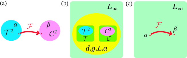
Figure 2: Steps of the derivation of the deformation quantization. (a): The image of the deformation quantization, which is the map from ${\cal T}^{2}$ with the Jacobi identity to ${\cal C}^{2}$ with the association property. (b): Enlargement of algebras. The two vector space ${\cal T}^{2}$ and two cochain space ${\cal C}^{2}$ generalize to multi-vector space ${\cal T}$ and cochain space ${\cal C}$, respectively. These spaces are compiled in the d.g.L.a; finally, $L_{\infty}$ algebra is introduced by using the d.g.L.a. (c): The deformation quantization is redefined as the map on the $L_{\infty}$ algebra.

IV.2.1 Cohomology equation

From Eq. (78), the association property is given by the following equation:

$$\sum_{\begin{subarray}{c}i+j=m\\ i,j\geq 0\end{subarray}}\beta_{i}(\beta_{j}(f,g),h))=\sum_{\begin{subarray}{c}i+j=m\\ i,j\geq 0\end{subarray}}\beta_{i}(f,\beta_{j}(g,h))$$ (81)

with $\beta_{0}(f,g)\equiv f\cdot g$. (The symbol “$\cdot$” represents the usual commutative product, and $\beta_{j}\in{\cal C}^{2},~{}j=0,1,\cdots$.) Because $\beta_{1}$ is the Poisson bracket, which is bi-linear differential operator, we define $\beta_{j}(\in{\cal C}^{2},~{}j=2,3,\cdots)$ as a differential operator on a manifold ${\cal M}$; moreover, we also assume that $p$-cochains are differential operators and products of functions.

Here, ${\cal A}$ and ${\cal C}^{k}({\cal A};{\cal A})$ represent a space of smooth functions on a manifold ${\cal M}$ and a space of multilinear differential maps from ${\cal A}^{\otimes k}$ to ${\cal A}$, respectively. Degree of $\beta^{k}\in{\cal C}^{k}({\cal A};{\cal A})$ is defined by

$${\rm deg}(\beta^{k}):=k\ \ \ {\rm for}~{}k\geq 2.$$ (82)

Now, we introduce a coboundary operator $\partial_{C}:{\cal C}^{k}({\cal A};{\cal A})\rightarrow{\cal C}^{k+1}({\cal A};{\cal A})$  1945 ; springerlink:10.1007/BFb0084073 ;

$$(\partial_{C}\beta^{k})(\underbrace{f_{0},\cdots,f_{k}}_{k+1}) := f_{0}\beta^{k}(\underbrace{f_{1},\cdots,f_{k}}_{k})+\sum_{r=1}^{k}(-1)^{r}\beta^{k}(\underbrace{f_{0},\cdots,f_{r-1}\cdot f_{r},\cdots f_{k}}_{k})$$ (83)

$$\ \ \ \ \ \ +(-1)^{k-1}\beta^{k}(\underbrace{f_{0},\cdots,f_{k-1}}_{k})f_{k}$$

with $\beta^{k}\in{\cal C}^{k}({\cal A};{\cal A})$; note that $\partial_{C}^{2}=0$, and thus, $\partial_{C}$ is the boundary operator. The Gerstenhaber bracket is defined as $[~{},~{}]_{C}:{\cal C}^{k}({\cal A};{\cal A})\otimes{\cal C}^{k^{\prime}}({\cal A};{\cal A})\rightarrow{\cal C}^{k+k^{\prime}-1}({\cal A};{\cal A})$ Grestenhaber :

$$[\beta^{k},\beta^{k^{\prime}}]_{C}(\underbrace{f_{0},f_{1},\cdots,f_{k+k^{\prime}-2}}_{k+k^{\prime}-1})$$

$$:=\sum^{k-1}_{r=0}(-1)^{r(k^{\prime}-1)}\beta^{k}(\underbrace{f_{0},\cdots,f_{r-1},\beta^{k^{\prime}}(f_{r},\cdots,f_{r+k^{\prime}-1}),f_{r+k^{\prime}},\cdots,f_{k+k^{\prime}-2}}_{k})$$

$$-\sum_{r=0}^{k^{\prime}-1}(-1)^{(k-1)(r+k^{\prime}-1)}\beta^{k^{\prime}}(\underbrace{f_{0},\cdots,f_{r-1},\beta^{k}(f_{r},\cdots,f_{r+k-1}),f_{r+k},\cdots,f_{k+k^{\prime}-2}}_{k^{\prime}}),$$

where $\beta^{k}\in{\cal C}^{k}({\cal A};{\cal A})$ and $\beta^{k^{\prime}}\in{\cal C}^{k^{\prime}}({\cal A};{\cal A})$. Note that $\partial_{C}^{2}=0$, and thus, $\partial_{C}$ is the boundary operator.

By using the coboundary operator and the Gerstenhaber bracket, Eq. (81) is rewritten as

$$\partial_{C}\beta_{m}=-\frac{1}{2}\sum_{\begin{subarray}{c}i+j=m\\ i,j\geq 0\end{subarray}}[\beta_{i},\beta_{j}]_{C}$$ (85)

with $\beta_{j}\in{\cal C}^{2}({\cal A};{\cal A})$ ($j=1,2,\cdots$). For example, Eq. (81) for $m=0,1,2$ is given as:

$$\begin{array}[]{cc}(f\cdot g)\cdot h=f\cdot(h\cdot g)&{\rm for}~{}m=0,\\ \{f\cdot g,h\}+\{f,g\}\cdot h=\{f,g\cdot h\}+f\cdot\{g,h\}&{\rm for}~{}m=1,\\ \beta_{2}(f\cdot g,h)+\{\{f,g\},h\}+\beta_{2}(f,g)\cdot h=\beta_{2}(f,g\cdot h)+\{f,\{g,h\}\}+f\cdot\beta_{2}(g,h)&{\rm for}~{}m=2,\end{array}$$ (89)

where we have used $\beta_{0}(f,g):=f\cdot g$ and $\beta_{1}(f,g)\equiv\{f,g\}$. The coboundary operator for $\beta\in{\cal C}^{2}({\cal A};{\cal A})$ is given by:

$$(\partial_{C}\beta)(f,g,h)=f\cdot\beta(g,h)-\beta(f\cdot g,h)+\beta(f,g\cdot h)-\beta(f,g)\cdot h;$$ (90)

moreover, the Gerstenhaber bracket in terms of $\beta_{i},\beta_{j}\in{\cal C}^{2}({\cal A};{\cal A})$ is given by

$$[\beta_{i},\beta_{j}]_{C}(f,g,h)=\beta_{i}(\beta_{j}(f,g),h)-\beta_{i}(f,\beta_{j}(g,h))+\beta_{j}(\beta_{i}(f,g),h)-\beta_{j}(f,\beta_{i}(g,h)).$$ (91)

Using the above Eqs. (89-91), we can check the equivalence between Eq. (81) and Eq. (85).

Equation (85) is called the cohomology equation, and the star product is constructed by using solutions of the cohomology equation. If we add Eq. (85) with respect to $m=0,1,2,\cdots$, we obtain the following equation:

$$\partial_{C}\beta+\frac{1}{2}[\beta,\beta]_{C}=0$$ (92)

with $\beta\equiv\sum_{j=0}^{\infty}\beta_{j}$; $\beta,\beta_{j}\in{\cal C}^{2}({\cal A};{\cal A})$, $j=0,1,2,\dots$.

Here, we identify the vector fields $\partial_{i},\partial_{j}\in TM$ with anti-commuting numbers $\tilde{\eta}_{i},\tilde{\eta}_{j}$ ($\tilde{\eta}_{i}\tilde{\eta}_{j}=-\tilde{\eta}_{j}\tilde{\eta}_{i}$), $i,j=1,2,\dots,d$; thus the Poisson bracket $\alpha^{ij}(\partial_{i}\wedge\partial_{j})/2$ is rewritten by $\alpha=\alpha^{ij}\tilde{\eta}_{i}\tilde{\eta}_{j}/2$. Now, we define the Batalin-Vilkovisky (BV) bracket:

$$[\alpha_{1},\alpha_{2}]_{\rm BV}:=-\sum_{i=1}^{d}\left(\frac{\alpha_{1}\overleftarrow{\partial}}{\partial x^{i}}\frac{\overrightarrow{\partial}\alpha_{2}}{\partial\tilde{\eta}_{i}}-\frac{\alpha_{1}\overleftarrow{\partial}}{\partial\tilde{\eta}_{i}}\frac{\overrightarrow{\partial}\alpha_{2}}{\partial x^{i}}\right)$$ (93)

with $\alpha_{1},\alpha_{2}\in{\cal T}^{2}$. By using the BV bracket, the Jacobi identity is rewritten as

$$\partial_{\rm BV}\alpha+\frac{1}{2}[\alpha,\alpha]_{\rm BV}=0,$$ (94)

with $\alpha_{1},\alpha_{2}\in{\cal T}^{2}$; for $\alpha=\alpha^{ij}\tilde{\eta}_{i}\tilde{\eta}_{j}$, $\alpha\overleftarrow{\partial}/\partial x^{l}=\overrightarrow{\partial}\alpha/\partial x^{l}:=(\partial_{x^{l}}\alpha^{ij})\tilde{\eta}_{i}\tilde{\eta}_{j}$ and $\overrightarrow{\partial}\alpha/\partial\tilde{\eta}_{l}=-\alpha\overleftarrow{\partial}/\partial\tilde{\eta}_{l}:=\alpha^{ij}(\delta_{il}\tilde{\eta}_{j}-\tilde{\eta}_{i}\delta_{jl})$. By using the BV bracket, the Jacobi identity is rewritten as

$$\partial_{\rm BV}\alpha+\frac{1}{2}[\alpha,\alpha]_{\rm BV}=0,$$ (95)

where $\partial_{\rm BV}\equiv 0$, i.e., $\partial_{{\rm BV}}^{2}=0$.

Now, we generalize the differential $\partial_{\rm BV}$ and BV-bracket $[~{},~{}]_{\rm BV}$ for $\alpha^{k}\in{\cal T}^{k}$ and $\alpha^{k^{\prime}}\in{\cal T}^{k^{\prime}}$ as follows (${\cal T}^{k}\equiv\Gamma({\cal M},\bigwedge^{k}TM)$):

$$\partial_{\rm BV}:{\cal T}^{k}\rightarrow{\cal T}^{k+1}$$

$$\ \ \ \ \ \ \ \ \partial_{\rm BV}:=0,$$ (96)

$$[~{},~{}]_{\rm BV}:{\cal T}^{k}\bigotimes{\cal T}^{k^{\prime}}\rightarrow{\cal T}^{k+k^{\prime}-1}$$

$$[\alpha^{k},\alpha^{k^{\prime}}]_{\rm BV}:=-\sum_{i=1}^{d}\left(\frac{\alpha^{k}\overleftarrow{\partial}}{\partial\tilde{\eta_{i}}}\frac{\overrightarrow{\partial}\alpha^{k^{\prime}}}{\partial x^{i}}-\frac{\alpha^{k}\overleftarrow{\partial}}{\partial x^{i}}\frac{\overrightarrow{\partial}\alpha^{k^{\prime}}}{\partial\tilde{\eta}_{i}}\right)$$ (97)

with $\alpha^{k}=(\alpha^{k})^{i_{1},\cdots,i_{k}}(x)\eta_{i_{1}}\wedge\cdots\wedge\eta_{i_{k}}\sim(\alpha^{k})^{i_{1},\cdots,i_{k}}(x)\tilde{\eta}_{i_{1}}\cdots\tilde{\eta}_{i_{k}}$, and $\alpha^{k^{\prime}}=(\alpha^{k^{\prime}})^{i_{0},\cdots,i_{k^{\prime}}}(x)\eta_{i_{0}}\wedge\cdots\wedge\eta_{i_{k^{\prime}}}\sim(\alpha^{k^{\prime}})^{i_{0},\cdots,i_{k^{\prime}}}(x)\tilde{\eta}_{i_{0}}\cdots\tilde{\eta}_{i_{k^{\prime}}}$; degree of $\alpha\in{\cal T}^{k}$ is defined by

$${\rm deg}(\alpha)=k-1,~{}\alpha\in{\cal T}^{k}.$$ (98)

The cochain algebra is defined by the set of the differential operator $\partial_{C}$, the Gerstenhaber bracket $[~{},~{}]_{C}$ and ${\cal C}:=\bigoplus_{k=2}^{\infty}{\cal C}^{k}$, i.e., $(\partial_{C},[~{},~{}]_{C},{\cal C})$; in addition, the multi-vector algebra is defined by the set of the differential operator $\partial_{\rm BV}:=0$, BV bracket $[~{},~{}]_{\rm BV}$ and ${\cal T}:=\bigoplus_{k=1}^{\infty}{\cal T}^{k}$, i.e., $(\partial_{\rm BV},[~{},~{}]_{\rm BV},{\cal T})$. The cochain algebra and the multi-vector algebra satisfy the following common relations:

$$\partial^{2}=0,$$ (99)

$$\partial[\gamma_{1},\gamma_{2}]=[\partial\gamma_{1},\gamma_{2}]+(-1)^{{\rm deg}(\gamma_{1})}[\gamma_{1},\partial\gamma_{2}],$$ (100)

$$[\gamma_{1},\gamma_{2}]=-(-1)^{{\rm deg}(\gamma_{1}){\rm deg}(\gamma_{2})}[\gamma_{2},\gamma_{1}]$$ (101)

$$[\gamma_{1},[\gamma_{2},\gamma_{3}]]+(-1)^{{\rm deg}(\gamma_{3})({\rm deg}(\gamma_{1})+{\rm deg}(\gamma_{2}))}[\gamma_{3},[\gamma_{1},\gamma_{2}]]+(-1)^{{\rm deg}(\gamma_{1})({\rm deg}(\gamma_{2})+{\rm deg}(\gamma_{3}))}[\gamma_{2},[\gamma_{3},\gamma_{1}]]=0$$ (102)

with $\gamma_{1},\gamma_{2},\gamma_{3}\in{\cal G}\equiv({\cal C}\ {\rm or}\ {\cal T})$, $\partial\equiv\partial_{(C\ {\rm or}\ BV)}$, and $[~{},~{}]\equiv[~{},~{}]_{(C\ {\rm or}\ BV)}$. Therefore, the two algebra can be compiled in the so-called the differential graded Lie algebra (d.g.L.a) $(\partial,[~{},~{}],{\cal G})$, where ${\cal G}:=\bigoplus_{k=1}^{\infty}{\cal G}^{k}$ is a graded $k$-vector space with ${\cal G}^{k}$ has a degree ${\rm deg}(x)\in\mathbb{Z}$ ($x\in{\cal G}^{k}$; $\mathbb{Z}$ is the set of integers), and d.g.L.a. has the linear operator $\partial$ and the bi-linear operator $[~{},~{}]$:

$$\partial:~{}{\cal G}^{k}\rightarrow{\cal G}^{l},~{}x_{k}\in{\cal G}^{k},~{}x_{l}\in{\cal G}^{l},$$

$$\ \ \ \ \ \ {\rm deg}(\partial x_{k})={\rm deg}(x_{k})+1={\rm deg}(x_{l}),$$ (103)

$$[~{},~{}]:~{}{\cal G}^{k}\bigotimes{\cal G}^{l}\rightarrow{\cal G}^{m},~{}x_{k}\in{\cal G}^{k},~{}x_{l}\in{\cal G}^{l},~{}x_{m}\in{\cal G}^{m},$$

$$\ \ \ \ \ \ {\rm deg}([x_{k},x_{l}])={\rm deg}(x_{k})+{\rm deg}(x_{l})={\rm deg}(x_{m}),$$ (104)

where $\partial$ and $[~{},~{}]$ satisfy Eqs. (99), (100), (101) and (102). In d.g.L.a., Eqs. (92) and (95) are compiled in the so-called Maurer-Cartan equation Cartan :

$$\partial\gamma+\frac{1}{2}[\gamma,\gamma]=0$$ (105)

with $\gamma\in{\cal G}$. Therefore, the deformation quantization ${\cal F}$ is a map:

$${\cal F}:{\cal G}\rightarrow{\cal G},~{}\gamma_{1}\mapsto\gamma_{2},$$

$$\partial\gamma_{i}+\frac{1}{2}[\gamma_{i},\gamma_{i}]=0,~{}i=1,2.$$ (106)

Namely, the deformation quantization is a map holding a solution of the Maurer-Cartan equation (105). In the section IV.2.2, we will introduce a $L_{\infty}$ algebra, and will redefine the deformation quantization; in the $L_{\infty}$ algebra, the Maurer-Cartan equation (105) is rewritten as $Q(e^{\gamma})=0$ ($Q$ and $e^{\gamma}$ will be defined in IV.2.2).

IV.2.2 $L_{\infty}$ algebra

Now we define a commutative graded coalgebra ${\cal C}(V)$.

First, we define a set $({\cal V},\triangle,\tau,Q)$, where ${\cal V:=}\bigoplus_{n=1,2,\cdots}V^{\otimes n}$ with a graded $k$-vector space $V^{\otimes n}$ ($n=1,2,\dots$), $\triangle$ and $Q$ represent the coproduct and codifferential operator, respectively; moreover, $\tau$ denotes cocommutation (definition is given later). The coproduct, cocommutation and codifferential operator satisfy the following equations:

$$(\triangle\otimes{\rm id})\circ\triangle=({\rm id}\otimes\triangle)\circ\triangle,$$ (107)

$$\tau\triangle=\triangle,$$ (108)

$$\triangle\circ Q=({\rm id}\otimes Q+Q\otimes{\rm id})\circ\triangle,$$ (109)

$$\tau(x\otimes y):=(-1)^{{\rm deg}_{\rm co}(x){\rm deg}_{\rm co}(y)}y\otimes x,$$ (110)

with ${\rm deg}_{\rm co}(x):={\rm deg}(x)-1$, where $x\in V^{\otimes{\rm deg}(x)}$ and $y\in V^{\otimes{\rm deg}(y)}$. $Q$ represents a codifferential operator adding one degree: $Q\in{\rm Hom}(V^{\otimes m},V^{\otimes(m+1)})$ with ${\rm deg}_{\rm co}(Q(x))={\rm deg}_{\rm co}(x)+1$ for $x\in V^{\otimes m},~{}{}^{\exists}m\in\mathbb{Z}_{+}$ (the explicit form of $Q$ is given later; $\mathbb{Z}_{+}:=\{i~{}|~{}i>0,~{}i\in\mathbb{Z}\}$).

By using $\tau$, we define the commutative graded coalgebra ${\cal C}(V)$ from $({\cal V},\triangle,\tau,Q)$; the identify relation $\sim$ is defined as $x\otimes y\sim(-1)^{{\rm deg}_{\rm co}(x){\rm deg}_{\rm co}(y)}y\otimes x$, i.e., $x\otimes y$ and $(-1)^{{\rm deg}_{\rm co}(x){\rm deg}_{\rm co}(y)}y\otimes x$ are identified. Now, we define the commutative graded tensor algebra:

$${\cal C}(V):={\cal V}/\sim~{}\equiv\{[x]|x\in{\cal V}\},$$ (111)

where $[x]=\left\{y~{}|~{}y\in{\cal V},~{}x\sim y\right\}$, and ${\rm deg}_{\rm co}(x_{1}\otimes x_{2}\otimes\cdots\otimes x_{n})={\rm deg}_{\rm co}(x_{1})+{\rm deg}_{\rm co}(x_{2})+\cdots+{\rm deg}_{\rm co}(x_{n})$ with $x_{1}\otimes x_{2}\otimes\cdots\otimes x_{n}\in V^{\otimes{\rm deg}_{\rm co}(x_{1})}\otimes V^{\otimes{\rm deg}_{\rm co}(x_{2})}\otimes\cdots\otimes V^{\otimes{\rm deg}_{\rm co}(x_{n})}$; a product in ${\cal C}(V)$ is defined by $xy:=[x\otimes y]$. Namely, in ${\cal C}(V)$,

$$x_{1}x_{2}\cdots x_{i}x_{i+1}\cdots x_{n}=(-1)^{{\rm deg}_{\rm co}(x_{i}){\rm deg}_{\rm co}(x_{i+1})}x_{1}x_{2}\cdots x_{i+1}x_{i}\cdots x_{n}$$ (112)

with $n\geq 2$. (Let us recall that the derivation of the exterior algebra from the tensor space; ${\cal V}$ and ${\cal C}(V)$ correspond to the tensor space and the exterior algebra, respectively.)

Moreover, in the case that $Q^{2}=0$, the commutative graded coalgebra ${\cal C}(V)$ is called the $L_{\infty}$ algebra. For the $L_{\infty}$ algebra, the coproduct and codifferential operator are uniquely determined by using multilinear operators:

$$l_{k}:(V^{\otimes k}\in{\cal C}(V)))\rightarrow V\in{\cal C}(V)$$ (113)

$${\rm deg}_{\rm co}(l_{k}(x_{1}\cdots x_{k}))={\rm deg}_{\rm co}(x_{1})+\cdots+{\rm deg}_{\rm co}(x_{k})+1$$ (114)

as follows:

$$\triangle(x_{1}\cdots x_{n}) = \sum_{\sigma}\sum_{k=1}^{n-1}\frac{\varepsilon(\sigma)}{k!(n-k)!}(x_{\sigma(1)}\cdots x_{\sigma(k)})\otimes(x_{\sigma(k+1)}\cdots x_{\sigma(n)}),$$ (115)

$$Q = \sum_{k=1}^{\infty}Q_{k},$$ (116)

$$Q_{k}(x_{1}\cdots x_{n}) = \sum_{\sigma}\frac{\varepsilon(\sigma)}{k!(n-k)!}l_{k}(x_{\sigma(1)}\cdots x_{\sigma(k)})\otimes x_{\sigma(k+1)}\otimes\cdots\otimes x_{\sigma(n)},$$

where $\varepsilon(\sigma)$ represents a sign with a replacement $\sigma:x_{1}x_{2}\cdots x_{n}\mapsto x_{\sigma(1)}x_{\sigma(2)}\cdots x_{\sigma(n)}$. From the condition $Q^{2}=0$, we can identify $(l_{1},~{}l_{2})$ with $(\partial,~{}[\ ,\ ])$ in d.g.L.a. If we put $l_{3}=l_{4}=\cdots=0$, $Q(e^{\alpha})=0$ for $\alpha\in V$ is equal to the Maurer-Cartan equation Eq. (105) in d.g.L.a Kontsevich , where

$$e^{\alpha}\equiv 1+\alpha+\frac{1}{2!}\alpha\otimes\alpha+\cdots$$ (118)

with $\alpha^{\otimes n}\otimes 1\equiv 1\otimes\alpha^{\otimes n}\equiv\alpha^{\otimes n}~{}{\rm for}~{}n=1,2,\cdots$. Therefore, the deformation quantization is a map:

$${\cal F} : ~{}{\cal C}(V)\rightarrow{\cal C}(V),$$ (119)

$$\ \ \gamma_{1}\mapsto\gamma_{2}$$

with

$$Q(e^{\gamma_{i}})=0,~{}i=1,2.$$ (120)

To constitute such a map ${\cal F}$, we introduce the $L_{\infty}$ map ${\mathscr{F}}$, which is defined as the following map holding degrees of coalgebra:

$${\mathscr{F}}: ~{}{\cal C}(V)\rightarrow{\cal C}(V),~{}v_{1},v_{2}\in{\cal C}(V),$$ (121)

$$v_{1}\mapsto v_{2},$$

$${\rm deg}_{\rm co}(v_{1})={\rm deg}_{\rm co}(v_{2});$$

moreover, the $L_{\infty}$ map satisfies the following equations:

$$\triangle\circ{\mathscr{F}}=({\mathscr{F}}\otimes{\mathscr{F}})\circ\triangle,$$ (122)

$$Q\circ{\mathscr{F}}={\mathscr{F}}\circ Q.$$ (123)

A form of such a map is limited as Kontsevich :

$${\mathscr{F}}={\mathscr{F}}^{1}+\frac{1}{2!}{\mathscr{F}}^{2}+\frac{1}{3!}{\mathscr{F}}^{3}+\cdots,$$ (124)

$${\mathscr{F}}^{l}:{\cal C}(V)\rightarrow V^{\otimes l}(\subset{\cal C}(V))$$

$${\mathscr{F}}^{l}(x_{1}\cdots x_{n})=\sum_{\sigma}\sum_{\begin{subarray}{c}n_{1},\cdots,n_{l}\geq 1\\ n_{1}+\cdots+n_{l}=n\end{subarray}}\frac{\varepsilon(\sigma)}{n_{1}!\cdots n_{l}!}$$

$$\ \ \ \ \ \ \ \ \ \ \ \ \ \ \ \ \ \ \ \ \ \ \cdot{\mathscr{F}}_{n_{1}}(x_{\sigma(1)}\cdots x_{\sigma(n_{1})})\otimes\cdots\otimes{\mathscr{F}}_{n_{l}}(x_{\sigma(n-n_{l}+1)}\cdots x_{\sigma(n)}),$$ (125)

where ${\mathscr{F}}_{n}$ is a map from ${\cal C}(V)$ to $V(\subset{\cal C}(V))$ holding degrees;

$${\mathscr{F}}_{n}:\ \ \ \ \ \ \ \ \ \ \ \ \ \ \ \ \ V^{\otimes n}(\subset{\cal C}(V)) \rightarrow V(\subset{\cal C}(V))$$

$$x_{1}\otimes\cdots\otimes x_{n} \mapsto x^{\prime},$$

$${\rm deg}_{\rm co}(x_{1})+\cdots+{\rm deg}_{\rm co}(x_{n}) = {\rm deg}_{\rm co}(x^{\prime}).$$ (126)

Here we define $\beta:=\sum_{n=1}^{\infty}\frac{1}{n!}{\mathscr{F}}_{n}(\alpha\cdots\alpha)$, which satisfies ${\mathscr{F}}(e^{\alpha})=e^{\beta}$. The map ${\mathscr{F}}$ holds solutions of Maurer-Cartan equations $Q\left(e^{\alpha}\right)=0$ and $Q\left(e^{\beta}\right)=0$; from

$$Q(e^{\beta})\equiv Q\circ{\mathscr{F}}\left(e^{\alpha}\right)$$ (127)

and the definition of the $L_{\infty}$ map: $Q\circ{\mathscr{F}}={\mathscr{F}}\circ Q$, we obtain the following equation:

$$Q(e^{\beta})={\mathscr{F}}\circ Q\left(e^{\alpha}\right)=0,$$ (128)

which means that the $L_{\infty}$ map transfers a solution of the Maurer-Cartan equation from another solution.

Now, we return to the deformation quantization. The multi-vector space ${\cal T}$, is embedded in $C(V)$; $C(V)=({\cal T},\triangle_{\cal T},\tau,Q_{\cal T})$, where $\triangle_{\cal T}(x_{1}x_{2}):=x_{1}\wedge x_{2}$ for $x_{1},x_{2}\in{\cal T}$, $(Q_{\cal T})_{1}:=\partial_{\rm BV}\equiv 0$, $(Q_{\cal T})_{2}:=[~{},~{}]_{\rm BV}$, and $(Q_{\cal T})_{l}:=0$ for $l=3,4,\dots$; $\tau$ replaces the wedge product “$\wedge$” with the product “$\cdot$”. For the cochain space ${\cal C}$, it is also embedded in $C(V)$; $C(V)=({\cal C},\triangle_{\cal C},\tau,Q_{\cal C})$, where $\triangle_{\cal C}(x_{1}x_{2}):=x_{1}\wedge x_{2}$ for $x_{1},x_{2}\in{\cal C}$, $(Q_{\cal C})_{1}:=\partial_{C}$, $(Q_{\cal C})_{2}:=[~{},~{}]_{C}$, and $(Q_{\cal C})_{l}:=0$ for $l=3,4,\dots$.

The star product is given by $f\star g=f\cdot g+\beta(f\otimes g)$, which is identified as the map ${\mathscr{F}}_{0}+{\mathscr{F}}^{1}$ with ${\mathscr{F}}_{0}:=\mu\circ$.

Here we summarize the main results of the succeeding sections without explaining their derivations. The map ${\mathscr{F}}^{1}$ is given by a path integral of a topological field theory having super fields: $X:=(X^{1},\dots,X^{N})$; and scalar fields: $\psi:=(\psi^{1},\dots,\psi^{N})$, $\lambda:=(\lambda^{1},\dots,\lambda^{N})$, and $\gamma:=(\gamma^{1},\dots,\gamma^{N})$; and one-form fields: $\theta:=(\theta^{1},\theta^{2},\dots,\theta^{m})$, $A:=(A_{1},\dots,A_{N})$, $A^{+}:=(A^{+1},\dots,A^{+N})$, and $\eta:=(\eta^{1},\dots,\eta^{N})$; and Grassmann fields $c_{i}:=(c^{1},\dots,c^{N})$; on a disk $\Sigma=\{z~{}|~{}z=u+{\rm i}v,~{}u,v\in\mathbb{R},~{}v\geq 0\}$  Kontsevich ; Cattaneo ; Izawa . These fields are defined in section IV.3. Using these fields, the map ${\mathscr{F}}_{n}:V^{\otimes n}\rightarrow V$ is given as follows:

$${\mathscr{F}}_{n}(\alpha_{1},\cdots,\alpha_{n})(f_{1}\otimes\cdots\otimes f_{m})(x)=\int e^{\frac{{\rm i}}{\hbar}S^{0}_{\rm gh}}\frac{{\rm i}}{\hbar}S_{\alpha_{1}}\cdots\frac{{\rm i}}{\hbar}S_{\alpha_{n}}{\cal O}_{x}(f_{1},\dots,f_{m})$$ (129)

for any function $f_{1},\dots,f_{m}$, which depend on $x$; in this paper, $x$ represents the coordinate in the classical phase space. Here $\alpha_{1},\alpha_{2},\dots,\alpha_{n}\in V$, and $m$ is defined by ${\rm deg}_{\rm co}(\alpha_{i})+2$, which is common and independent of $i$ ($i=1,2,\dots,n$).

The operator ${\cal O}_{x}$ is defined as

$${\cal O}_{x}(f_{1},\dots,f_{m}) := \int\left[f_{1}(X(t_{1},\theta_{1}))\cdots f_{m}(X(t_{m},\theta_{m}))\right]\delta_{x}(\psi(\infty))$$ (130)

$$\equiv \int_{1=t_{1}>t_{2}>\cdots>t_{m}=0}f_{1}(\psi(t_{1}))\prod_{k=2}^{m-1}\partial_{i_{k}}\left[f(\psi(t_{k}))A^{+i_{k}}(t_{k})\right]f_{m}(\psi(0))\delta_{x}(\psi(\infty))$$ (131)

for $m$, $\delta_{x}(\psi(t)):=\prod_{i=1}^{d}\delta(\psi^{i}-x^{i})\gamma^{i}(t)$, and $t\in\partial\Sigma$, where

$$S^{0}_{\rm gh}:=\int_{\Sigma}\left[A_{i}\wedge d\psi^{i}-*_{H}d\gamma^{i}\wedge dc_{i}-\lambda^{i}d*_{H}A_{i}\right]$$ (132)

with a Hodge operator $*_{\rm H}:\wedge^{k}\rightarrow\wedge^{2-k}$, ($k=0,1,2$); we will introduce the explicit definition in section IV.4.2. Moreover, for $\alpha_{r}:=\alpha^{i_{1},\cdots,i_{n_{r}}}_{r}(X)\partial_{i_{1}}\wedge\cdots\wedge\partial_{i_{n_{r}}}$ ($n_{r}>1$ is an integer number; ${\rm deg}_{\rm co}=n_{r}-2$),

$$S_{\alpha_{r}}:=\left.\left(\int_{\Sigma}\int d^{2}\theta\frac{1}{n_{r}}\alpha_{r}^{i_{1}\cdots i_{n_{r}}}(X)\eta_{i_{1}}\cdots\eta_{i_{n_{r}}}\right)\right|_{\Phi^{*}=\partial\varphi},$$ (133)

where the subscript $\Phi^{*}=\partial\varphi$ means that the fields ($X,\eta,A^{+}$) go to ($\psi,A,0$). These results lead to the diagram technique in section IV.5 and the explicit expression of the star product in section IV.6.

IV.3 Topological string theory

In this section, we expound the fields: $A$, $\psi$, $c$, $\gamma$, $\lambda$, $\theta$, $\eta$, $A^{+}$, and $X$. The simplest topological string theory is defined the following action:

$$S_{0}:=\int_{\Sigma}d^{2}\sigma\epsilon^{\mu\nu}A_{\mu,i}\partial_{\nu}\psi^{i}=-\frac{1}{2}\int_{\Sigma}d^{2}\sigma\epsilon^{\mu\nu}F_{\mu\nu,i}\psi^{i}$$ (134)

with local coordinates $\sigma=(\sigma^{1},\sigma^{2})$ on a disk $\Sigma$ (we consider that the disk is the upper-half plain in the complex one, i.e., $\Sigma:=\{z~{}|~{}z=u+{\rm i}w;~{}w\geq 0;~{}u,w\in\mathbb{R}\}$), where $A_{\mu,i}(\sigma)$ and $\psi^{i}(\sigma)$ are U(1) gauge fields and scalar fields, respectively; $F_{\mu\nu,i}(\sigma)$ is a gauge strength ($\mu=1,2$ and $i=1,\dots,N$). The other fields $c$, $\gamma$, $\lambda$, $\theta$, $\eta$, and $A^{+}$ are introduced in section IV.3.1; we discuss the gauge fixing method using the so-called BV-BRST formalism Batalin198127 ; PhysRevD.28.2567 (where the BV refers to Batalin and Vilkovisky; BEST refers to Becchi, Rouet, Stora and Tyutin). In section IV.3.2, we discuss the gauge invariance of the path integral, and introduce the SD operator. In section IV.3.3, we see that correspondence of the deformation quantization and topological string theory.

IV.3.1 Ghost fields and anti-fields

Here, we quantize the action (134) using the path integral. Roughly speaking, the path integral is the Gauss integral around a solution of an equation of motion. In many cases, a general action $S$ has no inverse. Therefore, we will add some extra fields, and obtain the action $S_{\rm gh}$ having inverse, which is called as the quantized action.

Now, we discuss a general field theory. We assume that a general action $S$ is a function of fields $\phi^{i}$, i.e., $S=S[\phi^{i}]$; each field $\phi^{i}$ is labeled by a certain integer number, which is called as a ghost number ${\rm gh}(\phi^{i})$ (it is defined below). $\phi_{C}^{i}$ denotes that the fields fixed on the solution of the classical kinetic equation: $\delta S_{0}/\delta\phi^{i}=0$, and the subscript of the fields represents a number of fields. Because the Gauss integral is an inverse of a Hessian, a rank of the Hessian should be equal to the number of the fields. Here a Hessian is defined by:

$$K[\phi^{i},\phi^{j}]:=\frac{\overrightarrow{\delta}}{\delta\phi^{i}}S\frac{\overleftarrow{\delta}}{\delta\phi^{j}},$$ (135)

where $\frac{\overrightarrow{\delta}}{\delta\phi^{i}}\phi^{j_{1}}\phi^{j_{2}}\cdots\phi^{i_{n}}:=\delta^{j_{1}}_{i}\phi^{j_{2}}\cdots\phi^{j_{2}}+(-1)^{\overline{j}_{1}\overline{i}}\phi^{j_{1}}\delta^{j_{2}}_{i}\cdots\phi^{j_{n}}_{i}+\cdots+(-1)^{\overline{i}(\overline{j}_{1}+\overline{j}_{2}+\cdots+\overline{j}_{(n-1))}}\phi^{j_{1}}\phi^{j_{2}}\cdots\phi^{j_{(n-1)}}\delta^{j_{n}}_{i}$, and $\phi^{i_{1}}\phi_{i_{2}}\cdots\phi^{i_{n}}\frac{\overleftarrow{\delta}}{\delta\phi_{j}}:=\phi^{i_{1}}\phi^{i_{2}}\cdots\phi^{i_{(n-1)}}\delta^{i_{n}}_{j}+(-1)^{\overline{i}_{n}\overline{j}}\phi^{i_{1}}\phi^{i_{2}}\cdots\delta^{i_{(n-1)}}_{j}\phi^{i_{n}}+(-1)^{(\overline{i}_{2}+\cdots+\overline{i}_{n})\overline{j}}\delta^{i_{1}}_{j}\phi^{i_{2}}\cdots\phi^{i_{n}}$; for a boson $\phi^{i}$, $\overline{i}$ is a ghost number ${\rm gh}(\phi^{i})$; for a fermion $\phi^{i}$, $\overline{i}$ is ${\rm gh}(\phi^{i})+1$.

We define the rank of the Hessian $K$ and the number of the fields $\phi^{i}$ by $\sharp K$ and $\sharp\phi^{i}$, respectively. Generally speaking, $\sharp K<\sharp\phi^{i}$, because an action has some symmetries $\delta_{R}\phi^{i}:=R^{i}_{j}\phi^{j}$ with nontrivial symmetry generators $R^{i}_{j}$, where is satisfies the following equation:

$$\frac{S\overleftarrow{\delta}}{\delta\phi^{i}}R^{i}_{j}=0$$ (136)

with $R^{i}_{j}|_{\phi^{k}=\phi^{k}_{c}}\neq 0$. The nontrivial symmetry generator decrease the rank of Hessian from the number of fields. To define the path integral, we should add $(\sharp\phi^{i}-\sharp K)$ virtual fields Batalin198127 ; PhysRevD.28.2567 ; Alfaro1993751 . The additional fields are called as ghost fields $\Phi^{\alpha_{1}}$ and antifields $\Phi^{*}_{\alpha_{l}}$ ($l=0,1$), and these fields are labeled by ghost numbers. For $\Phi^{\alpha_{1}}$, the ghost number is defined by ${\rm gh}(\Phi^{\alpha_{1}}):=1$. The fields and ghost fields have antifields $\Phi_{\alpha_{l}}^{*}$. The antifields corresponding to $\phi\equiv\Phi^{\alpha_{0}}$ and $\Phi^{\alpha_{1}}$ are described as $\Phi^{*}_{\alpha_{0}}$ and $\Phi^{*}_{\alpha_{1}}$, respectively. The ghost number of $\Phi^{*}_{\alpha_{l}}$ is defined by ${\rm gh}(\Phi^{*}_{\alpha_{l}})=-l-1$. Statistics of the anti-fields is opposite of fields, i.e., if the fields are fermions(bosons), the anti-fields are bosons(fermions). (Here we only consider the so-called irreducible theory. For a general theory, see references Batalin198127 ; PhysRevD.28.2567 ; Alfaro1993751 .)

Using these fields, we will transform the action $S[\Phi^{\alpha_{0}}]\mapsto S_{\rm gh}[\Psi]$, where $\Psi:=(\Phi^{\alpha_{l}},\Phi^{*}_{\alpha_{l}})$ with $l=0,1$ and $\alpha_{l}\in\mathbb{Z}_{+}:=\{i~{}|~{}i>0,~{}i\in\mathbb{Z}\}$ ($\mathbb{Z}$ represents the set of integers), $\Phi^{\alpha_{0}}:=\phi^{i}$ are fields, $\Phi^{\alpha_{1}}$ represents ghost fields, and $\Phi^{*}_{\alpha_{l}}$ denotes anti-fields of the fields $\Phi^{\alpha_{l}}$. Hereafter we write a function space created by the fields and anti-fields as $C(\Psi)$. It is known that $S_{\rm gh}$ is given by

$$S_{\rm gh}=S+\Phi^{*}_{\alpha_{0}}R^{\alpha_{0}}_{\alpha_{1}}\Phi^{\alpha_{1}}+{\cal O}(\Psi^{3}).$$ (137)

Note that the anti-fields will be fixed, and $\sharp\Psi=\sum_{l}\sharp\Phi^{\alpha_{l}}$ (see section IV.3.3).

For the topological string theory, the fields $\phi^{\alpha}$ are U(1) gauge fields $A_{i,\mu}$ and scalar fields $\psi^{i}$ with $i=1,\dots,N$ and $\mu=1,2$; namely, $\Phi^{\alpha_{0}}\equiv\phi^{\alpha}:=(A_{i,\mu},\psi^{i})$. Since $\sharp A_{i,\mu}=2N$ and $\sharp\psi^{i}=N$, the fields number $\sharp\phi^{\alpha}$ is $3N$. The action (134) has the U(1) gauge invariance:

$$\delta_{0}A_{\mu,i} = \partial_{\mu}\delta_{i}^{j}\chi_{j},$$ (138)

$$\delta_{0}\psi^{i} = 0,$$ (139)

$$\delta_{0}\chi_{i} = 0$$ (140)

with $\chi_{i}$ represents a scalar function ($i=1,\dots,N$). Therefore, the topological string theory has $2N$ linear-independent nontrivial symmetry generators. Here we replace the scalar fields $\\ chi_{i}$ with ghost fields $c_{i}$ (BRST transformation). Moreover, we add antifields $A^{*}_{i,\mu}$; since the gauge transformation does not connect to $\psi$ and the other fields, we does not add $\psi^{*}$ (the space of fields and ghost fields has $2N$ symmetry generators, and the space of anti-fields and the anti-ghosts also have $2N$ symmetry generators corresponding to U(1) gauge symmetry; see Figure 3):

$$R^{(\mu,i)}_{\beta}=\partial_{\mu}\delta^{i}_{\beta},\ \ \ \ (\beta=1,2,\dots,N).$$ (141)

In this case, $\sharp K(\phi^{\alpha},\phi^{\beta})=3N-2N$; on the other hand, the action is a function of $3N$ fields $(A_{\mu,i},\psi^{i})$, $N$ ghost fields $c_{i}$ and $2N$ anti-fields $A^{*}_{i,\mu}$. Therefore, a rank of the Hessian corresponding to $(S_{0})_{\rm gh}$ is calculated by

$${\rm rank}K(\Psi,\Psi)|_{\Psi_{c}} = {\rm rank}K(\phi,\phi)|_{\Psi_{c}}+\sharp c_{i}+\sharp A^{*}_{i,\mu}$$ (142)

$$= N+N+2N$$

$$= 4N.$$

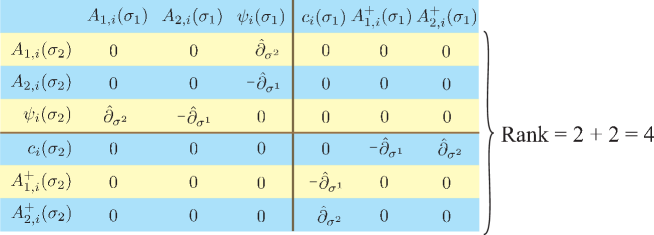
Figure 3: The Hessian matrix: $K[\Psi^{\alpha}(\sigma_{1}),\Psi^{\beta}(\sigma_{2})]:=\frac{\delta}{\delta\Psi^{\alpha}(\sigma_{2})}S\frac{\delta}{\delta\Psi^{\beta}(\sigma_{1})}$ The first column and first raw represent the right-hand side and the left-hand side of variation functions, respectively. $\hat{\partial}_{\sigma^{j}}:=\delta(\sigma-\sigma_{1})\partial_{\sigma^{j}}\delta(\sigma-\sigma_{2})$ represents a non-trivia Noether current ($j=1,2$). The Hessian is block diagonal matrix; the ranks of the upper left and the lower right parts are $2=3-1$. Therefore, the total rank of the Hessian is $2+2=4$ ($i$ is fixed).

Since $\sharp\Phi=4N$ (antifields will be fixed), the field number of the path-integral of $(S_{0})_{\rm gh}$ is equal to the rank of the Hessian of $(S_{0})_{\rm gh}$; hence, the path-integral of the action $(S_{0})_{\rm gh}$ become well-defined.

Finally, the gauge invariance action is written by

$$(S_{0})_{\rm gh}=S_{0}+\int_{\Sigma}(A^{i})^{+}\wedge\delta_{0}A_{i}$$ (143)

with $A_{i}:=A_{\mu,i}d\sigma^{\mu}$ and $\delta_{0}A_{\mu,i}=\partial_{\mu}\delta_{i}^{j}c_{j}$, where we define $\Phi^{+}_{\alpha}$ using a Hodge operator $*_{H}$: $\Phi^{+}_{\alpha}\equiv*_{\rm H}\Phi^{*}_{\alpha}$ (the definition of the Hodge operator is depend on the geometry of the disk $\Sigma$; we will introduce the explicit definition in section IV.4.2), which is also called as the anti-field.

IV.3.2 Condition of gauge invariance of classical action

In this section, we will add interaction terms: $S_{\rm gh}:=(S_{0})_{\rm gh}+g(S_{1})_{\rm gh}+\cdots$, where $g$ represents an expansion parameter, and we will see that $S_{\rm gh}$ is uniquely fixed except a certain two form $\alpha$ by a gauge invariance condition. Note that $\alpha$ satisfies the Jacobi’s identity. Therefore, we can identify $\alpha$ with the Poisson bracket.

First we discuss the gauge invariant condition. If we identify the fields and anti-fields with coordinates $q$ and canonical momentum $p$, i.e., $(\Phi^{\alpha_{i}},\Phi^{*}_{\alpha_{i}})\leftrightarrow(q^{\alpha_{i}},p_{\alpha_{i}})$, and we also identify the action $S$ and the Hamiltonian H: $S\leftrightarrow H$. In the analytical mechanics, $\delta_{\rm am}:=\{H,~{}\}$ represents a transform along the surface $H(q,p)={\rm constant}$, i.e., $\delta_{\rm am}$ holds the Hamiltonian. Similarly, we can define a gauge transformation, which holds the action $S$, using the Poisson bracket in the two-dimension field theory. It is known as the Batalin-Vilkovisky (BV) bracket Batalin198127 ; PhysRevD.28.2567 ; the definitions of the bracket are

$$\{f,g\}_{\rm BV}:=\sum_{\begin{subarray}{c}\alpha_{i}\\ i=0,1,\ldots\end{subarray}}\left(\frac{\delta f}{\delta\Phi^{\alpha_{i}}}\frac{\delta g}{\delta\Phi^{*}_{\alpha_{i}}}-\frac{\delta f}{\delta\Phi^{*}_{\alpha_{i}}}\frac{\delta g}{\delta\Phi^{\alpha_{i}}}\right)$$ (144)

with $f,~{}g\in C(\Psi)$.

The BV bracket has the ghost number $1$, then a BV-BRST operator $\delta_{\rm BV}:=\{S,~{}\}_{\rm BV}$ adds one ghost number. The BV bracket satisfies the following equations:

$$\{f,g\}_{\rm BV}=-(-1)^{({\rm gh}(f)+1)({\rm gh}(g)+1)}\{g,f\}_{\rm BV},$$ (145)

$$(-1)^{({\rm gh}(f)+1)({\rm gh}(h)+1)}\{f,\{g,h\}_{\rm BV}\}_{\rm BV}+{\rm cyclic}=0,$$ (146)

$$\{f,gh\}_{\rm BV}=\{f,g\}_{\rm BV}h+(-1)^{({\rm gh}(f)-1){\rm gh}(g)}g\{f,h\}_{\rm BV}$$ (147)

with $f,~{}g,~{}h\in C(\Psi)$.

Using the BV-BRST operator, the gauge invariance of action $S$ is written as $\delta_{\rm BV}S=0$, i.e.,

$$\{S,S\}_{BV}=0,$$ (148)

which is called the classical master equation. We use this equation and Eqs. (145) and (146); we obtain $\delta^{2}_{\rm BV}=0$, which corresponds to the condition of the BRST operator: $\delta^{2}_{\rm BRST}=0$ ($\delta_{\rm BRST}$ is the BRST operator). Therefore, the DV-BRST operator is the generalized BRST one.

Next, we discuss generalization of the topological field theory. Let us write a generalized action $S_{\rm gh}$ as

$$S_{\rm gh}=(S_{0})_{\rm gh}+g(S_{1})_{\rm gh}+g^{2}(S_{2})_{\rm gh}+\cdots,$$ (149)

where $g$ is an expansion parameter. Using gauge invariance condition (148), $(S_{n})_{\rm gh}$ ($n=1,2,\cdots$) is given by a solution of the following equation:

$$\left.\frac{\partial^{n}}{\partial g^{n}}\{S_{\rm gh},S_{\rm gh}\}_{\rm BV}\right|_{g=0}=0.$$ (150)

The general solution is given by Izawa

$$(S_{1})_{\rm gh} = \int_{\Sigma}d^{2}\sigma\Bigg{[}\frac{1}{2}\alpha^{ij}(A_{i}A_{j}-2\psi^{+}_{i}c_{j})+\frac{\partial\alpha^{ij}}{\partial\psi^{k}}\left(\frac{1}{2}(c^{+})^{k}c_{i}c_{j}-(A^{+})^{k}A_{i}c_{j}\right)$$ (151)

$$+\frac{1}{4}\frac{\partial^{2}\alpha^{ij}}{\partial\psi^{k}\partial\psi^{l}}(A^{+})^{k}(A^{+})^{l}c_{i}c_{j}\Bigg{]},$$

$$(S_{n>1})_{\rm gh} = 0$$ (152)

with $(A^{+})^{i}\equiv*_{\rm H}A_{\mu,i}^{*}=d\sigma^{\mu}\varepsilon_{\mu\nu}A_{\nu,i}^{*}$, $\psi^{+}_{i}\equiv*_{\rm H}\psi_{i}^{*}=\varepsilon_{\mu\nu}d\sigma^{\mu}\wedge d\sigma^{\nu}\psi^{*}_{i}$ and $(c^{+})^{i}\equiv*_{\rm H}(c^{*})^{i}=\varepsilon_{\mu\nu}d\sigma^{\mu}\wedge d\sigma^{\nu}(c^{*})^{i}$ ($\varepsilon_{\mu\nu}=-\varepsilon_{\nu\mu},~{}\varepsilon_{12}=1$), where $\alpha^{ij}$ is a function of $\psi$, and satisfies the following equation:

$$\frac{\partial\alpha^{ij}}{\partial\psi^{m}}\alpha^{mk}+\frac{\partial\alpha^{jk}}{\partial\psi^{m}}\alpha^{mi}+\frac{\partial\alpha^{kl}}{\partial\psi^{m}}\alpha^{mj}=0.$$ (153)

Here, if we identify $\psi^{i}$ with $x^{i}$, this equation is the Jacobi identity of Poisson bracket. Therefore, we can identify the Poisson bracket with the topological string theory.

IV.3.3 Gauge invariance in path integral

Now we discuss the path integral of the topological string theory $\int{\cal D}\Phi V(\Psi)$ with $V(\Psi)={\cal O}e^{\frac{i}{\hbar}S}$, and an observable quantity operator ${\cal O}$. Note that this path-integral does not include integrals in terms of the anti-fields. Therefore, we must fix the anti-fields; then, we consider that the anti-field $\Phi^{*}$ is a function of the field $\Phi$, i.e., $\Phi^{*}=\Omega(\Phi)$ and $\Omega\in{\cal C}(\Phi=\Psi)$ Namely, the path integral is defined by

$$\left.\int{\cal D}\Phi V(\Psi)\right|_{\Phi^{*}=\Omega}.$$ (154)

A choice of $\Omega(\Phi)$ is corresponding to the gauge fixing in the gauge theory. The path integral must be independent to the gauge choice (gauge invariance). To obtain a gauge invariant condition, we take the variation of the path integral in terms of anti-fields, and obtain the following gauge invariant condition Batalin1977309 :

$$\triangle_{\rm SD}V(\Psi)=0,$$ (155)

where we have introduced the Schwinger-Dyson (SD) operator:

$$\triangle_{\rm SD}:=\sum_{\alpha_{l}}(-1)^{\alpha_{l}}\frac{\delta}{\delta\Phi^{\alpha_{l}}}\frac{\delta}{\delta\Phi^{*}_{\alpha_{l}}},$$ (156)

where $(-1)^{\alpha_{l}}$ is defined as follows: if $\Phi^{\alpha_{l}}$ represents a boson, $(-1)^{\alpha_{l}}=(-1)^{{\rm gh}(\Phi^{\alpha_{l}})}$; if $\Phi^{\alpha_{l}}$ represents a fermion, $(-1)^{\alpha_{l}}=(-1)^{({\rm gh}(\Phi^{\alpha_{l}})+1)}$. Equation (155) is called the quantum master equation. It is known that the following two conditions are equivalence:

$$\triangle_{\rm SD}V(\Psi)=0\Longleftrightarrow\Omega=\frac{\overrightarrow{\delta}\varphi}{\delta\Phi^{a}},\ \ \ \exists\varphi,$$ (157)

where $\varphi$ is called the gauge-fixing fermion (an example will be shown later).

To perform the path integral, we generalize the classical action $S_{\rm gh}$ to a quantum action $W=S_{\rm gh}+{\rm i}\hbar W_{1}+({\rm i}\hbar)^{2}W_{2}+\cdots$. The correction terms $W_{n}$ ($n=1,2,\ldots$) are calculated from the master equation:

$$\triangle_{\rm SD}e^{\frac{i}{\hbar}W}=0,$$ (158)

or

$$\{S_{\rm gh},S_{\rm gh}\}_{\rm BV}=0,$$ (159)

$$\{W_{1},S_{\rm gh}\}_{\rm BV}+{\rm i}\hbar\triangle_{\rm SD}S_{\rm gh}=0,$$ (160)

$$\{W_{2},S_{\rm gh}\}_{\rm BV}+{\rm i}\hbar\triangle_{\rm SD}W_{1}+\frac{1}{2}\{W_{1},W_{1}\}_{\rm BV}=0,$$ (161)

$$\ \ \ \ \ \ \ \ \ \ \ \ \ \ \ \ \ \ \ \ \ \cdots$$

In the case where $\triangle_{\rm SD}S_{\rm gh}=0$, we can put $W_{1}=W_{2}=\cdots=0$. Fortunately, the topological string theory satisfies $\triangle_{\rm SD}S_{\rm gh}=0$. Therefore, we do not have to be concerned about the quantum correction of the action.

Finally, we consider the gauge fixing. Here we employ the Lorentz gauge:

$$d*_{\rm H}A_{i}=0,$$ (162)

and we add the integral of the Lorentz gauge to $S_{\rm gh}$. However, the path integral should hold gauge invariance, i.e., the path integral should be independent of gauge fixing term. Then, the gauge fixing can be written gauge-fixed fermion:

$$\varphi:=\int_{\Sigma}\gamma^{i}(d*_{\rm H}A_{i})=-\int_{\Sigma}d\gamma^{i}*_{\rm H}A_{i},$$ (163)

where we introduced $N$ fields $\gamma_{i}$ ($i=1,2,\ldots,N$), and anti-fields $\gamma_{i}^{+}$ are given by

$$\gamma^{+}_{i}=\frac{\overrightarrow{\partial}\varphi}{\partial\gamma_{i}}=d*_{\rm H}A_{i}.$$ (164)

Now, we employ the Lagrange multiplier method, and introduce $N$ scalar fields $\lambda_{i}$. The gauge-fixed action is written by

$$S_{\rm gf} = S_{\rm gh}-\int_{\Sigma}\gamma^{i}d*_{\rm H}A_{i}$$ (165)

$$= S_{\rm gh}-\int_{\Sigma}\lambda^{i}\gamma_{i}^{+}.$$ (166)

The other anti-fields are also fixed by this gauge-fixing fermion:

$$\psi^{+}_{i}=c^{+}_{i}=\lambda^{+}_{i}=0,$$ (167)

$$A^{+}_{i}=*_{\rm H}d\gamma^{i}.$$ (168)

Gauge fixed action $S_{\rm gf}$ is written by

$$S_{\rm gf} = \int_{\Sigma}\Bigg{[}A_{i}\wedge d\psi^{i}+\frac{1}{2}\alpha^{ij}A_{i}\wedge A_{j}-*_{\rm H}d\gamma^{i}\wedge\left(dc_{i}+\frac{\partial\alpha^{kl}}{\partial\psi^{i}}A_{k}c_{l}\right)$$ (169)

$$-\frac{1}{4}*_{\rm H}d\gamma^{i}\wedge*_{\rm H}d\gamma^{j}\frac{\partial^{2}\alpha^{kl}}{\partial\psi^{i}\partial\psi^{j}}c_{k}c_{l}-\lambda^{i}d*_{\rm H}A_{i}\Bigg{]}.$$

Here we perform the following variable transformations:

$$X^{i} := \psi^{i}+\theta^{\mu}A^{*}_{\mu}-\frac{1}{2}\theta^{\mu}\theta^{\nu}c^{+i}_{\mu}\nu,$$ (170)

$$\eta_{i} := c_{i}+\theta^{\mu}A_{i,\mu}+\frac{1}{2}\theta^{\mu}\theta^{\nu}\psi^{+}_{i,\mu\nu},$$ (171)

where $\theta^{\mu}\vartheta\nu=-\theta\nu\theta\mu$; ${\rm gh}(\theta^{\mu})=1$. For any scalar field $f(u)$ ($u\in\Sigma$), $\tilde{f}(u,\theta):=f(u)+\theta^{\mu}f^{(1)}_{\mu}(u)+\frac{1}{2}\theta^{\mu}\theta^{\nu}f^{(2)}_{\mu\nu}$ is called as the super field, where $f^{(1)}$ and $f^{(2)}$ represent a one-form field and a two-form field, respectively.

By using the super fields, the gauge fixed action $S_{\rm gf}$ can be rewritten as

$$S_{\rm gf}=\int_{\Sigma}\int d^{2}\theta\left[\eta_{i}DX^{i}-\lambda^{i}d*_{\rm H}A_{i}+\frac{1}{2}\alpha^{ij}(X)\eta_{i}\eta_{j}\right],$$ (172)

where $D:=\theta^{\mu}\frac{\partial}{\partial u^{\mu}}$. This is the final result in this section. Hereafter, we write $S^{0}_{\rm gf}:=\int_{\Sigma}\left[\eta_{i}DX^{i}-\lambda^{i}d*_{\rm H}A_{i}\right]$ and $S^{1}_{\rm gf}:=\int_{\Sigma}\alpha^{ij}\eta_{i}\eta_{j}/2$.

IV.4 Equivalence between deformation quantization and topological string theory

We return to the discussion about the deformation quantization. Here we see that the equivalence of the deformation quantization and the topological string theory, and introduce the perturbation theory of the topological string theory, which is equal to Kontsevich’s deformation quantization Kontsevich .

IV.4.1 Path integral as $L_{\infty}$ map

Here we summarize correspondence between Path integral with $L_{\infty}$ map.

First we note that the map: $\alpha:=\alpha(x)^{\mu\nu}\eta_{\mu}\eta_{\nu}/2\mapsto S_{\alpha}:=S^{1}_{\rm gf}=\int_{\Sigma}\alpha(x)^{\mu\nu}\eta_{\mu}\eta_{\nu}/2$ is isomorphic, because $\{S_{\alpha_{1}},S_{\alpha_{2}}\}_{\rm BV}=S_{\{\alpha_{1},\alpha_{2}\}_{\rm BV}}$.

SD operator satisfies the conditions of codifferential operator $Q$ in $L_{\infty}$ algebra, where the vector space and the degree of the space correspond to ${\cal C}(\Psi)$ and the ghost number, respectively.

The path integral $\int e^{\frac{i}{\hbar}S^{0}_{\rm gf}}$ gives the deformation quantization ${\mathscr{F}}_{0}+{\mathscr{F}}^{1}$. The master equation

$$Qe^{\frac{i}{\hbar}S_{\alpha}}=0$$ (173)

with $Q=\triangle_{\rm SD}$ is corresponding to the $L_{\infty}$ map’s condition $Q{\mathscr{F}}=0$

For $\alpha_{r}:=\alpha^{i_{1},i_{2},\cdots,i_{m}}\eta_{i_{1}}\eta_{i_{2}}\cdots\eta_{i_{m}}/m!$ with a positive integer $m$, ${\mathscr{F}}_{n}:V_{1}^{\otimes n}\otimes\rightarrow V_{2}$ is given by

$${\mathscr{F}}_{n}(\alpha_{1},\ldots,\alpha_{n})(f_{1}\otimes\cdots\otimes f_{m})(x):=\int e^{\frac{i}{\hbar}S^{0}}\frac{i}{\hbar}S_{\alpha_{1}}\cdots\frac{i}{\hbar}S_{\alpha_{n}}{\cal O}(f_{1},\ldots,f_{m}),$$ (174)

where $S_{\alpha_{r}}$ is the expansion of $S_{\alpha}$, and is defined as

$$S_{\alpha_{r}}:=\left.\left(\int_{\Sigma}\frac{1}{m!}\alpha^{i_{1}\cdots i_{m}}(X)\eta_{i_{1}}\cdots\eta_{i_{m}}\right)\right|_{\Phi^{*}=\partial\varphi},$$ (175)

and ${\cal O}$ is chosen to satisfy

$$Q\circ{\mathscr{F}}={\mathscr{F}}\circ Q,$$ (176)

where ${\mathscr{F}}:={\mathscr{F}}_{0}+{\mathscr{F}}^{1}+{\mathscr{F}}^{2}+\cdots$. We put ${\cal O}$ as follow:

$${\cal O}(f_{1},\ldots,f_{m}) = \int_{B_{m}}[X(t_{1},\theta_{1}))\cdots f_{m}(X(t_{m},\theta_{m}))]_{(m-2)}\delta_{x}(X(\infty)),$$ (177)

$$\equiv \int_{1=t_{1}>t_{2}>\cdots>t_{m}=0}f_{1}(\psi(1))\prod_{k=2}^{m-1}\partial_{i_{k}}\left[f(\psi(t_{k}))A^{+i_{k}}(t_{k})\right]f_{m}(\psi(0))\delta_{x}(\psi(\infty))$$ (178)

where the subscript ${(m-2)}$ denotes that $(m-2)$ forms are picked up from the products of super fields, and $B_{m}$ represents the surface of the disk $\Sigma$, i.e., $t$ is the parameter specifying the position on the boundary $\partial\Sigma$ ($1=t_{1}>t_{2}>\cdots>t_{m-1}>t_{m}=0)$.

To be exact, the action and fields include gauge fixing terms, ghost fields and anti-field. Finally, the deformation quantization is given as follow:

$$(f\star g)(x)=\int{\cal D}\Phi{f(\psi(1))g(\psi(0))\delta(x^{i}-\psi^{i}(\infty))}e^{\frac{i}{\hbar}S_{\rm gf}}.$$ (179)

IV.4.2 Perturbation theory

Now we see that the perturbation theory of the topological string theory. First, we write the action as $S_{\rm gf}=S^{0}_{\rm gf}+S^{1}_{\rm gf}$. The first term is defined as

$$S^{0}_{\rm gf}=\int_{\Sigma}\left[A_{i}\wedge(d\xi^{i}+*_{\rm H}d\lambda^{i})+c_{i}d*_{\rm H}d\gamma^{i}\right],$$ (180)

where $\xi^{i}\equiv\psi^{i}-x^{i}$, and we have expanded $\psi^{i}$ around $x^{i}$. The path integral of an observable quantity $\langle{\cal O}\rangle$ is given by

$$\int e^{\frac{i}{\hbar}S_{\rm gf}}{\cal O}=\sum_{n=0}^{\infty}\frac{i^{n}}{\hbar^{n}n!}\int e^{\frac{i}{\hbar}S^{0}_{\rm gf}}(S^{1}_{\rm gf})^{n}{\cal O},$$ (181)

where $\int:=\int{\cal D}\xi{\cal D}A{\cal D}c{\cal D}\gamma{\cal D}\lambda$. This expansion corresponds to the summation of all diagrams by the contractions of all pairs in terms of fields and ghost fields. From equation (180), propagators are inverses of

$$d\oplus*_{\rm H}d,\ \ \ \ d*_{\rm H}d.$$ (182)

Here we assume that the disk is the upper complex plane: $\Sigma=\{z~{}|~{}z=u+iv,~{}u,v\in\mathbb{R},~{}v\geq 0\}$ with $i^{2}=-1$, and the boundary is $\partial\Sigma=\{z~{}|~{}z=u,~{}u\in\mathbb{R}\}$. ($\mathbb{R}$ represents the real number space, and $z$ denotes a complex number.) The Hodge operator $*_{\rm H}$ is defined by

$$\left\{\begin{array}[]{c}*_{\rm H}du=dv\\ _{\rm H}dv=-du\end{array}\right.\longmapsto\left\{\begin{array}[]{c}*_{\rm H}dz=-idz\\ _{\rm H}d\overline{z}=id\overline{z}\end{array}\right.,$$ (187)

where $\overline{z}$ represents the complex conjugate of $z$. Moreover,

$$d_{z}=du\frac{\partial}{\partial u}+dv\frac{\partial}{\partial v}=dz\frac{\partial}{\partial z}+d\overline{z}\frac{\partial}{\partial\overline{z}},$$ (188)

$$\delta_{z}(w):=\delta(w-z)du_{w}\wedge dv_{w},~{}\int\delta_{z}(w)=1,$$ (189)

where $w\in\mathbb{C}$ with the complex number plane $\mathbb{C}$, and $w\equiv u_{w}+iv_{w}$.

Now, we calculate Green functions of $d\oplus*_{\rm H}d$ and $d*_{\rm H}d$, because the Green functions are inverses of these operators:

$$D_{w}G(z,w)={\rm i}\hbar\delta_{z}(w),$$ (190)

where $D_{w}=d_{w}\oplus*_{\rm H}d_{w}~{}{\rm or}~{}d_{w}*_{\rm H}d_{w}$. The solution depends on the boundary condition. In the case that $z$ and $w$ satisfy the Neumann boundary condition, a solution is a function of

$$\phi^{h}(z,w):=\frac{1}{2i}{\rm log}\frac{(z-w)(z-\overline{w})}{(\overline{z}-w)(\overline{z}-\overline{w})}.$$ (191)

On the other hand, $z$ and $w$ satisfy the Dirichlet boundary condition, a solution is a function of

$$\psi^{h}(z,w):=\log\left|\frac{z-w}{z-\overline{w}}\right|.$$ (192)

The Neumann boundary condition is $0=\partial_{u^{1}}G(z,w)|_{u^{2}=0}$, and the Dirichlet boundary condition is $0=\partial_{u^{2}}G(z,w)|_{u^{1}=0}$.

The propagators are given by

$$\langle\gamma^{k}(w)c_{j}(z)\rangle = \frac{{\rm i}\hbar}{2\pi}\delta^{k}_{j}\psi^{h}(z,w),$$ (193)

$$\langle\xi^{k}(w)A_{j}(z)\rangle = \frac{{\rm i}\hbar}{2\pi}\delta^{k}_{j}d_{z}\phi^{h}(z,w),$$ (194)

$$\langle(*_{\rm H}d\gamma^{k})(w)c_{j}(z)\rangle = \frac{{\rm i}\hbar}{2\pi}\delta^{k}_{j}\delta_{w}\phi^{h}(z,w),$$ (195)

and so on. From these propagators, we can obtain diagram rules corresponding to the deformation quantization. In section IV.5, we will introduce exact diagram rules.

To obtain the star product, we choice

$${\cal O}_{x}=f(X(1))g(X(0))\delta_{x}(\psi(\infty))$$ (196)

IV.5 Diagram rules of deformation quantization

From the perturbation theory of the topological string theory, we can obtain the following diagram rules of the star product, which is first given by Kontsevich Kontsevich ; Sugimoto :

$$(f\star g)(x)=f(x)g(x)+\sum^{\infty}_{n=1}\left(\frac{{\rm i}\hbar}{2}\right)^{n}\sum_{\Gamma\in G_{n}}w_{\Gamma}B_{\Gamma,\alpha}(f,g).$$ (197)

where $\Gamma$, $B_{\Gamma,\alpha}(f,g)$ and $w_{\Gamma}$ are defined as follows:

Definition. 1

$G_{n}$ is a set of the graphs $\Gamma$ which have $n+2$ vertices and $2n$ edges. Vertices are labeled by symbols “$1$”, “$2$”, $\ldots$ , “$n$”, “$L$”, and “$R$”. Edges are labeled by symbol $(k,v)$, where $k=1,2,\ldots,n$, $v=1,2,\ldots,n,L,R$, and $k\not=v$. $(k,v)$ represents the edge which starts at “$k$” and ends at “$v$”. There are two edges starting from each vertex with $k=1,2,\ldots,n$; $L$ and $R$ are the exception, i.e., they act only as the end points of the edges. Hereafter, $V_{\Gamma}$ and $E_{\Gamma}$ represent the set of the vertices and the edges, respectively.

Definition. 2

$B_{\Gamma,\alpha}(f,g)$ is the operator defined by:

$$B_{\Gamma,\alpha}(f,g) := \sum_{I:E_{\Gamma}\rightarrow\{i_{1},i_{2},\cdots,i_{2n}\}}\left[\prod^{n}_{k=1}\left(\prod_{e\in E_{\Gamma},e=(k,*)}\partial_{I(e)}\right)\alpha^{I((k,v_{k}^{1}),(k,v_{k}^{2}))}\right]\times$$ (198)

$$\left[\left(\prod_{e\in E_{\Gamma},e=(*,L)}\partial_{I(e)}\right)f\right]\times\left[\left(\prod_{e\in E_{\Gamma},e=(*,R)}\partial_{I(e)}\right)g\right],$$

where, $I$ is a map from the list of edges $((k,v_{k}^{1,2})),k=1,2,\ldots,n$ to integer numbers $\{i_{1},i_{2},\cdots,i_{2n}\}$. Here $1\leq i_{n}\leq d$; $d$ represents a dimension of the manifold $M$. $B_{\Gamma,\alpha}(f,g)$ corresponds to the graph $\Gamma$ in the following way: The vertices “$1$”, “$2$”, $\ldots$ , “$n$”, correspond to the Poisson structure $\alpha^{ij}$. $R$ and $L$ correspond to the functions $f$ and $g$, respectively. The edge $e=(k,v)$ represents the differential operator $\partial_{(i~{}{\rm or}~{}j)}$ acting on the vertex $v$.

The simplest diagram for $n=1$ is shown in Fig. $\ref{example}(a)$, which corresponds to the Poisson bracket: $\{f,g\}=\sum_{i_{1},i_{2}}\alpha^{i_{1}i_{2}}(\partial_{x^{i_{1}}}f)(\partial_{x^{i_{2}}}g)$. The higher order terms are the generalizations of this Poisson bracket.

Figure $\ref{example}(b)$ shows a graph $\Gamma_{{\rm ex.2}}$ with $n=2$ corresponding to the list of edges

$$((1,L),(1,R),(2,R),(2,3));$$ (199)

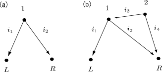
Figure 4: (a): The graph $\Gamma_{{\rm ex.1}}\in G_{1}$ corresponding to Poisson bracket. (b): A graph $\Gamma\in G_{2}$ correspond to the list of edges: $((1,L),(1,R),(2,R),(2,1))\mapsto\{i_{1},i_{2},i_{3},i_{4}\}$.

in addition, the operator $B_{\Gamma_{{\rm ex}.2},\alpha}$ is given by

$$(f,g)\mapsto\sum_{i_{1},\cdots,i_{4}}(\partial_{x^{i_{3}}}\alpha^{i_{1}i_{2}})\alpha^{i_{3}i_{4}}(\partial_{x^{i_{1}}}f)(\partial_{x^{i_{2}}}\partial_{x^{i_{4}}}g).$$ (200)

Definition. 3

We put the coordinates for the vertices in the upper-half complex plane $H_{+}:=\{z\in{\mathbb{C}}~{}|~{}{\rm Im}(z)>0\}$ $(\mathbb{C}$ represents the complex plain; ${\rm Im}(z)$ denotes the imaginary part of $z)$. Therefore, $R$ and $L$ are put at $0$ and $1$, respectively. We associate a weight $w_{\Gamma}$ with each graph $\Gamma\in G_{n}$ as

$$w_{\Gamma}:=\frac{1}{n!(2\pi)^{2n}}\int_{{\cal H}_{n}}\bigwedge_{k=1}^{n}\left(d\phi^{h}_{(k,v_{k}^{1})}\wedge d\phi^{h}_{(k,v_{k}^{2})}\right),$$ (201)

where $\phi$ is defined by

$$\phi^{h}_{(k,v)}:=\frac{1}{2i}{\rm Log}\left(\frac{(q-p)(\bar{q}-p)}{(q-\bar{p})(\bar{q}-\bar{p})}\right).$$ (202)

$p$ and $q$ are the coordinates of the vertexes “$k$” and “$v$”, respectively. $\bar{p}$ represents the complex conjugate of $p\in\mathbb{C}$. ${\cal H}_{n}$ denotes the space of configurations of $n$ numbered pair-wise distinct points on $H_{+}$:

$${\cal H}_{n}:=\{(p_{1},\cdots,p_{n})~{}|~{}p_{k}\in H_{+},~{}p_{k}\not=p_{l}~{}\text{for}~{}k\not=l\}.$$ (203)

Here we assume that $H_{+}$ has the metric:

$$ds^{2}=(d({\rm Re}(p))^{2}+d({\rm Im}(p))^{2})/({\rm Im}(p))^{2},$$ (204)

with $p\in H_{+}$; $\phi^{h}(p,q)$ is the angle which is defined by $(p,q)$ and $(\infty,p)$, i.e., $\phi^{h}(p,q)=\angle pq\infty$ with the metric $(\ref{eq:Metric})$. For example, $w_{\Gamma_{{\rm ex}.1}}$ corresponding to Fig. $\ref{example}(a)$ is calculated as:

$$w_{\Gamma_{{\rm ex}.1}}=\frac{2}{1!(2\pi)^{2}}\int_{{\cal H}_{1}}d\frac{1}{2i}{\rm Log}\left(\frac{p^{2}}{\overline{p}^{2}}\right)\wedge d\frac{1}{2i}{\rm Log}\left(\frac{(1-p)^{2}}{(1-\overline{p})^{2}}\right)=1,$$ (205)

where we have included the factor “$2$” arising from the interchange between two edges in $\Gamma$. $w_{\Gamma}$ corresponding to the Fig. $\ref{example}(b)$ is

$$w_{\Gamma_{(b)}} = \frac{1}{2!(2\pi)^{4}}\int_{{\cal H}_{2}}d\frac{1}{i}{\rm Log}\left(\frac{p_{1}}{\overline{p}_{1}}\right)\wedge d\frac{1}{i}{\rm Log}\left(\frac{1-p_{1}}{1-\overline{p}_{1}}\right)\wedge d\frac{1}{i}{\rm Log}\left(\frac{p_{2}}{\overline{p}_{2}}\right)\wedge d\frac{1}{2i}{\rm Log}\left(\frac{(p_{1}-p_{2})(\overline{p}_{1}-p_{2})}{(p_{1}-\overline{p}_{2})(\overline{p}_{1}-\overline{p}_{2})}\right)$$ (206)

$$= \frac{1}{2!(2\pi)^{4}}\int_{{\cal H}_{2}}d\frac{1}{i}{\rm Log}\left(\frac{p_{1}}{\overline{p}_{1}}\right)\wedge d\frac{1}{i}{\rm Log}\left(\frac{1-p_{1}}{1-\overline{p}_{1}}\right)$$

$$\wedge d\left(2\arg(p_{2})\right)\wedge d|p_{2}|\frac{\partial}{\partial|p_{2}|}\frac{1}{2i}{\rm Log}\left(\frac{(p_{1}-p_{2})(\overline{p}_{1}-p_{2})}{(p_{1}-\overline{p}_{2})(\overline{p}_{1}-\overline{p}_{2})}\right)$$

$$= \frac{1}{2!(2\pi)^{4}}\int_{{\cal H}_{2}}d\frac{1}{i}{\rm Log}\left(\frac{p_{1}}{\overline{p}_{1}}\right)\wedge d\frac{1}{i}{\rm Log}\left(\frac{1-p_{1}}{1-\overline{p}_{1}}\right)\wedge d\frac{1}{i}{\rm Log}\left(\frac{p_{2}}{\overline{p}_{2}}\right)\wedge d\frac{1}{i}{\rm Log}\left(\frac{1-p_{2}}{1-\overline{p}_{2}}\right)$$

$$= \frac{w_{1}^{2}}{2!}$$

$$= \frac{1}{2},$$

where $p_{1}$ and $p_{2}$ are the coordinates of vertexes “$1$” and “$2$”, respectively. Here, we have used the following facts:

$$\int_{0}^{\infty}d|p_{2}|\partial_{|p_{2}|}{\rm Log}\left(\frac{(p_{1}-p_{2})(\overline{p}_{1}-p_{2})}{(\overline{p}_{1}-p_{2})(\overline{p}_{1}-\overline{p}_{2})}\right) = \lim_{\Lambda\to\infty}{\rm Log}\left(\frac{(p_{1}-\Lambda e^{i\arg(p_{2})})(\overline{p}_{1}-\Lambda e^{i\arg(p_{2})})}{(p_{1}-\Lambda e^{-i\arg(p_{2})})(\overline{p}_{1}-\Lambda e^{-i\arg(p_{2})})}\right)$$

$$= \lim_{\Lambda\to\infty}{\rm Log}\left(\frac{(1-\Lambda e^{i\arg(p_{2})})(1-\Lambda e^{i\arg(p_{2})})}{(1-\Lambda e^{-i\arg(p_{2})})(1-\Lambda e^{-i\arg(p_{2})})}\right),$$

$$\int_{|p_{1}|>\Lambda}d{\rm Log}\left(\frac{p_{1}}{\overline{p}_{1}}\right)\wedge d{\rm Log}\left(\frac{1-p_{1}}{1-\overline{p}_{1}}\right) \stackrel{{\scriptstyle\Lambda\rightarrow\infty}}{{\longrightarrow}} \int_{|p_{1}|>\Lambda}d{\rm Log}\left(\frac{p_{1}}{\overline{p}_{1}}\right)\wedge d{\rm Log}\left(\frac{p_{1}}{\overline{p}_{1}}\right)=0.$$ (207)

Generally speaking, the integrals are entangled for $n\geq 3$ graphs, and the weight of these are not so easy to evaluate as Eq. $(\ref{w2})$.

Note that the above diagram rules also define the twisted element as the following relation: $(f\star g)\equiv\mu\circ{\cal F}(f\otimes g)$.

IV.6 Gauge invariant star product

From Eq. (77), the Poisson structure corresponding to our model is

$$\alpha^{ij}=\left(\begin{array}[]{ccc}0&\eta^{\mu\nu}&0\\ -\eta^{\mu\nu}&-q\hat{F}^{\mu\nu}&-q\epsilon^{abc}s^{a}A^{b}_{\mu}\\ 0&q\epsilon^{abc}s^{a}A^{b}_{\mu}&\epsilon^{abc}s^{c}\end{array}\right),$$ (211)

where the symbols $i$ and $j$ represent indexes of the phase space $(T\bm{X},\omega\bm{p},\bm{s})$. We separate the Poisson structure as follows:

$$\alpha := \left(\begin{array}[]{ccc}0&\eta^{\mu\nu}&0\\ -\eta^{\mu\nu}&0&0\\ 0&0&0\end{array}\right)+\left(\begin{array}[]{ccc}0&0&0\\ 0&0&-q\epsilon^{abc}A^{b}_{\mu}s^{a}\\ 0&q\epsilon^{abc}s^{a}A^{b}_{\mu}&\epsilon^{abc}s^{a}\end{array}\right)+\left(\begin{array}[]{ccc}0&0&0\\ 0&q\hat{F}^{\mu\nu}&0\\ 0&0&0\end{array}\right)$$ (221)

$$\equiv \alpha_{0}+\alpha_{A}+\alpha_{F}.$$ (222)

Here, for $f=f_{0}+f_{a}\sigma^{a}$, $\partial_{s^{a}}f:=f_{a}$ ($a=x,y,z$), where $f_{0,x,y,z}$ are functions $X$ and $p$. Because $\alpha_{0}$ is constant and $\alpha_{A}$ and $\alpha_{F}$ are functions of $X^{\mu}$ and $\bm{s}$, and any function $f$ is written as $f=f_{0}+\sum_{a=x,y,z}f_{a}s^{a}$ ($f_{0,a}$ only depends on $X$ and $p$), then we obtain additional diagram rules:

• Two edges starting from $\alpha_{F}$ connect with both vertices “$L$” and “$R$”.

• At least one edge from vertices $\alpha_{0}$ or $\alpha_{F}$ connect with vertices “$L$” or “$R$”.

• A number of the edges entering $\alpha_{A}$ is one or zero.

We also separate the graph $\Gamma$ into $\Gamma_{\alpha_{0}}$, $\Gamma_{\alpha_{A}}$ and $\Gamma_{\alpha_{F}}$. Here, we define the numbers of vertices $\alpha_{0}$, $\alpha_{A}$, and $\alpha_{F}$ as $n_{\alpha_{0}}$, $n_{\alpha_{A}}$, and $n_{\alpha_{F}}$, respectively. $\Gamma_{\alpha_{F}}$ is the graph consisted by vertices corresponding to $\alpha_{F}$, and “$L$” and “$R$”, and edges starting from these vertices. We consider $\Gamma_{\alpha_{F}}$ as a cluster, and define $\Gamma_{\alpha_{A}}$ as the graph consisted by the vertices corresponding to $\alpha_{A}$, which acts on the cluster corresponding to $\Gamma_{\alpha_{F}}$. $\Gamma_{\alpha_{0}}$ is the rest of the graph $\Gamma$ without $\Gamma_{\alpha_{A}}$ and $\Gamma_{\alpha_{F}}$. Here, we label vertexes $\Gamma_{\alpha_{F}}$, $\Gamma_{\alpha_{A}}$ and $\Gamma_{\alpha_{0}}$ by “$k=1-n_{\alpha_{F}}$”, “$k=(n_{\alpha_{F}}+1)-(n_{\alpha_{F}}+n_{\alpha_{A}})$” and “$k=(n_{\alpha_{F}}+n_{\alpha_{A}}+1)-(n_{\alpha_{F}}+n_{\alpha_{A}}+n_{\alpha_{0}})$”, respectively. The edge starting from “$k$” and ending to “$v_{k}^{1,2}$” represents $(k,v_{k}^{1,2})$.

Next, we calculate weight $w_{n_{\alpha_{F}}}$ and the operator $B_{\Gamma_{\alpha_{F}},\alpha_{F}}$ corresponding to $\Gamma_{\alpha_{F}}$, and later those for $\Gamma_{\alpha_{Aor0}}$.

Separation of graph $\Gamma$

We now sketch the proof of $w_{\Gamma}B_{\Gamma,\alpha}=w_{n_{\alpha_{0}}}B_{\Gamma_{\alpha_{0}},\alpha_{0}}\cdot w_{n_{\alpha_{A}}}B_{\Gamma_{\alpha_{A}},\alpha_{A}}\cdot w_{n_{\alpha_{F}}}B_{\Gamma_{\alpha_{F}},\alpha_{F}}$, where $w_{n_{\alpha_{a}}}=\frac{w_{1}^{n_{\alpha_{a}}}}{n_{\alpha_{a}}!}$ for $a=0,A,F$, and $w_{1}$ is given by Eq. (205).

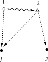
Figure 5: A four vertexes graph, where the white circle and the white square represent $\alpha_{A}$ and $\alpha_{F}$, respectively; the dotted arrow, waved arrow, and real arrow represent $\partial_{p}$, $\partial_{s}$, and $\partial_{X}$, respectively.

From the additional rule A1, each operator corresponding to vertexes $\alpha_{F}$ and edges $(\alpha_{F},L\ {\rm or}\ R)$ acts on $f$ and $g$ independently. Thus $w_{\alpha_{F}}\sim w_{1}^{n_{\alpha_{F}}}$. Secondly we consider the graph which consists of four vertexes corresponding to $\alpha_{A}$, $\alpha_{F}$, and “$L$”and “$R$” as shown in Fig. 5. We also assume that one edge of the vertex corresponding to $\alpha_{A}$ connects with a vertex corresponding to $\alpha_{F}$. In this case, from additional diagram rule A3, another edge of the vertex has to connect with “$L$” or “$R$”. Since we can exchange the role “$R$” and “$L$” by the variable transformation $p\mapsto 1-p$, ($p\in H_{+}$), we assume that one edge of the vertex corresponding to $\alpha_{A}$ connect with “$L$”. The weight $w_{\Gamma}$ in this case is given by Eq. (206), i.e., the integrals for the weight is given by replacing coordinate of the vertex corresponding to $\alpha_{F}$ with coordinate of “$R$” in $H_{+}$. This result can be expanded to every graph though a graph includes the vertices $\alpha_{0}$. For example, we illustrate the calculation of a six vertices graph, which only includes $\alpha_{0}$ and $\alpha_{F}$, in Fig. 6. At first we make the cluster having only vertices $\alpha_{F}$, $f$ and $g$ (fig. 6(b)), which is corresponding to the following operator: $\frac{w^{n_{\alpha_{F}}}}{n_{\alpha_{F}}!}\alpha_{F}^{i_{1}i_{2}}\alpha_{F}^{i_{3}i_{4}}(\partial_{p_{i_{1}}}\partial_{p_{i_{3}}}f)(\partial_{p_{i_{2}}}\partial_{p_{i_{4}}}g)$. The edges from the vertices act on the cluster independently (fig. 6(c)); we obtain the following operator: $\frac{w^{n_{\alpha_{0}}}}{n_{\alpha_{0}}!}\frac{w^{n_{\alpha_{F}}}}{n_{\alpha_{F}}!}\alpha^{j_{1}j_{2}}_{0}\alpha^{j_{3}j_{4}}_{0}(\partial_{X^{j_{1}}}\alpha_{F}^{i_{1}i_{2}})(\partial_{X^{j_{3}}}\alpha_{F}^{i_{3}i_{4}})(\partial_{X^{j_{2}}}\partial_{p_{i_{1}}}\partial_{p_{i_{3}}}f)(\partial_{X^{j_{4}}}\partial_{p_{i_{2}}}\partial_{p_{i_{4}}}g)$.

The position of each vertex corresponding to $\alpha_{A}$ and $\alpha_{F}$ can be move independently in integrals, and the entangled integral does not appear. Therefore the weight $w_{n_{\alpha_{A}}}$ of a graph $\Gamma_{\alpha_{A}}\sim w_{1}^{n_{\alpha_{A}}}$ only depends on the number of vertexes corresponding to $\alpha_{A}$ and $\alpha_{F}$, and $w_{\Gamma}=w_{n_{\alpha_{A}}}\cdot w_{n_{\alpha_{F}}}$ holds generally. From additional rule A2, we can similarly discuss about a graph $\Gamma_{\alpha_{0}}$, and obtain $w_{n_{\alpha_{0}}}\sim w_{1}^{n_{\alpha_{0}}}$. Finally, we can count the combination of $n_{\alpha_{0}}$, $n_{\alpha_{A}}$ and $n_{\alpha_{F}}$, and it is given by $\frac{(n_{\alpha_{0}}+n_{\alpha_{A}}+n_{\alpha_{F}})!}{(n_{\alpha_{A}}+n_{\alpha_{F}})!n_{\alpha_{0}}!}\cdot\frac{(n_{\alpha_{A}}+n_{\alpha_{F}})!}{n_{\alpha_{A}}!n_{\alpha_{F}}!}$. Therefore we obtain the Eq: $w_{\Gamma}B_{\Gamma,\alpha}=w_{n_{\alpha_{0}}}B_{\Gamma_{\alpha_{0}},\alpha_{0}}\cdot w_{n_{\alpha_{A}}}B_{\Gamma_{\alpha_{A}},\alpha_{A}}\cdot w_{n_{\alpha_{F}}}B_{\Gamma_{\alpha_{F}},\alpha_{F}}$.

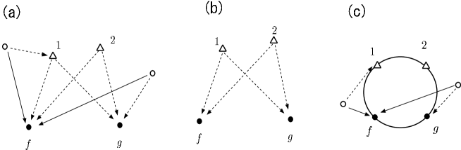
Figure 6: This figure shows the calculation method of the graph $(a)$, where the dotted arrow and real arrow represent the derivative with respect to $p$ and $X$, respectively, and the white circle and the white triangle represent $\alpha_{0}$ and $\alpha_{F}$, respectively. We rewrite the graph $(a)$ as the graph $(c)$ which is given by the cluster represented by the big circle and the operators into it, where the big circle represents the graph $(b)$.

The summation of each graph is easy, and we can derive the star product: $f\star g=\mu\circ{\cal F}_{A}(f\otimes g)$, where twisted element ${\cal F}_{A}$ is written as follow:

$${\cal F}_{A} = {\rm exp}\left\{\frac{{\rm i}\hbar}{2}\left(\partial_{X^{\mu}}\otimes\partial_{p_{\mu}}-\partial_{p\mu}\otimes\partial_{X^{\mu}}\right)\right\}$$ (223)

$$\circ\ {\rm exp}\left\{\frac{{\rm i}\hbar}{2}\varepsilon^{ijk}s^{k}\left(A_{\mu}^{i}\partial_{p_{\mu}}\otimes\partial_{s^{j}}+\partial_{s^{i}}\otimes\partial_{s^{j}}-\partial_{s^{j}}\otimes A_{\mu}^{i}\otimes\partial_{p_{\mu}}\right)\right\}$$

$$\circ\ {\rm exp}\left\{\frac{{\rm i}\hbar}{2}\left(F_{\mu\nu}^{a}s^{a}+F_{\mu\nu}\right)\partial_{p_{\mu}}\otimes\partial_{p_{\nu}}\right\}.$$

Because the action $I_{A}$ including a global U(1)$\times$SU(2) gauge field, the action $I_{A}$ is written as $I_{A}={\cal F}_{A}\circ{\cal F}_{0}^{-1}I_{0}$, thus, the map ${\cal F}_{0\mapsto A}:I_{0}\mapsto I_{A}$ is given by ${\cal F}_{0\mapsto A}={\cal F}_{A}\circ{\cal F}_{0}^{-1}$, i.e.,

$${\cal F}_{(0\mapsto A)} = {\rm exp}\left\{\frac{\mbox{i}\hbar}{2}\left(\partial_{X^{\mu}}\otimes\partial_{p_{\mu}}-\partial_{p\mu}\otimes\partial_{X^{\mu}}\right)\right\}$$ (224)

$$\circ\ {\rm exp}\left\{\frac{\mbox{i}\hbar}{2}\varepsilon^{ijk}s^{k}\left(A_{\mu}^{i}\partial_{p_{\mu}}\otimes\partial_{s^{j}}+\partial_{s^{i}}\otimes\partial_{s^{j}}-\partial_{s^{j}}\otimes A_{\mu}^{i}\otimes\partial_{p_{\mu}}\right)\right\}$$

$$\circ\ {\rm exp}\left\{\frac{\mbox{i}\hbar}{2}\left(F_{\mu\nu}^{a}s^{a}+F_{\mu\nu}\right)\partial_{p_{\mu}}\otimes\partial_{p_{\nu}}\right\}\circ{\rm exp}\left\{-\frac{\mbox{i}\hbar}{2}\varepsilon^{ijk}s^{k}\partial_{s^{i}}\otimes\partial_{s^{j}}\right\}$$

$$\circ\ {\rm exp}\left\{-\frac{\mbox{i}\hbar}{2}\left(\partial_{X^{\mu}}\otimes\partial_{p_{\mu}}-\partial_{X^{\mu}}\otimes\partial_{p_{\mu}}\right)\right\}.$$

The inverse map is given by the replacement of i by $-\mbox{i}$ in the map (224).

V Twisted spin

In this section, we will derive the twisted spin density, which corresponds to the spin density in commutative spacetime without the background SU(2) gauge field.

First, we will derive a general form of the twisted spin current in section V.1, which is written by using the twisted variation operator. This operator is constituted of the coproduct and twisted element; the coproduct reflects the action rule of the global SU(2) gauge symmetry generator, and the twisted element represents gauge structure of the background gauge fields.

In section V.2, at first, we will calculate the twisted spin density of the so-called Rashba-Dresselhaus model in the Wigner representation using the general form of the twisted spin density, and next, we will find the twisted spin operator in real spacetime using correspondence between operators in commutative spacetime and noncommutative phasespace.

V.1 Derivation of a twisted spin in Wigner space

The Lagrangian density in the Wigner space is given by

$${\cal L}(X,p)=\left(p_{0}-\frac{\bm{p}^{2}}{2m}\right)\star\left(\psi\psi^{\dagger}\right),$$ (225)

where $m$ is the electric mass, $f\star g:=\mu\circ{\cal F}_{A}(f\otimes g)$ for any functions $f$ and $g$.

The variation corresponding to the infinitesimal global SU(2) gauge transformation is defined as

$$\delta_{s^{a}}\psi = {\rm i}\vartheta s^{a}\psi,$$ (226)

$$\delta_{s^{a}}\psi^{\dagger} = -{\rm i}\psi^{\dagger}s^{a},$$ (227)

$$\delta_{s^{a}}x^{\mu} = 0,$$ (228)

where $\theta$ represents an infinitesimal parameter. Therefore, the variation of the Lagrangian density ${\cal L}(X,p):=\hat{\cal L}\star\psi\psi^{\dagger}$ is given by

$$\delta_{s^{a}}\left({\cal L}(X,p)\right):=\hat{\cal L}\star{\rm i}\theta s^{a}\star\psi\psi^{\dagger}-\hat{\cal L}\star\psi\psi^{\dagger}\star{\rm i}\theta s^{a}$$ (229)

Here we introduce the Grassmann numbers $\lambda_{1,2,3}$ ($\lambda_{3}:=\lambda_{1}\lambda_{2}$), the product $\mu$, and the coproduct $\triangle_{\eta}$, where the coproduct satisfies

$$\triangle_{\eta}(f):=f\otimes\eta+\eta\otimes f$$ (230)

for any functions $f$ and operator $\eta$. The equation (229) can be rewritten as

$$\delta_{s^{a}}\left({\cal L}\right) = \int d\lambda_{3}\mu\circ{\cal F}_{A}\left(\hat{\cal L}\otimes\left({\rm i}\lambda_{1}\theta s^{a}\star\lambda_{2}\psi\psi^{\dagger}+\lambda_{2}\psi\psi^{\dagger}\star{\rm i}\lambda_{1}\theta s^{a}\right)\right)$$ (231)

$$= \int d\lambda_{3}\mu\circ{\cal F}_{A}\left(\hat{\cal L}\otimes\mu\circ{\cal F}_{A}\triangle_{{\rm i}\lambda_{1}\theta s^{a}}\right)$$

$$= \int d\lambda_{3}\mu\circ{\cal F}_{A}({\rm id\otimes\mu})\circ({\rm id}\otimes{\cal F}_{A})\circ({\rm id}\otimes\triangle_{{\rm i}\lambda_{1}\theta s^{a}})\circ(\hat{\cal L}\otimes\lambda_{2}\psi\psi^{\dagger})$$

$$= {\rm i}\int d\lambda_{3}\mu\circ({\rm id}\otimes\mu)\circ({\rm id}\otimes\triangle){\cal F}_{A}\circ({\rm id}\otimes{\cal F}_{A})$$

$$\circ({\rm id}\circ\theta^{1/2}\otimes\theta^{1/2})\circ({\rm id}\otimes\triangle_{\lambda_{1}s^{a}})\circ(\hat{\cal L}\otimes\lambda_{2}\psi\psi^{\dagger}),$$

where we used $\int d\lambda_{i}\lambda_{j}=\delta_{ij}(i,j=1,2,3)$ with the Kronecker delta $\delta_{ij}$ Here we introduce the following symbols:

$$\hat{\mu} := \mu\circ({\rm id}\otimes\mu),$$ (232)

$$\hat{\cal F}_{A} := ({\rm id}\otimes\triangle){\cal F}_{A}\circ({\rm id}\otimes{\cal F}_{A}),$$ (233)

$$\hat{\theta} := \theta^{1/2}\otimes\theta^{1/2},$$ (234)

$$\hat{\triangle}_{\lambda_{1}s^{a}} := ({\rm id}\otimes\triangle_{\lambda_{1}s^{a}}),$$ (235)

where the coproduct in the differential operator space is defined as

$$\triangle(d_{n}):=\sum_{\begin{subarray}{c}i+j=n\\ i\geq 0,\ j\geq 0\end{subarray}}d_{i}\otimes d_{j}.$$ (236)

Here vectors $\{d_{0},d_{1},\dots\}$ corresponding to following operators: $d_{0}:={\rm id}$ and $d_{n}:=(1/n!)(\partial^{n}/\partial p^{n})$, or $d_{0}:={\rm id}$ and $d_{n}:=(1/n!)(\partial^{n}/\partial x^{n})$ ($n=1,2,\dots$), and $d_{l}$ are bases of a vector space $B(k):=\bigoplus_{l=0}^{\infty}kd_{l}$ ($k$ represents a scalar). The coproduct $\triangle$ in the vector space $B(k)$ satisfies the coassociation law: $(\triangle\otimes{\rm id})\otimes\triangle=({\rm id}\otimes\triangle)\circ\triangle$ because

$$(\triangle\otimes{\rm id})\circ\triangle(d_{n}) = \sum_{\begin{subarray}{c}i+j=n\\ i\geq 0,\ j\geq 0\end{subarray}}\triangle(d_{i})\otimes d_{j}$$ (237)

$$= \sum_{\begin{subarray}{c}i+j=n\\ i\geq 0,\ j\geq 0\end{subarray}}\left(\sum_{\begin{subarray}{c}k+l=i\\ k\geq 0,\ l\geq 0\end{subarray}}d_{k}\otimes d_{l}\otimes d_{j}\right)$$

$$= \sum_{\begin{subarray}{c}k+l+j=n\\ k\geq 0,\ l\geq 0,\ j\geq 0\end{subarray}}d_{k}\otimes d_{l}\otimes d_{j}$$

and

$$({\rm id}\otimes\triangle)\circ\triangle(d_{n}) = \sum_{\begin{subarray}{c}i+j=n\\ i\geq 0,\ j\geq 0\end{subarray}}d_{i}\otimes\triangle(d_{j})$$ (238)

$$= \sum_{\begin{subarray}{c}i+k+l=n\\ i\geq 0,\ k\geq 0,\ l\geq 0\end{subarray}}d_{i}\otimes d_{k}\otimes d_{l}.$$

It represents the Leibniz rule with respect to the differential operator $\partial_{\mu}$. For instance, $({\rm id}\otimes\triangle)(\partial_{\mu}\otimes\partial_{\nu}):=\partial_{\mu}\otimes\triangle(\partial_{\nu})=\partial_{\mu}\otimes\partial_{\nu}\otimes{\rm id}+\partial_{\mu}\otimes{\rm id}\otimes\partial_{\nu}$; it corresponds to the following calculation:

$$\partial_{\mu}f\cdot\partial_{\nu}(g\cdot h)=\partial_{\mu}f\cdot\partial_{\nu}g\cdot h+\partial_{\mu}f\cdot g\cdot\partial_{\nu}h.$$ (239)

The variation (231) is rewritten as

$$\delta_{s^{a}}{\cal L}(X,p)={\rm i}\int d\lambda_{3}\hat{\mu}\circ\hat{\cal F}_{A}\circ\hat{\theta}\circ\hat{\triangle}_{\lambda_{1}s^{a}}\circ(\hat{\cal L}\otimes\lambda_{2}\psi\psi^{\dagger}).$$ (240)

If we replace $\hat{\triangle}^{t}_{\lambda_{1}s^{a}}:=\hat{\cal F}_{A}^{-1}\hat{\triangle}_{\lambda_{1}s^{a}}{\cal F}_{0}$ with $\hat{\triangle}_{\lambda_{1}s^{a}}$ in equation (240), the integrals in terms of $x$ and $p$ of the right-hand side of Eq. (240) become zero because $\hat{\cal F}_{A}\circ\hat{\triangle}^{t}_{\lambda_{1}s^{a}}$ does not include the SU(2) field, which breaks the global SU(2) gauge symmetry, in the case that the parameter $\theta$ is constant. Therefore, for the action $S:=\int d^{\rm Dim}Xd^{\rm Dim}p{\cal L}(X,p)/(2\pi\hbar)^{\rm Dim}$,

$$\delta_{s^{a}}^{t}S:={\rm tr}\iiint d\lambda_{3}d^{\rm Dim}X\frac{d^{\rm Dim}p}{(2\pi\hbar)^{\rm Dim}}\hat{\mu}\circ\hat{\cal F}_{A}\circ\hat{\theta}\circ\hat{\triangle}^{t}_{\lambda_{1}s^{a}}(\hat{\cal L}\otimes\lambda_{2}\psi\psi^{\dagger})$$ (241)

is the infinitesimal SU(2) gauge transformation with background SU(2) gauge fields.

Because $\delta^{t}_{s^{a}}S=0$, we can write

$$\delta^{t}_{s^{a}}S=\int d^{\rm Dim}X\theta\left(\partial^{\mu}j^{t}_{\mu}\right).$$ (242)

In the case that the infinitesimal parameter depends on the spacetime coordinate, this equation can be written as

$$\delta^{t}_{s^{a}}S = \int d^{\rm Dim}X\theta(X)\left(\partial^{\mu}j^{t}_{\mu}\right)$$ (243)

$$= -\int d^{\rm Dim}X\left(\frac{\partial\theta(X^{\prime})}{\partial X^{\prime}_{\mu}}\right)j^{t}_{\mu}(X^{\prime}).$$

Therefore, we obtain the twisted Noether current

$$j^{t}_{\mu}=-\frac{\delta^{t}_{s^{a}}S}{\delta(\partial_{\mu}\theta(X))}.$$ (244)

In particular, the twisted spin

$$S^{t}_{a} = \int d\bm{X}j^{t}_{0}$$ (245)

$$= \int d\bm{X}\frac{\delta^{t}_{s^{a}}S}{\delta(\partial_{T}\theta)}$$

is conserved quantity. Here, we assumed that the SU(2) gauge is static one. However, we do not use this condition in the derivation of the twisted Noether charge and current density. Then, we can derive the virtual twisted spin with a time-dependent SU(2) gauge: $\tilde{S}^{t}_{a}$. In this case, we only use the time-dependent SU(2) gauge field strength $F^{a}_{\mu\nu}$, which has non-zero space-time components $F^{a}_{0i}$ ($i=1,2,\dots,{\rm Dim}-1$).

Here, we discuss the adiabaticity of the twisted spin. In the case that SU(2) gauge fields have time dependence, the twisted spin is not conserved. Now, we assume that $A^{a}_{\mu}=\lambda(t)C^{a}_{\mu}$ ($a=x,y,z$) with constant fields $C^{a}_{\mu}=(0,\bm{C}^{a})$; $\lambda(t)$ is an adequate slowly function dependent on time. Because $\tilde{S}^{t}_{a}$ includes $F_{\mu\nu}^{-1}\sim\frac{1}{(1+(\dot{\lambda})^{2}\bm{C}\cdot\bm{C})}\left(\begin{array}[]{cc}0&\dot{\lambda}\bm{C}\\ -\dot{\lambda}\bm{C}&\lambda^{-2}[\bm{C}_{i},\bm{C}_{j}]^{-1}\end{array}\right)$ with $\dot{\lambda}\equiv d\lambda/dt$, the difference between $\tilde{S}^{t}_{a}$ and $S^{t}_{a}$ comes from only that between inverse of field strength: $\Delta F^{-1}\sim\frac{1}{1+(\dot{\lambda})^{2}}\lambda^{-2}[C_{i},C_{j}]^{-1}-\lambda^{-2}[C_{i},C_{j}]^{-1}\sim(\dot{\lambda}/\lambda)^{2}[C_{i},C_{j}]^{-1}$. Therefore we obtain

$$\frac{dS^{t}_{a}}{dt}={\cal O}(\dot{\lambda}^{2}).$$ (246)

This means that $S^{t}_{a}$ is the adiabatic invariance. Namely, for the infinitely slow change in $\lambda(t)$ during the time period $T(\rightarrow\infty)$, $S^{t}_{a}$ remains constant while $\Delta\lambda=\lambda(T)-\lambda(0)$ is finite. This fact is essential for the spin-orbit echo proposed in Sugimoto2 .

V.2 Rashba-Dresselhaus model

Here we apply the formalism developed so far to an explicit model, i.e., the so-called Rashba-Dresselhaus model given by

$$H=\frac{\hat{\bm{p}}^{2}}{2m}+\alpha(\hat{p}_{x}\hat{\sigma}_{y}-\hat{p}_{y}\hat{\sigma}_{x})+\beta(\hat{p}_{x}\hat{\sigma}_{x}-{\hat{p}}_{y}\hat{\sigma}_{y})+V(\hat{x})$$ (247)

with a potential $V(\hat{x})$, where $\alpha$ and $\beta$ are the Rashba and Dresselhaus parameters, respectively. Completing square in terms of $\hat{p}$, we obtain $A^{x}_{x}=-2m\beta/(\hbar q)$, $A^{y}_{x}=-2m\alpha/(\hbar q)$, $A^{x}_{y}=2m\alpha/(\hbar q)$, $A^{y}_{y}=2m\beta/(\hbar q)$, $A_{0}=m(\alpha^{2}+\beta^{2})/e$, and $A^{z}_{x,y}=A^{x,y}_{z}=A^{z}_{z}=A_{0}^{x,y,z}=A_{x,y,z}=0$, where $q=|e|/(mc^{2})$.

To calculate the twisted symmetry generator $\hat{\triangle}^{t}(\lambda_{2}s^{a})$, we first consider the $\hat{{\cal F}}_{0}$. $({\rm id}\otimes\triangle){\cal F}_{0}$ is given by

$$({\rm id}\otimes\triangle){\cal F}_{0} = \exp\left\{\frac{{\rm i}\hbar}{2}\Big{(}\partial_{X^{\mu}}\otimes 1\otimes\partial_{p_{\mu}}+\partial_{X^{\mu}}\otimes\partial_{p_{\mu}}\otimes 1-\partial_{p_{\mu}}\otimes 1\otimes\partial_{X^{\mu}}-\partial_{p_{\mu}}\otimes\partial_{X^{\mu}}\otimes 1\Big{)}\right.$$ (248)

$$\left.+\frac{i}{2}\varepsilon^{ijk}\Big{(}s_{k}\partial_{s_{i}}\otimes 1\otimes\partial_{s_{j}}+s_{k}\partial_{s_{i}}\otimes\partial_{s_{j}}\otimes 1\Big{)}\right\},$$

and $\hat{\cal F}_{0}$ is given by

$$\hat{\cal F}_{0} = \exp\left\{\frac{{\rm i}\hbar}{2}\Big{(}\partial_{X^{\mu}}\otimes 1\otimes\partial_{p_{\mu}}+\partial_{X^{\mu}}\otimes\partial_{p_{\mu}}\otimes 1-\partial_{p_{\mu}}\otimes 1\otimes\partial_{X^{\mu}}-\partial_{p_{\mu}}\otimes\partial_{X^{\mu}}\otimes 1\Big{)}\right.$$ (249)

$$\left.+\frac{i}{2}\varepsilon^{ijk}\Big{(}s_{k}\partial_{s_{i}}\otimes 1\otimes\partial_{s_{j}}+s_{k}\partial_{s_{i}}\otimes\partial_{s_{j}}\otimes 1\Big{)}\right\}$$

$$\circ\exp\left\{\frac{{\rm i}\hbar}{2}\Big{(}1\otimes\partial_{X^{\mu}}\otimes\partial_{p_{\mu}}-1\otimes\partial_{p_{\mu}}\otimes\partial_{X^{\mu}}\Big{)}\right.$$

$$\left.+\frac{i}{2}\varepsilon^{ijk}\Big{(}1\otimes s_{k}\partial_{s_{i}}\otimes\partial_{s_{j}}\Big{)}\right\}$$

$$= \exp\left\{\frac{{\rm i}\hbar}{2}\Big{(}1\otimes\partial_{X^{\mu}}\otimes\partial_{p_{\mu}}+\partial_{X^{\mu}}\otimes 1\otimes\partial_{p_{\mu}}+\partial_{X^{\mu}}\otimes\partial_{p_{\mu}}\otimes 1\right.$$

$$\left.-1\otimes\partial_{p_{\mu}}\otimes\partial_{X^{\mu}}-\partial_{p_{\mu}}\otimes 1\otimes\partial_{X^{\mu}}-\partial_{p_{\mu}}\otimes\partial_{X^{\mu}}\otimes 1\Big{)}\right.$$

$$\left.+\frac{i}{2}\varepsilon^{ijk}\Big{(}1\otimes s_{k}\partial_{s_{i}}\otimes\partial_{s_{j}}+s_{k}\partial_{s_{i}}\otimes 1\otimes\partial_{s_{j}}+s_{k}\partial_{s_{i}}\otimes\partial_{s_{j}}\otimes 1\Big{)}\right\}$$

$$\equiv {\cal G}_{0}.$$

Similarly, $\hat{\cal F}_{A}$ is given by

$$\hat{\cal F}_{A} = \exp\left\{\frac{{\rm i}\hbar}{2}\Big{(}1\otimes\partial_{X^{\mu}}\otimes\partial_{p_{\mu}}+\partial_{X^{\mu}}\otimes 1\otimes\partial_{p_{\mu}}+\partial_{X^{\mu}}\otimes\partial_{p_{\mu}}\otimes 1\right.$$ (250)

$$\left.-1\otimes\partial_{p_{\mu}}\otimes\partial_{X^{\mu}}-\partial_{p_{\mu}}\otimes 1\otimes\partial_{X^{\mu}}-\partial_{p_{\mu}}\otimes\partial_{X^{\mu}}\otimes 1\Big{)}\right\}$$

$$\circ\exp\left\{\frac{i}{2}\varepsilon^{ijk}\Big{(}1\otimes s_{k}\partial_{s_{i}}\otimes\partial_{s_{j}}+s_{k}\partial_{s_{i}}\otimes 1\otimes\partial_{s_{j}}+s_{k}\partial_{s_{i}}\otimes\partial_{s_{j}}\otimes 1\right.$$

$$+1\otimes s^{k}A^{i}_{\mu}\partial_{p_{\mu}}\otimes\partial_{s^{j}}+s^{k}A^{i}_{\mu}\partial_{p_{\mu}}\otimes 1\otimes\partial_{s^{j}}+s^{k}A^{i}_{\mu}\partial_{p_{\mu}}\otimes\partial_{s^{j}}\otimes 1$$

$$\left.-1\otimes\partial_{s^{j}}\otimes s^{k}A^{i}_{\mu}\partial_{p_{\mu}}-\partial_{s^{j}}\otimes 1\otimes s^{k}A^{i}_{\mu}\partial_{p_{\mu}}-\partial_{s^{j}}\otimes s^{k}A^{i}_{\mu}\partial_{p_{\mu}}\otimes 1\Big{)}\right\}$$

$$\circ\exp\left\{\frac{{\rm i}\hbar}{2}\Big{(}1\otimes\hat{F}_{\mu\nu}\partial_{p_{\mu}}\otimes\partial_{p_{\nu}}+\hat{F}_{\mu\nu}\partial_{p_{\mu}}\otimes 1\otimes\partial_{p_{\nu}}+\hat{F}_{\mu\nu}\partial_{p_{\mu}}\otimes\partial_{p_{\nu}}\otimes 1\Big{)}\right\}$$

$$\equiv {\cal G}^{A}_{Xp}\circ{\cal G}^{A}_{sp}\circ{\cal G}^{A}_{pp}.$$

We note that the operators ${\cal G}_{0}~{}{\rm and}~{}{\cal G}^{A}_{Xp,sp,pp}$ have each inverse operator, which are denoted by $\overline{\cal G}_{0}~{}{\rm and}~{}\overline{\cal G}^{A}_{Xp,sp,pp}$, respectively. Here, the overline $-$ represents the complex conjugate.

Because the twisted variation is $\hat{\mu}\circ\hat{\cal F}_{A}\circ\hat{\theta}\circ\hat{\cal F}^{-1}_{A}\circ\hat{\triangle}_{\lambda_{1}s^{a}}\circ{\cal F}_{0}({\cal L}\otimes\lambda_{2}\psi\psi^{\dagger})$, the infinitesimal parameter $\hat{\theta}$ becomes an operator $\hat{\cal F}_{A}\circ\hat{\theta}\circ\hat{\cal F}^{-1}_{A}$. It is calculated by using the operator formula

$$e^{B}Ce^{-B}=\sum_{n=0}^{\infty}\frac{1}{n!}\underbrace{[B,[B,\cdots[B,}_{n}C]\cdots]]$$ (251)

for any operators $B$ and $C$. In the calculation, one will use the following formula in midstream:

$$\sum_{l=0}\frac{D^{l}}{(l+1)!} = \int_{0}^{1}d\lambda e^{\lambda D},$$ (252)

$$\sum_{l=0}\frac{D^{l}}{(l+2)!} = \int_{0}^{1}d\lambda\int_{0}^{\lambda}d\lambda^{\prime}e^{\lambda^{\prime}D},$$ (253)

and so on, for any operator $D$.

From these results of the calculations, we obtain the twisted spin as follow

$$s^{t}_{a}=\mu\circ{\cal F}_{A}\circ(s^{a}\otimes{\rm id})\circ\tilde{\Upsilon}\circ({\rm id}\otimes G)\circ\tilde{\Upsilon}^{\dagger},$$ (254)

where $\tilde{\Upsilon}$ is defined as

$$\tilde{\Upsilon} := \frac{1}{2}\left[e^{\frac{{\rm i}}{2}(\alpha+\beta)\sigma_{-}\big{(}\partial_{p_{x}}+\partial_{p_{y}}\big{)}}\otimes e^{\frac{{\rm i}}{2}(\alpha-\beta)\sigma_{+}\big{(}\partial_{p_{x}}-\partial_{p_{y}}\big{)}}\right]\circ\left[e^{-\frac{{\rm i}}{2}\big{(}{\partial_{X}}\otimes\partial_{Y}+{\partial_{Y}}\otimes\partial_{X}\Big{)}\circ\big{(}\frac{1}{2m(\alpha^{2}-\beta^{2})}\otimes\sigma^{z}\big{)}}\right.$$ (255)

$$\left.+e^{-\frac{{\rm i}}{2}\big{(}{\partial_{X}}\otimes\partial_{Y}+{\partial_{Y}}\otimes\partial_{X}\Big{)}\circ\big{(}\sigma^{z}\otimes\frac{1}{2m(\alpha^{2}-\beta^{2})}\big{)}}\right]+e^{\frac{{\rm i}}{2}(\alpha+\beta)\sigma_{-}\big{(}\partial_{p_{x}}+\partial_{p_{y}}\big{)}}\otimes\sin^{2}\left(\frac{{\rm i}\hbar\big{(}\partial_{X}-\partial_{Y}\big{)}}{8\sqrt{2}m(\alpha+\beta)}\right),$$

where $\sigma_{\pm}:=\sigma_{x}\pm\sigma_{y}$.

Finally, we will rewrite the twisted spin as an operator form in commutative spacetime. Roughly speaking, the operator in the commutative spacetime. and the one in the noncommutative Wigner space have the following relations (the left-hand side represents operators on the Wigner space; the right-hand side represents operators on the commutative spacetime):

$$X^{\mu}\star \Leftrightarrow \hat{x}^{\mu},$$ (256)

$$p_{\mu}\star \Leftrightarrow \hat{p}_{\mu},$$ (257)

$$s^{a}\star \Leftrightarrow \hat{s}^{a},$$ (258)

$${\rm i}\hbar\partial_{p_{\mu}}\star \Leftrightarrow \hat{x}^{\mu},$$ (259)

$$-{\rm i}\hbar\partial_{X^{\mu}}\star \Leftrightarrow \hat{p}_{\mu},$$ (260)

because $[X^{\mu},p_{\nu}]_{\star}:=X^{\mu}\star p_{\nu}-p_{\nu}\star X^{\mu}={\rm i}\hbar\delta_{\nu}^{\mu}$ is equal to the commutation of the operator form: $[\hat{x}^{\mu},\hat{p}_{\nu}]={\rm i}\hbar\delta_{\nu}^{\mu}$. The equivalence of $s^{t}_{a}$ and the twisted spin in the operator form on the commutative spacetime $\hat{s}^{t}_{a}$ can be confirmed using the Wigner transformation in terms of $\hat{s}^{t}_{a}$.

The operator form of the twisted spin is given by

$$s^{t}_{a}=\frac{\hbar}{2}\psi^{\dagger}\Upsilon^{\dagger}\sigma^{a}\Upsilon\psi,$$ (261)

where

$$\Upsilon = \lim_{x^{\prime}\rightarrow x}\frac{1}{2}e^{\frac{{\rm i}}{2}m(\alpha+\beta)\sigma_{-}x_{+}}\left[e^{-\frac{{\rm i}}{2}m(\alpha-\beta)\sigma_{+}x^{\prime}_{-}}e^{-\frac{{\rm i}}{2}\frac{\sigma^{z}}{2m^{2}(\alpha^{2}-\beta^{2})}\big{(}\overleftarrow{\partial}_{x^{\prime}}\partial_{y}+\overleftarrow{\partial}_{y^{\prime}}\partial_{x}\big{)}}\right.$$ (262)

$$\left.+e^{-\frac{{\rm i}}{2}\frac{\sigma^{z}}{2m^{2}(\alpha^{2}-\beta^{2})}\big{(}\partial_{x^{\prime}}\partial_{y}+\partial_{y^{\prime}}\partial_{x}\big{)}}e^{-\frac{{\rm i}}{2}m(\alpha-\beta)\sigma_{+}x^{\prime}_{-}}+2\sin^{2}\left(\frac{{\rm i}\hbar(\partial_{x}-\partial_{y})}{8\sqrt{2}m(\alpha+\beta)}\right)\right]$$

with $x_{\pm}:=x\pm y$.

This operator in Eq. (261), when integrated over $\bm{X}$, is the conserved quantity for any potential configuration $V(\hat{x})$ as long as $\alpha$, $\beta$ are static and the electron-electron interaction is neglected.

VI Conclusions

In this paper, we have derived the conservation of the twisted spin and spin current densities. Also the adiabatic invariant nature of the total twisted spin integrated over the space is shown. Here we remark about the limit of validity of this conservation law. First, we neglected the dynamics of the electromagnetic field $A_{\mu}$ which leads to the electron-electron interaction. This leads to the inelastic electron scattering, which is not included in the present analysis, and most likely gives rise to the spin relaxation. This inelastic scattering causes the energy relaxation and hence the memory of the spin will be totally lost after the inelastic lifetime. This situation is analogous to the two relaxation times $T_{1}$ and $T_{2}$ in spin echo in NMR and ESR. Namely, the phase relaxation time $T_{2}$ is usually much shorter than the energy relaxation time $T_{1}$, and the spin echo is possible for $T<T_{1}$. Similar story applies to spin-orbit echo Sugimoto2 where the recovery of the spin moment is possible only within the inelastic lifetime of the spins. However, the generalization of the present study to the dynamical $A_{\mu}$ is a difficult but important issue left for future investigations. Also the effect of the higher order terms in $1/(mc^{2})$ in the derivation of the effective Lagrangian from Dirac theory requires to be scrutinized.

Another direction is to explore the twisted conserved quantities in the non-equilibrium states. Under the static electric field, the system is usually in the current flowing steady state. Usually this situation is described by the linear response theory, but the far from equilibrium states can in principle be described by the non-commutative geometry SOnoda ; Sugimoto . The nonperturbative effects in this non-equilibrium states are the challenge for theories, and deserve the further investigations.

The author thanks Y.S. Wu, F.C. Zhang, K. Richter, V. Krueckl, J. Nitta, and S. Onoda for useful discussions. This work was supported by Priority Area Grants, Grant-in-Aids under the Grant number 21244054, Strategic International Cooperative Program (Joint Research Type) from Japan Science and Technology Agency, and by Funding Program for World-Leading Innovative R and D on Science and Technology (FIRST Program).

References

- (1) M. E. Peshkin and D. V. Schroeder. Introduction to Quantum Field Theory. Addison-Wesley, New York (1995).
- (2) J. Fröhlich and U. M. Studer. Gauge invariance and current algebra in nonrelativistic many-body theory. Rev. Mod. Phys., 65, 733–802 (1993).
- (3) G. Volovik. The Universe in a Helium Droplet. Oxford University Press, Oxford, U.K. (2003).
- (4) B. Leurs, Z. Nazario, D. Santiago and J. Zaanen. Non-Abelian hydrodynamics and the flow of spin in spin–orbit coupled substances. Annals of Physics, 323(4), 907 – 945 (2008).
- (5) N. Seiberg and E. Witten. String theory and noncommutative geometry. Journal of High Energy Physics, 09, 032 (1999).
- (6) M. Chaichian, P. Kulish, K. Nishijima and A. Tureanu. On a Lorentz-invariant interpretation of noncommutative space-time and its implications on noncommutative QFT. Physics Letters B, 604(1-2), 98–102 (2004).
- (7) M. Chaichian, P. Prešnajder and A. Tureanu. New Concept of Relativistic Invariance in Noncommutative Space-Time: Twisted Poincaré Symmetry and Its Implications. Phys. Rev. Lett., 94, 151602 (2005).
-
(8)
G. Amelino-Camelia, G. Gubitosi, A. Marcianò, P. Martinetti, F. Mercati,
D. Pranzetti and R. A. Tacchi.
First Results of the Noether Theorem
for Hopf-Algebra Spacetime Symmetries. Progress of Theoretical Physics Supplement, 171, 65–78 (2007). - (9) G. Amelino-Camelia, G. Gubitosi, A. Marcianò, P. Martinetti and F. Mercati. A no-pure-boost uncertainty principle from spacetime noncommutativity. Physics Letters B, 671(2), 298–302 (2009).
- (10) S. Maekawa. Concepts in Spin Electronics. OXFORD SCIENCE PUBLICATIONS (2006).
- (11) N. Sugimoto and N. Nagaosa. Spin-orbit echo. To apper in Science.
- (12) E. L. Hill. Hamilton’s Principle and the Conservation Theorems of Mathematical Physics. Rev. Mod. Phys., 23, 253–260 (1951).
- (13) C. Gonera, P. Kosiński, P. Maślanka and S. Giller. Space-time symmetry of noncommutative field theory. Physics Letters B, 622(1-2), 192–197 (2005).
- (14) E. Wigner. On the Quantum Correction For Thermodynamic Equilibrium. Phys. Rev., 40, 749–759 (1932).
- (15) J. E. Moyal. Mathematical Proceedings of the Cambridge Philosophical Society. Proc. Cambridge Phil. Soc., 45, 99–124 (1949).
-
(16)
S. Onoda, N. Sugimoto and N. Nagaosa.
Theory of Non-Equilibirum States
Driven by Constant Electromagnetic Fields. Progress of Theoretical Physics, 116(1), 61–86 (2006). - (17) M. Kontsevich. Deformation Quantization of Poisson Manifolds. Letters in Mathematical Physics, 66, 157–216 (2003).
- (18) F. Bayen, M. Flato, C. Fronsdal, A. Lichnerowicz and D. Sternheimer. Deformation theory and quantization. I. Deformations of symplectic structures. Annals of Physics, 111(1), 61 – 110 (1978).
- (19) F. Bayen, M. Flato, C. Fronsdal, A. Lichnerowicz and D. Sternheimer. Deformation theory and quantization. II. Physical applications. Annals of Physics, 111(1), 111 – 151 (1978).
- (20) G. Hochschild. On the Cohomology Groups of an Associative Algebra. The Annals of Mathematics, 46(1), pp. 58–67 (1945).
- (21) D. Happel. Hochschild cohomology of finite—dimensional algebras. In M.-P. Malliavin, editor, Séminaire d’Algèbre Paul Dubreil et Marie-Paul Malliavin, vol. 1404 of Lecture Notes in Mathematics, pages 108–126. Springer Berlin / Heidelberg. ISBN 978-3-540-51812-9 (1989).
- (22) M. Gerstenhaber. The Cohomology Structure of an Associative Ring. The Annals of Mathematics, 78(2), 267–288 (1963).
- (23) E. Cartan. Sur la structure des groupes infinis de transformation. Annales Scientifiques de l’École Normale Supérieure, 22, 219–308 (0012-9593).
- (24) A. S. Cattaneo and G. Felder. A Path Integral Approach to the Kontsevich Quantization Formula. Communications in Mathematical Physics, 212, 591–611 (2000).
- (25) N. Ikeda and I. Ken-iti. Dimensional reduction of nonlinear gauge theories. Journal of High Energy Physics, 09, 030 (2004).
- (26) I. A. Batalin and G. A. Vilkovisky. Gauge algebra and quantization. Physics Letters B, 102(1), 27–31 (1981).
- (27) I. A. Batalin and G. A. Vilkovisky. Quantization of gauge theories with linearly dependent generators. Phys. Rev. D, 28, 2567–2582 (1983).
- (28) J. Alfaro and P. Damgaard. Origin of antifields in the Batalin-Vilkovisky lagrangian formalism. Nuclear Physics B, 404(3), 751–793 (1993).
- (29) I. Batalin and G. Vilkovisky. Relativistic S-matrix of dynamical systems with boson and fermion constraints. Physics Letters B, 69(3), 309–312 (1977).
- (30) N. Sugimoto, S. Onoda and N. Nagaosa. Gauge Covariant Formulation of the Wigner Representation through Deformation Quantization. Progress of Theoretical Physics, 117(3), 415–429 (2007).