Planar Ising magnetization field I. Uniqueness of the critical scaling limit

Abstract

The aim of this paper is to prove the following result. Consider the critical Ising model on the rescaled grid $a\mathbb{Z}^{2}$, then the renormalized magnetization field

$$\Phi^{a}:=a^{15/8}\sum_{x\in a\mathbb{Z}^{2}}\sigma_{x}\delta_{x},$$

seen as a random distribution (i.e., generalized function) on the plane, has a unique scaling limit as the mesh size $a\searrow 0$. The limiting field is conformally covariant.

,
and

T1Supported in part by NWO Grant Vidi 639.032.916. T2Supported in part by ANR Grant MAC2 10-BLAN-0123. T3Supported in part by NSF Grants OISE-0730136 and DMS-10-07524.

1 Introduction

1.1 Overview

The Ising model, introduced by Lenz in 1920 to describe ferromagnetism, is one the most studied models of statistical mechanics. Its two-dimensional version has played a special role in the theory of critical phenomena since Peierls famously proved, in 1936, that it undergoes a phase transition, and Onsager presented, in 1944, his derivation of the free energy Onsager . The phase transition of the two-dimensional Ising model has been extensively studied by both physicists and mathematicians, becoming a prototypical example and a test case for developing ideas and techniques and for checking hypotheses. Its analysis has helped to test one of the fundamental beliefs of statistical mechanics that a physical system near the critical point of a continuous phase transition is characterized by a single length scale, the correlation length, which provides the natural length scale for the system, and that the correlation length diverges at the critical point. Furthermore, close to criticality, this divergence is assumed to be solely responsible for singularities in the thermodynamic functions; it also implies that the critical system has no characteristic length and is therefore invariant under scale transformations. This in turn suggests that all thermodynamic functions at criticality are homogeneous functions, and predicts the appearance of power laws. It also means that it should be possible to rescale the critical system appropriately and obtain a continuum model (the continuum scaling limit) which may have more symmetries (and be therefore easier to study) than the original discrete model, defined on a lattice. This idea is at the heart of the renormalization group philosophy.

Indeed, thanks to the work of Polyakov polyakov and others bpz1 , bpz2 , it was understood by physicists since the early seventies that, once an appropriate continuum scaling limit is taken, critical statistical mechanical models should acquire conformal invariance, as long as the discrete models have “enough” rotation invariance. This property gives important information, enabling the determination of two- and three-point correlation functions at criticality, when they are nonvanishing. Because the conformal group is in general a finite dimensional Lie group, the resulting constraints are limited in number; however, the situation becomes particularly interesting in two dimensions, since there every analytic function $f$ defines a conformal transformation, provided that $f^{\prime}$ is nonvanishing. As a consequence, the conformal group in two dimensions is infinite-dimensional.

After this observation was made, a large number of critical problems in two dimensions were analyzed using conformal methods, which were applied, among others, to Ising and Potts models, Brownian motion, the self-avoiding walk, percolation and diffusion limited aggregation. The large body of knowledge and techniques that resulted, starting with the work of Belavin, Polyakov and Zamolodchikov bpz1 , bpz2 in the early eighties, goes under the name of Conformal Field Theory (CFT). In two dimensions, one of the main goals of CFT and its most important application to statistical mechanics is a complete classification of all universality classes via irreducible representations of the infinite-dimensional Virasoro algebra (see, e.g., DiMS97 ).

CFT has proved very powerful, but it also has limitations. First of all, the theory deals primarily with correlation functions of local (or quasi-local) operators, and is therefore not always the best tool to investigate global quantities. Secondly, given some critical lattice model, there is no way, within the theory itself, of deciding to which CFT it corresponds. A third limitation, at least from a mathematician’s perspective, is its lack of mathematical rigor.

Quite remarkably, some of the most recent and significant developments in the area of two-dimensional critical phenomena have emerged in the mathematics literature, using new mathematical tools that are free from at least some of the limitations of CFT. These tools have permitted to rigorously establish the conformal invariance of several models and prove various results/conjectures that had first appeared in the physics literature, as well as novel results that have shed new light on the theory of two-dimensional critical phenomena.

In 1999, Aizenman and Burchard ab , based on earlier work of Aizenman Aizenman95 , Aizenman98 , proposed a framework for proving tightness, and thus the existence of subsequential scaling limits for the distribution of random paths in the scaling limit. Their results found applications in much of the subsequent work on scaling limits of interfaces.

In 2000 and 2001, Kenyon Kenyon00 , Kenyon01 proved conformal invariance of the two-dimensional dimer lattice model (or domino tiling model) in the scaling limit, and related the latter to the Gaussian free field.

A very significant breakthrough was the introduction by Schramm SchrammSLE of the Stochastic (Schramm–)Loewner Evolution (SLE) and its subsequent analysis and application to the scaling limit problem for several models, most notably by Lawler, Schramm and Werner lsw04 , and by Smirnov Smirnov01 (see also cn07 ). The subsequent introduction of the Conformal Loop Ensembles (CLEs) Werner03 , CN04 , MR2249794 , SheffieldCLE , SW12 , which are collections of SLE-type, closed curves, provided an additional tool to analyze the scaling limit geometry of critical models.

Substantial progress in the rigorous analysis of the two-dimensional Ising model at criticality was made by Smirnov MR2680496 with the introduction and scaling limit analysis of the “fermionic observables,” also known as “discrete holomorphic observables” or “holomorphic fermions.” (Similar objects had been considered by Mercat Mercat01 and had appeared in the physics literature—see KC , CR .) These have proved extremely useful in studying the Ising model in finite geometries with boundary conditions and in establishing the conformal invariance of the scaling limit of various quantities, including the energy density hs10 , hongler-thesis and spin correlation functions arXiv1202.2838 . (An independent derivation of the critical Ising correlation functions in the plane was obtained in arXiv1112.4399 .)

The result of Chelkak, Hongler and Izyurov arXiv1202.2838 on the scaling limit of spin correlation functions is the main ingredient in our second proof of the uniqueness of the scaling limit of the Ising magnetization, presented in Section 3, and it is also used in our first proof, presented in Section 2.

Our second proof essentially consists in showing the existence of the scaling limit of the characteristic function of the discrete field. Our first derivation is very different in spirit from the second; it is more geometric in nature and is based on the RSW-type result for FK-Ising percolation of Duminil-Copin, Hongler and Nolin arXiv0912.4253 , and on scaling limit results for FK-Ising percolation Kemppainen-thesis , CDHKS , KS1 , KemppainenSmirnovIII . This is in fact a conditional proof of uniqueness since it relies on a scaling limit result that, although very plausible, does not follow immediately from known results (see Section 2.2.2 for a detailed explanation).

Earlier influential results on the scaling limit of the two-dimensional Ising model that have been a source of inspiration for the present paper include those of Abraham Abraham73 , Abraham78 , Abraham and Reed AR76 , De Coninck DC87 , De Coninck and Newman DCN90 and Palmer Palmer-book .

1.2 Definitions and main results

Consider the Ising model on therescaled grid $a\mathbb{Z}^{2}$ at the critical temperature $\beta_{c}=\beta_{c}(\mathbb{Z}^{2})$, with zero external magnetic field. (We refer, e.g., to MR2243761 for a nice introduction to the Ising model.) We will be interested in the following object.

Definition 1.1.

The renormalized magnetization field $\Phi^{a}$, a random distribution on the plane, is

$$\Phi^{a}:=\Theta_{a}\sum_{x\in a\mathbb{Z}^{2}}\sigma_{x}\delta_{x},$$

where $\Theta_{a}$ is a well-chosen renormalization factor. (In fact, we will use a slightly modified version; see Definition 1.10.)

In most of the rest of the paper, we will fix $\Theta_{a}:=a^{15/8}$.

In the scaling limit, the magnetization field is expected to converge to a Euclidean random field corresponding to the simplest reflection-positive conformal field theory bpz1 , bpz2 (see also SimonPphi2 ). Our main theorem can be stated as follows.

Theorem 1.2 ((Scaling limit))

The magnetization field $\Phi^{a}$ converges in law as the mesh size $a\searrow 0$ to a limiting random distribution $\Phi^{\infty}$. The convergence in law holds in the Sobolev space $\mathcal{H}^{-3}$ under the topology given by $\|\cdot\|_{\mathcal{H}^{-3}}$. (See Appendix A.)

In fact, our result holds for any bounded simply connected domain $\Omega\subset\mathbb{C}$ with a smooth boundary. More precisely, consider a simply connected domain $\Omega$ in the plane which contains the origin, and let $\Omega_{a}$ denote its approximation by the grid $a\mathbb{Z}^{2}$ of mesh size $a$, that is, $\Omega_{a}:=\Omega\cap a\mathbb{Z}^{2}$. (The approximation might not be simply connected anymore, so in this case we keep only the connected component of the origin.) Consider the Ising model in $\Omega_{a}$ with $+$ boundary conditions, at the critical temperature $\beta_{c}$ (we will also analyze the case of free boundary conditions). The above definition of (renormalized) magnetization field easily extends to this setting:

$$\Phi^{a}_{\Omega}\bigl{(}=\Phi^{a}\bigr{)}:=\Theta_{a}\sum_{x\in\Omega_{a}}\sigma_{x}\delta_{x}.$$

Theorem 1.3

Let $\Omega$ be a bounded simply connected domain of the plane with a smooth boundary. Consider the critical Ising model with $+$ or free boundary conditions in $\Omega_{a}$. Then the magnetization field $\Phi^{a}_{\Omega}=\Phi^{a}$ converges in law as the mesh size $a\searrow 0$ to a limiting random distribution $\Phi^{\infty}_{\Omega}=\Phi^{\infty}$. The convergence in law holds in the Sobolev space $\mathcal{H}^{-3}=\mathcal{H}^{-3}(\Omega)$ under the topology given by $\|\cdot\|_{\mathcal{H}^{-3}}$. (See Appendix A.)

We now explain how to choose the scaling factor $\Theta_{a}$. For any bounded domain $\Omega$, the magnetization $M^{a}:=\sum_{x\in\Omega_{a}}\sigma_{x}$, where $\sigma_{x}$ denotes the Ising spin variable at $x$, has variance

$$\operatorname{Var}\bigl{[}M^{a}\bigr{]} = \sum_{x,y\in\Omega_{a}^{2}}{\mathbb{E}[\sigma_{x}\sigma_{y}]}.$$

It can be shown (see Proposition B.1 in Appendix B) that as $a\searrow 0$,

$$\operatorname{Var}\bigl{[}M^{a}\bigr{]}\asymp a^{-4}\mathbb{E}_{\mathbb{C}_{a}}[\sigma_{0_{a}}\sigma_{(\sqrt{2}+\sqrt{2}i)_{a}}],$$

where $\mathbb{C}_{a}$ denotes the square grid $a\mathbb{Z}^{2}$ and $0_{a}$ and $(\sqrt{2}+\sqrt{2}i)_{a}$ stand for lattice approximations of the points $0,\sqrt{2}+\sqrt{2}i\in\mathbb{C}$.

Following the notation of arXiv1202.2838 , let us introduce the quantity

$$\varrho(a):=\mathbb{E}_{\mathbb{C}_{a}}[\sigma_{0_{a}}\sigma_{(\sqrt{2}+\sqrt{2}i)_{a}}].$$ (1)

From the above discussion, it is thus natural to scale our magnetization field by a scaling factor of order $a^{2}\varrho(a)^{-1/2}$. In most of the rest of this paper (until Section 4), we will assume the following celebrated result by Wu.

Theorem 1.4 ((Wu, see WuB , Wu ))

There exists an explicit constant $c>0$ such that as $a\searrow 0$

$$\varrho(a)\sim ca^{1/4}.$$ (2)

Assuming this asymptotic result leads to the choice

$$\Theta_{a}:=a^{15/8}$$ (3)

for the scaling factor of the magnetization field.

Remark 1.5.

We believe that it is reasonable to assume Wu’s result since it is considered to be among the rigorous results obtained in the theoretical physics literature (yet, according to some experts, although there is no theoretical gap, some details need to be filled in). Nevertheless, this choice may be debatable. In arXiv1202.2838 , for example, the authors decided to state their result without assuming Wu’s result. In our case, if one avoids assuming Wu’s asymptotic, all our results remain valid by replacing the above formula for $\Theta_{a}$ by the more cumbersome $\Theta_{a}:=a^{2}\varrho(a)^{-1/2}$; see Section 4.

The following corollary on the renormalized magnetization random variable follows easily from Theorem 1.3 when taking $\Theta_{a}:=a^{15/8}$. We state it in a similar way as one would state a central limit theorem. Indeed, dealing with a sum of random variables, the result below has a classical flavor; its interest lies in the strong dependence of the random variables being added which leads to a nondegenerate non-Gaussian limit. (Note that the choices of the unit square as domain and of $+$ boundary conditions are made only for concreteness and are not essential.)

Corollary 1.6.

Consider the critical Ising model in the $N\times N$ square $\Lambda_{N}$ with $+$ boundary conditions on $\partial\Lambda_{N}$. Then the random variable

$$\frac{1}{N^{15/8}}\sum_{x\in\Lambda_{N}}\sigma_{x}$$

converges in law as $N\to\infty$.

The result in Corollary 1.6 can be expressed also in terms of the renormalized magnetization, defined below. The magnetization is the order parameter of the Ising phase transition, that is the extra parameter of the model that is needed, due to the spontaneous breaking of the spin symmetry below the critical temperature, to describe the thermodynamics of the low-temperature phase. A fundamental belief of statistical mechanics is that, near the phase transition point, the order parameter is the only important thermodynamic quantity.

Definition 1.7 ((Renormalized magnetization)).

For any simply connected domain $\Omega$ with boundary condition $\xi$ on $\partial\Omega$ (which in this paper will be either $+$ or $\mathrm{free}$), let $m_{\Omega}^{a}$ be the renormalized magnetization in the domain $\Omega$ defined by

$$m_{\Omega}^{a} := \bigl{\langle}\Phi^{a},1_{\Omega}\bigr{\rangle}$$

$$= \Theta_{a}\sum_{x\in\Omega_{a}}\sigma_{x}$$

$$= a^{15/8}\sum_{x\in\Omega_{a}}\sigma_{x}.$$

Exactly as in Corollary 1.6, $m^{a}_{\Omega}$ converges in law to a limit $m^{\infty}_{\Omega}$ as $a\searrow 0$. (The limiting law will depend on the boundary condition $\xi$.)

The limiting magnetization field is non-Gaussian: this can be seen from the correlation functions computed by Chelkak, Hongler and Izyurov arXiv1202.2838 , which do not satisfy Wick’s formula. We will list a number of other properties satisfied by the limiting fields $\Phi^{\infty}_{\mathbb{C}}$, $\Phi^{\infty}_{\Omega}$, $m^{\infty}_{\Omega}$ in Section 5. Most of them will be proved in CGNproperties . In particular, we will prove in CGNproperties that the tail behavior of these limiting fields is of the form $\exp(-cx^{16})$.

We conclude this section by stating the conformal covariance properties of the scaling limit $\Phi^{\infty}$ of the lattice magnetization field.

Theorem 1.8 ((Conformal covariance of $\Phi^{\infty}$))

Let $\Omega,\widetilde{\Omega}$ be two simply connected domains of the plane (not equal to $\mathbb{C}$) and let $\phi\dvtx\Omega\to\widetilde{\Omega}$ be a conformal map. Let $\psi=\phi^{-1}$ be the inverse conformal map from $\widetilde{\Omega}\to\Omega$. Let $\Phi^{\infty}$ and $\widetilde{\Phi}^{\infty}$ be the continuum magnetization fields, respectively, in $\Omega$, $\widetilde{\Omega}$. Then the pushforward distribution $\phi*\Phi^{\infty}$ of the random distribution $\Phi^{\infty}$ has the same law as the random distribution $|\psi^{\prime}|^{15/8}\widetilde{\Phi}^{\infty}$, where the latter distribution is defined as

$$\bigl{\langle}\bigl{|}\psi^{\prime}\bigr{|}^{15/8}\widetilde{\Phi}^{\infty},\tilde{f}\bigr{\rangle}:=\bigl{\langle}\widetilde{\Phi}^{\infty},w\mapsto\bigl{|}\psi^{\prime}\bigr{|}^{15/8}(w)\tilde{f}(w)\bigr{\rangle}$$

for any test function $\tilde{f}\dvtx\widetilde{\Omega}\to\mathbb{C}$.

In the particular case of the renormalized magnetization in squares of various scales, the above conformal covariance property can be expressed as follows.

Corollary 1.9.

Let $m^{\infty}$ be the scaling limit of the renormalized magnetization in the square (i.e., $m^{\infty}=\langle\Phi^{\infty},1_{[0,1]^{2}}\rangle$). For any $\lambda>0$, let $m^{\infty}_{\lambda}$ be the scaling limit of the renormalized magnetization in the square $[0,\lambda]^{2}$. Then one has the following identity in law:

$$m^{\infty}_{\lambda}\stackrel{{\scriptstyle d}}{{=}}\lambda^{15/8}m^{\infty}.$$ (4)

1.3 Brief outline of the proofs

We will give two proofs of our main result, Theorem 1.3, each proof having its own advantages. Let us briefly sketch in this subsection our two strategies. They both start with the same tightness step.

1.3.1 Tightness

Tightness of the random variable $m^{a}_{\Omega}:=\langle\Phi^{a},1_{\Omega}\rangle$ was already proved in MR2504956 (see also Camia ). To prove tightness for the random distribution $\Phi^{a}$ we choose to work on the Sobolev space $\mathcal{H}^{-3}$ and use the setup of MR2525778 . With this setup the proof is relatively standard but somewhat technical, so we give an outline here and present the details in Appendix A at the end of the paper. Below and in the rest of the paper, except for Appendix A, we restrict our attention to the magnetization in the unit square $[0,1]^{2}$, in order to simplify the notation. The extensions to other domains and to the full plane are discussed in Appendix A.

For any $a>0$, we will consider our magnetization field $\Phi^{a}$ as an element of the Polish space $\mathcal{H}^{-3}$ with operator norm $\|\cdot\|_{\mathcal{H}^{-3}}$ (see Appendix A for precise definitions). Since Dirac point masses do not belong to $\mathcal{H}^{-\alpha}$ for $\alpha\leq 1/2$, it will be convenient to change slightly the definition of the distribution $\Phi^{a}$ to the following definition.

Definition 1.10.

We let

$$\Phi^{a}:=a^{15/8}\sum_{x\in[0,1]^{2}\cap a\mathbb{Z}^{2}}\frac{\sigma_{x}}{a^{2}}1_{S_{a}(x)},$$

where $S_{a}(x)$ denotes the square centered at $x$ of side-length $a$.

With this new definition, $\Phi^{a}$ belongs to $L^{2}$, and hence has a Fourier expansion. Using the latter, it is not hard to show that

$$\limsup_{a\searrow 0}\mathbb{E}\bigl{[}\bigl{\|}\Phi^{a}\bigr{\|}_{\mathcal{H}^{-2}}^{2}\bigr{]}<\infty,$$

provided that the boundary condition on the square $[0,1]^{2}$ consists of finitely many arcs of $+,-$ or free type. This is enough to prove that $(\Phi^{a})_{a>0}$ is tight in the space $\mathcal{H}^{-3}$ thanks to the Rellich theorem, which implies that, for any $R>0$, the ball

$$\overline{B_{\mathcal{H}^{-2}}(0,R)}$$

is compact in $\mathcal{H}^{-3}$. As a consequence, we have the following proposition.

Corollary 1.11.

Consider the magnetization in the unit square $[0,1]^{2}$ with boundary condition consisting of finitely many arcs of $+,-$ or free type. Then there is a subsequential scaling limit $\Phi^{*}$, that is, a random distribution $\Phi^{*}\in\mathcal{H}^{-3}$ such that for a certain subsequence $a_{k}\searrow 0$, $\Phi^{a_{k}}$ converges in law to $\Phi^{*}$ for the topology on $\mathcal{H}^{-3}$ induced by $\|\cdot\|_{\mathcal{H}^{-3}}$.

1.3.2 First proof

In the first proof (Section 2), we rely on the FK representation of the Ising model which allows us to decompose the distribution $\Phi^{a}$ as a sum over the FK clusters, where each cluster $C$ carries an independent random sign $\sigma_{C}\in\{-1,1\}$. Two important ingredients in this proof are the RSW-type result for FK-Ising percolation of Duminil-Copin, Hongler and Nolin arXiv0912.4253 and the $k=0$ case of Theorem 1.3 of arXiv1202.2838 . (We note that the use of the latter result could probably be avoided by relying on an argument similar to the one used in arXiv1008.1378 to prove the rotational invariance of the percolation two-point function.) The drawback of this approach is that we need to rely on the uniqueness of the full scaling limit of FK percolation (see Assumption 2.3). Note that the main argument, which consists in constructing area measures on critical FK clusters, is somewhat close to the construction of “pivotal measures” in arXiv1008.1378 .

1.3.3 Second proof

Our second proof (Section 3), as opposed to the first one, does not rely on any assumption (besides assuming Wu’s result if one wants to keep the scaling $\Theta_{a}=a^{15/8}$). For any bounded domain $\Omega$, the idea is to characterize the limit of $\Phi^{a}$ by showing that the quantities

$$\phi_{\Phi^{a}}(f)=\mathbb{E}\bigl{[}e^{i\langle\Phi^{a},f\rangle}\bigr{]},$$

converge as $a\searrow 0$ for any test function $f\in\mathcal{H}^{3}$. The main ingredients are the breakthrough results by Chelkak, Hongler and Izyurov on the convergence of the $k$-point correlation functions as well as our Propositions 3.5 and 3.9.

1.3.4 Proof of the conformal covariance properties

We briefly discuss how to prove Theorem 1.8.

1. [1.]

2. If one wants to follow the setup of our first proof (Section 2), then the conformal covariance property is proved exactly in the same fashion as Theorem 6.1 in arXiv1008.1378 on the conformal covariance of the pivotal measures for critical percolation on the triangular lattice, except that here one would have conformal covariance of the ensemble of FK area measures.

3. If one wants to follow the setup of our second proof (Section 3), then Theorem 1.8 is even easier to obtain, since it follows easily from the conformal covariance properties of the $k$-point functions established in the main result, Theorem 1.3, of arXiv1202.2838 .

In the rest of the paper, in order to simplify the notation, we will stick to the magnetization in the unit square $[0,1]^{2}$. The extension to other domains as well as to the full plane can be done using the methods presented in Appendix A.

2 First proof of the scaling limit of $\Phi^{a}$ using area measures on FK clusters

2.1 The general strategy

The FK representation of the Ising model with zero external magnetic field is based on the $q=2$ random-cluster measure $P_{p}$ (see KF , FK , MR2243761 for more on the random-cluster model and its connection to the Ising model). A spin configuration distributed according to the unique infinite-volume Gibbs distribution with zero external magnetic field and inverse temperature $\beta\leq\beta_{c}$ can be obtained in the following way. Take a random-cluster (FK) bond configuration on $a{\mathbb{Z}}^{2}$ distributed according to $P_{p}$ with $p=p(\beta)=1-e^{-2\beta}$, and let $\{C^{a}_{i}\}$ denote the corresponding collection of FK clusters, where a cluster is a maximal set of vertices of the square lattice connected via bonds of the FK configuration (see Figure 1). One may regard the index $i$ as taking values in the natural numbers, but it is better to think of it as a dummy countable index without any prescribed ordering, like one has for a Poisson point process. Let $\{\sigma_{i}\}$ be ($\pm 1$)-valued, i.i.d., symmetric random variables, and assign $\sigma_{x}=\sigma_{i}$ for all $x\in C^{a}_{i}$; then the collection $\{\sigma_{x}\}_{x\in{a\mathbb{Z}}^{2}}$ of spin variables is distributed according to the unique infinite volume Gibbs distribution with zero external magnetic field and inverse temperature $\beta$.

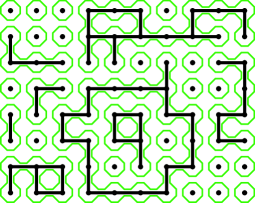
Figure 1: Example of an FK bond configuration in a rectangular region. Black dots represent vertices of $a{\mathbb{Z}}^{2}$, black horizontal and vertical edges represent FK bonds. The FK clusters are highlighted by lighter (green) loops on the medial lattice.

Using the FK representation, we can write the renormalized magnetization field $\Phi^{a}$ from Definition 1.1 as follows:

$$\Phi^{a}\stackrel{{\scriptstyle\mathrm{dist.}}}{{=}}\sum_{i}\sigma_{i}\mu_{C^{a}_{i}},$$ (5)

where $\mu_{C^{a}_{i}}:=\Theta_{a}\sum_{x\in C^{a}_{i}}\delta_{x}$ and the $\sigma_{i}$’s, as before, are $(\pm 1)$-valued, symmetric random variables independent of each other and everything else. We call the rescaled counting measure $\mu_{C^{a}_{i}}$ the area measure of the cluster $C^{a}_{i}$.

Roughly speaking, our first proof of uniqueness consists in showing that area measures have a scaling limit which is measurable with respect to the scaling limit of the collection of all macroscopic crossing events. (By crossing event we mean the occurrence of a path of FK bonds crossing a certain domain between two disjoint arcs on its boundary.)

To understand why this should be sufficient, let us associate in a unique way to each area measure $\mu_{C^{a}_{i}}$ the interface $\gamma^{a}_{i}$ in the medial lattice between the corresponding (rescaled) FK cluster $C^{a}_{i}$ and the surrounding FK clusters. Such interfaces form closed curves, or loops, which separate the corresponding clusters $C^{a}_{i}$ from infinity (see Figure 1). Announced results for FK percolation KemppainenSmirnovIII identify the scaling limit of those loops with $\mathrm{CLE}_{16/3}$, a random collection of nested loops which are locally distributed like $\mathrm{SLE}_{16/3}$ curves. The uniqueness of the collection of all macroscopic crossing events should then be a consequence of the results announced in KemppainenSmirnovIII (see Assumption 2.3 below and the discussion following it for more information).

The area measure of a cluster counts the number of vertices in that cluster. In particular, the sum of the area measures of clusters of diameter larger than some $\varepsilon$ counts the number of vertices from which a path of FK bonds of diameter larger than $\varepsilon$ originates. We call the occurrence of a path of FK bonds of diameter larger than $\varepsilon$ in the scaling limit a macroscopic one-arm event (see Section 2.2.3 for a precise definition of arm events), and we will sometimes call a one-arm vertex a vertex from which such a path originates. Since the area measures of macroscopic clusters count one-arm vertices, it is reasonable to expect that they be measurable with respect to the collection of all macroscopic crossing events. Indeed, the analogous result for Bernoulli percolation was proved in arXiv1008.1378 . Moreover, it is shown in MR2504956 that, in the scaling limit, only area measures corresponding to macroscopic clusters contribute to the magnetization, therefore the latter should also be measurable with respect to the collection of all macroscopic crossing events.

We end this section by briefly explaining the idea behind the proof that area measures are measurable with respect to the collection of macroscopic crossing events. Our proof of this fact will follow closely the proof of arXiv1008.1378 for Bernoulli percolation. This can be done because the main tools used in arXiv1008.1378 , such as FKG, RSW and certain bounds on the probability of arm events, are also available for Ising-FK percolation.

Although the proof is rather technical, the underlying idea is simple. Suppose we are interested in the Ising model on $a{\mathbb{Z}}^{2}\cap[0,1]^{2}$. We superimpose on $[0,1]^{2}$ a square grid with mesh $\varepsilon$, with $\varepsilon$ much smaller than 1 but much larger than $a$. We will show that the sum of the area measures of macroscopic FK clusters is well approximated by the number of squares of the $\varepsilon$-grid that intersect a macroscopic FK cluster, times the “mean” number of one-arm vertices inside a square of the $\varepsilon$-grid (we ignore all boundary issues in this discussion). This means that the number of one-arm vertices can be estimated by looking only at the macroscopic features of the FK configuration (i.e., at the collection of macroscopic crossing events).

Remark 2.1.

There are several advantages to the approach presented in this section. First, it shows that $\Phi^{\infty}$ is measurable with respect to the full scaling limit of FK-Ising percolation (plus a collection of random signs). Furthermore, it gives us a good way to visualize the magnetization in terms of area measures, as in (5).

Such a geometric representation as (5) would also be possible directly for the limiting magnetization field $\Phi^{\infty}$ if one could obtain the scaling limit of the collection of all individual, macroscopic area measures. This should be possible with methods similar to those used in this paper and in arXiv1008.1378 , and the resulting scaling limit should be expressible as a collection of orthogonal measures supported on “continuum FK clusters.”

We do not pursue this here since looking at the total number of $+$ and $-$ macroscopic one-arm vertices in a given domain is sufficient to prove the uniqueness of the limiting magnetization field, but we point out that approximating $\Phi^{\infty}$ using an a.s. finite number of signed measures could be useful if one wanted to determine the smallest $\varepsilon>0$ such that $\Phi^{\infty}$ is in the Sobolev space $\mathcal{H}^{-\varepsilon}$. The latter problem is briefly discussed in Remark A.4.

2.2 Setup for the proof of convergence

2.2.1 Notation, space of percolation configurations, compactness

Wewill work with the following setup: denote by $\sigma_{a}$ an Ising configuration on $a\mathbb{Z}^{2}\cap[0,1]^{2}$. As explained in Section 2.1, $\sigma_{a}$ can be obtained from an FK configuration $\omega_{a}$ on $a\mathbb{Z}^{2}\cap[0,1]^{2}$ by flipping an independent $\{\pm\}$ fair coin for each cluster of $\omega_{a}$. Let $\omega_{a}^{+}$ (resp., $\omega_{a}^{-}$) be the configuration consisting of the clusters of $\omega_{a}$ which have been chosen to be plus (resp., minus). Let us denote by $\bar{\omega}_{a}$ the coupled pair $(\omega_{a}^{+},\omega_{a}^{-})$. Note that one has $\omega_{a}=\omega_{a}^{+}\cup\omega_{a}^{-}$.

It will be very convenient to consider these FK configurations $\omega_{a}$ as (random) variables in a compact metrizable space $(\mathscr{H},\mathcal{T})=(\mathscr{H}_{[0,1]^{2}},\mathcal{T})$ which encodes all macroscopic crossing events. We say that an FK configuration $\omega_{a}$ contains a crossing of a domain $D$ between two disjoint arcs, $I_{1}$ and $I_{2}$, of its boundary $\partial D$ if there is a collection of edges from $\omega_{a}$ such that the edges form a connected set contained in $D$ except for two edges which intersect $I_{1}$ and $I_{2}$, respectively.

The compact space $(\mathscr{H},\mathcal{T})$ is not specific to our study of FK percolation and one can in fact rely here on the setup which was introduced by Schramm and Smirnov in SS in the case of independent percolation ($q=1$). Very briefly, it works as follows: the space of percolation configurations built in SS is the space of closed hereditary subsets of the space of quads $(\mathcal{Q},d_{\mathcal{Q}})$. Roughly speaking, this means that a point $\omega\in\mathscr{H}$ corresponds to a family of quads $Q\in\mathcal{Q}$ which is closed in $(\mathcal{Q},d_{\mathcal{Q}})$ and which satisfies the following constraint: if $Q\in\omega$ and $Q^{\prime}$ is “easier” to be traversed, then $Q^{\prime}$ is in $\omega$ as well. In SS, it is proved that this space $\mathscr{H}$ can be endowed with a topology $\mathcal{T}$ so that the topological space $(\mathscr{H},\mathcal{T})$ is compact, Hausdorff and metrizable. For convenience, we will choose a (nonexplicit) metric $d_{\mathscr{H}}$ on $\mathscr{H}$ which induces the topology $\mathcal{T}$. See SS for a clear exposition of the topological space $(\mathscr{H},\mathcal{T})$. See also arXiv1008.1378 , GPS2b .

Since we will need the crossing properties of the $+$ versus the $-$ clusters, we will in fact consider $\bar{\omega}_{a}=(\omega_{a}^{+},\omega_{a}^{-})$ as a random variable in the compact metrizable space $\mathscr{H}\times\mathscr{H}$ endowed with the product topology.

What is known about the limit as $a\to 0$ of the coupling $\bar{\omega}_{a}=(\omega_{a}^{+},\omega_{a}^{-})\in\mathscr{H}\times\mathscr{H}$? First of all, the tightness for $(\bar{\omega}_{a})_{a>0}$ follows immediately from the compactness of $(\mathscr{H}\times\mathscr{H},\mathcal{T}\otimes\mathcal{T})$.

Fact 2.2.

The random variable $\bar{\omega}_{a}=(\omega_{a}^{+},\omega_{a}^{-})$ is in $\mathscr{H}\times\mathscr{H}$ (with the product topology). Since $\mathscr{H}\times\mathscr{H}$ is compact for the product topology $\mathcal{T}\otimes\mathcal{T}$, there are subsequential scaling limits for $(\bar{\omega}_{a})_{a>0}$ as $a\to 0$.

Our goal will be to show that the scaling limit $\Phi^{\infty}$ of the magnetization field $\Phi^{a}$ is measurable with respect to the scaling limit of $\bar{\omega}_{a}$. This is the content of the main result of this section, Theorem 2.5. That theorem, together with Assumption 2.3 below, immediately implies the uniqueness of $\Phi^{\infty}$.

2.2.2 Scaling limit for $(\bar{\omega}_{a})_{a>0}$

It is known since the breakthrough paper MR2680496 that certain discrete “observables” for critical FK-percolation are asymptotically conformally invariant. These observables can then be used CDHKS to prove that interfaces have a scaling limit described by $\mathrm{SLE}_{16/3}$ curves. In our case, we need a full scaling limit result. Indeed, our later results in this section of the paper are based on the following hypothesis.

Assumption 2.3.

The coupled configurations $\bar{\omega}_{a}=(\omega_{a}^{+},\omega_{a}^{-})$ considered as random points in $(\mathscr{H}\times\mathscr{H},\mathcal{T}\otimes\mathcal{T})$ have a (unique) scaling limit as $a\searrow 0$; they converge in law to a continuum $\mathrm{FK}$ $\bar{\omega}_{\infty}=(\omega_{\infty}^{+},\omega_{\infty}^{-})$.

This assumption is very reasonable, based on the convergence of discrete interfaces to $\mathrm{SLE}_{16/3}$ curves CDHKS . An even clearer evidence is provided by the work in progress KemppainenSmirnovIII , where it is shown that the branching exploration tree converges to the branching $\mathrm{SLE}_{16/3}$ tree. However, as explained in SS, it is not always easy to go from one notion of scaling limit to another. In the case of Bernoulli percolation (i.e., the random-cluster model with $q=1$), the first and third author proved MR2249794 the existence and several properties of the full scaling limit as the collection of all cluster boundaries, building the limit object from $\mathrm{SLE}_{6}$ loops, and, as explained in arXiv1008.1378 , Section 2.3, their results imply convergence also in the “quad topology” $(\mathscr{H},\mathcal{T})$.

In our present case, the FK percolation analog of the result contained in MR2249794 , that is, the convergence of $\omega_{a}$ to $\mathrm{CLE}_{16/3}$, was announced in KemppainenSmirnovIII . From this convergence result, following arXiv1008.1378 , Section 2.3, and using Corollary 5.9 of DuminilSixArm instead of the analogous result for Bernoulli percolation, one should be able to obtain the convergence of $\omega_{a}$ to $\omega_{\infty}$ in the topological space $(\mathscr{H},\mathcal{T})$, exactly as in the case of Bernoulli percolation.

This step would justify the convergence of $\omega_{a}$ to $\omega_{\infty}$ in $(\mathscr{H},\mathcal{T})$, but we need slightly more, that is, the convergence of $\bar{\omega}_{a}$ to $\bar{\omega}_{\infty}$. However, note that the configurations $\omega_{a}^{+}$ and $\omega_{a}^{-}$ can be obtained from $\omega_{a}$ by tossing a fair coin for each cluster in $\omega_{a}$ to decide its sign. This suggests that the convergence of the configurations $\omega_{a}^{+}$ and $\omega_{a}^{-}$ should follow from the same arguments giving the convergence of $\omega_{a}$.

While the preceding discussion is clearly not a complete proof, it explains why Assumption 2.3 is very reasonable in the light of the announced results on the full scaling limit of FK percolation.

2.2.3 Measurable events in $\mathscr{H}\times\mathscr{H}$

In this subsection, we follow very closely Section 2.4. in arXiv1008.1378 . We refer to that paper for more details and will only highlight briefly how to adapt the definitions to our present case.

Let $A=(\partial_{1}A,\partial_{2}A)\subset[0,1]^{2}$ be a fixed topological annulus whose boundary, $\partial_{1}\cup\partial_{2}$ is composed of piecewise smooth cirves. We will often rely on the one-arm events $\mathcal{A}^{\pm}=\mathcal{A}_{1}^{\pm}$ which are in the Borel sigma field of $(\mathscr{H}\times\mathscr{H},\mathcal{T}\otimes\mathcal{T})$ and which are defined as follows:

$$\mathcal{A}_{1}^{+} := \bigl{\{}\bar{\omega}\in\mathscr{H}\times\mathscr{H},\exists Q\in\mathcal{Q}\mbox{ s.t. }Q\in\omega^{+}$$

$$\hskip 22.0pt\mbox{ and $Q$ connects }\partial_{1}A\mbox{ with }\partial_{2}A\bigr{\}}.$$

The event $\mathcal{A}_{1}^{-}$ is defined in the obvious related manner. We may also define the one-arm event $\mathcal{A}_{1}$ on the “uncolored” space $\mathscr{H}$. We will need the following extension of Lemma 2.4 in arXiv1008.1378 whose proof applies easily to our present case. The proof is analogous to that of Lemma 2.4 in arXiv1008.1378 , with the difference that Theorem 5.8 and Corollary 5.9 of DuminilSixArm replace the corresponding results for Bernoulli percolation used in arXiv1008.1378 .

Lemma 2.4 ((See Lemma 2.4 in arXiv1008.1378 )).

Let $A$ be a piecewise smooth annulus in $[0,1]^{2}$. Then

$$\mathbb{P}\bigl{[}\bar{\omega}_{a}\in\mathcal{A}_{1}^{\pm}\bigr{]}\longrightarrow\mathbb{P}\bigl{[}\bar{\omega}_{\infty}\in\mathcal{A}_{1}^{\pm}\bigr{]}$$

as the mesh size $a\to 0$. Furthermore, in any coupling of the measures $\mathbb{P}_{a}$ and $\mathbb{P}_{\infty}$ on the space $(\mathscr{H}\times\mathscr{H},\mathcal{T}\otimes\mathcal{T})$, in which $\bar{\omega}_{a}\to\bar{\omega}_{\infty}$ a.s. we have that $\mathbh{1}_{\mathcal{A}_{1}^{\pm}}(\bar{\omega}_{a})\to\mathbh{1}_{\mathcal{A}_{1}^{\pm}}(\bar{\omega}_{\infty})$ almost surely.

If $A$ is the annulus $[-c_{1},c_{1}]^{2}\setminus[-c_{2}/2,c_{2}/2]^{2}$, we define $\alpha_{1}^{\mathrm{FK}}(c_{2},c_{1})={\mathbb{P}[\omega_{\infty}^{+}\in\mathcal{A}_{1}]}$.

2.2.4 General setup of convergence: The space $\mathscr{H}\times\mathscr{H}\times\mathcal{H}^{-3}$

Let us consider the coupling $(\bar{\omega}_{a},\Phi^{a}(\bar{\omega}_{a}))=(\omega_{a}^{+},\omega_{a}^{-},\Phi^{a})\in\mathscr{H}\times\mathscr{H}\times\mathcal{H}^{-3}$. In order to prove our main Theorem 1.2, will prove the following stronger result.

Theorem 2.5 ((Under Assumption 2.3))

The random variables $(\bar{\omega}_{a},\Phi^{a})\in\mathscr{H}\times\mathscr{H}\times\mathcal{H}^{-3}$ converge in law as the mesh size $a\to 0$ to $(\bar{\omega}_{\infty},\Phi^{\infty})$ for the topology induced by the metric $d_{\mathscr{H}}\oplus d_{\mathscr{H}}\oplus\|\cdot\|_{\mathcal{H}^{-3}}$.

Furthermore, the limiting random variable $\Phi^{\infty}\in\mathcal{H}^{-3}$ is measurable with respect to $\bar{\omega}_{\infty}$, that is, we have

$$\Phi^{\infty}=\Phi^{\infty}(\bar{\omega}_{\infty}).$$

From Proposition A.2, we already know that $(\bar{\omega}_{a},\Phi^{a}(\bar{\omega}))$ is tight in the space $\mathscr{H}\times\mathscr{H}\times\mathcal{H}^{-3}$ endowed with the metric $d_{\mathscr{H}}\oplus d_{\mathscr{H}}\oplus\|\cdot\|_{\mathcal{H}^{-3}}$. As in Corollary 1.11, one thus has subsequential scaling limits: that is, one can find a subsequence $a_{k}\to 0$ such that $(\bar{\omega}_{a_{k}},\Phi^{a_{k}})$ converges in law to $(\bar{\omega}_{\infty},\Phi^{*})$ (here we use Assumption 2.3 which says that there is a unique possible subsequential scaling limit for $\bar{\omega}_{a}$). Since the space $(\mathscr{H}\times\mathscr{H}\times\mathcal{H}^{-3},d_{\mathscr{H}}\oplus d_{\mathscr{H}}\oplus\|\cdot\|_{\mathcal{H}^{-3}})$ is a complete separable metric space, one can apply Skorohod’s theorem. This gives us a joint coupling of the above processes such that

$$\bigl{(}\bar{\omega}_{a_{k}},\Phi^{a_{k}}\bigr{)}\stackrel{{\scriptstyle\mathrm{a.s.}}}{{\longrightarrow}}\bigl{(}\bar{\omega}_{\infty},\Phi^{*}\bigr{)}.$$ (7)

Proving Theorem 2.5 boils down to proving that $\Phi^{*}$ is in fact measurable with respect to $\bar{\omega}_{\infty}$. Achieving this would indeed conclude the proof of Theorem 2.5 (and thus Theorem 1.2) since it would uniquely characterize the subsequential scaling limits of $(\bar{\omega}_{a},\Phi^{a})$.

The purpose of the next subsection is to reduce the proof of Theorem 2.5 to the study of the renormalized magnetization in a square box.

2.2.5 Reduction to the renormalized magnetization in a dyadic box

We wish to prove Theorem 2.5, that is, to show that if $(\bar{\omega}_{a_{k}},\Phi^{a_{k}})\stackrel{{\scriptstyle\mathrm{a.s.}}}{{\longrightarrow}}(\bar{\omega}_{\infty},\Phi^{*})$, then $\Phi^{*}$ can be expressed as a measurable function of $\bar{\omega}_{\infty}$. Since $\Phi^{*}\in\mathcal{H}^{-3}$, it can be decomposed in the orthonormal basis $\{e_{j,k}\}_{j,k\geq 1}$, introduced in Appendix A, of the space $C^{\infty}_{0}([0,1]^{2})$ endowed with the $L^{2}$ norm: if $f=\sum_{j,k\geq 1}a_{j,k}e_{j,k}\in C^{\infty}_{0}([0,1]^{2})$, then

$$\bigl{\langle}\Phi^{*},f\bigr{\rangle}=\sum_{j,k\geq 1}\bigl{\langle}\Phi^{*},e_{j,k}\bigr{\rangle}a_{j,k},$$

which we write as

$$\Phi^{*}=\sum_{j,k\geq 1}\bigl{\langle}\Phi^{*},e_{j,k}\bigr{\rangle}e_{j,k}.$$ (8)

From the a.s. convergence (7), we have that for any fixed $j,k\geq 1$:

$$\bigl{(}\bar{\omega}_{a_{k}},\bigl{\langle}\Phi^{a_{k}},e_{j,k}\bigr{\rangle}\bigr{)}\stackrel{{\scriptstyle\mathrm{a.s.}}}{{\longrightarrow}}\bigl{(}\bar{\omega}_{\infty},\bigl{\langle}\Phi^{*},e_{j,k}\bigr{\rangle}\bigr{)},$$

where the convergence holds for the metric $d_{\mathscr{H}}\oplus d_{\mathscr{H}}\oplus\|\cdot\|_{\mathbb{R}}$. In order to prove Theorem 2.5, thanks to the decomposition (8), we only need to prove that for each fixed $j,k\geq 1$, the limiting quantity $\langle\Phi^{*},e_{j,k}\rangle$ is itself measurable w.r.t. $\bar{\omega}_{\infty}$.

It turns out that one can further reduce the difficulty of this task by approximating the functions $\{e_{j,k}\}_{j,k\geq 1}$ using step functions as follows. Let us fix some $j,k\geq 1$. For any small $\beta>0$, one can find dyadic squares $B_{i}$ and real numbers $b_{i}$ so that if $g_{\beta}:=\sum_{i}b_{i}1_{B_{i}}$, then

$$\|e_{j,k}-g_{\beta}\|_{L^{\infty}([0,1]^{2})}<\beta.$$

Now, exactly as in the proof of Lemma A.3, it is not hard to check that

$$\mathbb{E}\bigl{[}\bigl{(}\bigl{\langle}\Phi^{a},e_{j,k}\bigr{\rangle}-\bigl{\langle}\Phi^{a},g_{\beta}\bigr{\rangle}\bigr{)}^{2}\bigr{]}\leq C\beta^{2},$$

uniformly in $a>0$ (for some universal constant $C>0$). If one can show that, as $a_{k}\searrow 0$, $\langle\Phi^{a_{k}},g_{\beta}\rangle$ converges a.s. to a measurable function $G_{\beta}(\bar{\omega}_{\infty})$, then using the uniform $L^{2}$ bounds from Appendix A together with the triangle inequality in $L^{2}$, it follows that $G_{\beta}(\bar{\omega}_{\infty})$ converges as $\beta\to 0$ in $L^{2}$ to $\langle\Phi^{*},e_{j,k}\rangle$. Since $L^{2}$ is complete, $G_{\beta}(\bar{\omega}_{\infty})$ has an $L^{2}$-limit $G_{0}$ as $\beta\to 0$ which is itself measurable w.r.t. $\bar{\omega}_{\infty}$ and one has necessarily that $\langle\Phi^{*},e_{j,k}\rangle\stackrel{{\scriptstyle\mathrm{a.s.}}}{{=}}G_{0}(\bar{\omega}_{\infty})$. Since $G_{\beta}$ is a linear combination of magnetizations in dyadic squares, it follows from the above discussion that Theorem 2.5 is a corollary of the following theorem.

Theorem 2.6

Let $B$ be any dyadic square in $[0,1]^{2}$ and let the renormalized magnetization in $B$ be the random variable

$$m^{a}_{B}=m^{a}:=a^{15/8}\sum_{x\in a\mathbb{Z}^{2}\cap B}\sigma_{x}.$$

Then the coupled random variable $(\bar{\omega}_{a},m^{a})\in\mathscr{H}\times\mathscr{H}\times L^{2}$ converges in law as the mesh size $a\to 0$ to $(\bar{\omega}_{\infty},m)$ for the topology induced by the metric $d_{\mathscr{H}}\times d_{\mathscr{H}}\times\|\cdot\|_{L^{2}}$. Furthermore, the limiting random variable $m\in L^{2}$ is measurable with respect to $\bar{\omega}_{\infty}$, that is, we have

$$m=m(\bar{\omega}_{\infty}).$$

We now turn to the proof of this theorem. Without loss of generality and for the sake of simplicity, we may assume that our dyadic square $B$ is just $[0,1]^{2}$.

2.3 Scaling limit for the magnetization random variable (proof of Theorem 2.6)

2.3.1 Structure of the proof of Theorem 2.6

The setup for the scaling limit of $m^{a}$ is similar to the setup we explained above (in Section 2.2.4) for the scaling limit of $\Phi^{a}$. Namely, we consider the coupling $(\bar{\omega}_{a},m^{a})$ embedded in the metric space $(\mathscr{H}^{2}\times L^{2},d_{\mathscr{H}}\oplus d_{\mathscr{H}}\oplus\|\cdot\|_{L^{2}})$. The tightness of $(\bar{\omega}_{a},m^{a})$ easily follows from the stronger tightness of Proposition A.2 (see also MR2504956 and Camia ). In particular, there exist subsequential scaling limits

$$\bigl{(}\bar{\omega}_{a_{k}},m^{a_{k}}\bigr{)}\stackrel{{\scriptstyle d}}{{\longrightarrow}}\bigl{(}\bar{\omega}_{\infty}^{*},m^{*}\bigr{)}.$$

By Assumption 2.3, there is a unique possible law for $\bar{\omega}_{\infty}^{*}$, which we denoted by $\bar{\omega}_{\infty}$. In order to prove Theorem 2.6, it remains to show that the second coordinate $m^{*}\in L^{2}$ is measurable with respect to the first one.

As previously, let us couple all these random variables using Skorohod’s theorem so that

$$\bigl{(}\bar{\omega}_{a_{k}},m^{a_{k}}\bigr{)}\stackrel{{\scriptstyle\mathrm{a.s.}}}{{\longrightarrow}}\bigl{(}\bar{\omega}_{\infty},m^{*}\bigr{)}$$ (9)

for the metric $d_{\mathscr{H}}\oplus d_{\mathscr{H}}\oplus\|\cdot\|_{L^{2}}$.

The main idea will be to approximate the quantity $m^{a}$ by relying only on “macroscopic information” from the coupled configuration $\bar{\omega}_{a}$. The “macroscopic quantities” we are allowed to use are the quantities which are preserved in the scaling limit $\bar{\omega}_{a}\to\bar{\omega}_{\infty}$ (i.e., crossing events and so on, see Section 2.2.3).

We will approximate the magnetization $m^{a}$ by a two step procedure. Roughly speaking, we first approximate the magnetization as a rescaled sum of spin variables $\sigma_{x}$ such that $x$ is the starting point of a “macroscopic” FK path, and then approximate the latter sum by means of “macroscopic” quantities following arXiv1008.1378 , as explained below.

For the first step, we fix some small dyadic scale $\rho\in\{2^{-k},k\in\mathbb{N}\}$ and divide the square $[0,1]^{2}$ along the grid $\rho\mathbb{Z}^{2}$. Let $S_{\rho}$ be the set of $\rho$-squares thus obtained. For each $\rho$-square $Q\in S_{\rho}$, consider the annulus $A_{Q}:=3Q\setminus Q$ where we denote by $3Q$ the square of side-length $3\rho$ centered on $Q$. We will divide the clusters in the FK-configuration $\omega_{a}$ in two groups: the clusters which cross at least one annulus $A_{Q},Q\in S_{\rho}$ and the clusters which do not cross any annulus. We may rewrite the magnetization $m^{a}$ as follows:

$$m^{a} = \sum_{x\in[0,1]^{2}\cap a\mathbb{Z}^{2}}a^{15/8}\sigma_{x}$$ (10)

$$= \sum_{Q\in S_{\rho}}\biggl{(}\sum_{x\in Q\dvtx x\leftrightarrow\partial(3Q)}a^{15/8}\sigma_{x}+\sum_{x\in Q\dvtx x\nleftrightarrow\partial(3Q)}a^{15/8}\sigma_{x}\biggr{)}.$$ (11)

Following MR2504956 (with a slightly different setup here), let us show that the contribution of the second inside sum is negligible in $L^{2}$. Indeed,

$$\biggl{\|}\sum_{Q\in S_{\rho}}\sum_{x\in Q\dvtx x\nleftrightarrow\partial(3Q)}a^{15/8}\sigma_{x}\biggr{\|}_{2}^{2}$$

$$\qquad=\sum_{Q,Q^{\prime}}\sum_{x,y}a^{15/4}{\mathbb{E}[\sigma_{x}\sigma_{y}1_{x\in Q\dvtx x\nleftrightarrow\partial(3Q)}1_{y\in Q^{\prime}\dvtx y\nleftrightarrow\partial(3Q^{\prime})}]}$$

$$\qquad=\sum_{Q,Q^{\prime}}\sum_{x,y}a^{15/4}{\mathbb{E}[1_{x\leftrightarrow y}1_{x\in Q\dvtx x\nleftrightarrow\partial(3Q)}1_{y\in Q^{\prime}\dvtx y\nleftrightarrow\partial(3Q^{\prime})}]}$$ (12)

$$\qquad\leq\sum_{x,y\dvtx|x-y|\leq 8\rho}a^{15/4}{\mathbb{E}[1_{x\leftrightarrow y}]}$$ (13)

$$\qquad=a^{15/4}O\biggl{(}a^{-2}\biggl{(}\frac{8\rho}{a}\biggr{)}^{2}(\rho/a)^{-1/4}\biggr{)}$$ (14)

$$\qquad=O\bigl{(}\rho^{7/4}\bigr{)}.$$ (15)

Since we are looking for a limiting law for $m^{a}$ in $L^{2}$, it is thus enough [up to a small error of $O(\rho^{7/4})$] to focus on the first summand

$$m^{a}_{\rho}:=\sum_{Q\in S_{\rho}}\sum_{x\in Q\dvtx x\leftrightarrow\partial(3Q)}a^{15/8}\sigma_{x}.$$

Since $\rho>0$ is fixed and the mesh size $a\to 0$, we are getting closer to an approximation by “macroscopic quantities.” We still need to approximate in a suitable macroscopic manner the quantity

$$L_{Q}^{a}=L_{Q}^{a}(\bar{\omega}_{a}):=\sum_{x\in Q\dvtx x\leftrightarrow\partial(3Q)}a^{15/8}\sigma_{x}$$

for each $\rho$-square $Q\in S_{\rho}$. This is the second step of our approximation procedure and for this we will follow very closely the proof in arXiv1008.1378 of the scaling limit of counting measures on pivotal points (called pivotal measures). In the rest of the proof, let us fix the value of $\rho$ and fix some $\rho$-square $Q\in S_{\rho}$.

Let $\varepsilon>0$ be some small fixed threshold (such that $a\ll\varepsilon\ll\rho$). Divide the square $Q\cap a\mathbb{Z}^{2}$ into equal disjoint squares of side-length $\varepsilon_{a}:=a\lfloor{\varepsilon/a}\rfloor$. There are $N=\Omega(\varepsilon^{-2})$ such squares inside $Q$ (we do not need to keep the dependence in $\rho$ in what follows) plus $O(\varepsilon^{-1})$ squares which intersect the boundary of $Q$. Let $(B_{i})_{i\in\{1,\ldots,N\}}$ denote the set of such $\varepsilon_{a}$-squares inside $Q$.

For each $i\in[N]:=\{1,\ldots,N\}$, let

$$X_{i}^{\varepsilon}=X_{i}:=\sum_{x\in B_{i}\dvtx x\leftrightarrow\partial(3Q)}a^{15/8}\sigma_{x}.$$ (16)

Furthermore, let $B:=\cup B_{i}\subset Q$. We thus have

$$L_{Q}^{a}=\sum_{i\in[N]}X_{i}^{\varepsilon}+\sum_{x\in Q\setminus B\dvtx x\leftrightarrow\partial(3Q)}a^{15/8}\sigma_{x}.$$ (17)

The second term (which arises when $\rho$ is not a multiple of $\varepsilon_{a}$) turns out to be negligible in $L^{2}$ as well. Indeed,

$$\biggl{\|}\sum_{x\in Q\setminus B\dvtx x\leftrightarrow\partial(3Q)}a^{15/8}\sigma_{x}\biggr{\|}_{2}^{2} \leq \sum_{x,y\in Q\setminus B}a^{15/4}{\mathbb{P}[x\leftrightarrow y]}$$ (18)

$$\leq O(1)a^{15/4}\frac{\rho}{\varepsilon}\sum_{k=1}^{\rho/\varepsilon}\biggl{(}\frac{\varepsilon}{a}\biggr{)}^{4}\biggl{(}\frac{a}{k\varepsilon}\biggr{)}^{1/4}$$ (19)

$$\leq O(1)\frac{\rho}{\varepsilon}(\rho/\varepsilon)^{3/4}\varepsilon^{4}\varepsilon^{-1/4}$$ (20)

$$\leq O(1)\rho^{7/4}\varepsilon^{2}.$$ (21)

Therefore, as $\varepsilon$ goes to zero, and uniformly in the mesh size $a\leq\varepsilon$, the boundary term is negligible in $L^{2}$. It thus remains to control the term $\sum_{i\in[N]}X_{i}^{\varepsilon}$.

For this, let us introduce for each $i\in[N]$, the variables

$$Y_{i}^{\varepsilon}=Y_{i}^{\varepsilon}(\bar{\omega}_{a}):=1_{\{B_{i}\stackrel{{\scriptstyle\omega_{a}^{+}}}{{\longleftrightarrow}}\partial(3Q)\}}-1_{\{B_{i}\stackrel{{\scriptstyle\omega_{a}^{-}}}{{\longleftrightarrow}}\partial(3Q)\}}.$$ (22)

We will prove in the next subsection the following proposition.

Proposition 2.7.

There exists a universal constant $c>0$ such that for any square $Q$ of side-length $\rho$ as above, we have

$$\biggl{\|}\sum_{i\in[N]}X_{i}^{\varepsilon}-c\beta(\varepsilon)\sum_{i\in[N]}Y_{i}^{\varepsilon}\biggr{\|}_{2}\longrightarrow 0$$ (23)

as $\varepsilon\to 0$ uniformly in $a\leq\varepsilon$ and where $\beta(\varepsilon):=\varepsilon^{2}\alpha_{1}^{\mathrm{FK}}(\varepsilon,1)^{-1}$ and $\alpha_{1}^{\mathrm{FK}}(\varepsilon,1)$ is the probability of the one-arm event in the annulus $[-1,1]^{2}\setminus[-\varepsilon/2,\varepsilon/2]^{2}$ for $\omega_{\infty}^{+}$.

Before proving the proposition, let us explain why it indeed implies Theorem 2.6. From Section 2.2.3, it follows that the functions $Y_{i}^{\varepsilon}$ defined in (22) can be seen as measurable functions of $\bar{\omega}_{\infty}$ and that, for each $i\in[N]$, along the above subsequence $(a_{k})$, one has [see equation (9)]:

$$Y_{i}^{\varepsilon}(\bar{\omega}_{a_{k}})\stackrel{{\scriptstyle\mathrm{a.s.}}}{{\longrightarrow}}Y_{i}^{\varepsilon}(\bar{\omega}_{\infty}).$$

Furthermore, one can see from Proposition 2.7 that $\|\beta(\varepsilon)\sum Y_{i}^{\varepsilon}(\bar{\omega}_{a})\|_{2}$ is bounded uniformly in $0<a\leq\varepsilon$. This implies, modulo some triangle inequalities, that

$$\Bigl{\|}L_{Q}^{a}(\bar{\omega}_{a_{k}})-c\beta(\varepsilon)\sum Y_{i}^{\varepsilon}(\bar{\omega}_{\infty})\Bigr{\|}_{2}\longrightarrow 0,$$

uniformly in $0<a_{k}<\varepsilon$. This in turn implies that the sequence $(c\beta(\varepsilon)\times\break\sum Y_{i}^{\varepsilon}(\bar{\omega}_{\infty}))_{\varepsilon>0}$ is a Cauchy-sequence in $L^{2}$. In particular, it has an $L^{2}$-limit that we may denote by $L_{Q}(\bar{\omega}_{\infty})$ and this $L^{2}$-limit is such that

$$\bigl{\|}L_{Q}^{a_{k}}(\bar{\omega}_{a_{k}})-L_{Q}(\bar{\omega}_{\infty})\bigr{\|}_{2}\longrightarrow 0$$

as the mesh size $a_{k}\to 0$.

Using the above estimates, we have that

$$\biggl{\|}m^{a_{k}}-\sum_{Q}L_{Q}(\bar{\omega}_{\infty})\biggr{\|}_{2}^{2}\longrightarrow 0,$$

uniformly in $0<a_{k}<\rho$. Exactly as above with the second order approximation in $\varepsilon$, the above displayed equation (plus the $L^{2}$ bounds we already have) implies that the Cauchy sequence $(\sum_{Q}L_{Q}(\bar{\omega}_{\infty}))_{\rho>0}$ has an $L^{2}$-limit denoted by $m(\bar{\omega}_{\infty})$ as $\rho\to 0$. Finally, thanks to the a.s. convergence in equation (9), this $L^{2}$-limit must be such that

$$m^{*}\stackrel{{\scriptstyle\mathrm{a.s.}}}{{=}}m(\bar{\omega}_{\infty}),$$ (24)

which completes the proof of Theorem 2.6, modulo proving Proposition 2.7.

2.3.2 Proof of Proposition 2.7

We want to show that for any $\delta>0$, one can take $\varepsilon>0$ sufficiently small so that for any $0<a<\varepsilon<\rho$,

$$\mathbb{E}\Bigl{[}\Bigl{(}\sum X_{i}^{\varepsilon}-c\beta(\varepsilon)\sum Y_{i}^{\varepsilon}\Bigr{)}^{2}\Bigr{]}\leq\delta.$$

Let us decompose this quantity as follows.

$$\mathbb{E}\Bigl{[}\Bigl{(}\sum X_{i}^{\varepsilon}-c\beta(\varepsilon)\sum Y_{i}^{\varepsilon}\Bigr{)}^{2}\Bigr{]}$$

$$\qquad=\sum_{i,j}\mathbb{E}\bigl{[}\bigl{(}X_{i}^{\varepsilon}-c\beta(\varepsilon)Y_{i}^{\varepsilon}\bigr{)}\bigl{(}X_{j}^{\varepsilon}-c\beta(\varepsilon)Y_{j}^{\varepsilon}\bigr{)}\bigr{]}$$

(25)

$$\qquad\leq\sum_{i,j\dvtx d(B_{i},B_{j})\leq r}\bigl{(}\mathbb{E}\bigl{[}X_{i}^{\varepsilon}X_{j}^{\varepsilon}\bigr{]}+c^{2}\beta(\varepsilon)^{2}\mathbb{E}\bigl{[}Y_{i}^{\varepsilon}Y_{j}^{\varepsilon}\bigr{]}\bigr{)}$$

$$\quad\qquad{}+\sum_{i,j\dvtx d(B_{i},B_{j})>r}\mathbb{E}\bigl{[}\bigl{(}X_{i}^{\varepsilon}-c\beta(\varepsilon)Y_{i}^{\varepsilon}\bigr{)}\bigl{(}X_{j}^{\varepsilon}-c\beta(\varepsilon)Y_{j}^{\varepsilon}\bigr{)}\bigr{]},$$

where $r$ is a mesoscopic scale $\varepsilon\ll r\ll\rho$ which will be chosen later. To go from the first to the second line, we used that fact that the cross product terms are necessarily negative as can be seen by first conditioning on the noncolored FK configuration $\omega_{a}$.

The first term of the RHS of the above displayed inequality is easy to bound. Indeed,

$$\sum_{i,j\dvtx d(B_{i},B_{j})\leq r}\mathbb{E}\bigl{[}X_{i}^{\varepsilon}X_{j}^{\varepsilon}\bigr{]} \leq \sum_{x,y\in a\mathbb{Z}^{2}\cap Q\ \mathrm{s.t.}\ d(x,y)\leq 2r}a^{15/4}{\mathbb{E}[\sigma_{x}\sigma_{y}]}\leq O\bigl{(}r^{7/4}\bigr{)}$$

and similarly for $\sum_{i,j\dvtx d(B_{i},B_{j})\leq r}c^{2}\beta(\varepsilon)^{2}{\mathbb{E}[Y_{i}^{\varepsilon}Y_{j}^{\varepsilon}]}$. One can thus fix $r>0$ small enough so that, uniformly in $a<\varepsilon<r$, the first term in the RHS of (2.3.2) is $<\delta/2$.

For the second term, we proceed as in arXiv1008.1378 using a coupling argument. Proposition 2.7 will follow from the next lemma.

Lemma 2.8.

For any fixed $r<\rho<1$ and any $\tilde{\delta}>0$, one can choose $\varepsilon=\varepsilon(r,\rho,\tilde{\delta})>0$ small enough such that for any pair of squares $B_{i},B_{j}$ with $d(B_{i},B_{j})>r$, one has

$$\mathbb{E}\bigl{[}\bigl{(}X_{i}^{\varepsilon}-c\beta(\varepsilon)Y_{i}^{\varepsilon}\bigr{)}\bigl{(}X_{j}^{\varepsilon}-c\beta(\varepsilon)Y_{j}^{\varepsilon}\bigr{)}\bigr{]}\leq\frac{\tilde{\delta}}{2}\mathbb{E}\bigl{[}X_{i}^{\varepsilon}X_{j}^{\varepsilon}\bigr{]}.$$

Let us explain why this lemma is enough to conclude the proof. Summing the estimate provided by the lemma over all $B_{i},B_{j}$ with $d(B_{i},B_{j})>r$, one gets

$$\sum_{i,j\dvtx d(B_{i},B_{j})>r}\mathbb{E}\bigl{[}\bigl{(}X_{i}^{\varepsilon}-c\beta(\varepsilon)Y_{i}^{\varepsilon}\bigr{)}\bigl{(}X_{j}^{\varepsilon}-c\beta(\varepsilon)Y_{j}^{\varepsilon}\bigr{)}\bigr{]} \leq \frac{\tilde{\delta}}{2}\mathbb{E}\bigl{[}\bigl{(}L_{Q}^{a}(\bar{\omega}_{a})\bigr{)}^{2}\bigr{]}.$$

Now, it is straightforward to check that the second moment ${\mathbb{E}[(L_{Q}^{a}(\bar{\omega}_{a}))^{2}]}$ is bounded by $C\rho^{15/4}$ uniformly in $a<\varepsilon<\rho$ where $C$ is some universal constant. By choosing $\tilde{\delta}=\delta/C$, we conclude the proof.

Proof of Lemma 2.8 Let us fix two squares $B_{i}$ and $B_{j}$ at distance at least $r$ from each other. Conditioned on the event that both $B_{i}$ and $B_{j}$ are connected to $\partial(3Q)$, our strategy is to compare how things look within the $\varepsilon$-square $B_{i}$ with the following “test case.” Consider the $\varepsilon$-square $B_{0}$ centered at the origin and let $Q_{0}$ be the square $[-\rho,\rho]^{2}$ also centered at the origin. Let us define

$$X_{0}:=a^{15/8}\sum_{x\in a\mathbb{Z}^{2}\cap B_{0}}\sigma_{x}1_{\{x\leftrightarrow\partial Q_{0}\ \mathrm{in}\ \bar{\omega}_{a}\}}.$$ (26)

Recall the events $\mathcal{A}_{1}^{\pm}$ defined in Section 2.2.3 and applied here to the annulus $A=Q_{0}\setminus B_{0}$. We first wish to show that there is a constant $c>0$ such that

$$\cases{\mathbb{E}\bigl{[}X_{0}|{\mathcal{A}}_{1}^{+}\bigr{]}\sim c\beta(\varepsilon),\vspace*{3pt}\cr\mathbb{E}\bigl{[}X_{0}|{\mathcal{A}}_{1}^{-}\bigr{]}\sim-c\beta(\varepsilon)}$$ (27)

uniformly as $0<a<\varepsilon$ go to 0. To see why this holds we note that, as in Section 4.5 in arXiv1008.1378 , one has that

$$\mathbb{E}\bigl{[}X_{0}|{\mathcal{A}}_{1}^{+}\bigr{]}\sim(\varepsilon/a)^{2}a^{15/8}\frac{\alpha_{1}^{\mathrm{FK}}(a,1)}{\alpha_{1}^{\mathrm{FK}}(\varepsilon,1)}.$$

To adapt the proof from arXiv1008.1378 , it is enough to have bounds on the half-plane exponents of critical FK percolation “in the bulk.” Such bounds follow from standard percolation arguments, using the RSW theorem of arXiv0912.4253 .

Now, using Theorem 1.3 (with $k=0$) in arXiv1202.2838 together with Wu’s result, Theorem 1.4, we have that $\alpha_{1}^{\mathrm{FK}}(a,1)\sim ca^{1/8}$ as $a\to 0$, which explains the desired asymptotic.

In what follows, for any $u\geq\varepsilon$, we will denote by $D_{u}$ ($\widetilde{D}_{u}$) the square centered around $B_{i}$ ($B_{j}$) of side-length $u$. Let us fix yet another mesoscopic scale $\gamma$ so that $\varepsilon\ll\gamma\ll r$ (e.g., $\gamma:=r^{2}$). Let $m:=d(B_{i},B_{j})/2$ and let $z$ be the midpoint between the centers of $B_{i}$ and $B_{j}$. Let $R^{+}$ be the event that $\{\partial D_{\gamma}\stackrel{{\scriptstyle\omega^{+}}}{{\longleftrightarrow}}\partial D_{m}\}\cap\{\mbox{there is a circuit of }\omega^{+}\mbox{ inside }D_{r}\setminus D_{\gamma}\mbox{ that surrounds }D_{\gamma}\}$ (see Figure 2). The event $R^{-}$ is defined similarly. Notice that $R^{+}\cap R^{-}=\varnothing$. On the event $R^{\pm}$, let $C=C(\bar{\omega})$ be the outermost such open circuit for the FK configuration $\omega\in\mathscr{H}$ (the outermost open circuit necessarily has the appropriate color).

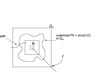
Figure 2: The event $R^{+}$.

Let us analyze in the term ${\mathbb{E}[(X_{i}-c\beta(\varepsilon)Y_{i}^{\varepsilon})(X_{j}-c\beta(\varepsilon)Y_{j}^{\varepsilon})]}$ the contribution coming from the event $(R^{+}\cup R^{-})^{c}$, namely,

$$\mathbb{E}\bigl{[}\bigl{(}X_{i}-c\beta(\varepsilon)Y_{i}^{\varepsilon}\bigr{)}\bigl{(}X_{j}-c\beta(\varepsilon)Y_{j}^{\varepsilon}\bigr{)};\bigl{(}R^{+}\cup R^{-}\bigr{)}^{c}\bigr{]}$$

$$\qquad\leq\mathbb{E}\bigl{[}X_{i}X_{j}+c^{2}\beta(\varepsilon)^{2}Y_{i}Y_{j};\bigl{(}R^{+}\cup R^{-}\bigr{)}^{c}\bigr{]}.$$

See the explanation after (2.3.2) as to why the cross product terms are negative. Following arXiv1008.1378 ,

$$\mathbb{E}\bigl{[}X_{i}X_{j};\bigl{(}R^{+}\cup R^{-}\bigr{)}^{c}\bigr{]}$$

$$\qquad=\mathbb{E}\bigl{[}X_{i}X_{j};\partial D_{\varepsilon}\stackrel{{\scriptstyle\omega}}{{\longleftrightarrow}}\partial D_{m};$$

$$\hskip 44.0pt\partial\widetilde{D}_{\varepsilon}\stackrel{{\scriptstyle\omega}}{{\longleftrightarrow}}\partial\widetilde{D}_{m};\partial B(z,2m)\stackrel{{\scriptstyle\omega}}{{\longleftrightarrow}}\partial(3Q);\bigl{(}R^{+}\cup R^{-}\bigr{)}^{c}\bigr{]}$$

$$\qquad\leq O(1){\mathbb{E}^{\mathrm{wired}}[\widetilde{X}_{i}]}{\mathbb{E}^{\mathrm{wired}}[\widetilde{X}_{j}]}\alpha_{1}^{\mathrm{wired}}(\varepsilon,\rho)\alpha_{1}^{\mathrm{wired}}(\varepsilon,\gamma)$$

$$\quad\qquad{}\times\mathbb{P}\bigl{[}\partial D_{\gamma}\stackrel{{\scriptstyle\omega}}{{\longleftrightarrow}}\partial D_{m};\bigl{(}R^{+}\cup R^{-}\bigr{)}^{c}\bigr{]},$$

where we have just used FKG and where we dominated $X_{i}$ by $\widetilde{X}_{i}$, the number of points in $B_{i}$ connected to $\partial B_{i}$ (we also used some straightforward quasi-multiplicativity for the one-arm FK event which follows easily from the RSW theorem in arXiv0912.4253 ; see, e.g., MR2523462 for an explanation of quasi-multiplicativity in the case of standard percolation and see DuminilSixArm for quasi-multiplicativity results in the case of FK percolation). Now, using FKG with RSW from arXiv0912.4253 , we get that there exists an exponent $\xi>0$ such that ${\mathbb{P}[R^{+}\cup R^{-}|\partial D_{\gamma}\stackrel{{\scriptstyle\omega}}{{\longleftrightarrow}}\partial D_{m}]}\geq 1-(\gamma/m)^{\xi}$, which implies that

$$\mathbb{P}\bigl{[}\partial D_{\gamma}\stackrel{{\scriptstyle\omega}}{{\longleftrightarrow}}\partial D_{m};\bigl{(}R^{+}\cup R^{-}\bigr{)}^{c}\bigr{]}\leq\alpha_{1}^{\mathrm{FK}}(\gamma,m)(\gamma/m)^{\xi}.$$

Altogether, we obtain that

$$\mathbb{E}\bigl{[}X_{i}X_{j};\bigl{(}R^{+}\cup R^{-}\bigr{)}^{c}\bigr{]}\leq O(1){\mathbb{E}[X_{i}X_{j}]}(\gamma/m)^{\xi}.$$

The term ${\mathbb{E}[c^{2}\beta(\varepsilon)^{2}Y_{i}Y_{j};(R^{+}\cup R^{-})^{c}]}$ can be treated similarly. We may thus focus our analysis on what is happening on the event $R^{+}\cup R^{-}$. Let $\mathcal{F}_{C}$ be the filtration induced by the configuration outside the contour $C$. One can write

$$\bigl{|}\mathbb{E}\bigl{[}\bigl{(}X_{i}-c\beta(\varepsilon)Y_{i}^{\varepsilon}\bigr{)}\bigl{(}X_{j}-c\beta(\varepsilon)Y_{j}^{\varepsilon}\bigr{)};R^{+}\cup R^{-}\bigr{]}\bigr{|}$$

$$\qquad=\mathbb{E}\bigl{[}\bigl{|}X_{j}-c\beta(\varepsilon)Y_{j}\bigr{|}\mathbb{E}\bigl{[}\bigl{|}X_{i}-c\beta(\varepsilon)Y_{i}\bigr{|}|\mathcal{F}_{C}\bigr{]};R^{+}\cup R^{-}\bigr{]},$$

since on the event $R^{+}\cup R^{-}$, the variable $|X_{j}-c\beta(\varepsilon)Y_{j}|$ is measurable w.r.t. $\mathcal{F}_{C}$. Now,

$$\mathbb{E}\bigl{[}\bigl{|}X_{j}-c\beta(\varepsilon)Y_{j}\bigr{|}\mathbb{E}\bigl{[}\bigl{|}X_{i}-c\beta(\varepsilon)Y_{i}\bigr{|}|\mathcal{F}_{C}\bigr{]};R^{+}\cup R^{-}\bigr{]}$$

$$\qquad=\mathbb{P}\bigl{[}R^{+}\bigr{]}\mathbb{E}\bigl{[}\bigl{|}X_{j}-c\beta(\varepsilon)Y_{j}\bigr{|}\mathbb{E}\bigl{[}\bigl{|}X_{i}-c\beta(\varepsilon)Y_{i}\bigr{|}|\mathcal{F}_{C}\bigr{]}|R^{+}\bigr{]}$$

$$\quad\qquad{}+\mathbb{P}\bigl{[}R^{-}\bigr{]}\mathbb{E}\bigl{[}\bigl{|}X_{j}-c\beta(\varepsilon)Y_{j}\bigr{|}\mathbb{E}\bigl{[}\bigl{|}X_{i}-c\beta(\varepsilon)Y_{i}\bigr{|}|\mathcal{F}_{C}\bigr{]}|R^{-}\bigr{]}.$$

Let us analyze the first term, it gives

$$\mathbb{P}\bigl{[}R^{+}\bigr{]}\mathbb{E}\bigl{[}\bigl{|}X_{j}-c\beta(\varepsilon)Y_{j}\bigr{|}\mathbb{E}\bigl{[}\bigl{|}X_{i}-c\beta(\varepsilon)Y_{i}\bigr{|}|\mathcal{F}_{C},R^{+}\bigr{]}|R^{+}\bigr{]}$$

$$\qquad=\mathbb{P}\bigl{[}R^{+}\bigr{]}\mathbb{E}\bigl{[}\bigl{|}X_{j}-c\beta(\varepsilon)Y_{j}\bigr{|}\mathbh{1}_{C\leftrightarrow\partial(3Q)}\mathbb{E}\bigl{[}\bigl{|}X_{i}-c\beta(\varepsilon)Y_{i}\bigr{|}|C,R^{+}\bigr{]}|R^{+}\bigr{]}$$

$$\qquad=\mathbb{P}\bigl{[}R^{+}\bigr{]}\mathbb{E}\bigl{[}\bigl{|}X_{j}-c\beta(\varepsilon)Y_{j}\bigr{|}\mathbh{1}_{C\leftrightarrow\partial(3Q)}\mathbb{P}\bigl{[}\partial B_{i}\leftrightarrow C|C,R^{+}\bigr{]}$$

$$\hskip 103.0pt{}\times\mathbb{E}\bigl{[}\bigl{|}X_{i}-c\beta(\varepsilon)Y_{i}\bigr{|}|C,\partial B_{i}\leftrightarrow C\bigr{]}|R^{+}\bigr{]}.$$

We will prove below the following lemma.

Lemma 2.9 ((Coupling lemma)).

For any contour $C$, we have the following control on the conditional expectation:

$$\mathbb{E}\bigl{[}\bigl{|}X_{i}-c\beta(\varepsilon)Y_{i}\bigr{|}|C,\partial B_{i}\leftrightarrow C\bigr{]}\leq K(\varepsilon/\gamma)^{\alpha}\beta(\varepsilon)$$

for some exponent $\alpha>0$ and some constant $K\in(0,\infty)$.

Plugging this lemma into the last displayed equation leads to

$$\mathbb{P}\bigl{[}R^{+}\bigr{]}\mathbb{E}\bigl{[}\bigl{|}X_{j}-c\beta(\varepsilon)Y_{j}\bigr{|}\mathbb{E}\bigl{[}\bigl{|}X_{i}-c\beta(\varepsilon)Y_{i}\bigr{|}|\mathcal{F}_{C},R^{+}\bigr{]}|R^{+}\bigr{]}$$

$$\qquad\leq C(\varepsilon/\gamma)^{\alpha}\beta(\varepsilon)\mathbb{P}\bigl{[}R^{+}\bigr{]}$$

$$\quad\qquad{}\times\mathbb{E}\bigl{[}\bigl{|}X_{j}-c\beta(\varepsilon)Y_{j}\bigr{|}\mathbh{1}_{C\leftrightarrow\partial 3Q}\mathbb{P}\bigl{[}\partial B_{i}\leftrightarrow C|C,R^{+}\bigr{]}|R^{+}\bigr{]}$$ (28)

$$\qquad\leq O(1)(\varepsilon/\gamma)^{\alpha}\beta(\varepsilon)\alpha_{1}^{\mathrm{FK}}(\gamma,m)$$

$$\quad\qquad{}\times\mathbb{E}\bigl{[}\bigl{|}X_{j}-c\beta(\varepsilon)Y_{j}\bigr{|}\mathbh{1}_{C\leftrightarrow\partial(3Q)}\mathbb{P}\bigl{[}\partial B_{i}\leftrightarrow C|C,R^{+}\bigr{]}|R^{+}\bigr{]}.$$

Now, similarly to the above analysis of what happens on the event $(R^{+}\cup R^{-})^{c}$, it is not hard to check by cutting into different scales and dominating by wired boundary conditions that

$$\mathbb{E}\bigl{[}\bigl{|}X_{j}-c\beta(\varepsilon)Y_{j}\bigr{|}\mathbh{1}_{C\leftrightarrow\partial(3Q)}\mathbb{P}\bigl{[}\partial B_{i}\leftrightarrow C|C,R^{+}\bigr{]}|R^{+}\bigr{]}$$

$$\qquad\leq O(1)\beta(\varepsilon)\alpha_{1}^{\mathrm{FK}}(\varepsilon,\rho)\alpha_{1}^{\mathrm{FK}}(\varepsilon,\gamma),$$

which together with (2.3.2) and quasi-multiplicativity gives us (since one has also the same estimate on the event $R^{-}$),

$$\bigl{|}\mathbb{E}\bigl{[}\bigl{(}X_{i}-c\beta(\varepsilon)Y_{i}^{\varepsilon}\bigr{)}\bigl{(}X_{j}-c\beta(\varepsilon)Y_{j}^{\varepsilon}\bigr{)};R^{+}\cup R^{-}\bigr{]}\bigr{|}$$

$$\qquad\leq O(1)(\varepsilon/\gamma)^{\alpha}\beta(\varepsilon)^{2}\frac{\alpha_{1}^{\mathrm{FK}}(\varepsilon,\rho)^{2}}{\alpha_{1}^{\mathrm{FK}}(m,\rho)}$$

$$\qquad\leq O(1)(\varepsilon/\gamma)^{\alpha}{\mathbb{E}[X_{i}X_{j}]},$$

which (modulo proving Lemma 2.9) completes our proof of Lemma 2.8.

2.3.3 Proof of Lemma 2.9

Let $\nu_{C}$ be the wired FK probability measure conditioned on $\partial B_{i}\leftrightarrow C$ and let $\nu_{0}$ be the FK probability measure in $Q_{0}$ conditioned on the event $\mathcal{A}_{1}=\mathcal{A}_{1}(\tilde{x}+Q_{0}\setminus B_{0})$, where we translated the annulus $A=Q_{0}\setminus B_{0}$ so that it surrounds $B_{i}$. Clearly, in the domain $\mathcal{D}_{C}$ (inside the circuit $C$), the measure $\nu_{C}$ dominates $\nu_{0}$. Using RSW from arXiv0912.4253 , there is an open circuit in $\mathcal{D}_{C}\setminus B_{i}$ for $\omega^{0}_{a}\sim\nu_{0}$ with $\nu_{0}$-probability at least $1-c(\varepsilon/\gamma)^{\xi}$. Let us call this event $W$. On the event $W$, let $\widetilde{C}$ be the outermost circuit inside $\mathcal{D}_{C}$ for $\omega_{a}^{0}$. Since $\nu_{C}$ dominates $\nu_{0}$, one can couple $\omega^{C}_{a}\sim\nu_{C}$ with $\omega^{0}_{a}$ so that on the event $W$, they share the same open circuit $\widetilde{C}$ and are conditioned inside $\mathcal{D}_{\widetilde{C}}$ only on the constraint $\{\partial B_{i}\leftrightarrow\widetilde{C}\}$; in particular, on the event $W$, in this coupling one has $X_{i}=X_{0}$. In order to prove Lemma 2.9, it is enough to show that ${\mathbb{E}[X_{i};W^{c}|C,\partial B_{i}\leftrightarrow C]}$ and ${\mathbb{E}[X_{0};W^{c}|C,\partial B_{i}\leftrightarrow C]}$ are negligible w.r.t. $\beta(\varepsilon)$, which is straightforward using the quantity ${\mathbb{E}[\widetilde{X}_{i}]}\times{\mathbb{P}[W^{c}]}$ as we did previously while analyzing what happened on the event $(R^{+}\cup R^{-})^{c}$.

3 Second proof of the scaling limit of $\Phi^{a}$ using the $n$-point functions of Chelkak, Hongler and Izyurov

In this part, we will give a different proof of Theorem 1.2, using the recent breakthrough results of Chelkak, Hongler and Izyurov in arXiv1202.2838 . From our tightness result obtained in Appendix A, recall that there exist subsequential scaling limits $\Phi^{\star}=\lim\Phi^{a_{n}}$ for the convergence in law in the space $\mathcal{H}^{-3}$. We wish to prove that there is a unique such subsequential scaling limit. For this, we will use the following classical fact (see, e.g., MR2814399 ).

Proposition 3.1.

If $h$ is a random distribution in $\mathcal{H}^{-3}$ (for the sigma-field generated by the topology of $\|\cdot\|_{\mathcal{H}^{-3}}$), then the law of $h$ is uniquely characterized by

$$\phi_{h}(f):=\mathbb{E}\bigl{[}e^{i\langle h,f\rangle}\bigr{]}$$

as a function of $f\in\mathcal{H}^{3}$.

Using the tightness property proved in Appendix A, Theorem 1.2 will thus follow from the next result.

Proposition 3.2.

For any $f\in\mathcal{H}^{3}$, the quantity

$$\phi_{\Phi^{a}}(f)=\mathbb{E}\bigl{[}e^{i\langle\Phi^{a},f\rangle}\bigr{]}$$

converges as the mesh size $a\searrow 0$.

The proof of this proposition will be divided into two main steps as follows:

1. [1.]

2. First, we will show that $\Phi^{a}$ has “uniform exponential moments” which will allow us to express its characteristic function using

   $$\phi_{\Phi^{a}}(f)=\mathbb{E}\bigl{[}e^{i\langle\Phi^{a},f\rangle}\bigr{]}=1+\sum_{k\geq 1}\frac{i^{k}{\mathbb{E}[\langle\Phi^{a},f\rangle^{k}]}}{k!}.$$

3. Then it remains to compute each $k$th moment ${\mathbb{E}[\langle\Phi^{a},f\rangle^{k}]}$, that is, to show uniqueness as $a\to 0$. For this, one uses the scaling limit results from arXiv1202.2838 together with Proposition 3.9 below which takes care of $k$-tuples of points in the plane where at least two points are close to each other.

Let us now state the main result we will use from arXiv1202.2838 .

Theorem 3.3 ((arXiv1202.2838 , Theorem 1.3))

Let $\Omega$ be a bounded simply connected domain, and $\Omega_{a}$ be discretizations of $\Omega$ (built from $\Omega\cap a\mathbb{Z}^{2}$). We denote by $\xi$ the boundary conditions chosen on $\Omega$, and we assume $\xi$ to be either $+$ or $\mathrm{free}$ here. Then, for any $k\geq 1$, there exist $k$-point functions

$$z_{1},\ldots,z_{k}\in\Omega^{k}\mapsto\langle\sigma_{z_{1}},\ldots,\sigma_{z_{k}}\rangle_{\Omega}^{\xi},$$

so that for any $\varepsilon>0$, as the mesh size $a\to 0$ and uniformly over all $z_{1},\ldots,z_{k}\in\Omega$ at distance at least $\varepsilon$ from $\partial\Omega$ and from each other, one has

$$\varrho(a)^{-k/2}\cdot{\mathbb{E}_{\Omega_{a}}^{\xi}[\sigma_{z_{1}},\ldots,\sigma_{z_{k}}]}\longrightarrow\langle\sigma_{z_{1}},\ldots,\sigma_{z_{k}}\rangle_{\Omega}^{\xi}.$$ (29)

[Recall that $\varrho(a)$ is the renormalization factor defined in (1).]

Furthermore, the functions $\langle\sigma_{z_{1}},\ldots,\sigma_{z_{k}}\rangle_{\Omega}^{\xi}$ are conformally covariant in the following sense: if $\phi\dvtx\Omega\to\Omega^{\prime}$ is a conformal map, then

$$\langle\sigma_{z_{1}},\ldots,\sigma_{z_{k}}\rangle_{\Omega}^{\xi}=\langle\sigma_{\phi(z_{1})},\ldots,\sigma_{\phi(z_{k})}\rangle_{\Omega^{\prime}}^{\xi}\prod\bigl{|}\phi^{\prime}(z_{i})\bigr{|}^{1/8}.$$

Remark 3.4.

• It is noted in arXiv1202.2838 that although their Theorem 1.3 is stated only for plus boundary conditions, the conclusions are valid for free and other boundary conditions as well.

• In arXiv1202.2838 , the discretization is slightly different, which means that our $k$-point function $\langle\sigma_{z_{1}},\ldots,\sigma_{z_{k}}\rangle_{\Omega}^{\xi}$ is equal to the one of arXiv1202.2838 only up to a constant factor.

• In most of this paper, we assume Wu’s result, Theorem 1.4. In particular, one can then use the above theorem with $a^{k/8}$ instead of $\varrho(a)^{k/2}$ (and with yet a further change of the $k$ point function by another scalar). See Section 4 for the analysis when one does not wish to assume Wu’s result.

3.1 Exponential moments for the magnetization random variable

In this section, we shall show that if $m^{a}$ denotes the magnetization random variable $\langle\Phi^{a},1_{[0,1]^{2}}\rangle$ (for wired or free boundary conditions on the square $[0,1]^{2}$), then $m^{a}$ has exponential moments. More precisely, we will prove the following.

Proposition 3.5.

For any $t\in\mathbb{R}$, and for any boundary condition $\xi$ on $[0,1]^{2}$, one has

$$\limsup_{a\searrow 0}\mathbb{E}^{\xi}\bigl{[}e^{tm^{a}}\bigr{]}<\infty.$$

There are a number of ways to prove this proposition. We present one based on the Griffiths–Hurst–Sherman inequality from MR0266507 . Let us state it here.

Theorem 3.6 ((GHS inequality, MR0266507 ))

Let $G=(V,E)$ be a finite graph. Consider a pair ferromagnetic Ising model on this graph (i.e., the interactions $J_{ij}$ between vertices $i\sim j$ are nonnegative) and assume furthermore that the external field $\mathbf{h}=(h_{v})_{v\in V}$ (which may vary from one vertex to another) is also nonnegative. Under these general assumptions, one has for any vertices $i,j,k\in V$,

$$\langle\sigma_{i}\sigma_{j}\sigma_{k}\rangle-\bigl{(}\langle\sigma_{i}\rangle\langle\sigma_{j}\sigma_{k}\rangle+\langle\sigma_{j}\rangle\langle\sigma_{i}\sigma_{k}\rangle+\langle\sigma_{k}\rangle\langle\sigma_{i}\sigma_{j}\rangle\bigr{)}+2\langle\sigma_{i}\rangle\langle\sigma_{j}\rangle\langle\sigma_{k}\rangle\leq 0.$$

This inequality has the following useful corollary (see, e.g., CGNNC ).

Corollary 3.7.

Let $G=(V,E)$ be a finite graph and let $K\subset V$ be a nonempty subset of the vertices. Let us consider a ferromagnetic Ising model on $G$ with the spins in $K$ prescribed to be $+$ spins and with a constant magnetic field $h\geq 0$ on $V\setminus K$. Then the partition function of this model, that is,

$$Z_{\beta,h}:=\sum_{\sigma\in\{-,+\}^{V\setminus K}}\exp{\biggl{(}-\beta E(\sigma)+h\sum_{i\in V\setminus K}\sigma_{i}\biggr{)}},$$

where $E(\sigma)=\sum_{i\sim j\in V}J_{ij}\sigma_{i}\sigma_{j}$, satisfies

$$\partial^{3}_{h}\log(Z_{\beta,h})\leq 0.$$

Proof of Proposition 3.5 If $t<0$, using the symmetry of the Ising model, by changing the boundary condition $\xi$ into $-\xi$, we can assume $t>0$. Hence, one may assume that $t\geq 0$. This makes the function $x\mapsto e^{tx}$ increasing, and one can thus use the FKG inequality which implies that for any $t\geq 0$ and any boundary condition $\xi$, one has

$$\mathbb{E}^{\xi}\bigl{[}e^{tm^{a}}\bigr{]}\leq\mathbb{E}^{+}\bigl{[}e^{tm^{a}}\bigr{]}.$$

With $+$ boundary condition on $[0,1]^{2}\cap a\mathbb{Z}^{2}$, one can now rely on the above corollary of the GHS inequality which yields

$$\partial_{h}^{3}\Bigl{[}\log\Bigl{(}\sum e^{\beta E(\sigma)+h\sum\sigma_{i}}\Bigr{)}\Bigr{]} = \partial_{h}^{3}\biggl{[}\log\biggl{(}\frac{\sum e^{\beta E(\sigma)+h\sum\sigma_{i}}}{\sum e^{\beta E(\sigma)}}\biggr{)}\biggr{]}$$

$$= \partial_{h}^{3}\bigl{[}\log\mathbb{E}_{\beta}\bigl{[}e^{h\sum\sigma_{i}}\bigr{]}\bigr{]}$$

$$\leq 0.$$

With $\beta=\beta_{c}$ and $h:=ta^{15/8}$, one obtains that for any $t\geq 0$ and any mesh size $a>0$:

$$\partial_{t}^{3}\log\mathbb{E}^{+}\bigl{[}e^{tm^{a}}\bigr{]}\leq 0.$$ (30)

Now let $\phi(t):={\mathbb{E}^{+}[e^{tm^{a}}]}$. It is easy to check that

$$\cases{\phi^{\prime}(0)=\mathbb{E}^{+}\bigl{[}m^{a}\bigr{]},\vspace*{3pt}\cr\phi^{\prime\prime}(0)=\mathbb{E}^{+}\bigl{[}\bigl{(}m^{a}-\bigl{\langle}m^{a}\bigr{\rangle}\bigr{)}^{2}\bigr{]}.}$$

This, together with (30), implies that for any $t\geq 0,a>0$:

$$\log\mathbb{E}^{+}\bigl{[}e^{tm^{a}}\bigr{]}\leq t\mathbb{E}^{+}\bigl{[}m^{a}\bigr{]}+\frac{t^{2}}{2}\mathbb{E}^{+}\bigl{[}\bigl{(}m^{a}-\bigl{\langle}m^{a}\bigr{\rangle}\bigr{)}^{2}\bigr{]}.$$

By our choice of rescaling, $m^{a}:=a^{15/8}\sum_{x\in[0,1]^{2}\cap a\mathbb{Z}^{2}}\sigma_{x}$, we know from Proposition B.1 in Appendix B that $\sup_{a>0}t{\mathbb{E}^{+}[m^{a}]}+\frac{t^{2}}{2}{\mathbb{E}^{+}[(m^{a}-\langle m^{a}\rangle)^{2}]}=O(t+t^{2})<\infty$, which completes the proof of Proposition 3.5.

We have the following easy corollary of Proposition 3.5; it applies, for example, to $\Omega=[0,1]^{2}$ with $\xi$ plus or free, where there is a unique limit, and also to quite general $\Omega$ and $\xi$ where there may only be limits along subsequences of $a\to 0$.

Corollary 3.8.

If $m=m^{\xi}$ is the limit in law of $m^{a}$ for some $\Omega$ and $\xi$, then: [(ii)]

${\mathbb{E}[e^{tm}]}<\infty$;

furthermore, as $a\to 0$, ${\mathbb{E}[e^{tm^{a}}]}\to{\mathbb{E}[e^{tm}]}$.

The proof is straightforward. Note that for any $t\in\mathbb{R}$, by Fatou’s lemma one has that

$$\mathbb{E}\bigl{[}e^{tm}\bigr{]}\leq\liminf_{a\to 0}\mathbb{E}\bigl{[}e^{tm^{a}}\bigr{]},$$ (31)

which implies (i). Now (ii) follows easily from (i) (used with some $\tilde{t}>|t|$ and with $\xi=+$), FKG, and the weak convergence of $m^{a}$ to $m$.

3.2 Computing the characteristic function

Let us prove Proposition 3.2 assuming Proposition 3.9 below. Let $f\in\mathcal{H}^{3}$ be fixed once and for all. For any $k\geq 1$, note that

$$\bigl{|}\mathbb{E}\bigl{[}\bigl{\langle}\Phi^{a},f\bigr{\rangle}^{k}\bigr{]}\bigr{|} = \biggl{|}\mathbb{E}\biggl{[}\biggl{(}\sum_{x\in[0,1]^{2}\cap a\mathbb{Z}^{2}}a^{15/8}f(x)\sigma_{x}\biggr{)}^{k}\biggr{]}\biggr{|}$$

$$= \biggl{|}a^{15k/8}\sum_{z_{1},\ldots,z_{k}\in([0,1]^{2}\cap a\mathbb{Z}^{2})^{k}}f(z_{1})\cdots f(z_{k}){\mathbb{E}[\sigma_{z_{1}}\cdots\sigma_{z_{k}}]}\biggr{|}$$

$$\leq \|f\|_{\infty}^{k}a^{15k/8}\sum_{z_{1},\ldots,z_{k}\in([0,1]^{2}\cap a\mathbb{Z}^{2})^{k}}{\mathbb{E}[\sigma_{z_{1}}\cdots\sigma_{z_{k}}]}$$

$$\leq \|f\|_{\infty}^{k}\mathbb{E}\bigl{[}\bigl{(}m^{a}\bigr{)}^{k}\bigr{]}.$$

Since, by Proposition 3.5, $m^{a}$ has uniform exponential moments, we deduce that the series

$$\phi_{\Phi^{a}}(f)=\mathbb{E}\bigl{[}e^{i\langle\Phi^{a},f\rangle}\bigr{]}=1+\sum_{k\geq 1}\frac{i^{k}{\mathbb{E}[\langle\Phi^{a},f\rangle^{k}]}}{k!}$$

is indeed summable. Now, for each $k\geq 1$, let us prove that the kth moment ${\mathbb{E}[\langle\Phi^{a},f\rangle^{k}]}$ has a limit as $a\to 0$. Let us fix some cut-off $\varepsilon>0$ and let us divide the kth moment as follows:

$$\qquad\mathbb{E}\bigl{[}\bigl{\langle}\Phi^{a},f\bigr{\rangle}^{k}\bigr{]} = \sum_{z_{1},\ldots,z_{k}\in([0,1]^{2}\cap a\mathbb{Z}^{2})^{k}}a^{15k/8}f(z_{1})\cdots f(z_{k}){\mathbb{E}[\sigma_{z_{1}}\cdots\sigma_{z_{k}}]}$$

$$= \mathop{\sum_{z_{1},\ldots,z_{k}}}_{|z_{i}-z_{j}|\geq\varepsilon\ \forall i\neq j}a^{2k}f(z_{1})\cdots f(z_{k})a^{-k/8}{\mathbb{E}[\sigma_{z_{1}}\cdots\sigma_{z_{k}}]}$$

$${}+\mathop{\sum_{z_{1},\ldots,z_{k}}}_{\inf_{i\neq j}|z_{i}-z_{j}|<\varepsilon}a^{15k/8}f(z_{1})\cdots f(z_{k}){\mathbb{E}[\sigma_{z_{1}}\cdots\sigma_{z_{k}}]}.$$

Using Theorem 3.3 and assuming Wu’s result, we have that in the domain $[0,1]^{2}$, there exists a function $z_{1},\ldots,z_{k}\mapsto\langle z_{1},\ldots,z_{k}\rangle_{[0,1]^{2}}$ such that

$$a^{-k/8}{\mathbb{E}_{[0,1]^{2}_{a}}[\sigma_{z_{1}}\cdots\sigma_{z_{k}}]}\longrightarrow\langle z_{1},\ldots,z_{k}\rangle_{[0,1]^{2}},$$ (33)

uniformly in $\inf_{i\neq j}|z_{i}-z_{j}|\geq\varepsilon$ [again, up to a change by a deterministic scalar in the definition of these functions which arises from normalizing by either $\varrho(a)^{k/2}$ or $a^{k/8}$]. The fact that the convergence is uniform implies that the first term in equation (3.2) converges as the mesh size $a\to 0$ to

$$\int\!\!\mathop{\int_{z_{1},\ldots,z_{k}\in([0,1]^{2})^{k}}}_{|z_{i}-z_{j}|\geq\varepsilon\ \forall i\neq j}f(z_{1})\cdots f(z_{k})\langle z_{1},\ldots,z_{k}\rangle_{[0,1]^{2}}\,dz_{1}\cdots\,dz_{k}.$$

To conclude the proof, it remains to prove that the second term in equation (3.2) is small uniformly in $0<a<\varepsilon$, when the cut-off $\varepsilon$ is small. This is the content of the next section.

3.3 Handling the “local” $k$-tuples

Proposition 3.9.

Let $\Omega$ be a domain with $+$ boundary conditions. For any $k\geq 1$, there exist constants $C_{k}=C_{k}(\Omega)<\infty$ such that, for all $0<a<\varepsilon$,

$$\sum_{(x_{1},\ldots,x_{k})\dvtx\inf_{i\neq j}\{|x_{i}-x_{j}|\}<\varepsilon}a^{15k/8}\mathbb{E}\Biggl{[}\prod_{1}^{k}\sigma_{x_{i}}\Biggr{]}\leq C_{k}\varepsilon^{7/4}.$$

Our proof is based on the FK representation; we remark that a somewhat different proof can be obtained by using the Gaussian correlation inequalities of Chuck . One implements the $+$ boundary condition via a ghost vertex corresponding to the boundary and then reduces estimates of $k$th moments essentially to one and two point correlations. Those are handled by arguments like in the Appendix B below; see especially equation (47). We now proceed with more details using the FK representation approach.

One can write ${\mathbb{E}[\prod_{1}^{k}\sigma_{x_{i}}]}$ using FK as follows: let $\Delta_{k}$ be the set of graphs $\Gamma$ defined on the set of vertices $V_{k}:=\{1,\ldots,k\}\cup\{+\}$, and which are such that the clusters of $\Gamma$ which do not contain the point $+$ are all of even size. (Of course, the number $|\Delta_{k}|$ of such graph structures is finite.)

Now, similarly to Wick’s theorem, one has the identity

$$\mathbb{E}\Biggl{[}\prod_{1}^{k}\sigma_{x_{i}}\Biggr{]}=\sum_{\Gamma\in\Delta_{k}}\mathbb{P}\bigl{[}A_{x_{1},\ldots,x_{k}}(\Gamma)\bigr{]},$$

where $A_{x_{1},\ldots,x_{k}}(\Gamma)$ is the event that the graph structure induced by the FK configuration $\omega$ on the set $\{x_{1},\ldots,x_{k}\}\cup\{\partial\Omega\}$ is given by the graph $\Gamma\in\Delta_{k}$.

Note that if $\Gamma$ is not connected, there is some negative information inherent to the event $A_{x_{1},\ldots,x_{k}}(\Gamma)$. To overcome this, let $\overline{A}_{x_{1},\ldots,x_{k}}(\Gamma)$ be the event that the graph induced by the FK configuration $\omega$ on $\{x_{1},\ldots,x_{k}\}\cup\{\partial\Omega\}$ includes the graph $\Gamma$. Defined this way, $\overline{A}_{x_{1},\ldots,x_{k}}(\Gamma)$ is an increasing event (which will allow us to use FKG) and one has for any $\Gamma\in\Delta_{k}$:

$$\mathbb{P}\bigl{[}A_{x_{1},\ldots,x_{k}}(\Gamma)\bigr{]}\leq\mathbb{P}\bigl{[}\overline{A}_{x_{1},\ldots,x_{k}}(\Gamma)\bigr{]}.$$

Therefore, it is enough for us to prove the following upper bound:

$$\sum_{(x_{1},\ldots,x_{k})\dvtx\inf_{i\neq j}\{|x_{i}-x_{j}|\}<\varepsilon}\sum_{\Gamma\in\Delta_{k}}\mathbb{P}\bigl{[}\overline{A}_{x_{1},\ldots,x_{k}}(\Gamma)\bigr{]}\leq C\varepsilon^{7/4}a^{-(15k)/8}.$$

This is the subject of the next lemma, which concludes the proof of the proposition.

Lemma 3.10.

For any domain $\Omega$ and any $k\geq 1$, there exists a constant $C_{k}=C_{k}(\Omega)<\infty$ such that, for all $0<a<\varepsilon$, one has [(ii)]

$\displaystyle\sum_{x_{1},\ldots,x_{k}\in\Omega_{a}}\sum_{\Gamma\in\Delta_{k}}\mathbb{P}\bigl{[}\overline{A}_{x_{1},\ldots,x_{k}}(\Gamma)\bigr{]}\leq C_{k}a^{-(15k)/8},$

$\displaystyle\sum_{(x_{1},\ldots,x_{k})\dvtx\inf_{i\neq j}\{|x_{i}-x_{j}|\}<\varepsilon}\sum_{\Gamma\in\Delta_{k}}\mathbb{P}\bigl{[}\overline{A}_{x_{1},\ldots,x_{k}}(\Gamma)\bigr{]}\leq C_{k}\varepsilon^{7/4}a^{-(15k)/8}.$

Proof (Sketch) The proof of this lemma proceeds by induction. For $k=1$, the bounds follow easily from Proposition B.1 in the Appendix B. For $k=2$, using again Proposition B.1 and summing ${\mathbb{P}[x_{1}\leftrightarrow x_{2}]}$ over all $x_{1},x_{2}$ which are such that $|x_{1}-x_{2}|\in(2^{-b-1},2^{-b}]$, one gets a bound of the form $O(1)a^{-4}2^{-2b}(2^{-b}/a)^{-1/4}=O(1)2^{-7b/4}a^{-15/4}$, where $a^{-4}2^{-2b}=a^{-2}(2^{-b}/a)^{2}$ comes from the number of ways one can choose $x_{1}$ and $x_{2}$. Summing over all possible values of $b$ smaller than $\log_{2}(a^{-1})$ gives the first bound, while summing over values of $b$ such that $\log_{2}(\varepsilon^{-1})\leq b\leq\log_{2}(a^{-1})$ gives the second bound. (We neglect boundary issues that can easily be dealt with.)

Let now $k\geq 3$ and assume that property (i) holds for all $k^{\prime}<k$. We will first prove that it implies property (ii) from which (i) easily follows [in fact formally (i) readily follows from (ii) by taking $\varepsilon$ large enough but due to boundary issues, it is better to divide the study into these two sums].

The outer sum in (ii) is over the ordered $k$-tuples $(x_{1},\ldots,x_{k})$ which are such that $l:=\inf_{i\neq j}|x_{i}-x_{j}|<\varepsilon$. For any such $k$-tuple $(x_{1},\ldots,x_{k})$, let us choose one point among all points which are at distance $\inf_{i\neq j}|x_{i}-x_{j}|$ from at least one of the others (there are at most $k$ ways to pick one) and let us reorder the points into a $k$-tuple $(\hat{x}_{1},\ldots,\hat{x}_{k})$ so that the point we have chosen is $\hat{x}_{1}$.

This way, we obtain

$$\mathop{\sum_{x_{1},\ldots,x_{k}\in\Omega_{a}}}_{\inf_{i\neq j}|x_{i}-x_{j}|<\varepsilon}\sum_{\Gamma\in\Delta_{k}}\mathbb{P}\bigl{[}\overline{A}_{x_{1},\ldots,x_{k}}(\Gamma)\bigr{]}$$

$$\qquad\leq k\mathop{\sum_{\hat{x}_{1},\ldots,\hat{x}_{k}}}_{\inf_{i\neq j}|\hat{x}_{i}-\hat{x}_{j}|=\inf_{i\neq 1}|\hat{x}_{1}-\hat{x}_{i}|<\varepsilon}\sum_{\Gamma\in\Delta_{k}}\mathbb{P}\bigl{[}\overline{A}_{\hat{x}_{1},\ldots,\hat{x}_{k}}(\Gamma)\bigr{]}.$$

Now, for any such $(\hat{x}_{1},\ldots,\hat{x}_{k})$, we split the sum over $\Gamma\in\Delta_{k}$ in two parts. [(2)]

Consider first the sum over graphs $\Gamma$ such that the cluster of $\hat{x}_{1}$ in $\Gamma$ contains a point $\hat{x}_{m}$ at distance $<2\varepsilon$ from $\hat{x}_{1}$. Again by reordering (and possibly losing a factor of $k$), one can assume that $\hat{x}_{m}=\hat{x}_{2}$. Now let $A_{\hat{x}_{1},\hat{x}_{2}}$ be an annulus which surrounds $\hat{x}_{1}$ and $\hat{x}_{2}$ and which is such that, by RSW, there is probability $c>0$ of the event $S=S(A_{\hat{x}_{1},\hat{x}_{2}})$ that there is an open path in $A_{\hat{x}_{1},\hat{x}_{2}}$ surrounding $\hat{x}_{1}$ and $\hat{x}_{2}$.

Let $\widehat{\Gamma}$ be a graph on $\{\hat{x}_{3},\ldots,\hat{x}_{k}\}$ obtained from $\Gamma$ in the following way. If the cluster of $\hat{x}_{1}$ and $\hat{x}_{2}$ in $\Gamma$ does not contain other points, let $\widehat{\Gamma}=\Gamma\setminus\{\hat{x}_{1},\hat{x}_{2}\}$. Otherwise, first add some connection, if necessary, to make the cluster of $\hat{x}_{1}$ and $\hat{x}_{2}$ in $\Gamma$ connected without using $\hat{x}_{1}$ and $\hat{x}_{2}$ (i.e., all other vertices are connected by paths that do not pass through ${\hat{x}}_{1}$ and ${\hat{x}}_{2}$), and then remove $\hat{x}_{1}$ and $\hat{x}_{2}$ from the cluster. Note that, in both cases, $\widehat{\Gamma}\in\Delta_{k-2}$. Using FKG, one can easily check that

$$\mathbb{P}\bigl{[}\overline{A}_{\hat{x}_{1},\ldots,\hat{x}_{k}}(\Gamma)\bigr{]} \leq (1/c)\mathbb{P}\bigl{[}\overline{A}_{\hat{x}_{1},\ldots,\hat{x}_{k}}(\Gamma)\mbox{ and }S\bigr{]}$$

$$\qquad\leq(1/c)\mathbb{P}\bigl{[}\hat{x}_{1}\leftrightarrow\hat{x}_{2}\mbox{ and }\overline{A}_{\hat{x}_{3},\ldots,\hat{x}_{k}}(\widehat{\Gamma})\mbox{ and }S\bigr{]}$$

$$\qquad\leq(1/c){\mathbb{P}^{+}[\hat{x}_{1}\leftrightarrow\hat{x}_{2}]}\mathbb{P}\bigl{[}\overline{A}_{\hat{x}_{3},\ldots,\hat{x}_{k}}(\widehat{\Gamma})\bigr{]}$$

$$\qquad\leq O(1)\,d^{-1/4}a^{1/4}\mathbb{P}\bigl{[}\overline{A}_{\hat{x}_{3},\ldots,\hat{x}_{k}}(\widehat{\Gamma})\bigr{]},$$

where $d$ denotes the distance between $\hat{x}_{1}$ and $\hat{x}_{2}$ and by $+$ we mean wired b.c. on the inner boundary of $A_{\hat{x}_{1},\hat{x}_{2}}$.

Summing over all $\hat{x}_{1},\ldots,\hat{x}_{k}$ which are such that $d=|\hat{x}_{1}-\hat{x}_{2}|\in(2^{-b-1},2^{-b}]$, and considering that there are at most $k^{2}$ ways of choosing $\hat{x}_{1}$ and $\hat{x}_{2}$ from $\{x_{1},\ldots,x_{k}\}$, this case gives a contribution which is bounded by

$$O(1)k^{2}a^{-4}2^{-2b}2^{b/4}a^{1/4}C_{k-2}a^{-(15(k-2))/8},$$

where $a^{-2}(2^{-b}/a)^{2}=a^{-4}2^{-2b}$ is an upper bound on the number of ways to choose $\hat{x}_{1}$ and $\hat{x}_{2}$ from $\Omega_{a}$. Hence, we get the following upper bound:

$$O(1)k^{2}2^{-7b/4}C_{k-2}a^{-(15k)/8}.$$

It remains to sum over the possible values of $b$, that is, $\log_{2}(\varepsilon^{-1})\leq b\leq\log_{2}(a^{-1})$, which gives a bound of the desired form.

Note that we neglected boundary issues here (they can be handled easily at least if $\partial\Omega$ is smooth enough).

Consider now the remaining sum over graphs $\Gamma$ such that the cluster of $\hat{x}_{1}$ in $\Gamma$ does not contain any point at distance $<2\varepsilon$ from $\hat{x}_{1}$. In this case, there is at least one point, say $\hat{x}_{2}$, which is at distance $l$ from $\hat{x}_{1}$. If the cluster of $\hat{x}_{2}$ in $\Gamma$ contains a point at distance $<2\varepsilon$ from $\hat{x}_{2}$, then we can take $\hat{x}_{2}$ to play the role of $\hat{x}_{1}$ and we are back in situation 1. We can therefore assume that the cluster of $\hat{x}_{2}$ in $\Gamma$ does not contain any point at distance $<2\varepsilon$ from $\hat{x}_{2}$. We can then pick an annulus $A_{\hat{x}_{1},\hat{x}_{2}}$ that surrounds $\hat{x}_{1}$ and $\hat{x}_{2}$ and does not contain any other point belonging to the clusters of $\hat{x}_{1}$ and $\hat{x}_{2}$ in $\Gamma$, and which, by RSW, contains an open path surrounding $\hat{x}_{1}$ and $\hat{x}_{2}$ with probability $c>0$. We call $S=S(A_{\hat{x}_{1},\hat{x}_{2}})$ the latter event. If $S$ occurs, $\hat{x}_{1}$ and $\hat{x}_{2}$ belong to the same FK cluster. If we denote by $\widehat{\Gamma}$ a graph on $\{\hat{x}_{3},\ldots,\hat{x}_{k}\}$ obtained from $\Gamma$ by connecting the clusters of $\hat{x}_{1}$ and $\hat{x}_{2}$ in $\Gamma$ outside of $\hat{x}_{1}$ and $\hat{x}_{2}$, and then removing $\hat{x}_{1}$ and $\hat{x}_{2}$ from $\Gamma$, we have that $\widehat{\Gamma}\in\Delta_{k-2}$. Using FKG, one can easily check that

$$\mathbb{P}\bigl{[}\overline{A}_{\hat{x}_{1},\ldots,\hat{x}_{k}}(\Gamma)\bigr{]} \leq (1/c)\mathbb{P}\bigl{[}\overline{A}_{\hat{x}_{1},\ldots,\hat{x}_{k}}(\Gamma)\mbox{ and }S\bigr{]}$$

$$\leq (1/c)\mathbb{P}\bigl{[}\hat{x}_{1}\leftrightarrow\hat{x}_{2}\mbox{ and }\overline{A}_{\hat{x}_{3},\ldots,\hat{x}_{k}}(\widehat{\Gamma})\mbox{ and }S\bigr{]}$$

$$\leq (1/c){\mathbb{P}^{+}[\hat{x}_{1}\leftrightarrow\hat{x}_{2}]}\mathbb{P}\bigl{[}\overline{A}_{\hat{x}_{3},\ldots,\hat{x}_{k}}(\widehat{\Gamma})\bigr{]}$$

$$\leq O(1)l^{-1/4}a^{1/4}\mathbb{P}\bigl{[}\overline{A}_{\hat{x}_{3},\ldots,\hat{x}_{k}}(\widehat{\Gamma})\bigr{]},$$

where by $+$ we mean wired on the inner boundary of $A_{\hat{x}_{1},\hat{x}_{2}}$.

Summing over all $x_{1},\ldots,x_{k}$ which are such that $l=|\hat{x}_{1}-\hat{x}_{2}|=\inf_{i\neq j}|x_{i}-x_{j}|\in(2^{-b-1},2^{-b}]$, this case gives a contribution which is bounded by

$$O(1)k^{2}a^{-4}2^{-2b}2^{b/4}a^{1/4}C_{k-2}a^{-(15(k-2))/8},$$

where $k^{2}$ comes from the ways of choosing $\hat{x}_{1}$ and $\hat{x}_{2}$ from $\{x_{1},\ldots,x_{k}\}$ and $a^{-2}(2^{-b}/a)^{2}=a^{-4}2^{-2b}$ is an upper bound on the number of ways to choose $\hat{x}_{1}$ and $\hat{x}_{2}$ from $\Omega_{a}$. Hence, we get the following upper bound:

$$O(1)k^{2}2^{-7b/4}C_{k-2}a^{-(15k)/8}.$$

It remains to sum over the possible values of $b$, that is, $\log_{2}(\varepsilon^{-1})\leq b\leq\log_{2}(a^{-1})$, which gives the desired result.

Modulo boundary issues that are easily dealt with, this concludes the proof of the lemma, which in turn implies the proposition. ∎

3.4 Consequences of this approach

This proof of Theorem 1.2 through the study of the moments of $m^{a}$ sheds some light on $\Phi^{\infty}$. For example, it enables in some cases to explicitly compute the variance of $m_{\infty}$. Indeed, in the full plane $\mathbb{C}$, if one looks at $\langle\Phi,1_{A}\rangle$, then from the work of arXiv1202.2838 or arXiv1112.4399 , we get that

$$\mathbb{E}\bigl{[}\langle\Phi_{\mathbb{C}},1_{A}\rangle^{2}\bigr{]} = C\int\!\!\int_{A}\frac{1}{|x-y|^{1/4}}\,dx\,dy.$$ (34)

Here, $C$ is a constant which can be computed explicitly thanks to the formula (see Theorem 1.4) by Wu (Wu ). Therefore, the second moment of $\langle\Phi_{\mathbb{C}},1_{A}\rangle$ can be computed numerically or exactly depending on the set $A$.

4 Without assuming Wu’s result

The purpose of this section is to briefly explain how to adapt our proofs if one does not want to rely on Wu’s result, Theorem 1.4. In this case, as explained in Section 1.2, one would need to renormalize our fields by

$$\Theta_{a}:=a^{2}\varrho(a)^{-1/2},$$ (35)

instead of $\Theta_{a}=a^{15/8}$.

4.1 Adapting the first proof (Section 2)

Let us point out here that it is not a priori needed to have an exact rescaling of the form $a^{15/8}$ if one wants to obtain our main result, Theorem 1.2. For example, this situation arises in arXiv1008.1378 , where the four-arm event is only known up to possible logarithmic corrections. Therefore, in order to build the pivotal measures there, it is not possible to assume a renormalization of the discrete counting measure by $\eta^{3/4}$; instead, a more cumbersome renormalization of $\eta^{2}\alpha_{4}(\eta,1)^{-1}$ is needed—see arXiv1008.1378 for more details. In the present work, the same technology as in arXiv1008.1378 would enable us to prove Theorem 1.2 without relying on Wu’s result.

Yet, some of the present proofs would need to be slightly modified and some quantitative lemmas (such as Lemma A.5, e.g.) would need to be changed. Let us point out that we would have at our disposal the following useful bound on the one-arm event:

$$Cn^{-1/2}\leq\alpha_{1}^{\mathrm{FK}}(n)\leq n^{-\alpha}$$ (36)

for some exponent $\alpha>0$. The lower bound follows from Smirnov’s observable (see arXiv0912.4253 ) while the upper bound follows from the RSW theorem in arXiv0912.4253 . Such bounds are enough to carry the proof from arXiv1008.1378 through (except for the conformal covariance property, Theorem 1.8, which needs at least an $\mathrm{SLE}_{16/3,16/3-6}$ computation for the one-arm event).

4.2 Adapting the second proof (Section 3)

The second proof is easier to adapt, since the results in arXiv1202.2838 are stated precisely with the renormalization factor $\Theta_{a}=a^{2}\varrho(a)^{-1/2}$. The proof of Proposition 3.5 works as before. Of course, Proposition 3.9 would be stated in a less quantitative manner, but using, for example, the above estimate (36), one could still handle the local $k$-tuples, which would give us the desired result.

5 Properties of the limiting magnetization field $\Phi^{\infty}$

In this last section, we wish to list some interesting properties satisfied by the magnetization field $\Phi^{\infty}$ which will be proved in CGNproperties as well as some results on the near-critical behavior of the Ising model along the $h$-direction which appear or will appear in CGNNC , CGNproperties .

1. If $m^{\infty}_{\Omega}$ denotes the scaling limit of the renormalized magnetization in a bounded domain $\Omega$, then there exists a constant $c=c_{\Omega}>0$ such that

   $$\log\mathbb{P}\bigl{[}m^{\infty}_{\Omega}>x\bigr{]}\mathop{\sim}_{x\to\infty}-cx^{16}.$$ (37)

   Furthermore, one can show that the constant $c=c_{\Omega}$ depends on the domain but does not depend on the boundary conditions. We point out that (37) clearly shows the non-Gaussianity of the magnetization field; the latter already follows from the fact that the correlation functions computed by Chelkak, Hongler and Izyurov in arXiv1202.2838 do not satisfy Wick’s formula.

2. The probability density function of $m^{\infty}_{\Omega}$ is smooth as a consequence of the following quantitative bound on its Fourier transform: $\forall t\in\mathbb{R}$,

   $$\bigl{|}\mathbb{E}_{\Omega}\bigl{[}e^{itm^{\infty}}\bigr{]}\bigr{|}\leq e^{-C|t|^{16/15}}$$ (38)

   for some constant $C>0$.

3. In CGNproperties , it will be shown that the Ising model on the rescaled lattice $a\mathbb{Z}^{2}$ with renormalized external magnetic field $h_{a}:=ha^{15/8}$ has a near-critical (or off-critical) scaling limit as $a\searrow 0$. This near-critical limit is no longer scale-invariant but is conformally covariant instead and has exponential decay of its correlations.

4. Finally, in CGNNC we prove that the average magnetization $\langle\sigma_{0}\rangle$ of the Ising model on $\mathbb{Z}^{2}$ at $\beta=\beta_{c}$ and with external magnetic field $h>0$ is such that

   $$\langle\sigma_{0}\rangle_{\beta_{c},h}\asymp h^{1/15}.$$ (39)

Appendix A Tightness of the magnetization field

We first introduce the setup for proving tightness when the field $\Phi^{a}$ is defined on the compact square $[0,1]^{2}$. The extension to general domains as well as to the full plane will be given in Section A.2.

A.1 Tightness for $\Phi^{a}$ in a well-chosen Sobolev space (case of the square)

In this subsection, we follow (almost word for word) the functional approach which was used by Julien Dubédat in MR2525778 for another well-known field: the Gaussian Free Field.

Let $\mathcal{H}^{1}_{0}=\mathcal{H}_{0}^{1}([0,1]^{2})$ be the classical Sobolev Hilbert space, that is, the closure of $C_{0}^{\infty}([0,1]^{2})$ for the norm

$$\|f\|_{\mathcal{H}^{1}}^{2}:=\int_{[0,1]^{2}}\|\nabla f\|^{2}\,dA.$$

Let $\mathcal{H}^{-1}$ be the dual space of $\mathcal{H}^{1}_{0}$. It is a space of distributions (i.e., $\mathcal{H}^{-1}\subset D^{\prime}$) and it is also a Hilbert space equipped with the norm (the operator norm on $\mathcal{H}^{-1}$)

$$\|h\|_{\mathcal{H}^{-1}}:=\sup_{g\in C_{0}^{\infty}([0,1]^{2})\dvtx\|g\|_{\mathcal{H}^{1}}\leq 1}\langle h,g\rangle.$$

(Here, $\langle h,g\rangle$ stands for the evaluation of the distribution $h$ against the test function $g$.)

It will be useful to work with the following basis of the space $C_{0}^{\infty}([0,1]^{2})$ endowed with the $L^{2}$ norm: for any $j,k\in\mathbb{N}^{+}$, let

$$e_{j,k}(x,y):=2\sin(j\pi x)\sin(k\pi y).$$ (40)

It is straightforward to check that

$$\cases{\displaystyle(e_{j,k})_{j,k>0}\qquad\mbox{is a joint orthogonal basis for }\mathcal{H}^{-1}\mbox{ and }\mathcal{H}^{1}_{0},\vspace*{5pt}\cr\displaystyle\|e_{j,k}\|_{\mathcal{H}^{1}}^{2}=j^{2}+k^{2},\vspace*{3pt}\cr\displaystyle\|e_{j,k}\|_{\mathcal{H}^{-1}}^{2}=\frac{1}{j^{2}+k^{2}}.}$$ (41)

In particular, if $h=\sum_{j,k}a_{j,k}e_{j,k}$, then $\|h\|_{\mathcal{H}^{-1}}^{2}=\sum_{j,k}\frac{a_{j,k}^{2}}{j^{2}+k^{2}}$.

More generally, for any $\alpha>0$, one can define the Hilbert space $\mathcal{H}^{\alpha}_{0}$ as the closure of $C_{0}^{\infty}([0,1]^{2})$ for the norm

$$\|f\|_{\mathcal{H}^{\alpha}}^{2}:=\sum_{j,k>0}a_{j,k}^{2}\bigl{(}j^{2}+k^{2}\bigr{)}^{\alpha},$$

where $f\in C_{0}^{\infty}$ is decomposed as $f=\sum_{j,k>0}a_{j,k}e_{j,k}$. Let $\mathcal{H}^{-\alpha}$ be its dual space. It is a Hilbert space with norm

$$\|h\|_{\mathcal{H}^{-\alpha}} := \sup_{g\in C_{0}^{\infty}([0,1]^{2})\dvtx\|g\|_{\mathcal{H}^{\alpha}}\leq 1}\langle h,g\rangle.$$

Furthermore, if $h\in L^{2}\subset\mathcal{H}^{-\alpha}$, then $h$ has a Fourier expansion and its $\|\cdot\|_{\mathcal{H}^{-\alpha}}$ norm can be expressed as

$$\|h\|_{\mathcal{H}^{-\alpha}}^{2}=\sum_{j,k}a_{j,k}^{2}\frac{1}{(j^{2}+k^{2})^{\alpha}}.$$ (42)

We will also make use of the following classical result.

Proposition A.1 ((Rellich theorem)).

For any $\alpha_{1}<\alpha_{2}$, $\mathcal{H}^{-\alpha_{1}}$ is compactly embedded in $\mathcal{H}^{-\alpha_{2}}$ ($\mathcal{H}^{-\alpha_{1}}\subset\subset\mathcal{H}^{-\alpha_{2}}$). In particular, for any $R>0$, the ball

$$\overline{B_{\mathcal{H}^{-2}}(0,R)}$$

is compact in $\mathcal{H}^{-3}$.

Thanks to this property, in order to prove tightness, it is enough for us to prove the following result.

Proposition A.2.

Let us fix some boundary condition $\xi$ on the square $[0,1]^{2}$. Assume that the boundary condition $\xi$ is made of finitely many arcs of $+,-$ or free type. By $\Phi^{a}$, we denote the magnetization field within $[0,1]^{2}\cap a\mathbb{Z}^{2}$ subject to the boundary condition $\xi$.Then as $a\searrow 0$, one has

$$\limsup_{a\searrow 0}\mathbb{E}\bigl{[}\bigl{\|}\Phi^{a}\bigr{\|}_{\mathcal{H}^{-2}}^{2}\bigr{]}<\infty,$$

uniformly in the boundary conditions $\xi$, and thus $(\Phi^{a})_{a>0}$ is tight in the space $\mathcal{H}^{-3}$.

We wish to bound from above the quantity

$$\mathbb{E}\bigl{[}\bigl{\|}\Phi^{a}\bigr{\|}_{\mathcal{H}^{-2}}^{2}\bigr{]} = \mathbb{E}\biggl{[}\sum_{j,k>0}\bigl{\langle}\Phi^{a},e_{j,k}\bigr{\rangle}^{2}\frac{1}{(j^{2}+k^{2})^{2}}\biggr{]}$$

$$= \sum_{j,k>0}\frac{1}{(j^{2}+k^{2})^{2}}\mathbb{E}\bigl{[}\bigl{\langle}\Phi^{a},e_{j,k}\bigr{\rangle}^{2}\bigr{]}.$$

This is clone using the following lemma.

Lemma A.3.

There is a constant $C>0$ such that for all $j,k>0$

$$\limsup_{a\to 0}\sup_{j,k}\mathbb{E}\bigl{[}\bigl{\langle}\Phi^{a},e_{j,k}\bigr{\rangle}^{2}\bigr{]}<C.$$

$$\mathbb{E}\bigl{[}\bigl{\langle}\Phi^{a},e_{j,k}\bigr{\rangle}^{2}\bigr{]}$$

$$\qquad\leq a^{15/4}\sum_{x\neq y\in[0,1]^{2}\cap a\mathbb{Z}^{2}}\biggl{|}\int\!\!\int_{S_{a}(x)\times S_{a}(y)}\frac{{\mathbb{E}[\sigma_{x}\sigma_{y}]}}{a^{4}}e_{j,k}(\bar{x})e_{j,k}(\bar{y})\,dA(\bar{x})\,dA(\bar{y})\biggr{|}$$

$$\quad\qquad{}+a^{15/4}\sum_{x\in[0,1]^{2}\cap a\mathbb{Z}^{2}}\biggl{(}\int_{S_{a}(x)}\frac{1}{a^{2}}e_{j,k}(x)\,dA(\bar{x})\biggr{)}^{2}.$$

$$\qquad\leq a^{15/4}\|e_{j,k}\|_{\infty}^{2}\sum_{x\neq y\in[0,1]^{2}\cap a\mathbb{Z}^{2}}\bigl{|}{\mathbb{E}[\sigma_{x}\sigma_{y}]}\bigr{|}+a^{15/4}\|e_{j,k}\|_{\infty}^{2}\sum_{x\in[0,1]^{2}\cap a\mathbb{Z}^{2}}1$$

$$\qquad\leq O(1),$$

uniformly in $j,k$ and the boundary condition $\xi$ (indeed, by FKG for the FK representation, it is enough to dominate ${\mathbb{E}[\sigma_{x}\sigma_{y}]}$ by the extreme boundary conditions $\xi=+$ or $\xi=-$).

Remark A.4.

Using Lemma A.3 as is, it is straightforward to strengthen the above proposition by showing that for any $\varepsilon>0$, $(\Phi^{a})_{a>0}$ is in fact tight in the space $\mathcal{H}^{-1-\varepsilon}$. It is thus natural to wonder for which values of $\alpha>0$, $(\Phi^{a})_{a>0}$ remains tight in $\mathcal{H}^{-\alpha}$. It is clear that there is a lot of room if one wishes to obtain better estimates than the one provided by Lemma A.3. Yet it appears that there is some $\bar{\alpha}>0$ such that $(\Phi^{a})_{a>0}$ is not tight in $\mathcal{H}^{-\alpha}$ when $\alpha<\bar{\alpha}$. In particular, it appears that $\Phi^{\infty}=\lim_{a\to 0}\Phi^{a}$ is less regular than the planar Gaussian free field.

A.2 Extension to other domains and to the full plane

The next subsection is concerned with the case of bounded domains; later we will tackle the case of the infinite plane.

A.2.1 Case where $\Omega\subsetneqq\mathbb{C}$ is a bounded simply connected domain of the plane, with prescribed boundary condition $\xi$ on $\partial\Omega$

Let $(Q_{i})_{i\in\mathbb{N}}$ be a Whitney decomposition of $\Omega$ into disjoint squares. For any $a>0$, let $\Phi_{\Omega}^{a}$ be the magnetization field on $\Omega\cap a\mathbb{Z}^{2}$ induced by the boundary condition $\xi$. One can write $\Phi^{a}$ as

$$\Phi^{a}=\sum_{i\in\mathbb{N}}\Phi^{a}_{|Q_{i}}.$$

By the triangle inequality, one has that

$$\bigl{\|}\Phi^{a}\bigr{\|}_{\mathcal{H}^{-2}}\leq\sum_{i\in\mathbb{N}}\bigl{\|}\Phi^{a}_{|Q_{i}}\bigr{\|}_{\mathcal{H}^{-2}}.$$

Now the key step is to notice that the proof of Proposition A.2 immediately gives the following.

Lemma A.5.

There exists a uniform constant $C>0$ such that for any domain $\Omega$ and any boundary condition $\xi$ on $\partial\Omega$, if $Q_{i}$ is a square inside $\Omega$ [with area $\lambda(Q_{i})$], then for any $a>0$:

$$\mathbb{E}\bigl{[}\bigl{\|}\Phi^{a}_{|Q_{i}}\bigr{\|}^{2}_{\mathcal{H}^{-2}}\bigr{]}\leq C\lambda(Q_{i})^{15/8}.$$ (43)

Proof (Sketch) To see why this holds, take a square $Q_{i}$ inside $\Omega$. Let $q$ be its side-length so that $q^{2}=\lambda(Q_{i})$. By renormalizing the scale by a factor $1/q$, one can see that our field $\Phi^{a}_{|Q_{i}}$ has the same $\mathcal{H}^{-2}$ norm as

$$q^{15/8}\times\Phi^{a/q}_{|(1/q)Q_{i}}.$$

But now, $\frac{1}{q}Q_{i}$ is a square of side-length 1, therefore by Proposition A.2 (which was uniform in the outer boundary condition)

$$\mathbb{E}\bigl{[}\bigl{\|}\Phi^{a/q}_{|(1/q)Q_{i}}\bigr{\|}_{\mathcal{H}^{-2}}^{2}\bigr{]}\leq C.$$

This gives

$$\mathbb{E}\bigl{[}\bigl{\|}\Phi^{a}_{|Q_{i}}\bigr{\|}_{\mathcal{H}^{-2}}^{2}\bigr{]}\leq q^{15/4}C=C\lambda(Q_{i})^{15/8}.$$

By Cauchy–Schwarz, this implies that

$$\mathbb{E}\bigl{[}\bigl{\|}\Phi^{a}_{|Q_{i}}\bigr{\|}_{\mathcal{H}^{-2}}\bigr{]}\leq C^{1/2}\lambda(Q_{i})^{15/16}.$$ (44)

From this formula, one can see that one cannot hope to prove a tightness result for $\Phi^{a}$ on the full domain $\Omega$. Indeed there are bounded domains for which $\sum_{i}\lambda(Q_{i})^{15/16}$ diverges. Yet, for our purposes, it will be sufficient to prove the following weaker result.

Proposition A.6.

Let $\Omega$ be a bounded simply connected domain of the plane. For any open set $U$ whose closure $\overline{U}$ is contained inside $\Omega$, there is a constant $C=C_{U}>0$ such that for any boundary condition $\xi$ on $\partial\Omega$, one has

$$\mathbb{E}\bigl{[}\bigl{\|}\Phi^{a}_{|U}\bigr{\|}_{\mathcal{H}^{-2}}\bigr{]}<C_{U}.$$

Hence, the restriction of $(\Phi^{a})_{a>0}$ to the open subset $U$ is a tight sequence in $\mathcal{H}^{-3}$.

Observe that

$$\mathbb{E}\bigl{[}\bigl{\|}\Phi^{a}_{|U}\bigr{\|}_{\mathcal{H}^{-2}}\bigr{]} \leq C^{1/2}\sum_{i,Q_{i}\cap U\neq\varnothing}\lambda(Q_{i})^{15/16}.$$

By the properties of Whitney decompositions, only finitely many $Q_{i}$ intersect the subset $U$, hence the above sum is finite and is bounded from above by some constant $C=C(U)>0$.

A.2.2 Case of the infinite plane

(The case of nonbounded simply connected domains is treated similarly.)

Our magnetization field $\Phi^{a}:=\sum_{x\in a\mathbb{Z}^{2}}a^{15/8}\sigma_{x}\delta_{x}$ is well defined as a distribution on the full plane $\mathbb{R}^{2}$. One natural way to proceed in order to keep some tightness is to view our field as a nested sequence of restricted fields: $(\Phi^{a}_{|B_{k}})_{k\geq 1}$ where $B_{k}$ is the square $[-2^{k},2^{k}]^{2}$. This sequence of nested distributions lives in the product of Hilbert spaces

$$\mathcal{H}^{-3}_{\infty}:=\prod_{k\geq 1}\mathcal{H}^{-3}_{B_{k}},$$

where for each $k\geq 1$, $\mathcal{H}^{-3}_{B_{k}}$ denotes the dual of $\mathcal{H}^{3}_{0}(B_{k})$.

Since for any $k\geq 1$, $({\mathbb{E}[\|\Phi^{a}_{|B_{k}}\|_{\mathcal{H}^{-2}_{B_{k}}}]})_{a>0}$ is a bounded sequence [by$O(2^{15k/8})$], the sequence of random variables $(\Phi^{a}_{|B_{k}})_{a>0}$ is tight in the space $\mathcal{H}^{-3}_{B_{k}}$. In particular, there is a subsequential scaling limit, that is, there is a random field $\Phi_{k}\in\mathcal{H}^{-3}_{B_{k}}$ and a sequence $(a_{m}^{k})_{m\geq 1}$ with $a_{m}^{k}\searrow 0$ such that

$$\Phi^{a_{m}^{k}}_{|B_{k}}\mathop{\stackrel{{\scriptstyle d}}{{\longrightarrow}}}_{m\to\infty}\Phi_{k},$$

in law (for the topology on $\mathcal{H}^{-3}_{B_{k}}$ induced by $\|\cdot\|_{\mathcal{H}^{-3}}$). Furthermore, from $k$ to $k+1$, one can choose the subsequential scaling limit $(a^{k+1}_{m})_{m\geq 1}$ so that $\{a^{k+1}_{m}\}_{m}\subset\{a^{k}_{m}\}_{m}$. This allows us to define a “joint” subsequential scaling limit along the sequence

$$\bar{a}_{m}:=a^{m}_{m}.$$

Doing so, the sequence $(\Phi^{\bar{a}_{m}}_{|B_{k}})_{k\geq 1}$ converges in law (for the product topology) to

$$(\Phi_{k})_{k\geq 1}\in\mathcal{H}^{-3}_{\infty}.$$

It is obvious (going back to the discrete mesh fields $\Phi^{a}_{|B_{k}}$) that a.s. for any $k\geq 1$, one has

$$\Phi_{k+1}1_{B_{k}}\equiv\Phi_{k}.$$

Appendix B First and second moments for the magnetization

The main purpose of this appendix is to prove the following proposition on the first and second moments of the magnetization in a bounded smooth domain $\Omega$. (In fact, to simplify the notation, we will only prove it in the case where $\Omega$ is a square domain; see Proposition B.2.) Along the way, we will also prove some useful bounds on the one-arm event in critical FK percolation (Lemma B.3). Let us point out that in this appendix, we do not need to assume Theorem 1.4.

Proposition B.1.

Let $\Omega$ be a bounded smooth domain of the plane. Let $M^{a}_{\Omega}=M^{a}$ be the (nonrenormalized) magnetization

$$M^{a}=\sum_{x\in\Omega_{a}}\sigma_{x}.$$

There is a constant $C>0$ such that for each mesh size $a>0$, one has [(ii)]

${\mathbb{E}^{+}[M_{a}]}\leq Ca^{-2}\sqrt{\varrho(a)}$ and

${\mathbb{E}^{+}[(M_{a})^{2}]}\leq Ca^{-4}\varrho(a)$.

[Obviously here (i) follows from (ii) using Cauchy–Schwarz.] For simplicity of presentation, we will prove this result only in the particular case where $\Omega$ is a square domain. Furthermore, in order to simplify the notation in the proof, we will work with a nonrenormalized lattice. Before restating the above proposition in this setting, let us introduce the following notation: for any $N\geq 1$, let

$$\rho(N):={\mathbb{E}_{\mathbb{Z}^{2}}[\sigma_{(0,0)}\sigma_{(N,N)}]}.$$ (45)

As such, $\rho(N)$ is related to $\varrho(a=\sqrt{2}(N)^{-1})$, where $\varrho(a)$ was defined in (1).

We will show the following proposition.

Proposition B.2.

For any $N\geq 1$, let $\Lambda_{N}$ be the square $[-N,N]^{2}$ and let $M_{N}$ be the magnetization in $\Lambda_{N}$, that is,

$$M_{N}:=\sum_{x\in\Lambda_{N}}\sigma_{x}.$$

Then there is a constant $C>0$ such that for all $N\geq 1$, [(ii)]

${\mathbb{E}^{+}[M_{N}]}\leq CN^{2}\rho(N)^{1/2}$ and

${\mathbb{E}^{+}[M_{N}^{2}]}\leq CN^{4}\rho(N)$.

The proof of the proposition relies on the following lemma, which already appeared in MR2504956 . To be self-contained, we include a proof here. (Also, the lemma below includes more than what is actually needed for Proposition B.2 but it will be useful for future reference.) We denote by ${\mathbb{P}_{p_{c}}^{\mathrm{free}}[\cdot]}$ (resp., ${\mathbb{P}_{p_{c}}^{+}[\cdot]}$) the critical FK percolation measure with free (resp., wired) boundary conditions.

Lemma B.3.

There exists a constant $C<\infty$ such that

$$\cases{\displaystyle\frac{1}{C}\sqrt{\rho(N)}\leq{\mathbb{P}_{p_{c}}^{+}[0\leftrightarrow\partial\Lambda_{N}]}\leq C\sqrt{\rho(N)},\vspace*{5pt}\cr\displaystyle\frac{1}{C}\sqrt{\rho(N)}\leq{\mathbb{P}_{p_{c}}^{\mathrm{free}}[0\leftrightarrow\partial\Lambda_{N}]}\leq C\sqrt{\rho(N)},\vspace*{5pt}\cr\displaystyle\rho(N)\leq C\rho(2N).}$$

To derive the first two parts of the lemma, it is clearly enough to prove the following inequality for some constant $C<\infty$:

$$\frac{1}{C}\sqrt{\rho(N)}\leq{\mathbb{P}_{p_{c}}^{\mathrm{free}}[0\leftrightarrow\partial\Lambda_{N}]}\leq{\mathbb{P}_{p_{c}}^{+}[0\leftrightarrow\partial\Lambda_{N}]}\leq C\sqrt{\rho(N)}.$$

Let us first handle the LHS: clearly, using FKG, one has

$$\rho(N) \leq {\mathbb{P}_{p_{c}}^{+}[0\leftrightarrow\partial\Lambda_{N/2}]}^{2}.$$

Now we wish to show that

$${\mathbb{P}_{p_{c}}^{+}[0\leftrightarrow\partial\Lambda_{N/2}]}\leq c{\mathbb{P}_{p_{c}}^{\mathrm{free}}[0\leftrightarrow\partial\Lambda_{N}]}$$ (46)

for some constant $c<\infty$. This can be seen as follows: let $R_{N}$ be the event that there is open circuit in the annulus $\Lambda_{N/2}\setminus\Lambda_{N/4}$, then

$${\mathbb{P}_{p_{c}}^{\mathrm{free}}[0\leftrightarrow\partial\Lambda_{N}]} \geq {\mathbb{P}_{p_{c}}^{\mathrm{free}}[0\leftrightarrow\partial\Lambda_{N};R_{N}]}$$

$$\geq {\mathbb{P}_{p_{c}}^{\mathrm{free}}[0\leftrightarrow\partial\Lambda_{N}|R_{N}]}$$

$$\geq {\mathbb{P}_{p_{c}}^{+}[0\leftrightarrow\partial\Lambda_{N/2}]}{\mathbb{P}_{p_{c}}^{+}[\partial\Lambda_{N/4}\leftrightarrow\partial\Lambda_{N}]},$$

which concludes the proof of (46) by using RSW from arXiv0912.4253 . Altogether this proves the LHS inequalities in the first two parts of Lemma B.3. The RHS is proved along the same lines. Namely, one clearly has by FKG that

$$\rho(N) \geq {\mathbb{P}_{p_{c}}^{\mathrm{free}}[0\leftrightarrow\partial\Lambda_{N/2}]}^{2}.$$

Now obviously, ${\mathbb{P}_{p_{c}}^{\mathrm{free}}[0\leftrightarrow\partial\Lambda_{N/2}]}\geq{\mathbb{P}_{p_{c}}^{\mathrm{free}}[0\leftrightarrow\partial\Lambda_{2N}]}$ and thus, using again(46), this concludes the proof of the first two parts of Lemma B.3. It is easy to see from the above computation that, possibly by changing the value of $C$, one can get the last part of Lemma B.3.

Proof of Proposition B.2 Even though, as pointed out above, property (i) follows from property (ii) by Cauchy–Schwarz, we will give a detailed proof of (i) and only briefly highlight how to deal with (ii).

We divide the domain $\Lambda_{N}$ into $n\asymp\log_{2}N$ disjoint annuli $A_{0},\ldots,A_{n}$ such that for each $i\in[0,n]$, the vertices in $A_{i}$ are at distance $2^{i}$ (up to a factor of 2) from the boundary $\partial\Lambda_{N}$. This decomposition gives us

$${\mathbb{E}^{+}[M_{N}]} = \sum_{0\leq i\leq n}\sum_{x\in A_{i}}{\mathbb{P}^{+}[x\leftrightarrow\partial\Lambda_{N}]}$$

$$\leq O(1)\sum_{0\leq i\leq n}\#\{A_{i}\}{\mathbb{P}^{+}[0\leftrightarrow\partial\Lambda_{2^{i}}]}$$

$$\leq O(1)\sum_{0\leq i\leq n}N2^{i}{\mathbb{P}^{+}[0\leftrightarrow\partial\Lambda_{2^{i}}]}.$$

Now, one has that for any $i\leq n$,

$${\mathbb{P}^{+}[0\leftrightarrow\partial\Lambda_{N}]} \geq {\mathbb{P}^{\mathrm{free}}[0\leftrightarrow\partial\Lambda_{2^{i}}]}{\mathbb{P}^{\mathrm{free}}[\partial\Lambda_{2^{i}}\leftrightarrow\partial\Lambda_{N}]}$$

$$\geq 1/C^{2}{\mathbb{P}^{+}[0\leftrightarrow\partial\Lambda_{2^{i}}]}{\mathbb{P}^{\mathrm{free}}[\partial\Lambda_{2^{i}}\leftrightarrow\partial\Lambda_{N}]}$$

from Lemma B.3. Continuing the above computation, one obtains

$${\mathbb{E}^{+}[M_{N}]} \leq O(N)\sum_{0\leq i\leq n}C^{3}2^{i}\frac{\sqrt{\rho(N)}}{{\mathbb{P}^{\mathrm{free}}[\partial\Lambda_{2^{i}}\leftrightarrow\partial\Lambda_{N}]}}.$$

It is known from arXiv0912.4253 , Proposition 24, that ${\mathbb{P}^{\mathrm{free}}[\partial\Lambda_{2^{i}}\leftrightarrow\partial\Lambda_{N}]}\geq c(2^{i}/N)^{1/2}$ for some constant $c>0$. This gives

$${\mathbb{E}^{+}[M_{N}]}\leq O(1)N\sum_{0\leq i\leq n}2^{i/2}N^{1/2}\sqrt{\rho(N)}\leq O(1)N^{2}\sqrt{\rho(N)},$$

which completes the proof of condition (i).

The proof for the second moment (ii) follows exactly the same lines except that the combinatorics is slightly more tedious. As an indication, let us give two upper bounds which are useful to carry out the computation properly: if $x,y\in\Lambda_{N}$ are such that $l:=|x-y|\leq\min(d(x,\partial\Lambda_{N}),d(y,\partial\Lambda_{N}))$, then one has

$${\mathbb{E}^{+}[\sigma_{x}\sigma_{y}]}\leq O(1){\mathbb{P}^{+}[0\leftrightarrow\partial\Lambda_{l}]}^{2}\mathbb{P}^{+}\bigl{[}\partial(z+\Lambda_{2l})\leftrightarrow\partial\Lambda_{N}\bigr{]},$$ (47)

where $z$ is the midpoint between $x$ and $y$. If, on the other hand, one of the points is close to the boundary, in the sense that $|x-y|>\min(d(x,\partial\Lambda_{N}),\break d(y,\partial\Lambda_{N}))$, then one can dominate ${\mathbb{E}^{+}[\sigma_{x}\sigma_{y}]}$ by $O(1){\mathbb{P}^{+}[x\leftrightarrow\partial\Lambda_{N}]}\times\break{\mathbb{P}^{+}[y\leftrightarrow\partial\Lambda_{N}]}$.

References

• (1) {barticle}[auto:STB—2014/01/06—10:16:28] \bauthor\bsnmAbraham, \bfnmDouglas B.\binitsD. B. (\byear1973). \btitleSusceptibility and fluctuations in the Ising ferromagnet. \bjournalPhys. Lett. A \bvolume43 \bpages163–164. \bptokimsref\endbibitem
• (2) {barticle}[mr] \bauthor\bsnmAbraham, \bfnmD. B.\binitsD. B. (\byear1978). \btitlePair function for the rectangular Ising ferromagnet. \bjournalComm. Math. Phys. \bvolume60 \bpages181–191. \bidissn=0010-3616, mr=0503361 \bptnotecheck year \bptokimsref\endbibitem
• (3) {barticle}[mr] \bauthor\bsnmAbraham, \bfnmD. B.\binitsD. B. and \bauthor\bsnmReed, \bfnmP.\binitsP. (\byear1976). \btitleInterface profile of the Ising ferromagnet in two dimensions. \bjournalComm. Math. Phys. \bvolume49 \bpages35–46. \bidissn=0010-3616, mr=0421542 \bptokimsref\endbibitem
• (4) {bincollection}[mr] \bauthor\bsnmAizenman, \bfnmM.\binitsM. (\byear1996). \btitleThe geometry of critical percolation and conformal invariance. In \bbooktitleSTATPHYS 19 (Xiamen, 1995) \bpages104–120. \bpublisherWorld Sci. Publ., \blocationRiver Edge, NJ. \bidmr=1461346 \bptnotecheck year \bptokimsref\endbibitem
• (5) {bincollection}[mr] \bauthor\bsnmAizenman, \bfnmMichael\binitsM. (\byear1998). \btitleScaling limit for the incipient spanning clusters. In \bbooktitleMathematics of Multiscale Materials (Minneapolis, MN, 1995–1996) (\beditor\bfnmK.\binitsK. \bsnmGolden, \beditor\bfnmG.\binitsG. \bsnmGrimmett, \beditor\bfnmR.\binitsR. \bsnmJames, \beditor\bfnmG.\binitsG. \bsnmMilton and \beditor\bfnmP.\binitsP. \bsnmSen, eds.). \bseriesIMA Vol. Math. Appl. \bvolume99 \bpages1–24. \bpublisherSpringer, \blocationNew York. \biddoi=10.1007/978-1-4612-1728-2_1, mr=1635999 \bptokimsref\endbibitem
• (6) {barticle}[mr] \bauthor\bsnmAizenman, \bfnmM.\binitsM. and \bauthor\bsnmBurchard, \bfnmA.\binitsA. (\byear1999). \btitleHölder regularity and dimension bounds for random curves. \bjournalDuke Math. J. \bvolume99 \bpages419–453. \biddoi=10.1215/S0012-7094-99-09914-3, issn=0012-7094, mr=1712629 \bptokimsref\endbibitem
• (7) {barticle}[mr] \bauthor\bsnmBelavin, \bfnmA. A.\binitsA. A., \bauthor\bsnmPolyakov, \bfnmA. M.\binitsA. M. and \bauthor\bsnmZamolodchikov, \bfnmA. B.\binitsA. B. (\byear1984). \btitleInfinite conformal symmetry of critical fluctuations in two dimensions. \bjournalJ. Stat. Phys. \bvolume34 \bpages763–774. \biddoi=10.1007/BF01009438, issn=0022-4715, mr=0751712 \bptokimsref\endbibitem
• (8) {barticle}[mr] \bauthor\bsnmBelavin, \bfnmA. A.\binitsA. A., \bauthor\bsnmPolyakov, \bfnmA. M.\binitsA. M. and \bauthor\bsnmZamolodchikov, \bfnmA. B.\binitsA. B. (\byear1984). \btitleInfinite conformal symmetry in two-dimensional quantum field theory. \bjournalNuclear Phys. B \bvolume241 \bpages333–380. \biddoi=10.1016/0550-3213(84)90052-X, issn=0550-3213, mr=0757857 \bptokimsref\endbibitem
• (9) {barticle}[mr] \bauthor\bsnmCamia, \bfnmF.\binitsF. (\byear2012). \btitleTowards conformal invariance and a geometric representation of the 2D Ising magnetization field. \bjournalMarkov Process. Related Fields \bvolume18 \bpages89–110. \bidissn=1024-2953, mr=2952021 \bptokimsref\endbibitem
• (10) {bmisc}[auto:STB—2014/01/06—10:16:28] \bauthor\bsnmCamia, \bfnmFederico\binitsF., \bauthor\bsnmGarban, \bfnmChristophe\binitsC. and \bauthor\bsnmNewman, \bfnmCharles M.\binitsC. M. \bhowpublishedPlanar Ising magnetization field II. Properties of the critical and near-critical scaling limits. Preprint. Available at \arxivurlarXiv:1307.3926. \bptokimsref\endbibitem
• (11) {barticle}[auto] \bauthor\bsnmCamia, \bfnmFederico\binitsF., \bauthor\bsnmGarban, \bfnmChristophe\binitsC. and \bauthor\bsnmNewman, \bfnmCharles M.\binitsC. M. (\byear2012). \btitleThe Ising magnetization exponent is 1/15. \bjournalProbab. Theory Related Fields. \bnoteTo appear. Available at \arxivurlarXiv:1205.6612. \bptokimsref\endbibitem
• (12) {barticle}[mr] \bauthor\bsnmCamia, \bfnmFederico\binitsF. and \bauthor\bsnmNewman, \bfnmCharles M.\binitsC. M. (\byear2004). \btitleContinuum nonsimple loops and 2D critical percolation. \bjournalJ. Stat. Phys. \bvolume116 \bpages157–173. \biddoi=10.1023/B:JOSS.0000037221.31328.75, issn=0022-4715, mr=2083140 \bptokimsref\endbibitem
• (13) {barticle}[mr] \bauthor\bsnmCamia, \bfnmFederico\binitsF. and \bauthor\bsnmNewman, \bfnmCharles M.\binitsC. M. (\byear2006). \btitleTwo-dimensional critical percolation: The full scaling limit. \bjournalComm. Math. Phys. \bvolume268 \bpages1–38. \biddoi=10.1007/s00220-006-0086-1, issn=0010-3616, mr=2249794 \bptokimsref\endbibitem
• (14) {barticle}[mr] \bauthor\bsnmCamia, \bfnmFederico\binitsF. and \bauthor\bsnmNewman, \bfnmCharles M.\binitsC. M. (\byear2007). \btitleCritical percolation exploration path and SLE6: A proof of convergence. \bjournalProbab. Theory Related Fields \bvolume139 \bpages473–519. \biddoi=10.1007/s00440-006-0049-7, issn=0178-8051, mr=2322705 \bptokimsref\endbibitem
• (15) {barticle}[mr] \bauthor\bsnmCamia, \bfnmFederico\binitsF. and \bauthor\bsnmNewman, \bfnmCharles M.\binitsC. M. (\byear2009). \btitleIsing (conformal) fields and cluster area measures. \bjournalProc. Natl. Acad. Sci. USA \bvolume106 \bpages5547–5463. \biddoi=10.1073/pnas.0900700106, issn=1091-6490, mr=2504956 \bptokimsref\endbibitem
• (16) {bmisc}[auto:STB—2014/01/06—10:16:28] \bauthor\bsnmChelkak, \bfnmDmitry\binitsD., \bauthor\bsnmDuminil-Copin, \bfnmHugo\binitsH. and \bauthor\bsnmHongler, \bfnmClément\binitsC. \bhowpublishedCrossing probabilities in topological rectangles for the critical planar FK-Ising model. Preprint. Available at \arxivurlarXiv:1312.7785. \bptokimsref\endbibitem
• (17) {barticle}[auto:STB—2014/01/06—10:16:28] \bauthor\bsnmChelkak, \bfnmDmitry\binitsD., \bauthor\bsnmDuminil-Copin, \bfnmHugo\binitsH., \bauthor\bsnmHongler, \bfnmClément\binitsC., \bauthor\bsnmKemppainen, \bfnmAntti\binitsA. and \bauthor\bsnmSmirnov, \bfnmStanislav\binitsS. (\byear2014). \btitleConvergence of Ising interfaces to Schramm’s SLE curves. \bjournalC.R. Acad. Sci. Paris Sér. I Math. \bvolume352 \bpages157–161. \bidmr=3151886 \bptokimsref\endbibitem
• (18) {bmisc}[auto:STB—2014/01/06—10:16:28] \bauthor\bsnmChelkak, \bfnmDmitry\binitsD., \bauthor\bsnmHongler, \bfnmClément\binitsC. and \bauthor\bsnmIzyurov, \bfnmKonstantin\binitsK. (\byear2012). \bhowpublishedConformal invariance of spin correlations in the planar Ising model. Preprint. Available at \arxivurlarXiv:1202.2838. \bptokimsref\endbibitem
• (19) {barticle}[mr] \bauthor\bparticleDe \bsnmConinck, \bfnmJoël\binitsJ. (\byear1987). \btitleOn limit theorems for the bivariate (magnetization, energy) variable at the critical point. \bjournalComm. Math. Phys. \bvolume109 \bpages191–205. \bidissn=0010-3616, mr=0880413 \bptokimsref\endbibitem
• (20) {barticle}[mr] \bauthor\bparticleDe \bsnmConinck, \bfnmJoël\binitsJ. and \bauthor\bsnmNewman, \bfnmCharles M.\binitsC. M. (\byear1990). \btitleThe magnetization-energy scaling limit in high dimension. \bjournalJ. Stat. Phys. \bvolume59 \bpages1451–1467. \biddoi=10.1007/BF01334759, issn=0022-4715, mr=1063207 \bptokimsref\endbibitem
• (21) {bbook}[mr] \bauthor\bsnmDi Francesco, \bfnmPhilippe\binitsP., \bauthor\bsnmMathieu, \bfnmPierre\binitsP. and \bauthor\bsnmSénéchal, \bfnmDavid\binitsD. (\byear1997). \btitleConformal Field Theory. \bpublisherSpringer, \blocationNew York. \biddoi=10.1007/978-1-4612-2256-9, mr=1424041 \bptokimsref\endbibitem
• (22) {barticle}[mr] \bauthor\bsnmDubédat, \bfnmJulien\binitsJ. (\byear2009). \btitleSLE and the free field: Partition functions and couplings. \bjournalJ. Amer. Math. Soc. \bvolume22 \bpages995–1054. \biddoi=10.1090/S0894-0347-09-00636-5, issn=0894-0347, mr=2525778 \bptokimsref\endbibitem
• (23) {bmisc}[auto:STB—2014/01/06—10:16:28] \bauthor\bsnmDubédat, \bfnmJulien\binitsJ. (\byear2011). \bhowpublishedExact bosonization of the Ising model. Preprint. Available at \arxivurlarXiv:1112.4399. \bptokimsref\endbibitem
• (24) {barticle}[mr] \bauthor\bsnmDuminil-Copin, \bfnmHugo\binitsH., \bauthor\bsnmHongler, \bfnmClément\binitsC. and \bauthor\bsnmNolin, \bfnmPierre\binitsP. (\byear2011). \btitleConnection probabilities and RSW-type bounds for the two-dimensional FK Ising model. \bjournalComm. Pure Appl. Math. \bvolume64 \bpages1165–1198. \biddoi=10.1002/cpa.20370, issn=0010-3640, mr=2839298 \bptokimsref\endbibitem
• (25) {barticle}[mr] \bauthor\bsnmFortuin, \bfnmC. M.\binitsC. M. and \bauthor\bsnmKasteleyn, \bfnmP. W.\binitsP. W. (\byear1972). \btitleOn the random-cluster model. I. Introduction and relation to other models. \bjournalPhysica \bvolume57 \bpages536–564. \bidmr=0359655 \bptokimsref\endbibitem
• (26) {bmisc}[auto:STB—2014/01/06—10:16:28] \bauthor\bsnmGarban, \bfnmChristophe\binitsC., \bauthor\bsnmPete, \bfnmGábor\binitsG. and \bauthor\bsnmSchramm, \bfnmOded\binitsO. \bhowpublishedThe scaling limits of near-critical and dynamical percolation. Preprint. Available at \arxivurlarXiv:1305.5526. \bptokimsref\endbibitem
• (27) {barticle}[mr] \bauthor\bsnmGarban, \bfnmChristophe\binitsC., \bauthor\bsnmPete, \bfnmGábor\binitsG. and \bauthor\bsnmSchramm, \bfnmOded\binitsO. (\byear2013). \btitlePivotal, cluster, and interface measures for critical planar percolation. \bjournalJ. Amer. Math. Soc. \bvolume26 \bpages939–1024. \biddoi=10.1090/S0894-0347-2013-00772-9, issn=0894-0347, mr=3073882 \bptnotecheck year \bptokimsref\endbibitem
• (28) {barticle}[mr] \bauthor\bsnmGriffiths, \bfnmRobert B.\binitsR. B., \bauthor\bsnmHurst, \bfnmC. A.\binitsC. A. and \bauthor\bsnmSherman, \bfnmS.\binitsS. (\byear1970). \btitleConcavity of magnetization of an Ising ferromagnet in a positive external field. \bjournalJ. Math. Phys. \bvolume11 \bpages790–795. \bidissn=0022-2488, mr=0266507 \bptokimsref\endbibitem
• (29) {bbook}[mr] \bauthor\bsnmGrimmett, \bfnmGeoffrey\binitsG. (\byear2006). \btitleThe Random-cluster Model. \bseriesGrundlehren der Mathematischen Wissenschaften [Fundamental Principles of Mathematical Sciences] \bvolume333. \bpublisherSpringer, \blocationBerlin. \biddoi=10.1007/978-3-540-32891-9, mr=2243761 \bptokimsref\endbibitem
• (30) {bmisc}[auto:STB—2014/01/06—10:16:28] \bauthor\bsnmHongler, \bfnmClément\binitsC. (\byear2010). \bhowpublishedConformal invariance of Ising model correlations. Ph.D. dissertation, Univ. Geneva. \bptokimsref\endbibitem
• (31) {barticle}[mr] \bauthor\bsnmHongler, \bfnmClément\binitsC. and \bauthor\bsnmSmirnov, \bfnmStanislav\binitsS. (\byear2013). \btitleThe energy density in the planar Ising model. \bjournalActa Math. \bvolume211 \bpages191–225. \biddoi=10.1007/s11511-013-0102-1, issn=0001-5962, mr=3143889 \bptnotecheck year \bptokimsref\endbibitem
• (32) {barticle}[mr] \bauthor\bsnmKadanoff, \bfnmLeo P.\binitsL. P. and \bauthor\bsnmCeva, \bfnmHoracio\binitsH. (\byear1971). \btitleDetermination of an operator algebra for the two-dimensional Ising model. \bjournalPhys. Rev. B \bvolume3 \bpages3918–3939. \bidmr=0389111 \bptokimsref\endbibitem
• (33) {barticle}[auto:STB—2014/01/06—10:16:28] \bauthor\bsnmKasteleyn, \bfnmP. W.\binitsP. W. and \bauthor\bsnmFortuin, \bfnmC. M.\binitsC. M. (\byear1969). \btitlePhase transitions in lattice systems with random local properties. \bjournalJ. Phys. Soc. Jpn., Suppl. \bvolume26 \bpages11–14. \bptokimsref\endbibitem
• (34) {bmisc}[auto:STB—2014/01/06—10:16:28] \bauthor\bsnmKemppainen, \bfnmAntti\binitsA. (\byear2009). \bhowpublishedOn random planar curves and their scaling limits. Ph.D. dissertation, Univ. Helsinki. \bptokimsref\endbibitem
• (35) {bmisc}[auto:STB—2014/01/06—10:16:28] \bauthor\bsnmKemppainen, \bfnmAntti\binitsA. and \bauthor\bsnmSmirnov, \bfnmStanislav\binitsS. \bhowpublishedRandom curves, scaling limits and Loewner evolutions. Preprint. Available at \arxivurlarXiv:1212.6215. \bptokimsref\endbibitem
• (36) {bmisc}[auto:STB—2014/01/06—10:16:28] \bauthor\bsnmKemppainen, \bfnmAntti\binitsA. and \bauthor\bsnmSmirnov, \bfnmStanislav\binitsS. \bhowpublishedConformal invariance in random cluster models. II. Full scaling limit. Unpublished manuscript. \bptokimsref\endbibitem
• (37) {barticle}[mr] \bauthor\bsnmKenyon, \bfnmRichard\binitsR. (\byear2000). \btitleConformal invariance of domino tiling. \bjournalAnn. Probab. \bvolume28 \bpages759–795. \biddoi=10.1214/aop/1019160260, issn=0091-1798, mr=1782431 \bptokimsref\endbibitem
• (38) {barticle}[mr] \bauthor\bsnmKenyon, \bfnmRichard\binitsR. (\byear2001). \btitleDominos and the Gaussian free field. \bjournalAnn. Probab. \bvolume29 \bpages1128–1137. \biddoi=10.1214/aop/1015345599, issn=0091-1798, mr=1872739 \bptokimsref\endbibitem
• (39) {barticle}[mr] \bauthor\bsnmLawler, \bfnmGregory F.\binitsG. F., \bauthor\bsnmSchramm, \bfnmOded\binitsO. and \bauthor\bsnmWerner, \bfnmWendelin\binitsW. (\byear2004). \btitleConformal invariance of planar loop-erased random walks and uniform spanning trees. \bjournalAnn. Probab. \bvolume32 \bpages939–995. \biddoi=10.1214/aop/1079021469, issn=0091-1798, mr=2044671 \bptokimsref\endbibitem
• (40) {bbook}[mr] \bauthor\bsnmLedoux, \bfnmMichel\binitsM. and \bauthor\bsnmTalagrand, \bfnmMichel\binitsM. (\byear2011). \btitleProbability in Banach Spaces. \bpublisherSpringer, \blocationBerlin. \bnoteIsoperimetry and processes, Reprint of the 1991 edition. \bidmr=2814399 \bptokimsref\endbibitem
• (41) {bbook}[auto:STB—2014/01/06—10:16:28] \bauthor\bsnmMcCoy, \bfnmBarry M.\binitsB. M. and \bauthor\bsnmWu, \bfnmT. T.\binitsT. T. (\byear1973). \btitleThe Two-Dimensional Ising Model. \bpublisherHarvard Univ. Press, \blocationCambridge, MA. \bptokimsref\endbibitem
• (42) {barticle}[mr] \bauthor\bsnmMercat, \bfnmChristian\binitsC. (\byear2001). \btitleDiscrete Riemann surfaces and the Ising model. \bjournalComm. Math. Phys. \bvolume218 \bpages177–216. \biddoi=10.1007/s002200000348, issn=0010-3616, mr=1824204 \bptokimsref\endbibitem
• (43) {barticle}[mr] \bauthor\bsnmNewman, \bfnmCharles M.\binitsC. M. (\byear1975). \btitleGaussian correlation inequalities for ferromagnets. \bjournalZ. Wahrsch. Verw. Gebiete \bvolume33 \bpages75–93. \bidmr=0398401 \bptnotecheck year \bptokimsref\endbibitem
• (44) {barticle}[mr] \bauthor\bsnmOnsager, \bfnmLars\binitsL. (\byear1944). \btitleCrystal statistics. I. A two-dimensional model with an order-disorder transition. \bjournalPhys. Rev. (2) \bvolume65 \bpages117–149. \bidmr=0010315 \bptokimsref\endbibitem
• (45) {bbook}[mr] \bauthor\bsnmPalmer, \bfnmJohn\binitsJ. (\byear2007). \btitlePlanar Ising Correlations. \bpublisherBirkhäuser, \blocationBoston, MA. \bidmr=2332010 \bptokimsref\endbibitem
• (46) {barticle}[auto:STB—2014/01/06—10:16:28] \bauthor\bsnmPolyakov, \bfnmAlexander M.\binitsA. M. (\byear1970). \btitleConformal symmetry of critical fluctuations. \bjournalJETP Letters \bvolume12 \bpages381–383. \bptokimsref\endbibitem
• (47) {barticle}[mr] \bauthor\bsnmRiva, \bfnmV.\binitsV. and \bauthor\bsnmCardy, \bfnmJ.\binitsJ. (\byear2006). \btitleHolomorphic parafermions in the Potts model and stochastic Loewner evolution. \bjournalJ. Stat. Mech. Theory Exp. \bvolume12 \bpagesP12001, 19 pp. (electronic). \bidissn=1742-5468, mr=2280251 \bptokimsref\endbibitem
• (48) {barticle}[mr] \bauthor\bsnmSchramm, \bfnmOded\binitsO. (\byear2000). \btitleScaling limits of loop-erased random walks and uniform spanning trees. \bjournalIsrael J. Math. \bvolume118 \bpages221–288. \biddoi=10.1007/BF02803524, issn=0021-2172, mr=1776084 \bptokimsref\endbibitem
• (49) {barticle}[mr] \bauthor\bsnmSchramm, \bfnmOded\binitsO. and \bauthor\bsnmSmirnov, \bfnmStanislav\binitsS. (\byear2011). \btitleOn the scaling limits of planar percolation. \bjournalAnn. Probab. \bvolume39 \bpages1768–1814. \biddoi=10.1214/11-AOP659, issn=0091-1798, mr=2884873 \bptokimsref\endbibitem
• (50) {barticle}[mr] \bauthor\bsnmSheffield, \bfnmScott\binitsS. (\byear2009). \btitleExploration trees and conformal loop ensembles. \bjournalDuke Math. J. \bvolume147 \bpages79–129. \biddoi=10.1215/00127094-2009-007, issn=0012-7094, mr=2494457 \bptokimsref\endbibitem
• (51) {barticle}[mr] \bauthor\bsnmSheffield, \bfnmScott\binitsS. and \bauthor\bsnmWerner, \bfnmWendelin\binitsW. (\byear2012). \btitleConformal loop ensembles: The Markovian characterization and the loop-soup construction. \bjournalAnn. of Math. (2) \bvolume176 \bpages1827–1917. \biddoi=10.4007/annals.2012.176.3.8, issn=0003-486X, mr=2979861 \bptokimsref\endbibitem
• (52) {bbook}[mr] \bauthor\bsnmSimon, \bfnmBarry\binitsB. (\byear1974). \btitleThe $P(\phi)_{2}$ Euclidean (Quantum) Field Theory. \bpublisherPrinceton Univ. Press, \blocationPrinceton, N.J. \bidmr=0489552 \bptokimsref\endbibitem
• (53) {barticle}[mr] \bauthor\bsnmSmirnov, \bfnmStanislav\binitsS. (\byear2001). \btitleCritical percolation in the plane: Conformal invariance, Cardy’s formula, scaling limits. \bjournalC. R. Acad. Sci. Paris Sér. I Math. \bvolume333 \bpages239–244. \biddoi=10.1016/S0764-4442(01)01991-7, issn=0764-4442, mr=1851632 \bptokimsref\endbibitem
• (54) {barticle}[mr] \bauthor\bsnmSmirnov, \bfnmStanislav\binitsS. (\byear2010). \btitleConformal invariance in random cluster models. I. Holomorphic fermions in the Ising model. \bjournalAnn. of Math. (2) \bvolume172 \bpages1435–1467. \biddoi=10.4007/annals.2010.172.1441, issn=0003-486X, mr=2680496 \bptokimsref\endbibitem
• (55) {barticle}[mr] \bauthor\bsnmWerner, \bfnmWendelin\binitsW. (\byear2003). \btitleSLEs as boundaries of clusters of Brownian loops. \bjournalC. R. Math. Acad. Sci. Paris \bvolume337 \bpages481–486. \biddoi=10.1016/j.crma.2003.08.003, issn=1631-073X, mr=2023758 \bptokimsref\endbibitem
• (56) {bincollection}[mr] \bauthor\bsnmWerner, \bfnmWendelin\binitsW. (\byear2009). \btitleLectures on two-dimensional critical percolation. In \bbooktitleStatistical Mechanics. \bseriesIAS/Park City Math. Ser. \bvolume16 \bpages297–360. \bpublisherAmer. Math. Soc., \blocationProvidence, RI. \bidmr=2523462 \bptokimsref\endbibitem
• (57) {barticle}[auto:STB—2014/01/06—10:16:28] \bauthor\bsnmWu, \bfnmT. T.\binitsT. T. (\byear1966). \btitleTheory of Toeplitz determinants and the spin correlations of the two-dimensional Ising model. I. \bjournalPhys. Rev. \bvolume149 \bpages380–401. \bptokimsref\endbibitem