Transport through Majorana nanowires attached to normal leads

Abstract

This paper presents a coupled channel model for transport in 2D semiconductor Majorana nanowires coupled to normal leads. When the nanowire hosts a zero mode, conspicuous signatures on the linear conductance are predicted. An effective model in second quantization allowing a fully analytical solution is used to clarify the physics. We also discuss the nonlinear current response ($dI/dV$)

1 Introduction

The theoretical proposal that Majorana modes exist in semiconductor devices [1, 2, 3] and their subsequent detection in InSb wires [4, 5, 6] has opened up a new subfield of research on nanostructure properties (see Refs. [7, 8, 9, 10] for reviews). It was originally proposed by Majorana that a massless elementary particle, called a Majorana particle, could exist with the peculiar property of being its own antiparticle. Similarly, a Majorana mode of a semiconductor nanowire is a zero-energy state that remains invariant after charge conjugation. These states are quasiparticle excitations localized on the tips of a finite but long enough wire and they are well separated from the rest of the spectrum of eigenstates by an energy gap.

The existence of Majorana modes in a semiconductor wire requires the presence of the following physical ingredients: a) Zeeman coupling between spin and magnetic field, b) Rashba spin-orbit interaction and c) superconductivity [11, 12, 13]. The latter can be induced by proximity with a superconductor material and it introduces the concept of electron-hole symmetry [14]. The Rashba spin-orbit interaction is a relativistic effect originating in the quantum well asymmetry in the perpendicular direction to the nanostructure plane. In the present context this interaction introduces chirality by connecting the state of motion with spin. The Zeeman coupling in semiconductors like InAs and InSb is quite large even for relatively low magnetic fields due to the large g factors of these materials. It breaks Kramers degeneracy since the system is no longer time reversal invariant. In this paper we call Majorana nanowire (MNW) a semiconductor nanowire with all three physical effects a), b) and c) mentioned above.

The transport properties in the presence of localized zero modes have been investigated for a normal-superconductor interface [15, 16, 17]. It has been shown that both for resonant tunneling and for transmission through a quantum point contact a conductance quantization at half-integer multiples of $4e^{2}/h$ is obtained when a zero mode is present at the interface. In this case the superconductor is called topological. In this manuscript we address a related although different geometry, the N/MNW/N structure where N refers to normal contacts in which the pairing and Rashba interactions vanish. We show that the existence of a zero mode is characterized by a unitary Andreev reflection, giving a linear conductance of the N/MNW/N structure equal to $e^{2}/h$. We also find that by increasing the Zeeman coupling parallel to the wire a pronounced dip in the linear conductance appears due to the mixing between channels induced by the Rashba interaction. Similarly to the N/superconductor case [17], the differential conductance has a peak at zero bias in presence of the zero mode, that evolves to a dip when the zero mode is absent. It is also worth stressing that the role of disorder of the N/MNW/N system has been studied in Ref. [18].

Our main contribution in this work is the formalism of the coupled channel model (CCM) for the Bogliubov-deGennes (BdG) Hamiltonian. This formalism can be viewed as an alternative to the methods based on matching of plane waves, or on tight-binding chains [19, 20]. It is particularly adapted to the description of spatially smooth potentials and it gives insights on the role of the different physical mechanisms by means of the channel-channel couplings. We present numerical solutions of the CCM equations for a representative case of a 2D MNW based on InAs. In support of our physical interpretations, we also present a simplified effective model allowing a fully analytical solution.

2 The physical system

The N/MNW/N system is modelled as a 2D channel of transverse dimension $L_{y}$ and with a central region of length $L$ with superconducting and Rashba interactions. These interactions vary smoothly in the longitudinal direction taking constant values $\Delta_{0}$ and $\alpha_{0}$ in the MNW, and zero in the asymptotic regions of the leads. In addition, potential barriers separate the central MNW from the leads. A sketch of the system and of the $x$-dependent functions is shown in Fig. 1. The Hamiltonian reads

$${\cal H}_{BdG} = (h_{0}-\mu)\tau_{z}+\Delta(x)\tau_{x}+\Delta_{B}\vec{\sigma}\cdot\hat{n}$$ (1)

$$+ \frac{\alpha(x)}{\hbar}\left(p_{x}\sigma_{y}-p_{y}\sigma_{x}\right)\tau_{z}+\frac{(p_{x}\alpha(x))}{2\hbar}\sigma_{y}\tau_{z}\;,$$

with

$$h_{0}=\frac{p_{x}^{2}}{2m^{*}}+\frac{p_{y}^{2}}{2m^{*}}+V_{db}(x)+V_{c}(y)\;.$$ (2)

The $x$-dependence of the pairing $\Delta(x)$, of the Rashba coupling $\alpha(x)$ and of the double barrier $V_{db}(x)$ is modeled by smooth Fermi-like functions with a small diffusivity $d$; for instance

$$\Delta(x)=\Delta_{0}\left(\frac{1}{1+e^{(x-{\scriptsize\frac{1}{2}}L)/d}}-\frac{1}{1+e^{(x+{\scriptsize\frac{1}{2}}L)/d}}\right)\;.$$ (3)

The transverse confinement potential $V_{c}(y)$ is taken simply as an infinite square well with zero potential at the bottom. The chemical potential explicitly appearing in the BdG theory is represented by parameter $\mu$ in Eq. (1); while $\vec{\sigma}$ and $\vec{\tau}$ are, in a usual notation, the vectors of Pauli matrices acting in spin and isospin (or particle-hole) spaces, respectively.

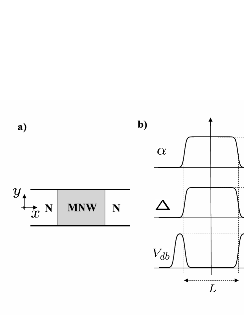
Figure 1: Sketch of the physical system. Panel a) displays our choice of coordinates while panel b) shows the longitudinal variation of the Hamiltonian parameters.

A distinctive characteristic of our model is the continuity of the system parameters with respect to the longitudinal coordinate $x$, as sketched in Fig. 1b. This would allow us to investigate, for instance, the dependence on the diffusivity $d$ of the transition. In this work, however, we will assume rather steep transitions of the system parameters. The coherent quasiparticle transport is described by the BdG equation

$${\cal H}_{BdG}\Psi=E\Psi\;,$$ (4)

where $E$ and $\Psi$ are the quasiparticle energy and wave function, respectively. The latter depends on the position in space $(x,y)$ as well as on the spin and isospin variables $(\eta_{\sigma},\eta_{\tau})$, where $\eta=\uparrow,\downarrow$ represents a generic discrete variable with only two possible values,

$$\Psi\Rightarrow\Psi(x,y,\eta_{\sigma},\eta_{\tau})\;.$$ (5)

Notice, finally, that $\hat{n}$ is assumed to lie in the $xy$ plane. An out-of-plane component would require the addition of orbital magnetic effects not considered in this work.

3 The coupled channel model

We present in this section the description of transport in terms of channel amplitudes or wave functions obeying a set of coupled differential equations. This description can be viewed as an alternative to the matching of bulk solutions often used in the literature. The CCM is well suited to the problem of a spatially continuous Hamiltonian posed in the preceding section. Before discussing the CCM equations, however, we need to consider the asymptotic solutions ($x\to\pm\infty$) as they are actually defining the channels themselves.

3.1 Asymptotic solutions

Since the pairing and Rashba intensities vanish asymptotically, the BdG Hamiltonian greatly simplifies in those regions,

$$\lim_{x\to\pm\infty}{\cal H}_{BdG}=(h_{0}-\mu)\tau_{z}+\Delta_{B}\vec{\sigma}\cdot\hat{n}\;.$$ (6)

In this limit the eigenstates are spinors pointing in the direction of $\hat{n}$ and $\hat{z}$ for spin and isospin. Introducing the quantum numbers $s_{\sigma}=\pm 1$ and $s_{\tau}=\pm 1$ they read, respectively,

$$\chi_{s_{\sigma}}\equiv\frac{1}{\sqrt{2}}\left(\begin{array}[]{c}1\\ s_{\sigma}e^{i\varphi}\end{array}\right)\quad;\quad\chi_{s_{\tau}}\equiv\frac{1}{2}\left(\begin{array}[]{c}1+s_{\tau}\\ 1-s_{\tau}\end{array}\right)\;,$$ (7)

where $\varphi$ is the azimuthal angle of $\hat{n}$. The spatial dependence of the asymptotic eigenstates is also analytical, a plane wave in $x$ and a square well eigenfunction in $y$, $\phi_{n}(y)$, with $n=1,2,\dots$. Summarizing, a channel is specified by the quantum numbers $(ns_{\sigma}s_{\tau})$ and its wave function reads

$$\Psi_{ns_{\sigma}s_{\tau}}\equiv e^{ikx}\phi_{n}(y)\chi_{s_{\sigma}}(\eta_{\sigma})\chi_{s_{\tau}}(\eta_{\tau})\;.$$ (8)

The propagating or evanescent character of each channel is found when determining its wavenumber $k\equiv k_{ns_{\sigma}s_{\tau}}$. From Eq. (4) the asymptotic BdG energy is

$$E=\left(\frac{\hbar^{2}k_{ns_{\sigma}s_{\tau}}^{2}}{2m^{*}}+\varepsilon_{n}-\mu\right)s_{\tau}+\Delta_{B}s_{\sigma}\;,$$ (9)

where

$$\varepsilon_{n}=\frac{\pi^{2}n^{2}\hbar^{2}}{2m^{*}L_{y}^{2}}\;.$$ (10)

Inverting Eq. (9) it is

$$k_{ns_{\sigma}s_{\tau}}=\sqrt{\frac{2m^{*}}{\hbar^{2}}\left(Es_{\tau}-\varepsilon_{n}+\mu-\Delta_{B}s_{\sigma}s_{\tau}\right)}\;.$$ (11)

The channel wavenumber $k_{ns_{\sigma}s_{\tau}}$ from Eq. (11) is either real or purely imaginary. These two cases clearly correspond to propagating and evanescent channels, respectively. In conclusion, for electrons ($s_{\tau}=1$) and holes ($s_{\tau}=-1$) the condition for propagating mode of spin $s_{\sigma}$ in direction of $\hat{n}$ and with transverse state $n$ is

$$Es_{\tau}-\varepsilon_{n}+\mu-\Delta_{B}s_{\sigma}s_{\tau}>0\;.$$ (12)

3.2 The CCM equations

Assume the following expansion of the full wave function, valid not only in the asymptotic leads but for any arbitrary position,

$$\Psi(x,y,\eta_{\sigma},\eta_{\tau})=\sum_{ns_{\sigma}s_{\tau}}{\psi_{ns_{\sigma}s_{\tau}}(x)\phi_{n}(y)\chi_{s_{\sigma}}(\eta_{\sigma})\chi_{s_{\tau}}(\eta_{\tau})}\;,$$ (13)

where $\psi_{ns_{\sigma}s_{\tau}}(x)$ is a 1D function we call the channel amplitude. Obviously, the channel amplitudes in the asymptotic regions are $\psi_{ns_{\sigma}s_{\tau}}(x)\propto\exp{(\pm ik_{ns_{\sigma}s_{\tau}}x)}$, i.e., propagating or evanescent waves to the right or left directions, depending on the sign of the exponent. The equations fulfilled by the channel amplitudes can be obtained substituting the wave function, Eq. (13), in the BdG equation, Eq. (4), and projecting on a specific channel,

$$\sum_{\eta_{\sigma}\eta_{\tau}}\int_{0}^{L_{y}}{dy}\,\phi_{n}(y)\chi^{*}_{s_{\sigma}}(\eta_{\sigma})\chi^{*}_{s_{\tau}}(\eta_{\tau})\;\times{\left[{\cal H}_{BdG}\Psi=E\Psi\right]}\;.$$ (14)

The sets of transverse wave functions $\{\phi_{n}\}$, $\{\chi_{s_{\sigma}}\}$ and $\{\chi_{s_{\tau}}\}$ fulfills proper orthonormality relations. After some straightforward algebra, Eq. (14) leads to

$$\!\!\!\!\!\!\!\!\!\!\!\!\!\!\!\!\!\!\!\!\left[\left(\frac{p_{x}^{2}}{2m^{*}}+V_{db}(x)+\varepsilon_{n}-\mu\right)s_{\tau}+\Delta_{B}s_{\sigma}+s_{\sigma}s_{\tau}\sin\varphi\frac{1}{2\hbar}\{p_{x},\alpha(x)\}-E\right]\psi_{ns_{\sigma}s_{\tau}}(x)$$

$$+s_{\sigma}s_{\tau}\cos\varphi\frac{i}{2\hbar}\{p_{x},\alpha(x)\}\,\psi_{n\bar{s_{\sigma}}s_{\tau}}(x)+\Delta(x)\,\psi_{ns_{\sigma}\bar{s_{\tau}}}(x)$$

$$-s_{\sigma}s_{\tau}\frac{\alpha(x)}{\hbar}\sum_{n^{\prime}(\neq n)}{\langle n|p_{y}|n^{\prime}\rangle\left[\rule{0.0pt}{12.80365pt}\cos\varphi\,\psi_{n^{\prime}s_{\sigma}s_{\tau}}(x)-i\sin\varphi\,\psi_{n^{\prime}\bar{s_{\sigma}}s_{\tau}}(x)\right]}=0\;,$$ (15)

where we have introduced the usual anticommutator notation, $\{p_{x},\alpha(x)\}=p_{x}\alpha(x)+\alpha(x)p_{x}$ and the bar over an index denotes its opposite value. The set of Eqs. (3.2) is already a first version of our desired CCM equations. There are three types of contributions to Eq. (3.2): a) the background terms of channel $(ns_{\sigma}s_{\tau})$ are given by the first line, b) the second line contains the coupling terms with channels of the same $n$ but with opposite spin $\bar{s_{\sigma}}$ or isospin $\bar{s_{\tau}}$ to that of the background channel, c) finally, the third line shows the coupling with channels of a different $n$, the same isospin and arbitrary spin.

The physical role played by the different Hamiltonian contributions are clearly seen in Eq. (3.2). As expected, the superconducting pairing $\Delta(x)$ couples electron and hole channels. The two Rashba terms have a markedly different effect regarding the $n$ quantum number. The $\alpha(x)p_{x}$ is diagonal in $n$, while the $\alpha(x)p_{y}$ is mixing channels with different $n$’s with the selection rules imposed by the square well matrix element $\langle n|p_{y}|n^{\prime}\rangle$. The relevance of the field orientation is also appreciated from Eq. (3.2). For instance, if the field is along $y$ ($\varphi=\pi/2$) the mixing of $(ns_{\sigma}s_{\tau})$ and $(n\bar{s_{\sigma}}s_{\tau})$ vanishes.

We end this section mentioning a useful transformation of Eq. (3.2) that eliminates the linear terms in $p_{x}$ of the background problem. Let us define the transformed channel amplitude

$$\tilde{\psi}_{ns_{\sigma}s_{\tau}}(x)=e^{is_{\sigma}\sin\varphi\,{\cal K}_{R}(x)}\psi_{ns_{\sigma}s_{\tau}}(x)\;,$$ (16)

where we introduced the dimensionless function

$${\cal K}_{R}(x)=\frac{m^{*}}{\hbar^{2}}\int_{0}^{x}{dx^{\prime}\alpha(x^{\prime})}\;.$$ (17)

Substituting Eq. (16) into Eq. (3.2) we find

$$\!\!\!\!\!\!\!\!\!\!\left[\left(\frac{p_{x}^{2}}{2m^{*}}+V_{db}(x)+\varepsilon_{n}-\mu-\frac{m^{*}}{2\hbar^{2}}\alpha(x)^{2}\sin^{2}\varphi\right)s_{\tau}+\Delta_{B}s_{\sigma}-E\right]\tilde{\psi}_{ns_{\sigma}s_{\tau}}(x)$$ (18)

$$+ \left[s_{\tau}\cos\varphi e^{2is_{\sigma}\sin\varphi\,{\cal K}_{R}(x)}\left(i\frac{m^{*}}{\hbar^{2}}\alpha(x)^{2}\sin\varphi+s_{\sigma}\frac{i}{2\hbar}\{p_{x},\alpha(x)\}\right)\right]\,\tilde{\psi}_{n\bar{s_{\sigma}}s_{\tau}}(x)$$

$$+ \Delta(x)\,\tilde{\psi}_{ns_{\sigma}\bar{s_{\tau}}}(x)-s_{\sigma}s_{\tau}\frac{\alpha(x)}{\hbar}\sum_{n^{\prime}(\neq n)}{\langle n|p_{y}|n^{\prime}\rangle\left[\rule{0.0pt}{14.22636pt}\cos\varphi\,\tilde{\psi}_{n^{\prime}s_{\sigma}s_{\tau}}(x)\right.}$$

$$\qquad\qquad\qquad\qquad\left.\rule{0.0pt}{14.22636pt}-i\sin\varphi e^{2is_{\sigma}\sin\varphi\,{\cal K}_{R}(x)}\,\tilde{\psi}_{n^{\prime}\bar{s_{\sigma}}s_{\tau}}(x)\right]=0\;,$$

The set of Eqs. (18) is very similar to (3.2), with two important differences: a) the background channel terms have a new contribution quadratic in $\alpha(x)$ which is spin-independent, while the contribution linear in $p_{x}$ is effectively eliminated from this channel, b) the position-dependent phase of the transformation given in Eq. (16) appears explicitly in the coupling with $(n\bar{s_{\sigma}}s_{\tau})$ and $(n^{\prime}\bar{s_{\sigma}}s_{\tau})$.

3.3 The QTBM

We have solved the set of Eqs. (3.2) using the quantum-transmitting-boundary formulation of the scattering problem. The reader is addressed to Refs. [22, 23] for details on the QTBM. Here we just mention for the sake of completeness the basic underlying ideas. Using a 1D grid Eq. (3.2) can be discretized with finite-difference formulas for the derivatives. In the asymptotic regions of the leads we impose the analytical solutions of the channel amplitudes

$$\psi_{ns_{\sigma}s_{\tau}}(x)=a^{(i)}_{ns_{\sigma}s_{\tau}}e^{is_{i}s_{\tau}k_{ns_{\sigma}s_{\tau}}(x-x_{i})}+b^{(i)}_{ns_{\sigma}s_{\tau}}e^{-is_{i}s_{\tau}k_{ns_{\sigma}s_{\tau}}(x-x_{i})}\;,$$ (19)

where $a^{(i)}_{ns_{\sigma}s_{\tau}}$ and $b^{(i)}_{ns_{\sigma}s_{\tau}}$ are the usual incident and reflected amplitudes in lead $i$. In Eq.  (19) we have introduced the lead sign $s_{i}$, equal to +1 and $-1$ for the left ($i=1$) and right ($i=2$) leads, respectively, as well as the position of each lead boundary $x_{i}$. We have also taken into account the reversed direction of propagation for electrons and holes with the $s_{\tau}$ sign. Notice that from Eq. (19) the outgoing coefficient $b^{(i)}_{ns_{\sigma}s_{\tau}}$ is expressed in terms of the channel amplitude at the lead boundary, $b^{(i)}_{ns_{\sigma}s_{\tau}}=\psi_{ns_{\sigma}s_{\tau}}(x_{i})-a^{(i)}_{ns_{\sigma}s_{\tau}}$. Substituting this explicit expression of $b^{(i)}_{ns_{\sigma}s_{\tau}}$ back in Eq. (19) we obtain

$$\!\!\!\!\!\!\!\!\!\!\!\!\!\!\!\psi_{ns_{\sigma}s_{\tau}}(x)-e^{-is_{i}s_{\tau}k_{ns_{\sigma}s_{\tau}}(x-x_{i})}\psi_{ns_{\sigma}s_{\tau}}(x_{i})=2i\sin{\left(s_{i}s_{\tau}k_{ns_{\sigma}s_{\tau}}(x-x_{i})\right)}a^{(i)}_{ns_{\sigma}s_{\tau}}\\ \;.$$ (20)

The QTBM closed system of linear equations is defined as follows: a) for a grid point $x$ such that $x_{1}\leq x\leq x_{2}$ we impose the discretized version of Eq. (3.2), b) for a grid point having $x<x_{1}$ or $x>x_{2}$ we impose Eq. (20). The resulting linear system has as many equations as grid points and it depends only on the set of input coefficients $\{a^{(i)}_{ns_{\sigma}s_{\tau}}\}$. It is highly sparse and can be numerically solved in an efficient way.

The matrix of transmissions from mode $ns_{\sigma}s_{\tau}$ of lead $i$ to mode $n^{\prime}s^{\prime}_{\sigma}s^{\prime}_{\tau}$ of lead $i^{\prime}$ is given by

$$t(i^{\prime}n^{\prime}s^{\prime}_{\sigma}s^{\prime}_{\tau}\leftarrow ins_{\sigma}s_{\tau})=\left.\frac{\sqrt{k_{n^{\prime}s^{\prime}_{\sigma}s^{\prime}_{\tau}}}\,b^{(i^{\prime})}_{n^{\prime}s^{\prime}_{\sigma}s^{\prime}_{\tau}}}{\sqrt{k_{ns_{\sigma}s_{\tau}}}\,a^{(i)}_{ns_{\sigma}s_{\tau}}}\right|_{\rm oim}\;,$$ (21)

where the subscript oim, standing for only incident mode, refers to the fact that all incident amplitudes vanish except the one explicitly appearing in the denominator of Eq. (21). For use in the next section, we define a reduced matrix of transmission probabilities where we only discriminate lead and particle type,

$$P_{i^{\prime}i}^{s^{\prime}_{\tau}s_{\tau}}=\sum_{nn^{\prime}s_{\sigma}s^{\prime}_{\sigma}}{\left|\,t(i^{\prime}n^{\prime}s^{\prime}_{\sigma}s^{\prime}_{\tau}\leftarrow ins_{\sigma}s_{\tau})\,\right|^{2}}\;.$$ (22)

4 Transport in the BdG framework

The description of transport through MNW’s can be done with the formalism of transport through normal/superconductor/normal structures. We follow, specifically, the formulation by Lambert et al. [21] for mesoscopic superconductors. For our two-terminal structure, labelled as $i=1,2$ for left and right contacts, the current in terminal $i$ reads

$$I_{i}=\int_{0}^{\infty}{\sum_{\alpha=\pm 1}{\alpha\left(J_{i}^{\alpha}(E)-\hat{J}_{i}^{\alpha}(E)\right)}\,dE}\;,$$ (23)

where $E$ is the BdG quasiparticle energy. In Eq. (23), $J_{i}^{\alpha}(E)$ and $\hat{J}_{i}^{\alpha}(E)$ are, respectively, the in-going and out-going fluxes in lead $i$ of type $\alpha$.

The essential ingredients we need to specify in order to use Eq. (23) are the quasiparticle energy distributions $f_{i}^{\alpha}(E)$, the number of propagating modes $m_{i}^{\alpha}(E)$, and the matrix of quantum transmissions $P_{ij}^{\alpha\beta}(E)$. The latter two are obtained from the CCM, Eqs. (12) and (22), respectively. The quasiparticle distributions are assumed to be given by Fermi functions

$$f_{i}^{\alpha}(E)=\left[1+e^{\left(E-\alpha eV_{i}\right)/KT}\right]^{-1}\;,$$ (24)

where the $i$-th reservoir chemical potential has been defined as $\mu_{i}=\mu+eV_{i}$ and $kT$ is the thermal energy. With these inputs the fluxes in Eq. (23) read

$$J_{i}^{\alpha}(E) = \frac{e}{h}m_{i}^{\alpha}(E)f_{i}^{\alpha}(E)\;,$$ (25)

$$\hat{J}_{i}^{\alpha}(E) = \frac{e}{h}\sum_{j\beta}P_{ij}^{\alpha\beta}(E)f_{j}^{\beta}(E)\;.$$ (26)

This formalism fulfills two basic physical conditions: a) vanishing of current for zero bias and b) equality of current in both leads. Indeed, for zero bias all distributions are identical $f_{i}^{\alpha}(E)\equiv f(E)$ and then the sum rule on quantum transmissions,

$$\sum_{j\beta}{P_{ij}^{\alpha\beta}(E)}=m_{i}^{\alpha}(E)\;,$$ (27)

ensures that in-going and out-going fluxes exactly cancel each other. The second condition, $I_{1}+I_{2}=0$, is more subtle; following Lambert [21] we interpret that it actually determines the MNW chemical potential $\mu$, relative to $\mu_{1}$ and $\mu_{2}$. Notice that the potential bias between the two leads is $V=V_{1}-V_{2}$ and that the MNW chemical potential lies somewhere in the range between the two reservoir chemical potentials,

$$\min(\mu_{1},\mu_{2})\leq\mu\leq\max(\mu_{1},\mu_{2})\;.$$ (28)

The following practical approach to the BdG transport problem is then suggested: 1) given $\mu_{1}$ and $\mu_{2}$, assume $\mu=(\mu_{1}+\mu_{2})/2$ and solve the BdG-CCM equations for the set $\{m_{i}^{\alpha},P_{ij}^{\alpha\beta}\}$; 2) compute $I_{1}+I_{2}$; 3) vary the value of $\mu$ and recompute $\{m_{i}^{\alpha},P_{ij}^{\alpha\beta}\}$ until $I_{1}+I_{2}=0$ is fulfilled. Solving this selfconsistency loop might be a difficult task, however it is not needed when the problem is symmetric with respect to $x$ inversion around the center of the MNW. In this case $\mu=(\mu_{1}+\mu_{2})/2$ is already the solution giving $I_{1}+I_{2}=0$ since the bias $V$ has to be shared symmetrically, $V_{i}=s_{i}V/2$, where $s_{1}=1$ and $s_{2}=-1$. Here we shall focus on the symmetric problem, leaving for a future work the analysis on the non symmetric case.

4.1 Differential and linear conductances

The differential conductance, defined generically as $dI/dV$, is one of the most relevant transport properties usually measured in experiments. At zero temperature, the above formalism yields a very simple expression of this quantity because, in this limit, the derivatives of the quasiparticle distribution functions with respect to the bias become Dirac deltas. Of course, this is true only in the symmetric case, when $V=2s_{i}V_{i}$.

For $T=0$ we obtain

$$\frac{dI_{1}}{dV}=\frac{e^{2}}{2h}\left(P_{12}^{++}({\scriptstyle\frac{1}{2}}eV)+P_{12}^{--}({\scriptstyle\frac{1}{2}}eV)+P_{11}^{+-}({\scriptstyle\frac{1}{2}}eV)+P_{11}^{-+}({\scriptstyle\frac{1}{2}}eV)\right)\;,$$ (29)

and, as discussed above, it is $dI_{2}/dV=-dI_{1}/dV$. The expression of the linear conductance $G$ can be obtained simply setting the bias to zero in Eq. (29). Using, in addition, the particle hole symmetry

$$P_{ij}^{\alpha\beta}(E)=P_{ij}^{\bar{\alpha}\bar{\beta}}(-E)\;,$$ (30)

we find

$$G=\frac{e^{2}}{h}\left(P_{12}^{++}(0)+P_{11}^{+-}(0)\right)\;.$$ (31)

Equations (29) and (31) are the basic relations of this work. Notice that they contain two qualitatively different contributions to the conductance, a normal transmission, $T_{0}\equiv(P_{12}^{++}+P_{12}^{--})/2$, whereby quasiparticle type is conserved; and an Andreev reflection, $R_{A}\equiv(P_{11}^{+-}+P_{11}^{-+})/2$, with quasiparticle change. Anticipating a result to be discussed below, notice that Eqs. (29) and (31) predict a remarkable phenomenon, a nonvanishing conductance in absence of transmission ($T_{0}=0$) due solely to Andreev reflection. This occurs when the Majorana nanowire has a zero mode. In this case Andreev reflection is maximal for zero bias, while increasing the bias there is a reduction of $R_{A}$, i.e., a zero-bias anomaly appears in $dI_{1}/dV$ due to the zero mode.

5 Results and discussion

5.1 Physical and scaled values of the parameters

The relative strengths of spin-orbit, pairing and Zeeman terms for a given transverse dimension $L_{y}$ are determined by the following scaled dimensionless ratios (scaling is indicated with an $s$ superscript)

$$\alpha_{0}^{(s)} = \frac{\alpha_{0}m^{*}}{\hbar^{2}}L_{y}\;,$$ (32)

$$\Delta_{0}^{(s)} = \frac{\Delta_{0}m^{*}}{\hbar^{2}}L_{y}^{2}\;,$$ (33)

$$\Delta_{B}^{(s)} = \frac{\Delta_{B}m^{*}}{\hbar^{2}}L_{y}^{2}\;.$$ (34)

Notice that for a given set of physical values of $\alpha_{0}$, $\Delta_{0}$ and $\Delta_{B}$ different values of the transverse dimension $L_{y}$ will actually correspond to different relative strengths through Eqs. (32-34). Increasing $L_{y}$ the scenario clearly evolves from weak to strong couplings.

More specifically, we consider below physical parameters that could represent an InAs-based nanowire [24], $m^{*}=0.033m_{e}$, $\alpha_{0}=30$ meVnm and a pairing gap of $\Delta_{0}=0.3$ meV. We assume a realistic value of the wire transverse dimension, $L_{y}=150$ nm, for which the relative strengths of Rashba and pairing are then $\alpha_{0}^{(s)}\approx 2$ and $\Delta_{0}^{(s)}\approx 3$. Fixing these two scaled parameters to these values we will study the dependence on the third one $\Delta_{B}^{(s)}$ below. The conversion of the Zeeman coupling to a physical magnetic field is $B=\Delta_{B}/g\mu_{B}$, with $g$ and $\mu_{B}$ the g factor and Bohr magneton, respectively. With our assumptions this conversion reads $B=(1.7\Delta_{B}^{(s)}/g)$ T, in terms of the scaled Zeeman coupling. That is, $B=1$ T would correspond to $\Delta_{B}^{(s)}=10$ for a g factor $\approx 17$.

The distance $L$ between barriers (Fig. 1) is taken as $L=20L_{y}=3$ $\mu{\rm m}$, with barrier thickness of 150 nm and height $V_{0}=0.5$ meV, while the spatial diffusivity is $d=15$ nm [see, e.g., Eq. (3)]. We also choose the chemical potential, defining our reference energy of the MNW, as $\mu=0$. Overall, we stress that the complete parameter set is representative of a typical experiment with an InAs-based 2D semiconductor wire.

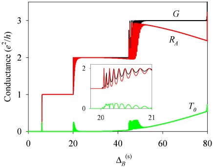
Figure 2: (Colour online) Linear conductance in absence of Rashba mixing as a function of the scaled Zeeman energy. The contributions from Andreev reflection ($R_{A}$) and normal transmission ($T_{0}$) are also shown. The inset shows a blow-up of the data in a small region. The system parameters are given in Subsection 5.1.

5.2 Linear conductance results

In Figs. 2 to 4 we display the linear conductance calculated from Eq. (31) as a function of the scaled Zeeman value $\Delta_{B}^{(s)}$ for the set of parameters mentioned in the preceding subsection. Figures 2 and 3 correspond to magnetic field in parallel direction to the wire ($x$) while Fig. 4 is for transverse orientation ($y$). In Figure 2 we neglected the contribution of the Rashba mixing, i.e., of the terms containing $\alpha(x)p_{y}$ in Eq. (3.2). Notice that in this situation the linear conductance displays an almost perfect quantization in $e^{2}/h$ steps. Increasing $\Delta_{B}^{(s)}$, small deviations in the form of very narrow spikes can be seen at the beginning of the second and third plateaus. In the first two steps all the conductance is due to Andreev reflection since the normal transmission is negligible. Perfect Andreev reflection is a signal of the existence of a zero mode of the closed system, i.e., a Majorana fermion bound at the interface between the MNW and the normal contacts. This zero mode yields a perfectly quantized conductance in absence of transmission due solely to Andreev reflection, i.e., $G=(e^{2}/h)R_{A}$. The decrease of Andreev reflection for $\Delta_{B}^{(s)}>50$ in Fig. 2 can be attributed to the finite size effect that removes the Majorana modes from perfect zero energy, in agreement with the analysis of Ref. [26] for the closed system. This decrease in $R_{A}$ is accompanied by an increase in $T_{0}$, keeping the value of $G$ close to integer multiples of $e^{2}/h$, except at the transition between steps.

Figure 3 displays the linear conductance for the same system of Fig. 2, but now including the full Rashba interaction. A conspicuous difference with Fig. 2 is that the conductance deviates from the simple staircase behaviour, with a broad conductance dip appearing at the end of the first plateau. This dip is due to a magnetic instability precluding the formation of two zero modes due to a repulsion between modes induced by Rashba mixing [26]. The effect of this mechanism on the linear conductance is remarkable, with the prediction of a reduced conductance due to a large reduction of Andreev reflection. This anomalous behaviour of the conductance at the end of the conductance plateau also appears in higher plateaus, as seen in Fig. 3 for the second and third plateaus. Notice, however, that the finite size effect mentioned above transforms the conductance dips of the higher plateaus in a strongly oscillating behaviour. We have checked that the formation of the conductance dips due to the instability of multiple zero modes is even more robust with higher values of the pairing gap and Rashba strengths, and that it is also robust against variations of the barriers between the normal contacts and the MNW.

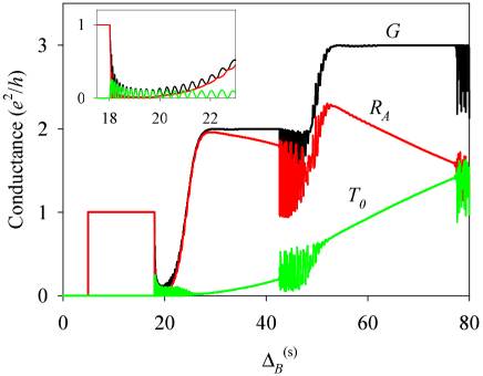
Figure 3: (Colour online) Same as Fig. 2 including Rashba mixing.

Figure 4 shows the evolution of the linear conductance with $\Delta_{B}^{(s)}$ for field along the transverse direction $y$. For this orientation of the field the physics changes completely, since now it is the Andreev reflection that vanishes and the conductance is due to the normal transmission. Only small peaks in $R_{A}$ can be seen in the transition between plateaus. The vanishing of $R_{A}$ is due to the absence of zero modes of the closed MNW for magnetic fields along $y$ [26]. A similar orientation anisotropy has been seen in experiments with cylindric InSb nanowires [4, 5]. No conductance dips are observed in Fig. 4 but there are many spikes due to resonant transmission through the double-barrier potential $V_{db}(x)$. The separation between spikes is very small due to the dense distribution of quasibound states for such a long system $L=3$ $\mu$m. From this point of view, it is still more remarkable the fact that for field along $x$ the presence of a zero mode washes the spike oscillations and yields a consistent maximal conductance in some regimes.

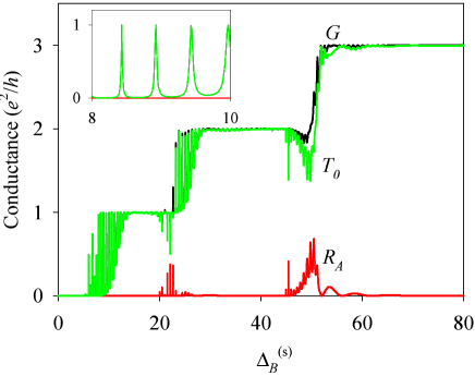
Figure 4: (Colour online) Same as Fig. 3 for magnetic field along $y$.

5.3 Nonlinear conductance

The nonlinear conductance obtained with Eq. (29) is shown in Fig. 5 as a function of the applied bias. We have taken some selected values of $\Delta_{B}^{(s)}$ from Fig. 3, corresponding to vanishing bias, and explored the variation with $V$. As in the preceding subsection we define a scaled bias taking the transverse confinement as reference, i.e., $V^{(s)}=(em^{*}L_{y}^{2}/\hbar^{2})V$. For $\Delta_{B}^{(s)}=9$ there is a narrow peak in $dI_{1}/dV$ at zero bias. This zero bias anomaly is reflecting the existence of a zero mode in the MNW. Increasing the Zeeman coupling the peak broadens, becoming a flat distribution. For $\Delta_{B}^{(s)}=19$, corresponding to the conductance dip of Fig. 3, the zero bias peak changes to a zero bias minimum. The existence of a zero bias anomaly in the presence of zero modes has been discussed before in systems with a superconductor contact, experimentally in Refs. [4, 5] and theoretically in Refs. [15, 16, 17]. Our results prove that a similar behaviour is to be expected in N/MNW/N structures.

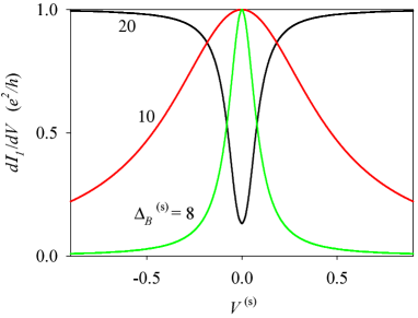
Figure 5: (Colour online) $dI_{1}/dV$ as a function of scaled bias $V^{(s)}$ for the same parameters of Fig. 3 and for different values of $\Delta_{B}^{(s)}$.

5.4 Density distributions

The density distributions, defined as $|\psi_{ns_{\sigma}s_{\tau}}(x)|^{2}$, are shown in Fig. 6 for two values of $\Delta_{B}^{(s)}$. They correspond to the perfect Andreev reflection ($\Delta_{B}^{(s)}=10$) and to the conductance dip ($\Delta_{B}^{(s)}=19$) of Fig. 3. As expected, the upper panel shows that the incident unitary density couples with an edge mode of the MNW. The density profile localized at the edge and decaying towards the interior has exactly the same shape found in calculations of zero modes of closed MNW’s [26]. Perfect Andreev reflection in this situation consists in the total reflection in the conjugate channel and, therefore, no quantum interference is observed in the left contact. As mentioned before, this occurs due to the presence of the zero mode in the MNW and it allows unit conductance without any transmission at all between left and right contacts.

The lower panel of Fig. 6 shows a qualitatively different behaviour. The beating pattern in the left contact is indicating that full reflection occurs now in the same channel of incidence, with a strong interference between incident and reflected waves The density at the edge of the MNW is more irregular and extends farther towards the interior than in the upper panel. The physical interpretation is clear: for this Zeeman intensity the edge mode of the MNW lies at a nonzero energy, this causing normal reflection, as opposed to the Andreev reflection of the upper panel.

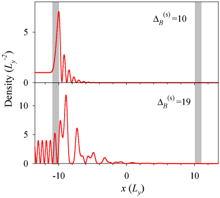
Figure 6: Density distributions $|\psi_{ns_{\sigma}s_{\tau}}(x)|^{2}$ for two values of $\Delta_{B}^{(s)}$ of the first plateau of Fig. 3. We assumed boundary conditions corresponding to incidence from the left side. For comparison, the position of the potential barriers is indicated by the shaded regions.

6 A model in second quantization

To provide additional insight on the physics of transport through the MNW, in this section we consider an effective Hamiltonian in second quantization projected onto the Majorana subspace. The Hamiltonian consists of three parts, that is,

$${\cal{H}}_{\it eff}={\cal{H}}_{C}+{\cal{H}}_{M}+{\cal{H}}_{T}\;,$$ (35)

with

$${\cal{H}}_{C} = \sum_{\alpha=L/R,k}\varepsilon_{\alpha k}c_{\alpha k}^{{\dagger}}c_{\alpha k}\;,$$ (36a)

$${\cal{H}}_{M} = \frac{i}{2}\varepsilon_{M}\eta_{L}\eta_{R}\;,$$ (36b)

$${\cal{H}}_{T} = \sum_{\alpha,\beta,k}\left(V_{\alpha k,\beta}^{\ast}c_{\alpha k}^{{\dagger}}\eta_{\beta}+V_{\alpha k,\beta}\eta_{\beta}c_{\alpha k}\right)\;.$$ (36c)

Here ${\cal{H}}_{C}$ describes the normal leads, with $c_{\alpha k}^{{\dagger}}$ ($c_{\alpha k}$) the Dirac fermion creation (annihilation) operator. Notice that the spin degree of freedom is neglected. This can be understood considering that we need to apply a large magnetic field to observe the edge Majoranas, so that only one kind of spin is effectively involved [25]. ${\cal{H}}_{M}$ characterizes the coupled Majorana states, with $\eta_{L/R}$ Majorana fermion operators fulfilling $\eta_{i}=\eta_{i}^{{\dagger}}$, $\eta_{i}^{2}=1$ and with anticommutator relation $\{\eta_{i},\eta_{j}\}=2\delta_{ij}$. The parameter $\varepsilon_{M}$ denotes the coupling between the two Majoranas on opposite ends of the MNW and can be some complicated function of wire length, superconducting coherence length, applied magnetic field, Rashba coupling and superconducting gap. $\varepsilon_{M}$ might be found by exact diagonalization of Hamiltonian (1) [26]. We will assume that it is known for the purpose of the present model. The last contribution, ${\cal{H}}_{T}$, corresponds to the tunnel Hamiltonian between normal leads and the Majoranas on opposite ends [16]. Below, the tunnel amplitude $V_{\alpha k,\beta}$ is taken as $V$ for $\alpha=\beta$ and zero for $\alpha\neq\beta$.

The current is computed from

$$I_{\alpha}=-\frac{ie}{\hbar}\langle[{\cal{H}},n_{\alpha}]\rangle=-\frac{2e}{\hbar}\Re\left\{\sum_{\beta}\sum_{k\in\alpha}V_{\alpha k,\beta}{\cal{G}}_{\alpha k,\beta}^{<}(t,t)\right\}\;,$$ (36ak)

where $n_{\alpha}=\sum_{k\in\alpha}c_{\alpha k}^{{\dagger}}c_{\alpha k}$ and ${\cal{G}}_{\alpha k,\beta}^{<}$ denotes the lesser component of the mixed Green’s function defined as

$${\cal{G}}_{\alpha k,\beta}(t,t^{\prime})=-i\langle T_{K}c_{\alpha k}(t)\eta_{\beta}(t^{\prime})\rangle\;.$$ (36al)

Employing the equation of motion technique, after tedious algebra, the current becomes

$$I_{\alpha}=-\frac{2e}{\hbar}\Im\left\{\int d\varepsilon~{}\Tr\left[f_{\alpha}(\varepsilon)\left({\mathbf{\cal{G}}}_{\eta}^{r}(\varepsilon)-{\mathbf{\cal{G}}}_{\eta}^{a}(\varepsilon)\right)\mathbf{\Gamma}_{\alpha}(\varepsilon)+{\mathbf{\cal{G}}}_{\eta}^{<}(\varepsilon)\mathbf{\Gamma}_{\alpha}(\varepsilon)\right]\right\}\;,$$ (36am)

where ${\mathbf{\cal{G}}}_{\eta}(\varepsilon)$ is the Green’s function for the MNW and $\mathbf{\Gamma}_{\alpha}(\varepsilon)$ denotes the hybridization matrix given by

$$\mathbf{\Gamma}_{\alpha;\beta\gamma}(\varepsilon)=\pi\sum_{k\in\alpha}V_{\alpha k,\beta}V_{\alpha k,\gamma}^{\ast}\delta(\varepsilon-\varepsilon_{\alpha k})=\delta_{\alpha,\beta}\delta_{\beta,\gamma}\Gamma/2\;.$$ (36an)

To complete the calculation we need to determine the MNW Green’s functions. They read [16]

$${\mathbf{\cal{G}}}_{\eta}^{r/a}(\varepsilon) =\frac{2}{\varepsilon-i\mathbf{t}-2\mathbf{\Sigma}_{0}^{r/a}(\varepsilon)}\;,$$ (36ao)

$${\mathbf{\cal{G}}}_{\eta}^{<}(\varepsilon) ={\mathbf{\cal{G}}}_{\eta}^{r}(\varepsilon)\mathbf{\Sigma}_{0}^{<}(\varepsilon){\mathbf{\cal{G}}}_{\eta}^{a}(\varepsilon)\;.$$ (36ap)

Here,

$$\mathbf{t}=\left(\begin{array}[]{cc}0&\varepsilon_{M}\\ -\varepsilon_{M}&0\end{array}\right)\;,$$ (36aq)

and the self-energy matrices are given by

$$\mathbf{\Sigma}_{0;\alpha\beta}^{r/a}(\varepsilon) =\mp i\sum_{\gamma}\left[\mathbf{\Gamma}_{\gamma;\alpha\beta}(\varepsilon)+\mathbf{\Gamma}_{\gamma;\beta\alpha}(-\varepsilon)\right]\;,$$ (36ar)

$$\mathbf{\Sigma}_{0;\alpha\beta}^{<}(\varepsilon) =2i\sum_{\gamma}\left[f_{\gamma}(\varepsilon)\mathbf{\Gamma}_{\gamma;\alpha\beta}(\varepsilon)+f_{\gamma}(-\varepsilon)\mathbf{\Gamma}_{\gamma;\beta\alpha}(-\varepsilon)\right]\;.$$ (36as)

Substituting Eqs. (36an)-(36as) into Eq. (36am) and using current conservation we obtain

$$\!\!\!\!\!\!\!\!\!\!\!\!\!\!\!\!\!\!\!\!\ I_{L}=-I_{R}=\frac{e}{h}\int d\varepsilon~{}\frac{4\Gamma^{2}\left(\varepsilon^{2}+4\Gamma^{2}+\varepsilon_{M}^{2}\right)}{\left(\varepsilon^{2}+4\Gamma^{2}\right)^{2}+\varepsilon_{M}^{2}\left(\varepsilon_{M}^{2}-2\left(\varepsilon^{2}-4\gamma^{2}\right)\right)}\left(f_{L}(\varepsilon)-f_{R}(\varepsilon)\right)\;.$$ (36at)

From Eq.  (36at) we note that at $T=0$ the linear conductance finally reads

$$G=\frac{e^{2}}{h}\frac{4\Gamma^{2}}{\varepsilon_{M}^{2}+4\Gamma^{2}}\;.$$ (36au)

For zero energy Majoranas $\varepsilon_{M}=0$ and then Eq.  (36at) yields $G=e^{2}/h$. This result nicely agrees with our interpretation of Fig. 3 attributing maximal conductance to the zero mode.

7 Conclusions

We have presented the formalism of transport in a N/MNW/N structure based on the coupled channel model. This formalism yields a transparent interpretation of the coupling between channels induced by the relevant physical mechanisms of the problem. Namely, the confinement, Zeeman, Rashba and superconducting interactions. We have considered a 2D structure and in-plane magnetic fields, although the formalism can be extended to consider more spatial dimensions and different geometries.

The coupled-channel-model equations have been solved using the quantum-transmitting-boundary algorithm for a set of parameters representative of an InAs nanowire. The existence of a zero mode in the MNW is characterized by a perfect Andreev reflection, whereby an incident channel is totally reflected in its antiparticle conjugate one. For a single zero mode the linear conductance takes the maximal value $e^{2}/h$ due solely to Andreev reflection, without any quantum transmission from left to right contacts. For increasing values of the Zeeman coupling along the wire, a conspicuous dip in the linear conductance is predicted due to repulsion between Majoranas. This repulsion originates in the Rashba mixing between channels. On the contrary, for Zeeman coupling along $y$ the Andreev reflection vanishes, with the possible exception of a small region close to the transition between plateaus. When the zero mode is absent, the linear conductance has narrow spikes as a function of the Zeeman coupling.

The differential conductance signals the presence of the zero mode with a peak at zero bias. The zero bias peak evolves to a dip when the MNW zero mode is absent. Finally, we have also discussed an effective model in second quantization confirming the physical interpretation in terms of Majorana modes. The coupled channel model presented in this work can be used to investigate other scenarios like, e.g., non-symmetric barriers or sequential MNW’s. Work along these lines is in progress.

References

References

- [1] Sau J D, Lutchyn R M, Tewari S, Das Sarma S 2010 Phys. Rev. Lett.104, 040502
- [2] Alicea J 2010 Phys. Rev.B 81, 125318
- [3] Oreg Y, Refael G, von Oppen F 2010 Phys. Rev. Lett.105, 177002
- [4] Mourik V, Zuo K, Frolov S M, Plissard S R, Bakkers E P A M, Kouwenhoven L P 2012 Science 336 1003
- [5] Deng M T, Yu C L, Huang G Y, Larsson M, Caroff P, Xu H Q 2012 preprint (ArXiv:1204.4130)
- [6] Rokhinson L P, Liu X, Furdyna J K 2012 preprint (ArXiv: 1204.2112)
- [7] Wilczek F 2009 Nat. Phys. 5 614
- [8] Franz M 2010 Physics 3, 24
- [9] Beenakker, preprint (ArXiv:1112.1950)
- [10] Alicea J, preprint (ArXiv:1202.1293)
- [11] Nadj-Perge S, Frolov S, Bakkers E P A M, Kouwenhoven L 2010 Nature 468 1084
- [12] Nilsson H A, Caroff P, Thelander C, Larsson M, Wagner J B, Wernersson L E, Samulesson L, Xu H Q 2009 Nanoletters 9 3151
- [13] Nilsson H A, Samuelson P, Caroff P, Xu H Q 2012 Nanoletters 12 228
- [14] Fu L, Kane C 2008 Phys. Rev. Lett.100, 096407
- [15] Law K T, Lee P A, Ng T K 2009 Phys. Rev. Lett.103 237001
- [16] Flensberg K 2010 Phys. Rev.B 82 180516
- [17] Wimmer M, Akhmerov A R, Dahlhaus J P, Beenakker C W J 2011 New Journal of Physics 13 053016
- [18] Akhmerov A R, Dahlhaus J P, Hassler F,Wimmer M, Beenakker C W J 2010 Phys. Rev. Lett.106, 057001
- [19] Beenakker C W J 1994 Lectures at the Les Houches summer school, Session LXI Mesoscopic Quantum Physics Akkermans E, Montambaux G, Pichard J L Eds. (North-Holland, Amsterdam)
- [20] Kitaev A Y 2001 Phys. Usp. 44 131
- [21] Lambert C J, Hui V C, Robinson S J 1993 J. Phys.: Condens. Matter5 4187
- [22] Lent C S, Kirkner D J 1990 J. Appl. Phys.67, 6353
- [23] Sánchez D, Serra L 2006 Phys. Rev.B 74, 153313
- [24] Estévez Hernández S, Akabori M, Sladek K, Volk Ch, Alagha S, Hardtdegen H, Pala M G, Demarina N, Grützmacher D, Schäpers Th 2010 Phys. Rev.B 82, 235303 (2010)
- [25] Flensberg K 2011 Phys. Rev.Lett. 106, 090503
- [26] Lim J S, López R, Serra L., Aguado R, 2012 preprint (arXiv:1202.5057)