Application of compressed sensing to the simulation of atomic systems
Abstract
Compressed sensing is a method that allows a significant reduction in the number of samples required for accurate measurements in many applications in experimental sciences and engineering. In this work, we show that compressed sensing can also be used to speed up numerical simulations. We apply compressed sensing to extract information from the real-time simulation of atomic and molecular systems, including electronic and nuclear dynamics. We find that for the calculation of vibrational and optical spectra the total propagation time, and hence the computational cost, can be reduced by approximately a factor of five.
I Introduction
A recent development in the field of data analysis is the compressed sensing (CS) (or compressive sampling) method Candes et al. (2006); Donoho (2006). The foundation of the method is the concept of sparsity: a signal expanded in a certain basis is said to be sparse when most of the expansion coefficients are zero. This extra information can be used by the CS method to significantly reduce the number of measurements needed to reconstruct a signal. CS has been successfully applied to data acquisition in many different areas Baraniuk et al. (2010). For example, to improve the resolution of medical magnetic-resonance imaging Lustig et al. (2007). It has also been applied to the experimental study of atomic and quantum systems Shabani et al. (2011); AlQuraishi and McAdams (2011); Katz et al. (2010).
In this article we show that CS can also be an invaluable tool for some numerical simulations where the optimal sampling of CS is reflected in a considerable reduction of the computational cost. We focus on atomistic simulations of nanoscopic systems by using CS to extract frequency-resolved information from real-time methods such as molecular dynamics (MD) and real-time electron dynamics.
In MDRapaport (1995); Allen and Tildesley (1989) the trajectory of the atomic nuclei is obtained by integrating their equations of motion with an interaction obtained from parametrized force-fields or by explicitly modeling the electrons Marx and Hutter (2009). Many static and dynamical properties can be obtained from MD, making it one of the most widely used methods to study atomistic systems computationally. As such it is important to develop methods that can improve the precision and reduce the computational cost of this method, especially for ab-initio MD.
While not as widely used as MD, real-time electron dynamics, in particular real-time time-dependent density functional theory (TDDFT) Runge and Gross (1984), is an important approach to study linear and non-linear electronic response Yabana and Bertsch (1996); Castro et al. (2004a, b); Takimoto et al. (2007). Due to the scalability and parallelizability properties real-time TDDFT is particularly efficient for large electronic systems Andrade et al. (2012), so an additional reduction in the computational cost can push the boundaries of the system-sizes that can be studied.
Many physical properties are represented by frequency-dependent quantities. To obtain these from a real-time framework usually a discrete Fourier transform (FT) is used. Our approach is to replace this FT by a calculation of the Fourier coefficients based on the CS method. To obtain a given frequency resolution, the CS method requires a total propagation time that is several times smaller than that required by a FT.
CS has the potential to provide across-the-board speedup for many applications involving the computation of sparse spectra. Moreover, this speedup may be obtained without making any changes to the underlying propagation code used in different types of electronic and nuclear calculations; one simply replaces the FT algorithm with the CS method, making the approach quite straightforward to implement. This paper introduces CS and demonstrates its broad utility in computational chemistry and physics by applying it to the calculation of various nuclear and electronic spectra of small molecules. The resulting computer code is available as open-source software.
The article is structured as follows. We first introduce the CS method and show how it may be applied to the determination of Fourier coefficients. Next, we apply CS to the calculation of vibrational, optical absorption, and circular dichroism spectra. We then proceed to a discussion of the numerical methods used in our CS implementation. Finally, we offer conclusions and an outlook.
II Compressed sensing
In this section, we briefly introduce the application of the CS method to the calculation of Fourier coefficients. More details about the method and its origins may be found in Refs. Baraniuk (2007); Candes and Wakin (2008); Chartrand et al. (2010).
For simplicity, we assume that we want to calculate a certain frequency-resolved quantity that is given by the sine transform of a certain time-resolved function
| (1) |
(the analysis is equally valid for the cosine transform). Since we are interested in numerical solutions, we need to think in terms of discrete quantities. In this case we want to obtain a series of values at equidistant frequencies , from the known set of time-resolved values given at equidistant times .
In principle, the set can be directly obtained using the discrete FT,
| (2) |
However, if we expect that many of the Fourier coefficients are zero, a property known as sparsity, we can use this additional information to obtain more precise results. This is the basis for the CS scheme.
We start by reformulating the discrete Fourier transform in eq. (2) as a matrix inversion problem. From this perspective, we are trying to solve the linear equation for ,
| (3) |
where is the Fourier matrix with entries
| (4) |
Our objective is to obtain sensible results with as small as possible. Thus, we are interested in the case , where the linear system is under-determined, and there are many solutions for (in fact, one of them will be given by eq. (2)). From all the solutions of eq. (3), we select the one that has the largest number of zero coefficients: the sparsest solution. This turns out to be equivalent to the so-called basis-pursuit (BP) optimization problem Candes and Wakin (2008)
| (5) |
which is what one solves in practice (where is the standard 1-norm).
The CS scheme can be generalized to allow for a certain amount of noise in the time-resolved signal. In this case the problem to be solved is known as basis-pursuit de-noising (BPDN)
| (6) |
where represents the level of noise in the signal. This is the formulation we use in our case, since we expect a certain amount of noise coming from the finite-precision numerical calculations (and possibly other sources).
III Vibrational spectra
MD can be used to obtain information about the vibrational modes of atomic systems. Experimentally, the quantities that usually give access to the vibrational modes are the infrared and Raman spectra that can be obtained from MD as the Fourier components of the electronic polarization and polarizability, respectively. If we are only interested in the vibrational frequencies, from the nuclear velocities, , we can calculate the velocity autocorrelation function
| (7) |
whose cosine transform is the vibrational frequency distribution Dickey and Paskin (1969)
| (8) |
Since this spectrum is composed of a finite number of frequencies (less than three times the number of atoms in the system), the calculation is ideal for the CS method.
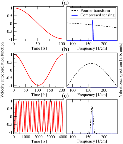
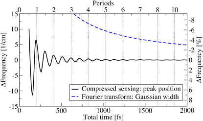
To illustrate the properties of the CS method we start with a simple case, the single vibrational frequency of a diatomic molecule, Na2, that we simulate using ab-initio molecular dynamics. In Fig. 1, we show how the vibrational spectrum depends on the amount of time for which the velocity autocorrelation is calculated. While the discrete FT requires long times to resolve the vibrational frequency, the CS method gives a well-defined peak even with less than one oscillation of the molecular vibrational mode. That the peak is well defined, however, does not imply that peak position is converged. As it can be seen in Fig. 2, the peak position oscillates with the total time until it converges to the proper value after a few periods are sampled. Still, the result converges much faster than compared with the width of the peak given by a FT. We remark that the CS process does not use any additional information about the the signal beyond assuming it is sparse.
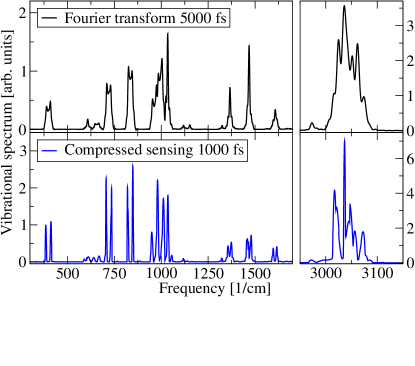
To further demonstrate the advantages of this approach, we now calculate the vibrational spectrum for a benzene molecule from a ab-initio MD simulation, Fig. 3. We can see that the CS approach with 1000 fs obtains a spectrum that is better resolved than the FT results for 5000 fs. This is directly translated into a reduction of the computational time by five times or more. It is reasonable to expect that equivalent gains can be obtained for the computer simulation of other vibrational spectroscopies like infrared and Raman.
IV Optical absorption spectra
Optical absorption is an electronic process. While it can be calculated from a linear response framework Casida (1996); Andrade et al. (2007), it can also be obtained from real-time electron dynamics Yabana and Bertsch (1996). To obtain the spectrum from real-time dynamics the electronic system is propagated under the effect on an electric field of the form . From the propagation the time-dependent dipole moment is obtained, and from the dipole, the frequency-dependent polarizability can be obtained as (atomic units are used in the next two sections)
| (9) |
In order to obtain the full tensor three propagations are required (with in different directions.
The absorption cross-section is related to the trace of the imaginary part of the polarizability tensor
| (10) |
The optical absorption spectra is an ideal candidate for the application of CS. For a molecule, the electronic transitions between bound states produce a discrete spectrum in the low energy region. At higher energies, the transitions to unbound states produce a continuous spectrum. Standard calculation approaches, however, cannot capture this continuous spectrum and approximate it as a sequence of discrete excitations.
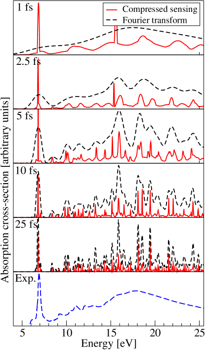
In Fig. 4, we show the optical absorption spectrum for benzene calculated via real-time TDDFT. There we illustrate the effect of the propagation time on the spectrum for CS and FT. From the figure, it is clear that the CS method is capable of resolving the spectrum much better and with a shorter propagation time than a discrete FT. For a given resolution, the FT requires approximately 5 times the propagation time as CS (as can be seen, for example, by comparing the FT at 25 fs with CS at 5 fs).
V Circular dichroism spectra
Another property that can be calculated from real-time electron dynamics is circular dichroism (CD) spectra Yabana and Bertsch (1999); Varsano et al. (2009). A CD spectrum measures the difference in a chiral molecule’s response to left and right circularly-polarized light. The real-time calculation is performed in the same manner as the optical absorption case, but the key quantity to be calculated is now the time-dependent orbital magnetization . The frequency-dependent electric-magnetic cross-response tensor may be obtained as
| (11) |
The rotatory strength, which is the quantity typically plotted in CD spectra, is related to the trace of the imaginary part of according to
| (12) |
The rotatory strength is suitable to the CS scheme because it is sparse in frequency space. In fact, the peaks in a CD spectrum are located at the same positions as in an absorption spectrum. However, the CD spectrum contains both positive and negative peaks.
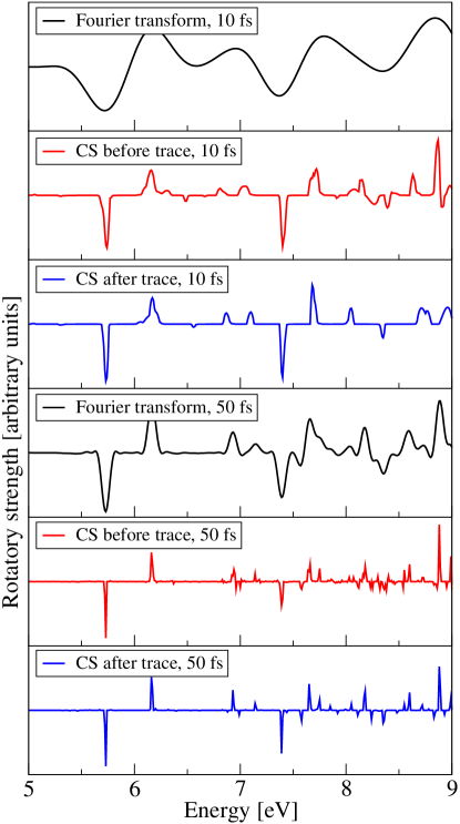
Fig. 5 compares the CD spectrum for (R)-methyloxirane as computed by FT and CS for two different propagation times (10 fs and 50 fs). As can be seen from the figure, for a given propagation time, the CS method provides better spectral resolution than the discrete FT. In fact, just as with linear absorption, FT requires a propagation time approximately 5 times as long as CS to obtain a comparable spectral resolution (as can be seen by comparing the 50 fs FT with the 10 fs CS).
Fig. 5 also illustrates another feature of CS: unlike a direct FT, the CS method is non-linear. Adding together time-resolved signals, then applying CS, generally gives different results from applying CS first and then adding together the results in the frequency domain; this is particularly the case if not all the peaks are well-resolved. In other words, the use of CS to convert time-resolved data into the frequency-domain, as in eq. (11), and the calculation of the trace, as in eq. (12), do not commute. Hence, there are two approaches to obtain the CD spectrum: we can perform CS for each propagation direction and then compute the trace, or we can compute the trace in the time-domain and then perform CS. Both approaches are shown in Fig. 5; at 10 fs, they give similar but not identical results. This is to be expected: the ability of CS to resolve peaks depends on the sparsity of the spectrum. Since each propagation direction is sparser than the sum of all three, CS resolves more peaks at 10 fs when it is performed prior to the trace. For longer propagation times (50 fs), all of the peaks are more fully resolved and the two approaches converge. In any event, both approaches to CS provide much improved resolution over a direct FT for a given propagation time.
VI Numerical methods
Numerically, to find a spectrum using the CS method we need to solve eq. (6). This is not a trivial problem, so we rely on the SPGL1 algorithm developed by van den Berg and Friedlander van den Berg and Friedlander (2008). To avoid numerical stability issues we work with a normalized BPDN problem, where the factors of the matrix, eq. (4), are left out and is normalized. The missing factors are included in after the solution is found. This has the additional advantage of making the noise parameter of eq. (6) dimensionless.
Since we do not a have an a priori estimate for , we do not set it directly. As the SPGL1 algorithm finds a sequence of approximated solutions with a decreasing value of , we set the target value to zero. We assume that the calculation is converged when the value of falls below a certain threshold () or the active space of the system, the set of non-zero coefficients, has not changed for a certain number of iterations (50). In the former case we consider that a solution of the BP problem, eq. (5), has been found. For all the calculations presented here .
CS is much more costly numerically than the discrete FT approach, as it usually involves several hundreds of matrix multiplications. However, this is not a problem for application since usually the solution process normally only takes a few minutes, much less than the computation time required to simulate the real-time dynamics of large atomic systems.
All the calculations presented in this article were performed using the octopus code Castro et al. (2006); Andrade et al. (2012) at the (time-dependent) density functional theory level with the PBE exchange correlation functional Perdew et al. (1996). The adiabatic molecular dynamics calculations were performed from first principles using the modified Ehrenfest method Alonso et al. (2008); Andrade et al. (2009) with a factor of 30 for Na2 and 5 for benzene. The systems were given initial velocities equivalent to 300 K and the MD is performed at constant energy.
All calculations used norm-conserving pseudo-potentials with a real-space grid discretization. The shape of the grid is a union of boxes around each atom. For Na2 we use a spacing of 0.375 a.u. with a sphere radius of 12 a.u., and the MD time-step is 0.057 fs. For benzene, the grid-spacing is 0.35 a.u., the radius is 14 a.u., and the time-step is 0.0085 fs for MD and 0.0017 fs for real-time TDDFT. For (R)-methyloxirane, the spacing is 0.378 a.u., the sphere radius is 15.1 a.u., and the time-step is 0.0008 fs for real-time TDDFT. For the vibrational spectrum calculation we use a time-step 10 times the one of the MD, the energy step is 0.01 1/cm, and the maximum spectrum energy is 5000 1/cm. For the benzene optical absorption spectra, we use a time-step of 0.0017 fs, the energy step is 0.027 eV, and the maximum spectrum energy is 820 eV. For the (R)-methyloxirane circular dichroism spectra, the time-step is 0.0008 fs, the energy step is 0.01 eV, and the maximum spectrum energy is 330 eV. The structure of benzene was taken from ref. Curtiss et al. (1997) and the structure of (R)-methyloxirane was taken from ref. Carnell et al. (1991).
All discrete FTs were performed using third-order polynomial damping: each signal at time was multiplied by prior to Fourier transform, where is the time-length of the signal.
The SPGL1 method used for CS was implemented into octopus based on a Fortran translation of the original Matlab code of van den Berg and Friedlander van den Berg and Friedlander (2007). We plan to release this implementation as a standalone tool in the near future (for the moment the code can be obtained from the octopus repository).
VII Conclusions
We have shown that the CS method can be applied to the numerical calculation of different kinds of atomic and electronic spectra. This results in a significant reduction of the computational time required for the numerical simulations. The effect of this reduction is to increasing the size of the systems that are currently accessible to numerical simulations, and to make possible simulations with more precise, but more costly, methods. It also means that other types of simulations become more affordable from a real-time perspective, for example the combined dynamics of nuclei and electrons that are constrained to short simulation times by the fast dynamics of the electron.
In this work, we have shown the application of CS to the calculation of a few types of spectra, but the method most likely can be applied to other quantities as well, such as non-linear optical response Castro et al. (2004b); Takimoto et al. (2007), magnetic circular dichroism Lee et al. (2011), semi-classical nuclear dynamics Ceotto et al. (2009, 2011), 2D spectroscopy Mančal et al. (2006); Yuen-Zhou and Aspuru-Guzik (2011), etc. Of course, the method is not limited to atomistic simulations and could be applied to simulations in all scientific fields.
The main limitation of the CS approach is that it will not be beneficial for quantities that are not sparse. In such case, the performance of CS will be equivalent to a standard discrete FT. There are some cases where the sparsity requirement might be circumvented. For example, though the real part of the polarizability tensor is not sparse, it could be computed from the imaginary part by using the Kramers-Kronig relation. Another example is crystalline systems Bertsch et al. (2000), where there is a continuum of excitation energies. In this case it might be possible to apply the CS scheme to each -point separately.
We expect that compressed sensing will become widely used in the scientific computing community once its advantageous properties become more widely known. The main difficulty in the adoption of CS is that it is more complex to implement than a discrete FT. This problem can be solved by providing libraries and utilities that can be used by researchers as a black-box. Other issue of the CS approach it has some aspects that might result counter-intuitive at first. For example, non-linearity and the fact that with CS the peak width is not always related to the convergence of the spectrum.
Moreover, we believe that our direct application of the compressed sensing methodology to numerical simulation opens the path for more challenging applications. An idea that we could call “compressed computing”, where the principles of sparsity could be used to design algorithms for numerical simulations that have a reduced computational cost of calculations not only in the number of operations, but also in memory and data transfer bandwidth requirements.
Acknowledgements.
We acknowledge S. Mostame, J. Yuen-Zhou, M.-H. Yung, J. Epstein, M. A. L. Marques, and A. Rubio for useful discussions. The computations in this paper were run on the Odyssey cluster supported by the FAS Science Division Research Computing Group at Harvard University. This work was supported by the Defense Threat Reduction Agency under Contract No HDTRA1-10-1-0046 and by the Defense Advanced Research Projects Agency under award number N66001-10-1-4060. J.N.S. acknowledges support from the Department of Defense (DoD) through the National Defense Science & Engineering Graduate Fellowship (NDSEG) Program. Further, A.A.-G. is grateful for the support of the Camille and Henry Dreyfus Foundation and the Alfred P. Sloan Foundation.References
- Candes et al. (2006) E. Candes, J. Romberg, and T. Tao, IEEE Trans. Inf. Theory 52, 489 (2006).
- Donoho (2006) D. Donoho, IEEE Trans. Inf. Theory 52, 1289 (2006).
- Baraniuk et al. (2010) R. Baraniuk, E. Candes, M. Elad, and Y. Ma, Proc. IEEE 98, 906 (2010), ; and references therein.
- Lustig et al. (2007) M. Lustig, D. Donoho, and J. M. Pauly, Magnet. Reson. Med. 58, 1182 (2007).
- Shabani et al. (2011) A. Shabani, R. L. Kosut, M. Mohseni, H. Rabitz, M. A. Broome, M. P. Almeida, A. Fedrizzi, and A. G. White, Phys. Rev. Lett. 106, 100401 (2011).
- AlQuraishi and McAdams (2011) M. AlQuraishi and H. H. McAdams, P. Natl. Acad. Sci. 108, 14819 (2011).
- Katz et al. (2010) O. Katz, J. M. Levitt, and Y. Silberberg, in Frontiers in Optics (Optical Society of America, 2010) p. FTuE3.
- Rapaport (1995) D. C. Rapaport, The Art of Molecular Dynamics Simulation (Cambridge University Press, 1995).
- Allen and Tildesley (1989) P. Allen and D. Tildesley, Computer Simulation of Liquids, Oxford Science Publications (Clarendon Press, 1989).
- Marx and Hutter (2009) D. Marx and J. Hutter, Ab Initio Molecular Dynamics: Basic Theory and Advanced Methods (Cambridge University Press, 2009).
- Runge and Gross (1984) E. Runge and E. K. U. Gross, Phys. Rev. Lett. 52, 997 (1984).
- Yabana and Bertsch (1996) K. Yabana and G. F. Bertsch, Phys. Rev. B 54, 4484 (1996).
- Castro et al. (2004a) A. Castro, M. A. L. Marques, J. A. Alonso, and A. Rubio, J. Comput. Theor. Nanosci. 1, 231 (2004a).
- Castro et al. (2004b) A. Castro, M. A. L. Marques, J. A. Alonso, G. F. Bertsch, and A. Rubio, Eur. Phys. J. D 28, 211 (2004b).
- Takimoto et al. (2007) Y. Takimoto, F. D. Vila, and J. J. Rehr, J. Chem. Phys. 127, 154114 (2007).
- Andrade et al. (2012) X. Andrade, J. Alberdi-Rodriguez, D. A. Strubbe, M. J. Oliveira, F. Nogueira, A. Castro, J. Muguerza, A. Arruabarrena, S. G. Louie, A. Aspuru-Guzik, A. Rubio, and M. A. L. Marques, J. Phys.: Condens. Matter 24, 233202 (2012).
- Baraniuk (2007) R. Baraniuk, IEEE Signal Process. Mag. 24, 118 (2007).
- Candes and Wakin (2008) E. Candes and M. Wakin, IEEE Signal Process. Mag. 25, 21 (2008).
- Chartrand et al. (2010) R. Chartrand, R. G. Baraniuk, Y. C. Eldar, M. A. T. Figueiredo, and J. Tanner, IEEE J. Sel. Topics Signal Process. 4, 241 (2010).
- Dickey and Paskin (1969) J. M. Dickey and A. Paskin, Phys. Rev. 188, 1407 (1969).
- Casida (1996) M. Casida, in Recent Developments and Applications of Modern Density Functional Theory, edited by J. Seminario (Elsevier Science, Amsterdam, 1996) p. 391.
- Andrade et al. (2007) X. Andrade, S. Botti, M. A. L. Marques, and A. Rubio, J. Chem. Phys. 126, 184106 (2007).
- Koch and Otto (1972) E. Koch and A. Otto, Chem. Phys. Lett. 12, 476 (1972).
- Yabana and Bertsch (1999) K. Yabana and G. F. Bertsch, Phys. Rev. A 60, 1271 (1999).
- Varsano et al. (2009) D. Varsano, L. E. Leal, X. Andrade, M. Marques, R. di Felice, and A. Rubio, Phys. Chem. Chem. Phys. 11, 4481 (2009).
- van den Berg and Friedlander (2008) E. van den Berg and M. P. Friedlander, SIAM J. Sci. Comput. 31, 890 (2008).
- Castro et al. (2006) A. Castro, H. Appel, M. Oliveira, C. A. Rozzi, X. Andrade, F. Lorenzen, M. A. L. Marques, E. K. U. Gross, and A. Rubio, Phys. Status Solidi B 243, 2465 (2006).
- Perdew et al. (1996) J. P. Perdew, K. Burke, and M. Ernzerhof, Phys. Rev. Lett. 77, 3865 (1996).
- Alonso et al. (2008) J. L. Alonso, X. Andrade, P. Echenique, F. Falceto, D. Prada-Gracia, and A. Rubio, Phys. Rev. Lett. 101, 096403 (2008).
- Andrade et al. (2009) X. Andrade, A. Castro, D. Zueco, J. L. Alonso, P. Echenique, F. Falceto, and A. Rubio, J. Chem. Theo. Comput. 5, 728 (2009).
- Curtiss et al. (1997) L. A. Curtiss, K. Raghavachari, P. C. Redfern, and J. A. Pople, J. Chem. Phys. 106, 1063 (1997), geometries downloaded from http://tinyurl.com/3zb5xxk.
- Carnell et al. (1991) M. Carnell, S. Peyerimhoff, A. Breest, K. Gödderz, P. Ochmann, and J. Hormes, Chem. Phys. Lett. 180, 477 (1991).
- van den Berg and Friedlander (2007) E. van den Berg and M. P. Friedlander, “SPGL1: A solver for large-scale sparse reconstruction,” (2007), http://www.cs.ubc.ca/labs/scl/spgl1.
- Lee et al. (2011) K.-M. Lee, K. Yabana, and G. F. Bertsch, J. Chem. Phys. 134, 144106 (2011).
- Ceotto et al. (2009) M. Ceotto, S. Atahan, G. F. Tantardini, and A. Aspuru-Guzik, J. Chem. Phys. 130, 234113 (2009).
- Ceotto et al. (2011) M. Ceotto, S. Valleau, G. F. Tantardini, and A. Aspuru-Guzik, J. Chem. Phys. 134, 234103 (2011).
- Mančal et al. (2006) T. Mančal, A. V. Pisliakov, and G. R. Fleming, J. Chem. Phys. 124, 234504 (2006).
- Yuen-Zhou and Aspuru-Guzik (2011) J. Yuen-Zhou and A. Aspuru-Guzik, J. Chem. Phys. 134, 134505 (2011).
- Bertsch et al. (2000) G. Bertsch, J.-I. Iwata, A. Rubio, and K. Yabana, Phys. Rev. B 62, 7998 (2000).