Superfluid to normal phase transition in strongly correlated bosons in
two
and three dimensions
Abstract
Using quantum Monte Carlo simulations, we investigate the finite-temperature phase diagram of hard-core bosons ( model) in two- and three-dimensional lattices. To determine the phase boundaries, we perform a finite-size-scaling analysis of the condensate fraction and/or the superfluid stiffness. We then discuss how these phase diagrams can be measured in experiments with trapped ultracold gases, where the systems are inhomogeneous. For that, we introduce a method based on the measurement of the zero-momentum occupation, which is adequate for experiments dealing with both homogeneous and trapped systems, and compare it with previously proposed approaches.
pacs:
64.60.-i, 67.85.-d, 03.75.Hh, 02.70.SsI Introduction
The description of strongly correlated bosonic systems is of fundamental interest in largely diverse physical situations ranging from low-temperature experiments with superfluid helium Daunt and Smith (1954) to Josephson-junction arrays Brutel et al. (1993), as well as magnetic insulators giamarchi et al. (2008) and ultracold gases in optical lattices Bloch et al. (2008); cazalilla_review_11 . The latter systems offer an unparalleled playground to study fundamental models widely considered in statistical and condensed-matter physics. This is because of the high degree of control over the experimental parameters that determine the Hamiltonian describing the system. In particular, the Bose-Hubbard model Fisher et al. (1989); Jaksch et al. (1998) has been experimentally realized in one Stöferle et al. (2004), two Spielman et al. (2007); Jimenez-Garcia et al. (2010), and three dimensions Greiner et al. (2002), where the superfluid to Mott-insulator transition has been observed. Even though it has received less attention, the superfluid to normal transition in the Bose-Hubbard model has been investigated experimentally in three dimensions Trotzky et al. (2010), while in two dimensions it has been realized in the form of a two-dimensional lattice of Josephson-coupled Bose-Einstein condensates Schweikhard et al. (2007); Trombettoni, Smerzi, and Sodano (2005), as well as in experiments with ultracold atoms in optical lattices zhang_chin_12 .
Although experiments with ultracold atoms on optical lattices are in some respects almost ideal realizations of model Hamiltonians of interest, significant complications arise because of the presence of a confining potential, which leads to the coexistence of different phases in a single experimental setup Batrouni et al. (2002); rigol_09 . Furthermore, the mesoscopic size of the system in combination with the inhomogeneity induced by the trapping potential produces a rounding off of the otherwise sharp features present in an infinite homogeneous system in the critical region rigol_03 ; wessel_04 ; campostrini_vicari_10a ; campostrini_vicari_10b . Thus the understanding and assessment of criticality in such systems remains a challenging task.
The emergence of sharp features in the momentum distribution as obtained from time-of-flight images has been frequently associated to the emergence of superfluidity Greiner et al. (2002); Chin et al. (2006); Xu et al. (2006); Tung et al. (2010); clade et al. (2009). However, this association may not be accurate because sharp peaks in the momentum distribution already appear in the normal state, due to an increasing correlation length when approaching a critical regime Kashurnikov et al. (2002); Diener et al. (2007); Kato et al. (2008). More recently, new schemes to detect criticality in trapped systems have been proposed. In some of those studies, a detailed analysis of the momentum distribution was used to define criteria that allow one to extract reliable estimations of the critical points from time-of-flight images Diener et al. (2007); Trotzky et al. (2010); Pollet et al. (2010). In addition to time-of-flight images, high-resolution in situ imaging of the density profile of trapped systems has become a powerful instrument with which one can also study phase diagrams of strongly correlated systems and quantum criticality. Numerous theoretical and experimental studies based on this idea have been carried out for systems in the presence of an optical lattice Fölling et al. (2006); Zhou et al. (2009); Gemelke et al. (2009); Ho and Zhou (2010); Nascimbene, Navon, Chevy, and Salomon (2010); Ma, Pollet and Troyer (2010); Bakr et al. (2010); Sherson et al. (2010); Zhang, Hung, Tung, Gemelke, Chin (2011); Fang, Chung, Ma, Chen, and Wang ; Hazzard and Mueller (2011) and in the absence of it Kruger et al. (2007); Nascimbene et al. (2010); Hung et al. (2011); duchon_trivedi_11 .
One important aspect that determines the nature of the quantum phases and their associated order parameters is the dimensionality . Mermin et al. rigorously proved that at any nonzero temperature, continuous symmetries cannot be spontaneously broken in systems with sufficiently short-range interactions in dimensions Mermin and Wagner (1966); Hohenberg (1967). This implies that, at finite temperature, Bose-Einstein condensation (BEC) cannot occur in one and two dimensions. Two-dimensional Bose systems, however, are marginal in the sense that fluctuations are strong enough to destroy the fully ordered state but are not so strong as to suppress superfluidity. Thus critical behavior develops in the Berezinskii-Kosterlitz-Thouless (BKT) transition berezinskii_72 ; kosterlitz_thouless_73 , where a superfluid phase with quasi-long-range order competes with thermal fluctuations and induces a continuous phase transition to the normal fluid as the temperature is increased. In addition to low-temperature superfluidity, long-range order can develop at zero temperature in two dimensions. On the other hand, in three dimensions, the superfluid transition is accompanied by the appearance of true long-range order, implying that the system also exhibits Bose-Einstein condensation. Such a transition, which belongs to the three-dimensional universality class, is well understood in the sense that the critical exponents have been determined experimentally and theoretically with remarkably high accuracy in many different physical contexts Li and Teitel (1989); Salamon, Shi, Overend, and Howson (1993); Overend, Howson, and Lawrie (1994); Campostrini et al. (2001); campostrini_vicari_06 ; burovski_svistunov_06 ; hasenbusch_torok_99 .
Here, we focus our study on the superfluid to normal transition in a system of strongly interacting bosons in two- and three-dimensional lattices. Specifically, we consider the Bose-Hubbard model in the limit of infinite on-site repulsion, i.e., the hard-core boson limit. We use exact quantum Monte Carlo simulations to compute the finite-temperature phase diagram as a function of chemical potential. Accurate results are obtained through finite-size scaling of the condensate fraction and/or the superfluid stiffness obtained from our simulations. We also determine the mean-field phase diagram, which is qualitatively correct but quantitatively quite different from the exact results. We then proceed to study the superfluid to normal phase transition in two and three dimensions in the presence of a confining potential, which is required to describe experiments with ultracold gases. We introduce a method to determine the critical temperature, for any given density, that is based on the measurement of the zero-momentum occupation as a function of temperature. This method is in principle adequate for experiments dealing with both homogeneous and trapped systems. Furthermore, we compare our approach to other recently proposed schemes based on the in situ density images Zhou et al. (2009) as well as on the shape of the low-momentum part of the momentum distribution Pollet et al. (2010).
The paper is organized as follows. In Sec. II, we introduce the model and its phase diagram in two and three dimensions supplemented with the mean-field calculations. Section III is devoted to the discussion of the techniques to obtain the phase boundaries. In Sec. IV, we discuss the possibility to have Bose-Einstein condensation in trapped two-dimensional systems as well as the methods to determine the phase boundaries from experimentally accessible quantities. Finally, in Sec. V, we draw our conclusions.
II Model and phase diagram
We consider a system of hard-core bosons on a -dimensional lattice with sites. The Hamiltonian can be written as
| (1) |
where () is the boson creation (annihilation) operator at a given site , and is the local particle number operator. The hard-core boson creation and annihilation operators satisfy the constraint , which forbids multiple occupancy of lattice sites. The first term in Eq. (1) is the kinetic energy, where is the hopping amplitude between neighboring sites and (). In experiments involving ultracold gases, a trap is required to confine the atoms. The effect is taken into account in the second term that contains , where is its strength and is the overall chemical potential. is the distance from site to the center of the trap. In what follows, positions will be given in units of the lattice spacing and the energy will be given in units of the hopping amplitude .
We recall that the Hamiltonian in Eq. (1) can be exactly mapped to the extensively studied quantum model matsubara_matsuda_56
| (2) |
where is the th component of the spin- spin operator at site . In the spin language, the term proportional to describes a ferromagnetic exchange interaction, while the one proportional to describes a magnetic field in the -direction at site .
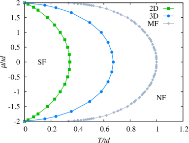
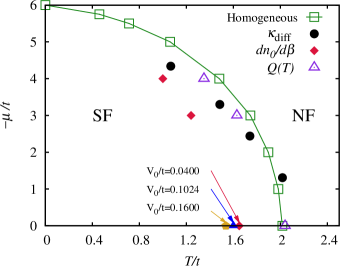
We study the Hamiltonian in Eq. (1), at finite temperature , by means of the stochastic series expansion (SSE) quantum Monte Carlo (QMC) method with operator-loop updates Sandvik and Kurkijarvi (1991); sandvik_92 ; Dorneich and Troyer (2001). The determination of the phase diagrams is carried out through a finite size scaling of the condensate fraction and/or the superfluid stiffness using periodic boundary conditions. The numerically exact (QMC) phase diagram in two dimensions (2D) and three dimensions, as well as the the mean-field predictions, are presented in Fig. 1. The finite-temperature phase diagram comprises an off-diagonal long-range-ordered (ODLRO) low-temperature superfluid lobe (quasi-ODLRO in 2D) surrounded by a high-temperature normal phase with exponentially decaying correlation functions. The extend of the superfluid state is expected to be hindered as dimensionality is reduced because thermal and quantum fluctuations have a stronger effect in low-dimensional systems. Clearly, our results agree with that expectation. The dissimilarity between the mean-field and the exact phase diagrams makes it clear that both thermal and quantum fluctuations are strong and play an important role even in three dimensions, where mean-field approaches are generally considered to be a good approximation.
Details on the procedure to obtain the phase boundaries are provided in the following sections. Such procedures are different in two and three dimensions because of the different universality class of the phase transition.
III Homogeneous systems
III.1 Two dimensions
Our results for the two-dimensional phase diagram in Fig. 1 are based on the fact that the model in Eq. (1) undergoes a BKT transition as a function of the temperature. This phase transition has been studied in great detail the context of the two-dimensional quantum model in Eq. (2) in the absence of a magnetic field loh_grant_85 ; ding_makivic_90 ; ding_92 ; harada_kawashima_97 . Kosterlitz and Thouless predicted that the superfluid stiffness jumps from zero to the value at the critical temperature. Thus we consider measurements of the superfluid stiffness for different system sizes as a function of temperature. Within the SSE method, the superfluid stiffness is computed by measuring the fluctuation of the winding number pollock_ceperley_87 ; they are connected through the relation , where is the inverse temperature.
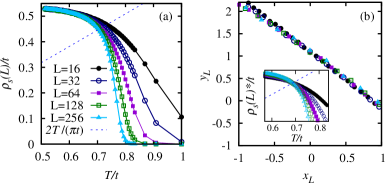
Figure 2(a) shows results for the superfluid stiffness of 2D hard-core bosons at [or, equivalently, the spin stiffness of the 2D model in Eq. (2)] as a function of for several system sizes. The observed slow approach of the superfluid stiffness to the characteristic jump expected for the infinite system is due to strong finite-size effects at the BKT transition. Finite-size scaling relations for the superfluid stiffness can be derived by integrating the Kosterlitz renormalization-group equations (see, for instance, Refs. harada_kawashima_97, ,olsson_95, ,weber_minhagen_88, ). This procedure yields
| (3) |
where measures the distance from the critical point and depends only weakly on temperature. Close to the critical point, . In the limit , a scaling form for the superfluid stiffness based on Eq. (3) can be written as
| (4) |
From Eq. (3) in the limit , . From Eq. (4), one can find the scaling function and critical temperature by computing and based on our Monte Carlo simulations for different and . The adjustment of the constant and critical temperature , such that the data produce the best possible collapse, yields a numerical estimate of the scaling function and the critical temperature itself. The result of the determination of the scaling function is reported in Fig. 2(b), where a plot of as a function of is presented. Notice that as expected, the value of is very close to one for . Furthermore, one expects from Eq. (3) that a plot of the rescaled superfluid stiffness as a function of the temperature should become system-size independent at the critical temperature . This observation is confirmed in the inset of Fig. 2(b). Remarkably, those curves intersect with the line right at the critical temperature, in agreement with the BKT scenario. Our result is consistent with the best value reported in Ref. harada_kawashima_97, , for which note:better . An analogous procedure to the one just described is carried out for different values of the chemical potential to complete the two-dimensional phase diagram in Fig. 1. We should mention that Eq. (3) predicts the value of the superfluid stiffness in an infinite system at the critical temperature to be . However, in Ref. hasenbusch_05, , it was shown that the superfluid stiffness at the transition temperature is , which is very close to the result based on Eq. (3) (). Detecting the difference is beyond the accuracy of the present study.
III.1.1 Critical value from
We now briefly discuss the behavior of the occupation of the zero momentum state () in the critical region and address the determination of the transition temperature from it. In a homogeneous and infinite 3D system, BEC is identified by a macroscopic occupation of . However, as mentioned before, thermal fluctuations in 2D destroy Bose-Einstein condensation. Nonetheless, as the superfluid transition is approached from the normal phase, diverges [see inset in Fig. 3(a)]. Indeed, from the Fourier transform of the one-body density matrix in the long-distance limit , one can extract the behavior of as is approached,
| (5) |
We assume the essential singularity of the correlation length , where is a chemical-potential-dependent scaling factor. From Eq. (5), it follows that not only does diverge at , but also its derivative with respect to ,
| (6) |
In a finite system, when is close to , the role of the correlation length is taken over by when . This occurs at a characteristic temperature given by
| (7) |
where is a nonuniversal factor related to . At that temperature, the derivative in Eq. (6) scales with the system size as
| (8) |
Below , cannot vary as fast as right above because the exponential increase of the correlation length is truncated by . Below , the variation of comes mainly from the temperature dependence of the anomalous exponent, which is not as strong as the variation due to the exponential behavior of the correlation length. Consequently, should exhibit a sharp minimum at the size-dependent temperature . Moreover, in a finite system, cannot grow indefinitely as the temperature is lowered. With decreasing temperature (), must approach its (finite) value, which implies that .
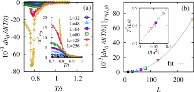
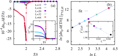
Figure 3(a) depicts the derivative of the for different system sizes vs . The divergence of is apparent. A sharp minimum develops and its location approaches as the system size increases. This is expected from the finite-size relation in Eq. (7). The scaling of the height of this minimum is studied in Fig. 3(b), where we plot the absolute value of vs . The data follows the scaling relation in Eq. (8), as made evident by a fit to the function . In the inset in Fig. 3(b), we show the finite-size scaling of . We observe that is consistent with the scaling relation in Eq. (7), which we use to obtain the critical temperature in the thermodynamic limit. We find . This value is compatible with the one found by performing the finite-size scaling of the superfluid stiffness. While this approach is obviously less accurate than the one discussed before for , among other things because a numerical derivative is involved, the fact that it works extremely well is very important for current trapped ultracold gas experiments where the superfluid density cannot be measured.
We note at this point that in the determination of Eq. (8), we have neglected multiplicative logarithmic corrections that affect the behavior of the zero-momentum occupation and thus its derivative with respect to the temperature amit_grinstein_80 ; kenna_irving_95 . In fact, the exponent of the logarithm in Eq. (8) gets modified to
| (9) |
with (Ref. kenna_irving_95, ). However, this correction does not affect the determination of the critical temperature, which is based on the location of the position of the peak in the numerical derivative and the scaling relation in Eq. (7). Furthermore, the correction to the exponent of the logarithm is very small and, at least within the precision of our simulations, its effect is hardly detectable.
III.2 Three dimensions
In order to determine the 3D phase diagram, we follow the same procedure as in 2D. In 3D, however, the superfluid to normal transition belongs to the 3D universality class. This transition, for the model in Eq. (1), has also been studied using QMC simulations in the past. for BEC was evaluated as a function of the density in Ref. pedersen_schneider_96, . The onset of magnetization as a function of the magnetic field (or, in the bosonic language, the density as a function of the chemical potential) was investigated in Ref. kawashima_04, . Furthermore, the fate of the superfluid phase under the effect of an additional ring-exchange term was studied in Ref. melko_scalapino_05, . Here, we determine the full phase diagram (shown in Fig. 1) as a function of the temperature and the chemical potential. We begin by considering measurements of the superfluid stiffness. In dimensions, as the critical temperature is approached, the superfluid stiffness vanishes continuously as fisher_jasnow_73
| (10) |
where the exponent determines how the correlation length diverges when approaching the critical temperature, i.e.,
| (11) |
As a result, at the critical temperature, the superfluid stiffness scales with the linear size of the system as . This, in turn, allows one to write the scaling hypothesis for the superfluid stiffness as a function of the system size and the temperature as
| (12) |
which we utilize to determine the critical temperature. In Fig. 4(a), we show results for the superfluid stiffness in a 3D lattice vs for different system sizes.

We numerically extract the scaling function by studying the rescaled superfluid stiffness [left-hand side in Eq. (12)] vs the rescaled temperature . Classical Monte Carlo simulations yield the correlation length exponent campostrini_vicari_06 , and burovski_svistunov_06 , which we use to produce the collapse presented in Fig. 4(b). With at hand, it is enough to fix such that the best collapse of the data is achieved. Furthermore, the inset shows the rescaled superfluid stiffness as a function of temperature, which becomes system-size independent at the critical temperature, as implied by the scaling hypothesis in Eq. (12). Our best estimation of the critical temperature for is (to be compared with from Ref. pedersen_schneider_96, and more recently with from Ref. laflorencie_12, ). We perform a similar analysis for different values of the chemical potential to complete the three-dimensional phase diagram in Fig. 1.
Additionally, since the superfluid to normal phase transition in our model in 3D is accompanied by the emergence of true long-range order, one can study the transition by computing the condensate fraction associated with the appearance of BEC. Following Penrose and Onsager penrose56 , the condensate fraction is defined as the ratio of the largest eigenvalue of the one-body density matrix to the total number of particles . For the system under consideration, condensation occurs to the zero-momentum state due to translational invariance, thus the condensate fraction is . The behavior of can be obtained from the Fourier transform of the one-body density matrix in the long-distance limit, which in 3D is given by
| (13) |
Here, is the correlation function exponent, also known as the anomalous scaling dimension. On approach to , diverges with the correlation length as Pollet et al. (2010)
| (14) |
In a finite system, this relation implies that the condensate fraction vanishes at the critical point as , which we adopt to formulate the following scaling hypothesis for the condensate fraction
| (15) |
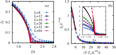
In the determination of through the scaling relation in Eq. (15), we use the value campostrini_vicari_06 . The results are summarized in Fig. 5, where a plot of the condensate fraction vs is shown in panel (a). In Fig. 5(b), the data collapse of the rescaled condensate fraction vs the rescaled temperature is apparent. Furthermore, in the inset, one can observe that curves of the rescaled condensate fraction vs become system-size independent at , as implied in Eq. (15). This procedure results in a for , which is in remarkably good agreement with our previous estimate using the superfluid stiffness.
III.2.1 Critical value from
Similarly to the 2D case, diverges in the vicinity of the superfluid to normal phase transition. It diverges with the correlation length as
| (16) |
Also, as in 2D, in a finite 3D system at a temperature close to , the role of the correlation length is taken over by when . The characteristic temperature is given by
| (17) |
where is a non-universal factor. At , scales with the system size as
| (18) |
Furthermore, in a finite system, reaches its minimum value at because the divergence of the correlation length can no longer be sustained. This is expected from the behavior of vs , shown in the inset in Fig. 6(a), where is first seen to increase as the temperature is lowered and then to saturate as . The changes observed in that low temperature regime originate in the smooth dependence of the correlation function exponent on the temperature, as opposed to the fast change produced by the strong divergence of the correlation length. Hence, once again, exhibits a sharp minimum at the size-dependent temperature in Eq. (17) and then goes to zero.
In Fig. 6(a), we display results for vs for different system sizes. The divergence in the derivative, anticipated by Eqs. (16) and (18), is confirmed by the presence of sharp minima that grow with system size. The finite-size scaling of the height of the sharp minimum in Eq. (18) is presented in Fig. 6(b), where we plot the logarithm of the maximum height of vs . According to Eq. (18), such a plot should turn into a straight line with a slope given by . A fit of our data to the function , yields . The scaling relation given by Eq. (18) is thus confirmed as our value of is compatible with the exponents from Ref. campostrini_vicari_06, , which yield . The size dependence of the position of the peaks anticipated in Eq. (17) is verified in the inset of Fig. 6(b). Within this procedure, we find that the critical temperature in the thermodynamic limit is , which is in relatively good agreement with the one obtained through the finite-size scaling of both the superfluid stiffness and the condensate fraction.
We conclude this section by mentioning that in determining the critical temperature, we have used the leading scaling forms and subleading corrections to scaling have been neglected. For the 3D universality class, such corrections have been reviewed in Ref. pelissetto_vicari_02, . We note that in our calculations, there is an excellent collapse of the data, which suggests that the effects of the subleading corrections to scaling are small. Furthermore, the most accurate results obtained for follow from completely independent measurements, i.e., the superfluid and condensate fractions. They agree within the error bars, which further supports the relevance of the scaling relations used.
III.3 Mean field
To gain an understanding of the effects of quantum fluctuations in our systems, we have also calculated the mean-field phase diagram for this model. We utilize the standard decoupling of the kinetic energy term in the Hamiltonian in Eq. (1) Sheshadri (1993)
| (19) |
where is the condensate order parameter, to be determined self-consistently. The angle brackets denote the usual thermal average. The above mean-field decoupling allows one to write a mean-field Hamiltonian for Eq. (1) as
| (20) |
For homogeneous systems, i.e., , Eq. (20) can be recast in the following manner,
| (21) |
where is the mean-field Hamiltonian per lattice site. Note that in this case the superfluid order parameter can be taken to be real. The corresponding partition function at finite inverse temperature is
| (22) |
A self-consistency condition for the superfluid order parameter can be derived by noting that
| (23) |
Using the relation (23), we arrive at the equation that determines the order parameter ,
| (24) |
which is valid whenever . We solve Eq. (24) numerically and determine the superfluid region, , as a function of the temperature and the chemical potential. The phase boundaries are determined as the values of and for which . For , Eq. (24) reduces to
| (25) |
which is the equation that determines the mean-field magnetization of the Ising model in the absence of a magnetic field. The critical temperature is, of course , which is quite different from the results of our quantum Monte Carlo simulations in two and three dimensions.
IV Trapped systems
In experiments involving ultracold atoms, an additional trapping potential is necessary to contain the gas. While a qualitative (and sometimes a reasonably good quantitative) description of the trapped system can be obtained within the local density approximation (LDA) from the properties of the homogeneous system, this approximation may breakdown in regimes of interest. In particular, the latter occurs at criticality, where the correlation length diverges and deviations from the LDA description can be large Pollet et al. (2010). Furthermore, as we explain below, in trapped 2D systems care needs to be taken with the application of the Mermin-Wagner-Hohenberg theorem. Therefore, we focus our attention on those two aspects, namely, the possibility to have BEC the in the presence of an additional external confining potential in 2D, and the study of criticality in 2D and 3D.
IV.1 Absence of BEC in interacting 2D systems
We mentioned in the Sec. I that homogeneous 2D systems are special because thermal fluctuations destroy any order at finite temperature. However, harmonically confined non-interacting bosons can undergo BEC at finite temperature Dalfovo et al. (1999). In this case, the arguments by Mermin et al. are not violated because condensation does not occur to the zero-momentum state, but to a single-particle eigenstate of the trapped system. One can then wonder whether finite-temperature BEC persists in the presence of interactions. By following analogous arguments to those in Ref. mullin_97, , we show below that interactions do preclude the formation of a condensate in the Bose-Hubbard model in the presence of the trap. This is so because there is a close connection between the formation of a condensate and the macroscopic population of the zero-momentum occupation, which is forbidden in 2D at finite temperature.
Generally speaking, the emergence of BEC is established through the evaluation of the condensate fraction , which is defined as the ratio of the largest eigenvalue of the one-body density matrix to the total number of particles ,
| (26) |
If after taking the appropriate thermodynamic limit remains finite, then the system exhibits BEC. Otherwise, if it becomes zero, there is no condensation penrose56 .
Alternative forms of the criteria expressed through Eq. (26) can be useful when the system is not spatially uniform; they are based on the following inequality penrose56 :
| (27) |
where are the eigenvalues of the one-body density matrix . We define the quantity
| (28) |
which is just a lattice version of its analogous quantity defined on the continuum in Ref. penrose56, . It follows from Eqs. (27) and (28) that
| (29) |
Therefore, if remains finite in the thermodynamic limit, then the system exhibits BEC. A further criterion can be defined and it depends on the quantity
| (30) |
Notice that is the square of the mean value of the function , while is the mean value of . Since the variance of the function is either positive or zero, it follows that
| (31) |
Now, since is a positive-semidefinite Hermitian matrix, its elements satisfy penrose56 ; horn (2000)
| (32) |
where is an upper bound of the local density . By summing over and in Eq. (32) and the square of it, we find a lower bound for ,
| (33) |
As long as the local density remains finite throughout the whole system, can be taken to be finite and independent of . This, in turn, implies that if , then BEC takes place; otherwise if , then no BEC occurs penrose56 . Notice that if , then coincides with the ratio of the zero-momentum occupation to the total number of particles, i.e., the fraction of particles in the system that condenses to the zero-momentum state. Since in two dimensions vanishes because of the Mermin et al. theorem, then is zero too. In the specific case of the Bose-Hubbard model in the presence of an inhomogeneous potential in thermal equilibrium, we have that . Furthermore, the density is finite everywhere across the system because of the on-site interaction, implying that .
Hence, even in the presence of the trap, there is no condensation in the 2D Bose-Hubbard model at finite . Note that this argument does not preclude condensation in the non-interacting limit, where the density can diverge at the minimum of the inhomogeneous potential in the thermodynamic limit and BEC can indeed occur to the lowest single-particle eigenstate, but not to the zero-momentum state. Moreover, the criteria above implies that for the Bose-Hubbard model in in thermal equilibrium, condensation to any state has to be accompanied by condensation to the zero-momentum state.
In our proof, we have stated that for the Bose-Hubbard model in thermal equilibrium holds. We now present two independent arguments for why . The first one is based on the fact that the matrix elements of the von Neumann’s statistical operator in the position representation are strictly positive campbell_senger_84 . Since the one-body density matrix corresponds to a partial trace of the von Neumann’s statistical operator penrose56 . it follows that its elements are positive too. A rather technical, but yet rigorous, argument is based on the series expansion representation of the one-body density matrix that we used in our Monte Carlo implementation. Within this representation, the measurements of the one-body density matrix are based on the extension of the configuration space where these off-diagonal quantities are well defined Dorneich and Troyer (2001). In such extended space, the one-body density matrix is represented as the sum of strictly positive matrix elements (hence ) which are, in turn, efficiently sampled during the construction of the loop operators in the directed-loop update algorithm alet_troyer_05 .
IV.2 Two dimensions
IV.2.1 Local compressibility
Exactly as in the homogeneous system, even though there is no condensation in 2D, a superfluid phase is expected in the trapped system at low temperatures. Because of the inhomogeneity introduced by the confining potential, the coexistence of space separated normal and superfluid domains can occur at intermediate temperature. In that case, there must be a region in the trap where superfluidlike domains transition into normal ones. Within the LDA, this region is such that the local chemical potential coincides with the critical of the bulk system for the normal-to-superfluid phase transition.
Based on this idea, Zhou and collaborators proposed a method to identify the phase boundaries of the homogeneous system from a high-resolution scan of the local density across the confined system Zhou et al. (2009). This method requires the determination of the local compressibility defined as
| (34) |
and relies on the expectation that the local density profile , as well as the local compressibility , can be well approximated by their bulk values through the LDA. The existence of sharp features in the local compressibility at specific locations in the trap is then associated with phase transitions occurring in the homogeneous system as a function of the chemical potential. This method is expected to be accurate in the limit of very shallow traps where the contribution from density gradients due to the trapping potential are small Zhou et al. (2010).

In Fig. 7, we present QMC results for the density profile of a 2D trapped system, as well as the local compressibility, as a function of the distance from the center of the trap. The expected sharp features in the local compressibility due to critical fluctuations are smoothed by finite-size effects. They are replaced by a rounded maximum, which can be associated with the superfluid to normal transition Zhou et al. (2010). The location of the maximum is connected to the critical chemical potential through . For the case in Fig. 7, we get . This value is to be contrasted with , which we obtained in the homogeneous system calculations. As increases, however, the agreement between the estimates of the critical chemical potential based on the local compressibility and the results of the homogeneous system worsens. For instance, for , we find that , as opposed to the homogeneous system result where . This occurs presumably because, closer to the tip of the superfluid lobe, critical fluctuations are stronger, and thus larger violations of the LDA are expected.
IV.2.2 Momentum distribution function
Another quantity that can be measured in experiments with ultracold atoms is the momentum distribution function. At fixed chemical potential (), when lowering , the normal-to-superfluid crossover in the trapped system proceeds via the creation and growth of a superfluid domain in the center of the trap. (The rate of growth of the superfluid domain will depend on the functional form and strength of the confining potential.) Hence, the zero-momentum state becomes increasingly populated. As follows from the discussion for finite homogeneous systems, it is expected that as decreases and approaches for the normal-to-superfluid transition in the center of the trap, the rate of growth of will increase. Below , on the other hand, will eventually decrease because of the finite extend of the system imposed by the confining potential. If is lowered well below , then almost the entire system will become superfluid and the observables will saturate their (finite) zero-temperature values.
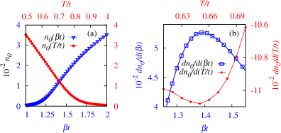
Hence, just as in the homogeneous case, one can attempt to estimate for the superfluid to normal phase transition for the density in the center of the trap by measuring the temperature at which the rate of change of is extremal. This approach provides an accurate estimate for the homogeneous system and it is expected to be accurate in confined systems with shallow trapping potentials. Figure 8(a) depicts the evolution of vs as well as the inverse temperature of a harmonically confined 2D system with () and in the center of the trap. In Fig. 8(b), we show which, as expected, exhibits a minimum located at . This temperature is compatible with the value of obtained for the homogeneous case where, after a finite-size scaling, we obtained . Our estimate derived from the study of a single trapped system is about off the value of the homogeneous system.
One can perform the same analysis based on measurements of , but now as a function of the inverse temperature . In that case, one expects a maximum in the derivative instead of a minimum. In general, for finite and not very large systems, the position of such maximum will not coincide with obtained from the minimum of . Overall, we find that for the system sizes available to our QMC simulations, the analysis based on provides more accurate estimates of the critical temperature than the one based on . Furthermore, the maximum found in is consistently sharper and better defined with respect to the minimum found for which instead is shallower and broader, and thus harder to detect and numerically less reliable.
Based on measurements of presented in Fig. 8(b) on the same system with (), , we find , which is also very close to the critical temperature of the homogeneous system. When the maximum is sharply defined, in the limit of very shallow traps with large numbers of bosons, the two approaches are expected to coincide (i.e., their difference is due to finite-size effects). As a matter of fact, for the homogeneous 2D and 3D systems in Sec. III, where the minima of are sharp, we find that the analysis using and yields essentially the same results for . In the Appendix, we provide an analytic understanding of this in terms of a simple function. Therefore, for the determination of the phase diagram based on measurements in harmonically confined systems, we consider only measurements based on .
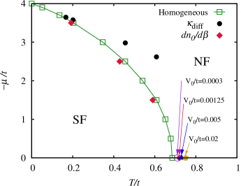
In Fig. 9, we summarize our results for the determination of the critical parameters with the local compressibility as well as with the derivative of the zero-momentum occupation with respect to , and contrast them with the phase diagram of the homogeneous system. Clearly, all methods work well for large values of and small values of (equivalent to approaching the continuum limit in a lattice system). Close to the tip of the superfluid region, the method based on performs much better than the one based on .
At the tip of the superfluid lobe, where the size effects are expected to be the strongest, we observe that as the size of the system is increased (or the strength of the trap is decreased), keeping constant the chemical potential in the center of the trap, the estimate of the critical temperature decreases approaching the result in homogeneous systems.
IV.3 Three dimensions
We now turn our attention to the study of criticality in 3D trapped systems. We make use of the same ideas developed for 2D system to extract the critical parameters, i.e., measurements based on the zero-momentum occupation as well as on the local compressibility.
Additionally, in 3D, we can utilize a method that is based on the analysis of the shape of the central peak for the momentum distribution. With it, one can construct a quantity that exhibits a minimum at the critical point Pollet et al. (2010). The idea behind this method is that close to criticality, the momentum distribution develops a bimodal structure whose evolution as a function of temperature contains information about the formation of a superfluid region in the center of the trap. At , when a superfluid domain begins to form, the major contribution to the occupation of the zero-momentum state comes from regions that are not critical, i.e., from regions that are far away from the center of the trap. However, the derivatives of the momentum distribution are critical, in the sense that they can be understood in terms of an LDA integral that diverges at the center of the trap, where the system is critical. Based on that idea, the following quantity was devised in order to extract the critical temperature Pollet et al. (2010):
| (35) |
where is the momentum at which is maximum and the exponent . In Ref. Pollet et al., 2010, it was shown that should exhibit a minimum at the critical temperature .
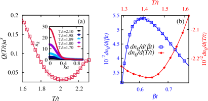
We plot vs in Fig. 10(a). exhibits a minimum at . In the inset, we show the evolution of the momentum distribution function as the temperature of the system is reduced. This result is compatible with the critical temperature found for the homogeneous system . In principle, similar ideas as the ones presented in Ref. Pollet et al., 2010 could be used to devise a quantity to locate the critical parameters in 2D. In that case, however, the structure of the momentum distribution is different because the transition is in another universality class. As a result, the LDA integrals for the central peak and the derivatives of the momentum distribution get substantially modified. We find that both the central peak and the derivatives of are critical in 2D because the LDA integrals of those quantities diverge in the center of the trap where the system is critical. Hence, one cannot define a , as done in 3D, that will exhibit a minimum at .
In Fig. 10(b), we also display results obtained for () in the same system. The temperature at which the maximum (minimum) occurs for those quantities exhibits a larger deviation from , from the homogeneous case, than . However, with increasing system size, we find that the maxima of (minima of ) slowly approach the homogeneous result. In experiments where the system sizes are much larger than the ones studies here, we expect that and will both produce accurate results for .
In Fig. 11, we present a summary of our estimates of the critical parameters based on the local compressibility, the derivatives of with respect to , and Eq. (35). The method based on is found to be more accurate than those based on and the local compressibility. This is understandable because the former approach uses precise information of the nature and universality class of the transition in 3D. Nevertheless, as argued before, we anticipate that if one decreases the strength of the confining potential and increases the number of bosons, as to reach the system sizes that are studied experimentally, then will provide accurate results (at least similar to the ones obtained in 2D). This effect is studied in Fig. 11 where we show the evolution of the critical temperature at the tip of the lobe as a function of system size. As the strength of the confining potential is decreased and the size of the system is increased, the estimate of the critical temperature based on tends to increase and approach in the homogeneous system. The method based on the local compressibility is found to be inadequate close to the tip of the lobe. This is because the maximum of becomes very broad and finite-size effects are stronger. In that regime, one also needs a higher accuracy in the determination of the density in order to accurately compute the local compressibility. In spite of this, in 3D, the method based on the local compressibility yields more accurate results than in 2D (compare Figs. 9 and 11).
V Conclusions
We have presented a detailed study of the finite temperature phase diagram of strongly correlated bosons in the hard-core limit (or the model) in two and three dimensions. The critical parameters in the homogeneous case were determined through a finite-size scaling analysis of the superfluid stiffness and the condensate fraction. We introduced an approach to estimate the critical temperature from measurements of in finite systems. It makes use of the behavior of the derivative and we derived finite-size scaling relations that can be used to extrapolate the results to the thermodynamic limit. This approach can be applied to systems that exhibit a diverging zero-momentum occupation in any dimension, irrespective of the universality class to which the transition belongs. We showed that this method is also accurate in 2D, where the system does not exhibit BEC. Furthermore, we computed the phase diagram using mean-field theory and found it to be quantitatively quite different from the results of numerically exact QMC simulations in 2D and 3D. Hence, for this model, thermal and quantum fluctuations are strong even in three dimensions, and mean-field theory is a poor approximation.
In the presence of an additional confining potential, we proved that the Bose-Hubbard model does not exhibit finite-temperature BEC in two dimensions, provided that density remains finite across the entire system in the thermodynamic limit. Moreover, we considered measurements of the critical temperature and chemical potential of the homogeneous system based on experimentally measurable quantities such as the momentum distribution function and the local density profile. The accuracy of each method discussed depends on the dimensionality of the system and the range of temperatures and chemical potentials considered. In two dimensions, we found that the approach introduced in this work, based on the derivatives of with respect to , is accurate in all regions of the phase diagram. A method based on the measurement of the local density was found to be reliable when is low, while close to the tip of the superfluid lobe this approach is less effective even when the trap is very shallow. This can be understood to be due to the strong deviations from the LDA close to the tip of the superfluid lobe. A quantitative account of these deviations based on trapped finite-size scaling, as presented in Ref. ceccarelli_vicari_12, and ceccarelli_torrero_12, , would in principle allow one to perform an accurate size-scaling analysis in the presence of the confining potential, which might potentially improve the capabilities of the methods based on the measurements of the density profile. The accuracy of the latter method improves in 3D, but still remains inadequate as one approaches the tip of the superfluid lobe. In three dimensions, the approach based on was found to be the most accurate.
Acknowledgements.
This work was supported by the U.S. Office of Naval Research under Award No. N000140910966. We thank Nikolai Prokof’ev, Itay Hen, and Rong Yu for useful discussions.Appendix A Differences between and
We briefly illustrate, by means of a simple analysis, why the estimate of the critical temperature based on differs from the estimate based on . We also discuss under which conditions the two estimates should approach each other.
We consider to be the zero momentum occupation in the vicinity of . Its first derivative, which exhibits a maximum at , can be written as
| (36) |
where the curvature of the parabola is , the height of the maximum is , and is assumed to be very close to . If instead we now compute , we anticipate a minimum of this function located at a temperature given by
| (37) |
In general, the position of the minimum as a function of depends on the position of the maximum , its curvature , and its height . However, in the limit of very large system sizes and very shallow traps, one expects the maximum of the derivative to be very sharp. In our simple example, this regime corresponds to a large value of the curvature, i.e., , which implies that .
References
- Daunt and Smith (1954) J. G. Daunt and R. S. Smith, Rev. Mod. Phys. 26, 172 (1954).
- Brutel et al. (1993) C. Bruder, R. Fazio and G. Schön , Phys. Rev. B 47, 342 (1993).
- giamarchi et al. (2008) T. Giamarchi, C. Rüeg, and O. Tchernyshyov , Nature Phys. 4, 198 2008.
- Bloch et al. (2008) I. Bloch, J. Dalibard, and W. Zwerger, Rev. Mod. Phys. 80, 885 (2008).
- (5) M. A. Cazalilla, R. Citro, T. Giamarchi, E. Orignac, and M. Rigol, Rev. Mod. Phys. 83, 1405 (2011).
- Fisher et al. (1989) M. P. A. Fisher, P. B. Weichman, G. Grinstein, and D. S. Fisher, Phys. Rev. B 40, 546 (1989).
- Jaksch et al. (1998) D. Jaksch, C. Bruder, J. I. Cirac, C. W. Gardiner, and P. Zoller, Phys. Rev. Lett. 81, 3108 (1998).
- Stöferle et al. (2004) T. Stöferle, H. Moritz, C. Schori, M. Köhl, and T. Esslinger, Phys. Rev. Lett. 92, 130403 (2004).
- Spielman et al. (2007) I. B. Spielman, W. D. Phillips, and J. V. Porto, Phys. Rev. Lett. 98, 080404 (2007).
- Jimenez-Garcia et al. (2010) K. Jiménez-García, R. L. Compton, Y. -J. Lin, W. D. Phillips, J. V. Porto, and I. B. Spielman, Phys. Rev. Lett. 105, 110401 (2010).
- Greiner et al. (2002) M. Greiner, O. Mandel, T. Esslinger, T. W. Hänsch, and I. Bloch, Nature (London) 415, 39 (2002a).
- Trotzky et al. (2010) S. Trotzky, L. Pollet, F. Gerbier, U. Schnorrberger, I. Bloch, N. V. Prokof’ev, B. Svistunov, and M. Troyer, Nature Phys. 6, 998 (2010).
- Schweikhard et al. (2007) V. Schweikhard, S. Tung, and E. A. Cornell, Phys. Rev. Lett. 99, 030401 (2007).
- Trombettoni, Smerzi, and Sodano (2005) A. Trombettoni, A. Smerzi, and P. Sodano, New J. Phys. 7, 57 (2005).
- (15) X. Zhang, C.-L. Hung, S.-K. Tung, and C. Chin, Science 335, 1070 (2012).
- Batrouni et al. (2002) G. G. Batrouni, V. Rousseau, R. T. Scalettar, M. Rigol, A. Muramatsu, P. J. H. Denteneer, and M. Troyer, Phys. Rev. Lett. 89, 117203 (2002).
- (17) M. Rigol, G. G. Batrouni, V. G. Rousseau, and R. T. Scalettar, Phys. Rev. A 79, 053605 (2009).
- (18) M. Rigol, A. Muramatsu, G. G. Batrouni, and R. T. Scalettar, Phys. Rev. Lett. 91, 130403 (2003).
- (19) S. Wessel, F. Alet, M. Troyer, and G. G. Batrouni, Phys. Rev. A 70, 053615 (2004).
- (20) M. Campostrini and E. Vicari, 2010b, Phys. Rev. A 81, 023606.
- (21) M. Campostrini and E. Vicari, 2010a, Phys. Rev. A 81, 063614.
- clade et al. (2009) P. Cladé, C. Ryu, A. Ramanathan, K. Helmerson, and W. D. Phillips, Phys. Rev. Lett. 102, 170401 (2009).
- Tung et al. (2010) S. Tung, G. Lamporesi, D. Lobser, L. Xia, and E. A. Cornell, Phys. Rev. Lett. 105, 230408 (2010).
- Xu et al. (2006) K. Xu, Y. Liu, D. E. Miller, J. K. Chin, W. Setiawan, and W. Ketterle, Phys. Rev. Lett. 96, 180405 (2006).
- Chin et al. (2006) J. K. Chin, D. E. Miller, Y. Liu, C. Stan, W. Setiawan, C. Sanner, K. Xu, and W. Ketterle, Nature (London) 443, 961 (2006).
- Kashurnikov et al. (2002) V. A. Kashurnikov, N. V. Prokof’ev, and B. V. Svistunov, Phys. Rev. A 66, 031601(R) (2002).
- Diener et al. (2007) R. B. Diener, Q. Zhou, H. Zhai, and T.-L. Ho, Phys. Rev. Lett. 98, 180404 (2007).
- Kato et al. (2008) Y. Kato, Q. Zhou, N. Kawashima, and N. Trivedi, Nature Phys. 4, 617 (2008).
- Pollet et al. (2010) L. Pollet, N. V. Prokof’ev, and B. V. Svistunov, Phys. Rev. Lett. 104, 245705 (2010).
- Fölling et al. (2006) S. Fölling, A. Widera, T. Müller, F. Gerbier, and I. Bloch, Phys. Rev. Lett. 97, 060403 (2006).
- Zhou et al. (2009) Q. Zhou, Y. Kato, N. Kawashima, and N. Trivedi, Phys. Rev. Lett. 103, 085701 (2009).
- Ho and Zhou (2010) T.-L. Ho, and Q. Zhou, Nature Phys. 6, 131 (2010).
- Nascimbene, Navon, Chevy, and Salomon (2010) S. Nascimbène, N. Navon, F. Chevy, and C. Salomon, New J. Phys. 12, 103026 (2010).
- (34) S. Fang, C.-M. Chung, P. N. Ma, P. Chen, and D.-W. Wang, Phys. Rev. A 83, 031605(R) (2011).
- Hazzard and Mueller (2011) K. R. A. Hazzard, and E. J. Mueller, Phys. Rev. A 84, 013604 (2011).
- Gemelke et al. (2009) N. Gemelke, X. Zhang, C.-L. Hung, and C. Chin, Nature (London) 460, 995 (2009).
- Sherson et al. (2010) J. F. Sherson, C. Weitenberg, M. Endres, M. Cheneau, I. Bloch, and S. Kuhr, Nature (London) 467, 68 (2010).
- Ma, Pollet and Troyer (2010) P. N. Ma, L. Pollet, and M. Troyer, Phys. Rev. A 82, 033627 (2010).
- Bakr et al. (2010) W. S. Bakr, A. Peng, M. E. Tai, R. Ma, J. Simon, J. I. Gillen, S. Folling, L. Pollet, and M. Greiner, Science 329, 547 (2010).
- Zhang, Hung, Tung, Gemelke, Chin (2011) X. Zhang, C.-L. Hung, S.-K. Tung, N. Gemelke, and C. Chin, New J. Phys. 13, 045011 (2011).
- (41) E. Duchon, Y. Kato , N. Trivedi, arXiv:1112.0592v1. M. Tiersch and H. J. Briegel, arXiv:1204.4179v1.
- Kruger et al. (2007) P. Krüger, Z. Hadzibabic, and J. Dalibard, Phys. Rev. Lett. 99, 040402 (2007).
- Nascimbene et al. (2010) S. Nascimbène, N. Navon, K. J. Jiang, F. Chevy, and C. Salomon, Nature (London) 463, 1057 (2010).
- Hung et al. (2011) C.-L. Hung, X. Zhang, N. Gemelke, and C. Chin, Nature (London) 470, 236 (2011).
- Mermin and Wagner (1966) N. D. Mermin, and H. Wagner, Phys. Rev. Lett. 17, 1133 (1966).
- Hohenberg (1967) P. C. Hohenberg, Phys. Rev. 158, 383 (1967).
- (47) V. L. Berezinskii, Sov. Phys. JETP 34, 610 (1972).
- (48) J.M. Kosterlitz and D.J. Thouless, J. Phys. C 6, 1181 (1973).
- Li and Teitel (1989) Y.-H. Li and S. Teitel, Phys. Rev. B 40, 9122 (1989).
- Salamon, Shi, Overend, and Howson (1993) M. B. Salamon, J. Shi, N. Overend, and M. A. Howson, Phys. Rev. B 47, 5520 (1993).
- Overend, Howson, and Lawrie (1994) N. Overend, M. A. Howson, and I. D. Lawrie, Phys. Rev. Lett. 72, 3238 (1994).
- (52) M. Campostrini, M. Hasenbusch, A. Pelissetto, and E. Vicari, Phys. Rev. B 74, 144506 (2006).
- (53) E. Burovski, J. Machta, N. Prokof’ev, and B. Svistunov, Phys. Rev. B 74, 132502 (2006).
- Campostrini et al. (2001) M. Campostrini, M. Hasenbusch, A. Pelissetto, P. Rossi, and E. Vicari, Phys. Rev. B 63, 214503 (2001).
- (55) M. Hasenbusch and T. Török, J. Phys. A: Math. Gen. 32, 6361 (1999).
- (56) T. Matsubara and H. Matsuda, Prog. Theor. Phys. 16, 569 (1956).
- Sandvik and Kurkijarvi (1991) A. W. Sandvik, and J. Kurkijärvi, Phys. Rev. B 43, 5950 (1991).
- (58) A. W. Sandvik, J. Phys. A 25 3667 (1992).
- Dorneich and Troyer (2001) A. Dorneich and M. Troyer, Phys. Rev. E 64, 066701 (2001).
- (60) E. Loh, D. J. Scalapino, and P. M. Grant, Phys. Rev. B 31, 4712 (1985).
- (61) H.-Q. Ding, M. S. Makivić, Phys. Rev. B 42, 6827 (1990).
- (62) H.-Q. Ding, Phys. Rev. B 45, 230 (1992).
- (63) K. Harada and N. Kawashima, Phys. Rev. B 55, R11949 (1997).
- (64) E. L. Pollock and D. M. Ceperley, Phys. Rev. B 36, 8343 (1987).
- (65) P. Olsson, Phys. Rev. B 52, 4526 (1995).
- (66) H. Weber and P. Minnhagen, Phys. Rev. B 37, 5986 (1988).
- (67) Note that, in Ref. harada_kawashima_97, , a more sophisticated fitting approach allowed them to obtain the critical value with a higher accuracy that the one we achieve in here.
- (68) M. Hasenbusch, J. Phys. A: Math. Gen. 38, 5869 (2005).
- (69) D. J. Amit, Y. Y. Goldschmidt and S. Grinstein, J. Phys. A: Math. Gen. 13 585 (1980).
- (70) R. Kenna, A. C. Irving, Phys. Lett. B 351 273 (1995).
- (71) M. H. Pedersen and T. Schneider, Phys. Rev. B 53, 5826 (1996).
- (72) N. Kawashima, J. Phys. Soc. Jpn. 73, 3219 (2004).
- (73) R. G. Melko and D. J. Scalapino, Phys. Rev. B 71, 094511 (2005).
- (74) M. E. Fisher, M. N. Barber, and D. Jasnow, Phys. Rev. A 8, 1111 (1973).
- (75) N. Laflorencie, Europhys. Lett. 99, 66001 (2012).
- (76) O. Penrose and L. Onsager, Phys. Rev. 104, 576 (1956).
- (77) A. Pelissetto and E. Vicari, Phys. Rep. 368, 549 (2002).
- Sheshadri (1993) K. Sheshadri, H. R. Krishnamurthy, R. Pandit, and T.V. Ramakrishnan, Europhys. Lett. 22, 257 (1993).
- Dalfovo et al. (1999) F. Dalfovo, S. Giorgini, L. P. Pitaevskii, and S. Stringari, Rev. Mod. Phys. 71, 463 (1999).
- (80) W. J. Mullin, J. Low Temp. Phys. 106, 615 (1997).
- horn (2000) R. A. Horn and C. R. Johnson Matrix Analysis, (Cambridge University Press, New York), (1985).
- (82) C. E. Campbell, K. E. Kürten, M. L. Ristig, and G. Senger, Phys. Rev. B 30, 3728 (1984).
- (83) F. Alet, S. Wessel, and M. Troyer, Phys. Rev. E 71, 036706 (2005).
- Zhou et al. (2010) Q. Zhou, Y. Kato, N. Kawashima, and N. Trivedi, Phys. Rev. Lett. 105, 199602 (2010).
- (85) G. Ceccarelli, C. Torrero, and E. Vicari, Phys. Rev. A 85, 023616 (2012).
- (86) G. Ceccarelli and C. Torrero, Phys. Rev. A 85, 053637 (2012).