The mass distribution of the Fornax dSph:
constraints from its globular cluster distribution

Abstract

Uniquely among the dwarf spheroidal (dSph) satellite galaxies of the Milky Way, Fornax hosts globular clusters. It remains a puzzle as to why dynamical friction has not yet dragged any of Fornax’s five globular clusters to the centre, and also why there is no evidence that any similar star cluster has been in the past (for Fornax or any other dSph). We set up a suite of 2800 $N$-body simulations that sample the full range of globular-cluster orbits and mass models consistent with all existing observational constraints for Fornax. In agreement with previous work, we find that if Fornax has a large dark-matter core then its globular clusters remain close to their currently observed locations for long times. Furthermore, we find previously unreported behaviour for clusters that start inside the core region. These are pushed out of the core and gain orbital energy, a process we call ‘dynamical buoyancy’. Thus a cored mass distribution in Fornax will naturally lead to a shell-like globular cluster distribution near the core radius, independent of the initial conditions. By contrast, CDM-type cusped mass distributions lead to the rapid infall of at least one cluster within $\Delta t=1$-2 Gyr, except when picking unlikely initial conditions for the cluster orbits ($\sim 2\%$ probability), and almost all clusters within $\Delta t=10$ Gyr. Alternatively, if Fornax has only a weakly cusped mass distribution, dynamical friction is much reduced. While over $\Delta t=10$ Gyr this still leads to the infall of 1-4 clusters from their present orbits, the infall of any cluster within $\Delta t=1$-2 Gyr is much less likely (with probability 0-70%, depending on $\Delta t$ and the strength of the cusp). Such a solution to the timing problem requires (in addition to a shallow dark-matter cusp) that in the past the globular clusters were somewhat further from Fornax than today; they most likely did not form within Fornax, but were accreted.

1 Introduction

The Fornax dwarf spheroidal (dSph) galaxy is the most massive undisrupted dSph satellite of the Milky Way (Walker et al., 2009). Like all dSphs it is dark matter dominated even in its central regions. It is unique among the undisrupted dSphs in having globular clusters; it has five, with three of them at a projected distance outside of the half light radius (see table 1). There is also evidence of two shell-like structures, which may be the remnants of a merger occurring more than 2 Gyr ago (Coleman et al., 2004; Coleman et al., 2005).

One apparent paradox about these clusters is that, because they appear to orbit in a massive background of dark matter, they should be affected by dynamical friction which will cause their orbits to decay. Fornax’s globular clusters are metal poor and very old, comparable to the oldest globular clusters in the Milky Way with ages of the order of a Hubble time (Buonanno et al., 1998, 1999; Mackey & Gilmore, 2003a; Greco et al., 2007). During their lifetime it would be expected that they fall to the centre of Fornax and form a nuclear star cluster (Tremaine, Ostriker & Spitzer Jr., 1975; Tremaine, 1976). However, no bright stellar nucleus is observed in Fornax, or in fact any other dSph. This is known as the timing problem for Fornax’s clusters because it seems highly improbable that Fornax’s globular clusters would be observed just briefly before they fall into the core.

Several solutions to the timing problem have been proposed. Oh, Lin & Richer (2000) suggested two ideas. First, that a population of black holes transferred energy to the clusters through close encounters; and second, that a strong tidal interaction between the Milky Way and Fornax could inject energy into their orbits. There is no observational evidence for a population of black holes in the centre of Fornax, while the currently observed proper motion indicates that the orbit of Fornax around the Milky Way never takes it closer than at present (Dinescu et al. 2004; Lux, Read & Lake 2010). Thus, both ideas appear to be disfavoured. Angus & Diaferio (2009) proposed that all but the most massive cluster could avoid sinking into the centre of Fornax if their current distance is much larger than projected but still within the tidal radius of Fornax of $\sim 1.9\,$kpc. However, this (i) requires special arrangement of the current projected positions and (ii) stills leaves a timing problem for the most massive cluster and is therefore not a complete solution (moreover, their analysis was based on Chandrasekhar’s simple dynamical-friction formula, which is not suitable for accurate estimates).

Using numerical simulations and analytic arguments Goerdt et al. (2006) proposed that the current distribution of the Fornax clusters can be explained by the diminution of dynamical friction on the edge of a cored matter distribution which causes the clusters to remain outside the dark matter core radius. Dynamical reasons for this ‘core-stalling’ effect have been explored in Read et al. (2006), Inoue (2009), and Cole, Dehnen & Wilkinson (2011). Support for this result was provided by Sánchez-Salcedo, Reyes-Iturbide & Hernandez (2006) who showed that a cored matter distribution in dwarf galaxies can significantly delay the infall times of the globular clusters (even if Chandrasekhar’s simple dynamical-friction formula is used).

Measuring and/or constraining the dark-matter distribution in Fornax is interesting as a test of our current cosmological model. Collisionless cosmological simulations (which ignore the effects of baryons) predict a universal density distribution for dark matter halos, with a central density cusp $\rho\propto r^{-\gamma}$ where $\gamma\sim 1$ (Dubinski & Carlberg, 1991; Navarro, Frenk & White, 1996). If the dark matter distribution in Fornax is found to deviate strongly from this prediction, this could imply that baryons have an important dynamical role in shaping the central dark matter distribution in dwarf galaxies (e.g. Navarro, Eke & Frenk 1996, El-Zant, Shlosman & Hoffman 2001, Read & Gilmore 2005, Goerdt et al. 2010, Cole et al. 2011, Pontzen & Governato 2012), or that we must turn to more exotic cosmological models (e.g. Tremaine & Gunn 1979, Kochanek & White 2000, Hogan & Dalcanton 2000, Strigari et al. 2006, Villaescusa-Navarro & Dalal 2011, Maccio’ et al. 2012).

The first evidence that dSphs may have a constant density core came from Kleyna, Wilkinson, Gilmore & Evans (2003) who found indirect evidence for a core in the Ursa Minor dSph. The Milky Way dSphs have been observed intensively in recent years, primarily because these systems are the most dark-matter dominated known. They contain mostly intermediate or old stellar populations which are likely to be well mixed in the dark matter potential because star formation ceased many dynamical times ago. This in turn implies that they are ideal laboratories for studying the mass structure of their dark matter halos. The intense observational effort means that there is a wealth of kinematical data available to form the basis for theoretical models of these systems. One line of approach has been based on the Jeans equations where a parametric light profile for the stars is assumed and a velocity dispersion profile is derived based on a underlying parameterised dark matter profile (Peñarrubia, McConnachie & Navarro 2008, Strigari et al. 2008, Walker et al. 2009). This approach has its drawbacks (see for example Amorisco & Evans 2011b). Most importantly, the degeneracy between the mass profile and the velocity anisotropy (which is poorly constrained), means that both cusped and cored density distributions are consistent with even the latest data. However, modelling the dSphs as two chemically distinct populations with different scale lengths, it appears that this degeneracy can be broken (Battaglia et al., 2008; Amorisco & Evans, 2011a, b; Walker & Peñarrubia, 2011); the results favour a cored density distribution in the two dSph galaxies best analysed to date: Fornax and Sculptor (but see Breddels et al., 2012).

In this paper, we we follow the work of Goerdt et al. (2006) by examining what the current location of the globular clusters can tell us about Fornax’s mass distribution. Our work improves on this previous analysis in several key respects: (i) we use several mass models for the underlying potential in Fornax that sample the full range consistent with the latest data; (ii) we use the latest data for Fornax’s globular clusters as constraints on their phase space distribution; and (iii) we run thousands of $N$-body models to sample the uncertainties in the cluster distribution and Fornax mass model.

This large search of the available parameter space allows us to address whether or not there are multiple solutions to Fornax’s timing problem. To focus the discussion, we phrase the timing problem as a contradiction with either of the following two hypotheses

1. The Fornax globular cluster system is in a near-steady state, consequently none of the globular clusters should fall into the core of Fornax within a Hubble time.

2. Our present cosmic epoch of observing Fornax is not special, consequently the system does not evolve significantly on a time scale short compared to a Hubble time. In particular, within 1-2 Gyr none of the clusters should fall into the core of Fornax with high probability.

The first hypothesis can be justified by the assumption that the present state of Fornax’s globular cluster system is representative also for its past. This assumption, however, is not necessary, as one can easily think of alternative scenarios. The second hypothesis, on the other hand, is harder to avoid and similar to the cosmological principle, though here expressed in terms of the epoch of observation rather than its vantage point and orientation. We will refer to contradictions with these hypotheses as the long-term and immediate timing problem, respectively.

This paper is organised as follows. Section 2 reviews the properties of the Fornax system relevant for our study, Section 3 details our modelling approach, Sections 4&5 present the simulations results and assess the probability that none of the five clusters will sink into the core of Fornax within either 1–2 Gyr or a Hubble time. Finally, in Section 6 we discuss the implications of our results and draw our conclusions.

Object	log$M$ a		$M$ a	$r_{\mathrm{c}}$ a	$R_{\mathrm{p}}$ a	$d_{\mathrm{los}}$		$\Delta\upsilon_{\mathrm{los}}$d
	$[\mbox{M${}_{\odot}$}]$		[$10^{5}\mbox{M${}_{\odot}$}$]	[pc]	[kpc]	[kpc]		[km s-1]
dSph	$8.15^{\,+\,0.19}_{\,-\,0.37}{}^{e}$		1420 e	668e	-	137.0$\;\!\pm\;\!$	13.b,f	-
						138.0$\;\!\pm\;\!$	8.0g
GC1	4.57$\;\!\pm\;\!$	0.13	0.37	10.03	1.61	130.6$\;\!\pm\;\!$	3.0b	-
GC2	5.26$\;\!\pm\;\!$	0.12	1.82	15.81	1.05	136.1$\;\!\pm\;\!$	3.1b	–1.2$\;\!\pm\;\!$	4.6
GC3	5.56$\;\!\pm\;\!$	0.12	3.63	11.60	0.43	135.5$\;\!\pm\;\!$	3.1b	7.1$\;\!\pm\;\!$	3.9
GC4	5.12$\;\!\pm\;\!$	0.24	1.32	11.75	0.24	134.0$\;\!\pm\;\!$	6.0c	5.9$\;\!\pm\;\!$	3.4
GC5	5.25$\;\!\pm\;\!$	0.20	1.78	11.38	1.43	140.6$\;\!\pm\;\!$	3.2b	8.7$\;\!\pm\;\!$	3.6

Table 1: Data for the Fornax system. Column 3 shows the most likely mass from column 2. $r_{\mathrm{c}}$ is the King (1962)model core radius for the globular clusters, and the half-light radius for the dSph. $R_{\mathrm{p}}$ is the projected distance of the cluster from the centre of Fornax. $d_{\mathrm{los}}$ is the distance to each cluster and $\Delta\upsilon_{\mathrm{los}}$ the line-of-sight velocity relative to Fornax itself. References: ^aMackey & Gilmore (2003b),^bMackey & Gilmore (2003a),^cGreco et al. (2007),^dMateo et al. (1991),^eWalker et al. (2009),^fBuonanno et al. (1999),^gMateo (1998),^hBuonanno et al. (1998).

2 The Fornax system

We summarise in Table 1 the most relevant data for our study and their origin.

2.1 The dSph

As already discussed above, Fornax is the most massive of the Milky Way’s dSph (except possibly for disrupted objects such as Sgr dwarf) and unique amongst (undisrupted) dSph to host a globular cluster system. The very fact that Fornax can hold onto a globular-cluster system implies that Galactic tides cannot be strong enough to pull these clusters off. This in turn requires that its Galactic orbit never carries Fornax too close to the Milky Way, where the tidal forces become exceedingly strong.

Lux, Read & Lake (2010) estimate the peri-galactic radius of Fornax, based on its observed position, distance, radial velocity and proper motion, to be 100–130 kpc, which indeed is only slightly smaller than its current distance of about 140 kpc (see Table 1).

Based on this result, we estimate the tidal radius for Fornax using the method of Read et al. (2006), where the dSph is modelled as a spherical satellite orbiting the Milky Way represented by a Hernquist (1990) model. We then solve equation (7) of Read et al. (2006), which accounts for the orbit of the satellite about the host, and the orbits of the stars within the satellite. We find a tidal radius of 1.8–2.8 kpc, based on a the range of masses for Fornax given in Table 2 and using the extremal values for the the orbital data taken from Lux et al. (2010) and a total (extended) mass for the Milky Way of $1{-}2\times 10^{12}\,\mbox{M${}_{\odot}$}$.

2.2 The globular clusters

Our principle sources for globular-cluster data are those published by Mackey & Gilmore (2003a, b) and Greco et al. (2007) who have carried out thorough surveys of the Fornax globular clusters. For our purposes the main data required are the clusters’ masses, sizes, three dimensional positions and velocities.

The best estimates for these quantities are given in Table 1. The values for the core radius $r_{\mathrm{c}}$ of each cluster are based on the surface brightness profiles calculated in Mackey & Gilmore (2003b). These are Elson, Fall & Freeman (1987, EEF) models and the King (1962) model core radius $r_{\mathrm{c}}$ is related to the EFF scale parameter $a$ by $r_{\mathrm{c}}=a(2^{2/\gamma}-1)^{1/2}$, where $\gamma$ is the power law slope of the surface brightness at large radii.

Figure 1: Distribution of the Fornax globular clusters in mass and projected distance from the centre of the Fornax dSph. The dashed vertical line indicates the stellar half-light radius of the dSph.

Fig. 1 plots the distribution of the five Fornax globular clusters in mass $M$ and projected radius $R_{\mathrm{p}}$ from the dSph. There are two interesting observations to be made from this figure. First, the radial distribution of clusters is consistent with that of the stars within Fornax: there is about half of the total cluster light within the stellar half-light radius of 668 pc. There are two possible interpretations of this. Either it is a coincidence, or the formation histories of the clusters and the Fornax galaxy are closely related, in particular, the clusters formed within the same entities as the stars.

Second, there is a weak correlation between $M$ and $R_{\mathrm{p}}$. In particular, the lightest cluster is furthest away from Fornax and the heaviest is the second closest. The remaining three are about equally massive and cover a spread of $R_{\mathrm{p}}$. This correlation is in the sense expected from mass segregation such as driven by dynamical friction.

3 Modelling Approach

The basis for our approach is to take the most up-to-date observations of Fornax’s globular clusters and combine these with plausible mass models consistent with the latest kinematic data for Fornax’s stars. We then create, for each Fornax mass model, initial conditions for the Fornax globular-cluster system, which are consistent with the relevant observations, and evolve them for ten Gyr into the future.

Model	Name	$\gamma_{0}$	$\gamma_{\infty}$	$\eta$	$M_{\infty}$	$r_{\mathrm{s}}$	$\gamma_{100\mathrm{pc}}$	$M(1.8\mathrm{kpc})$
LC	large core	0.07	4.65	3.7	$8.00\times 10^{8}$	1.4	0.1	$4.12\times 10^{8}$
WC	weak cusp	0.08	4.65	2.77	$1.23\times 10^{8}$	0.62	0.1	$1.03\times 10^{8}$
IC	intermediate cusp	0.13	4.24	1.37	$1.51\times 10^{8}$	0.55	0.5	$1.03\times 10^{8}$
SC	steep cusp	0.52	4.27	0.93	$1.98\times 10^{8}$	0.80	1.0	$1.07\times 10^{8}$

Table 2: Parameters for halo mass models (equation 1) used in the simulations ($\gamma_{0}$, $\gamma_{\infty}$, $\eta$, $M_{\infty}$, $r_{\mathrm{s}}$), as well as the resulting logarithmic density slope $\gamma(r)\equiv-\mathrm{d}\ln\rho/\mathrm{d}\ln r$ at 100 pc and the mass within 1.8kpc, our lower limit for the tidal radius of Fornax. Radii are given in kpc and masses in M_⊙.

3.1 Mass models for Fornax

Wilkinson et al. (2002) and Kleyna et al. (2002) demonstrated that the mass-anisotropy degeneracy inherent in kinematic modelling can be broken using distribution-function modelling of sufficiently large kinematic data sets. To take full advantage of the recent data set of more than two thousand individual stellar velocities in Fornax (Walker et al., 2009), Wilkinson et al. (in preparation) apply the Markov-Chain-Monte-Carlo (MCMC) technique to dynamical and mass models of Fornax. The mass profile and stellar-luminosity profile are modelled independently using spherical double-power-law profiles of the form

$$\rho_{\mathrm{model}}(r)=\rho_{0}\,\left(\frac{r}{r_{\mathrm{s}}}\right)^{-\gamma_{0}}\left(1+\left(\frac{r}{r_{\mathrm{s}}}\right)^{\eta}\right)^{\frac{\gamma_{0}-\gamma_{\infty}}{\eta}}.$$ (1)

The stellar distribution functions are calculated numerically following the approach of Gerhard (1991) and Saha (1992) allowing various velocity anisotropy profiles. As in the earlier work (Wilkinson et al., 2002; Kleyna et al., 2002), the models are compared to the data on a star-by-star basis.

Further details of the modelling and its results will be presented elsewhere. Here, we simply use the above MCMC model ensemble to inform our choice of halo models. Rather than considering a single best-fit model of Fornax, we select four mass models, each of the form (1) but truncated at very large radii via

$$\rho(r)=\rho_{\mathrm{model}}(r)\;\mathrm{sech}(r/10\mathrm{kpc}),$$ (2)

and with parameter values as detailed in Table 2. These models span the range of models consistent with the kinematic data. The three models WC (weak cusp), IC (intermediate cusp) and SC (steep cusp) have parameters $\gamma_{0}$, $\gamma_{\infty}$, $\eta$, $r_{\mathrm{s}}$, and $M_{\infty}$ directly taken from the MCMC chain outputs, and refer to the highest likelihood models with density slope

$$\gamma(r)\equiv-\frac{\mathrm{d}\ln\rho}{\mathrm{d}\ln r}$$ (3)

of, respectively, 0.1, 0.5, and 1.0 at $r=100\,$pc.

The fourth model, LC (large core), was motivated by the recent work of Walker & Peñarrubia (2011). These authors applied a non-parametric statistical modelling technique to two chemically distinct stellar populations within Fornax to define the enclosed mass at the half light radii of the two populations. The resulting model possesses a large core with near-constant density and $\gamma\approx 0.1$ for $r\lesssim 500\,$pc.

The radial profiles of density, enclosed mass, and logarithmic density slope of the four mass models are shown in Fig. 2 for comparison. These models cover a wide range of inner density slopes, including shallow profiles, such as suggested by (Gilmore et al., 2007) based on observations of dSph galaxies, but also a steep cusp, such as predicted by cosmological simulations (Dubinski & Carlberg, 1991; Navarro et al., 1996). Note, however, that our models represent the overall mass distribution of Fornax including both the stars and the dark matter.

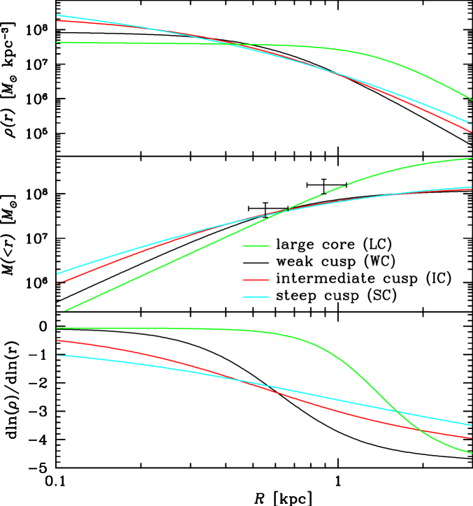
Figure 2: Radial profiles of density (top), enclosed mass (middle), and logarithmic density slope (bottom) for the four mass models used in our simulations (see also Table 2).The data points the middle panel correspond to the mass estimates by Walker & Peñarrubia (2011)for two chemically distinct sub-populations.

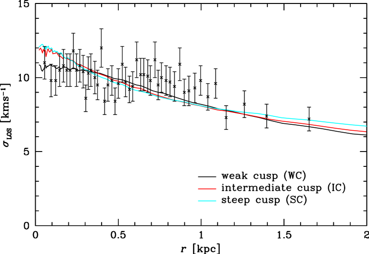
Figure 3: The observed stellar velocity dispersion for Fornax as a function of projected radius (Walker et al. 2007),and the simple predictions obtained for the four mass models used in this study under the assumption of isotropic velocities. The purpose of this comparison is not to assess the relative merit of the mass models, but merely to demonstrate that their normalisations are reasonable.

Figure 3 shows the stellar velocity dispersion for of our three MCMC-based Fornax models (curves) plotted together with the observed velocity dispersion as measured by Walker et al. (2007). The model velocity dispersions were calculated assuming an ergodic distribution function with a Plummer (1911) density profile with core radius 668 pc for the stellar component, but the respective halo model for the underlying mass distribution. In view of the fact that these simple ergodic models have not been fitted to the velocity-dispersion data (apart from the assumed mass models), they provide surprisingly good a description of these data. (This and the similarity between the model predictions is exactly the reason why inferring the mass profile from data like these is hardly possible.)

The large core model (LC) has been normalised to roughly agree with the estimates for the enclosed mass derived from two different tracer populations by Walker & Peñarrubia (2011) and plotted in Fig. 2.

3.2 Modelling the globular cluster system

If we compare the distance to the Fornax dSph with the distances to the individual clusters in Table 1, it can be seen that the measurements of the distances are not accurate enough to provide reliable three-dimensional locations within the dSph. We therefore draw for each simulation random line-of-sight distance offsets to Fornax from a uniform distribution between 0 and 2 kpc, the approximate tidal radius of the system (Walker & Peñarrubia, 2011). For the velocities, we choose a similar statistical approach by sampling the full space velocity from a bi-variate Gaussian distribution, specified by the total velocity dispersion $\sigma$ and the anisotropy parameter

$$\beta\equiv 1-\frac{\sigma_{\theta}^{2}+\sigma_{\phi}^{2}}{2\sigma_{r}^{2}}.$$ (4)

This is done in such a way that for clusters GC2-5 the line-of-sight velocity matches the observed value (which may be considered a prior for our sampling).

As the spatial distribution of the clusters is consistent with that of the stars in Fornax, it seems reasonable to base our kinematical parameters for the clusters on the observed stellar kinematics. The measured stellar velocity dispersion is approximately flat over the range of radii observed (Walker et al., 2007; Łokas, 2009), and we use $\sigma=10.5\,$km s^-1. For the velocity anisotropy we assume $\beta=-0.33$ as suggested for the stars (Łokas, 2009), i.e. a mild tangential bias, which gives $\sigma_{r}\approx 9.5\,$km s^-1 and $\sigma_{t}\approx 11\,$km s^-1.

With this modelling approach, in particular the wide range of initial radii sampled, we generate many different orbits for the globular clusters, covering the complete range of all possible orbits for them. By allowing such a wide distribution of cluster orbits, we can explore the effects of possible narrow choices for the cluster distribution function, such as preferably circular orbits, afterwards by restricting our analysis correspondingly.

3.3 $N$-body simulations

For each Fornax mass model, we ran 700 $N$-body simulations, each with different initial conditions for the five clusters.

The individual cluster positions and velocities are drawn as described in the previous sub-section and their masses are taken from Table 1. The clusters are represented by individual massive but softened particles with density profiles

$$\rho(r)\propto(r^{2}+\epsilon^{2})^{-7/2},$$ (5)

where $\epsilon=5\,$pc, comparable to the cluster core radii.

To generate the $N$-body initial conditions for the Fornax mass models, we sample positions from the density (2) and velocities from self-consistent ergodic distribution functions $f(E)$, which only depend on the specific orbital energy $E$, thus giving everywhere isotropic velocity distributions. The forces between particles representing Fornax are softened with softening length $\epsilon=10\,$pc.

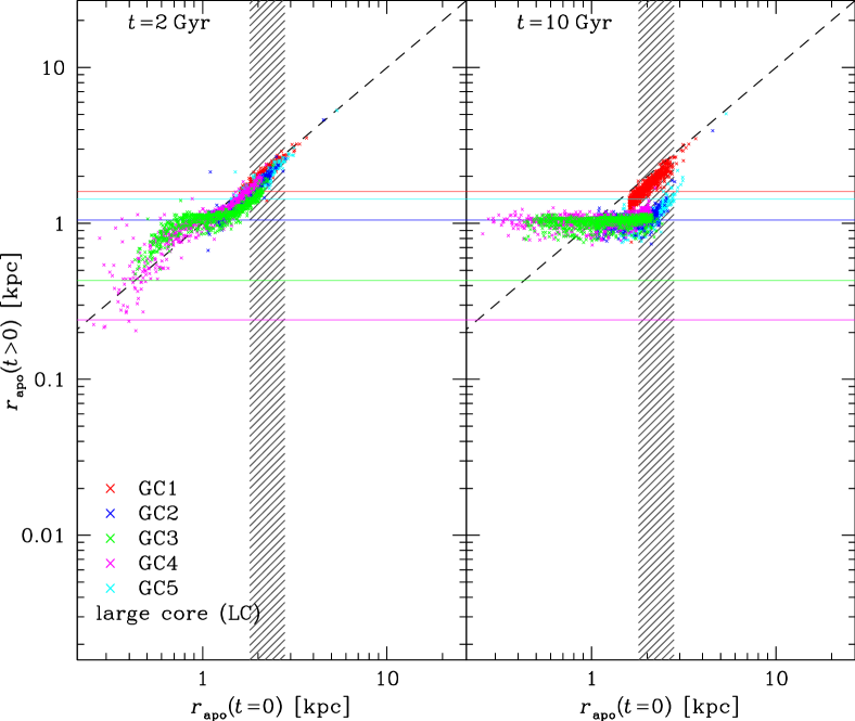
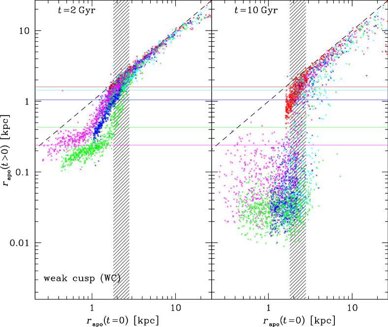
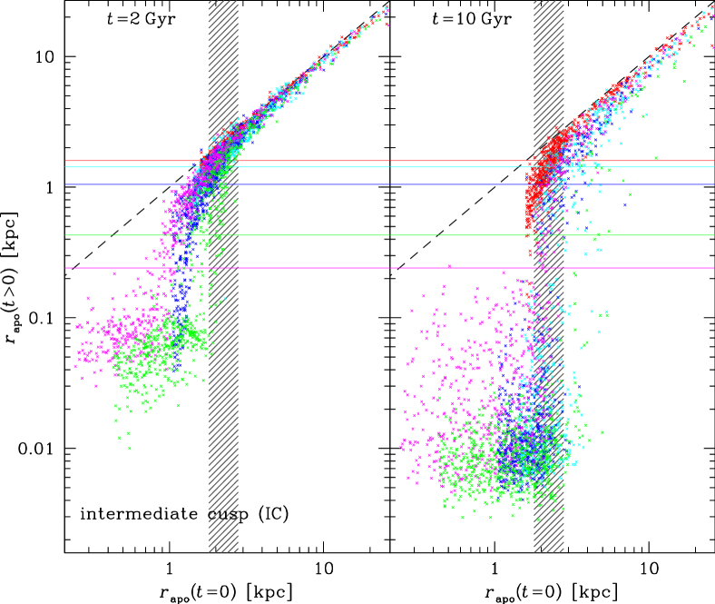
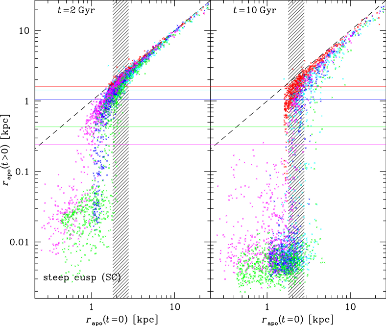
Figure 4: Apo-centric radii $r_{\mathrm{apo}}$ of the instantaneous cluster orbits after $t=2$ and 10 Gyr for all simulations per halo model (as indicated) plotted versus $r_{\mathrm{apo}}$ of the initial orbit. The shaded region indicates the most likely value for the current tidal radius of Fornax. Any initial $r_{\mathrm{apo}}$ greater than that would have been strongly affected (likely removed from Fornax) by the Galactic tidal field (not modelled in our simulations). The thin horizontal lines indicate the observed projected radius $R_{\mathrm{obs}}$ for each cluster, which is necessarily less than its initial $r_{\mathrm{apo}}$. Any final $r_{\mathrm{apo}}$ below these lines would be inconsistent with the present cluster location.

We enhance the resolution of the $N$-body model in the inner parts (where dynamical friction occurs) by increasing the sampling probability by a factor $g(E)^{-1}$ which is compensated by setting particle masses $\mu_{i}$ proportional to $g(E_{i})$. We used

$$g(E)\propto\frac{1+q\,r_{\mathrm{circ}}^{\eta}(E)}{r_{\mathrm{circ}}^{\eta}(E)+r_{s}^{\eta}}$$ (6)

with $q=4$ the ratio between maximum and minimum particle mass and $r_{\mathrm{circ}}(E)$ the radius of the circular orbit with specific energy $E$. Testing this method for our particular purposes, we found that it allows a reduction of $N$ to half at the same central resolution without any adverse effects. Based on convergence tests of decaying cluster orbits (see Appendix A), we use $N=2\times 10^{6}$ particles to sample each of the Fornax mass models.

The mass ratio of the lightest background particle in all our models to the lightest cluster is 1:1680 (in model WC) and that of the heaviest particle to the lightest cluster 1:62 (in model LC). The clusters orbit mainly within the high-resolution region of our models defined by the volume where the resolution is better than would have been achieved with the same number of particles of constant mass (within approximately 2 kpc).

The simulations are performed using the publicly available $N$-body code gyrfalcON, which uses Dehnen’s (2000, 2002) $\mathcal{O}(N)$ algorithm for force approximation. The total energy conservation was typically a few parts in $10^{4}$.

4 Raw simulation results

As detailed at the end of §3.2, our simulations cover a wide range of initial cluster orbits, some of which may not be very realistic. In this section we ignore any implications of our sampling of the initial cluster orbits and simply consider the individual simulations on their own merit.

For each simulation, we need to quantify in how much each simulated cluster has suffered from dynamical friction and has sunken into the core of the dSph. In this respect it is clearly better to use an orbital property instead of an instantaneous quantity, such as radius (projected or intrinsic). Therefore, we use as our main characteristic the apo-centric radius $r_{\mathrm{apo}}$ of the instantaneous cluster orbit. This is obtained from the cluster’s instantaneous angular momentum $L$ and specific energy $E$ as the larger of the two radii for which

$$E=\frac{L^{2}}{2r}+\Phi(r)$$ (7)

(the smaller is the peri-centric radius). $\Phi(r)$ is the instantaneous gravitational potential of the $N$-body model, estimated using spherical averaging. For a small fraction of simulated clusters, the initial orbits were unbound. Such simulations are discarded only for analysis of the affected cluster orbit, but not for the others.

For each of the four mass models of Table 2, Fig. 4 plots the distributions of each cluster orbit in initial and final $r_{\mathrm{apo}}$ at $t=2\,$Gyr and $t=10\,$Gyr in the left and right sub-panels, respectively.

4.1 Orbital decay after 2 Gyr

After 2 Gyr (left sub-panels in Fig. 4) $r_{\mathrm{apo}}$ is significantly less than initially for most orbits with initial $r_{\mathrm{apo}}<2-3\,$kpc, except for model LC, which we discuss separately in §4.3.

However, both GC1 (red) and GC5 (cyan) rarely sink substantially, and GC1 only ever falls into the centre of Fornax for the most cusped model SC. This is not surprising since GC1 is not only by far the lightest of the five clusters (see Table 1), but also the one furthest away (in projection) from the centre of Fornax and hence less likely to pass through high density regions. As such it requires most dynamical friction to fall into Fornax, but will suffer least, since drag force $\propto\mathrm{mass}^{2}\rho$. Though GC5 is five times more massive, it has the second greatest projected distance from the centre of Fornax and hence also suffers significantly less friction than the other clusters for most orbits sampled.

The remaining three clusters GC2-4 are all dragged inwards when initially $r_{\mathrm{apo}}<2-3\,$kpc, presenting the Fornax timing problem. For all of these clusters, orbits with initial $r_{\mathrm{apo}}\lesssim 1\,$kpc show similar effects of dynamical friction, presumably because orbits with apo-centres as small as that spend sufficient time in high-density regions to suffer substantially from dynamical friction.

Since $R_{\mathrm{p}}\leq r_{\mathrm{apo}}$, an initial $r_{\mathrm{apo}}\sim 1\,$kpc is the absolute possible minimum for GC2, which is observed at $R_{\mathrm{p}}=1.05\,$kpc. Consequently GC2 only rarely falls in as much as GC3 and GC4.

Apart from the initial $r_{\mathrm{apo}}$, the infall of these clusters depends most strongly on the inner density profile of the background mass distribution. Model SC shows the greatest effect of dynamical friction on the clusters. For GC3 and GC4, a significant proportion of the simulations find their instantaneous apo-centres inside 30 pc. GC2 does not show such a marked effect but a number of simulations already have an apo-centre inside 100 pc.

By contrast, model WC shows significantly reduced dynamical friction. GC3 again is most affected. However, even in the most extreme cases, the apo-centres have decayed to no less than $\sim 100\,$pc from the centre. In this model the logarithmic density slope $\gamma$ (equation 3) was initially only 0.1 at 100 pc, which implies a near-flat density profile within this radius. As expected, model IC is intermediate between models WC and SC.

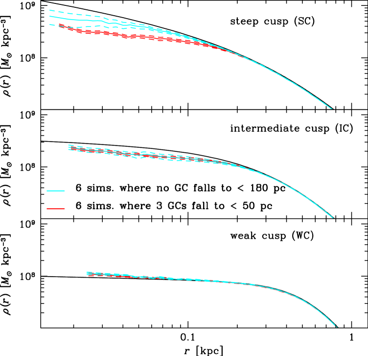
Figure 5: Ths initial (black) and final ($t=10\,$Gyr, coloured) density profile of six halo models (stacked $N$-body models) from simulations where either three clusters sunk into Fornax or none. The dashed curves represent $\pm 1\sigma$.

4.2 Orbital decay after 10 Gyr

After 10 Gyr, the trends shown at 2 Gyr are amplified. Four of the globular clusters fall into Fornax for most simulations. Only GC1 still shows not much evidence of migrating to the centre of Fornax. All cluster have a small fraction of simulations where they remain at large $r_{\mathrm{apo}}$. This requires the initial $r_{\mathrm{apo}}$ to be large as well. In general, $r_{\mathrm{apo}}$ decreases at least slightly, even when initially large (the few significant increases of $r_{\mathrm{apo}}$ are caused by cluster encounters).

For the most cusped model SC and to some degree for model IC too, GC3, GC4 and even GC2 can obtain values for $r_{\mathrm{apo}}$ down to close to their softening length of 5 pc—i.e. they are essentially at the very centre of the galaxy. For model WC, this is not the case, i.e. none of the clusters can reach the very centre of the galaxy in this case. However, the vast majority of simulations do not obtain such very small $r_{\mathrm{apo}}$.

We observe that the distributions of $r_{\mathrm{apo}}$ after 10 Gyr are quite similar between models WC, IC, and SC (in particular the latter two), when GC3 has settled at $r_{\mathrm{apo}}<100\,$pc for most of our simulations, in fact all simulations with initial $r_{\mathrm{apo}}<2.8\,$kpc, and the distributions for $r_{\mathrm{apo}}$ of GC4 are remarkably similar. For the most massive GC3, this similarity reflects the fact that the cluster has essentially sunken to the very centre of the galaxy.

However, this cannot explain the similarities for GC4, which we think is caused by a similarity of the background mass profiles after 10 Gyr. The action of cluster dynamical friction causes dynamical heating of the background particles dragging the clusters. This in turn erases the initial central density cusp (Read et al., 2006; Cole et al., 2011). Goerdt et al. (2010) discuss the formation of a density core in this way and provide an empirical formula for the expected core size created as the clusters fall to the centre. For model WC this predicts a core radius of 262 pc which is larger than our stalling radii but agrees within a factor of a few. However this formula fails to predict the behaviour of the clusters in the IC and SC models as it gives stalling radii of 176 pc and 100 pc respectively.

In Fig. 5, we plot the density profiles of the final models for cases with and without cluster infall. For the steep and intermediate cusp models, the central density profiles are significantly reduced and in fact have become much more similar to each other. However, only for model SC is this reduction slightly stronger when clusters have reached the core of Fornax. In all cases, the density still keeps on increasing inwards, and hence does not really correspond to a constant-density core in the classical sense.

Figure 6: The evolution of the orbit of GC4 in one of our simulations with the large core (LC) model. The top and middle panels show the development of the orbital radius and specific energy for GC4, respectively. The latter grows after approximately 2Ġyr as the orbit moves outwards. The overall conservation of energy (bottom panel) is not affected by this orbital change.

4.3 The large-core model

The large core model (LC) shows very unusual behaviour. After 2 Gyr, all globular clusters have apo-centres closely clustered together with a strong peak at $\sim 1\,$kpc. This becomes even more pronounced at 10 Gyr. Detailed examination of the cluster orbits in individual simulations shows two interesting behaviours. First, orbits with initial $r_{\mathrm{apo}}\gtrsim 900\,$pc decay move in quite rapidly (mostly in less than 2 Gyr) to $r_{\mathrm{apo}}\sim 900\,$pc, where they stall. This confirms the work of Goerdt et al. (2006) and Read et al. (2006) which showed that massive satellites orbiting outside of an harmonic density core stall at the edge of the core. This behaviour is believed to be due to the reduction of dynamical friction due to the resonant effects of particles in the harmonic core.

Second, any cluster which has an initial orbit within the harmonic core move out to the edge of the core. Fig. 6 shows the evolution of the orbit of GC4 in one of our simulations. As can be seen the cluster orbit absorbs energy as it expands. The overall conservation of energy for the simulation is not affected by this change and energy is conserved to approximately 3 parts in $10^{4}$ during the simulation. This behaviour is unexpected and we do not believe that it has been reported previously, though there is some evidence for orbital radii expanding again after falling in at the edge of harmonic cores in what has been called the ‘kickback effect’ (Goerdt et al., 2010; Inoue, 2009). We will discuss this further in section 6.

4.4 Summary

The raw empirical results from our simulations can be summarised as follows.

1. Cluster orbits with large initial $r_{\mathrm{apo}}$ are not significantly affected by dynamical friction, because these orbits spend no or too little time in high-density regions, where frictional drag is exerted. However, most simulations which initial $r_{\mathrm{apo}}$ less then the current tidal radius of Fornax suffer from dynamical friction.

2. Cluster GC3 is most likely affected by dynamical friction, followed by GC4 and GC2, while clusters GC1 and GC5 are least likely affected after 2 Gyr. This ordering is expected from the masses and initial projected radii of the clusters.

3. For all except model LC (large core), cluster GC3 always reaches the core of Fornax within 10 Gyr (unless its initial orbit was unrealistically large with $r_{\mathrm{apo}}>2.8\,$kpc beyond the present-day tidal radius of Fornax), constituting the long-term timing problem.

4. The effect of dynamical friction at 2 Gyr is increasing with the central mass density from model WC to SC, as expected from Chandrasekhar’s dynamical friction formula.

5. The effect of dynamical friction after 10 Gyr is more similar for the three halo models with weak to steep cusps than after 2 Gyr. This similarity can be understood, at least qualitatively, by stalling of dynamical frictions as consequence of core formation.

6. Model LC shows no effect of dynamical friction, but rather the opposite: ‘dynamical buoyancy’, when the clusters are pushed out of the core. Like dynamical friction, this effect appears strongest for the most massive cluster.

In particular, for a CDM-type steep cusp (model SC), almost all simulations with initial $r_{\mathrm{apo}}<2.8\,$kpc (Fornax’s tidal radius) suffer significantly from dynamical friction within 10 Gyr, or even within only 2 Gyr. This reflects the Fornax timing problem and is in contradiction with the claims of Angus & Diaferio (2009) (as discussed in the introduction), possibly because our sampling discourages very nearly circular orbits, but the usage of Chandrasekhar’s simple formula by these authors certainly plays a role too.

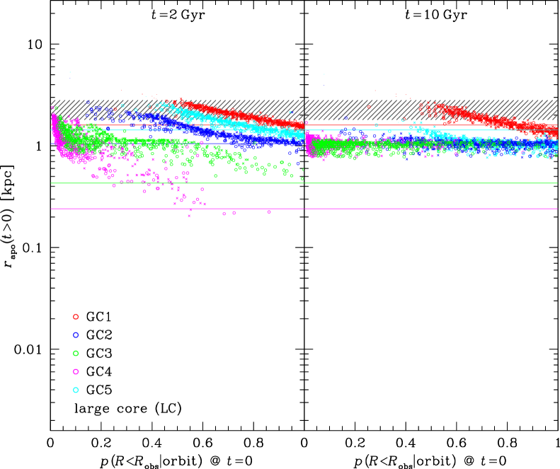
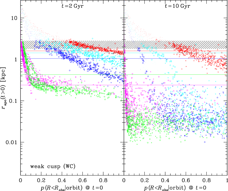
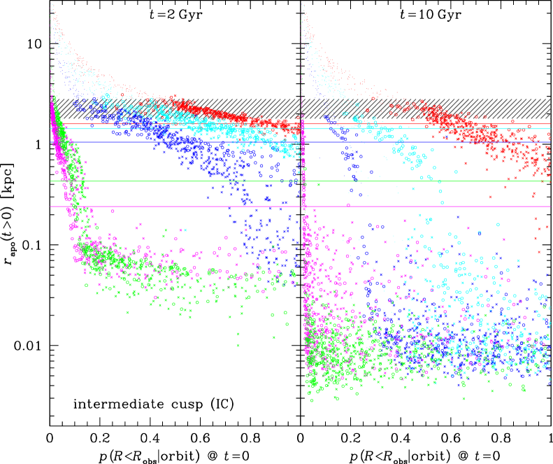
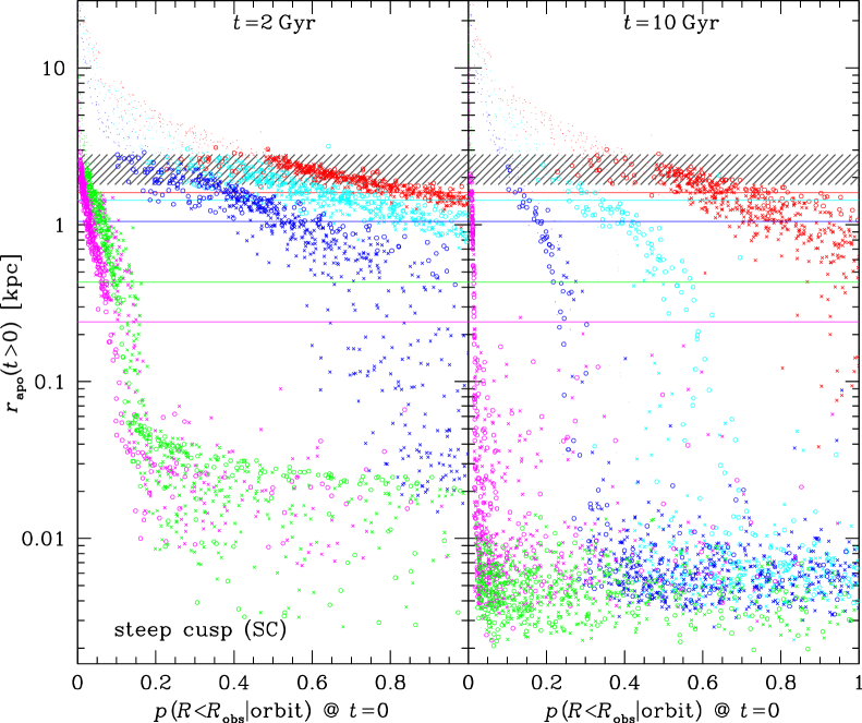
Figure 7: Instantaneous apo-centric radius $r_{\mathrm{apo}}$ at $t=2$ and 10 Gyr (as in Fig. 4) for all simulated clusters in a given halo model (as indicated) plotted versus the fraction $p(R\leq R_{\mathrm{p}}|\mathrm{orbit})$ of orbital phases and projections for which $R\leq R_{\mathrm{p}}$ on the initial cluster orbit. A uniform distribution of $p(R\leq R_{\mathrm{p}}|\mathrm{orbit})\in[0,1]$ corresponds to an unbiased distribution of orbital phases and projection angles. Dots are for orbits with initial $r_{\mathrm{apo}}>2.8\,$kpc, crosses for eccentricity $e>0.4$ and circles for $e<0.4$. The horizontal lines indicate $R_{\mathrm{p}}$ and the shaded band indicates the estimates for Fornax’s tidal radius.

5 The probability of cluster sinking

Our results presented in the previous Section and Fig. 4 demonstrate that the more massive clusters GC3 and GC4 will fall into the core of Fornax within 2 Gyr or less, unless either the mass distribution of Fornax has a core or the cluster has an initial orbit with large apo-centric radius $r_{\mathrm{apo}}$. This latter scenario requires that the observed cluster position is either near peri-centre (special orbital phase) or has intrinsic radius much larger than projected (special projection geometry). Either is atypical, implying that this scenario is inherently unlikely. In this section we try to quantify just how unlikely.

Since we know neither the current orbital phase nor projection geometry for any of the globular clusters, our most sensible approach is to marginalise over both, assuming uniform distributions. However, as we will see, our sampling of initial cluster position and velocity did not generate a uniform sampling in these quantities. As a consequence, any quantitative statements, based on the raw results, about the probability of cluster infall will be biased. In order to eliminate this bias, we must emulate a uniform sampling of initial orbital phases and projection geometries.

To this end, we need a quantity for each simulated cluster which would follow a known distribution were orbital phase and projection angle drawn randomly. A natural such quantity is the fraction

$$p(R\leq R_{\mathrm{p}}|\mathrm{orbit})$$

of orbital phases and projection geometries for which the projected radius $R$ is smaller than actually observed for the corresponding initial cluster orbit (see Appendix B for a formula and its derivation). Under our basic assumption of random orbital phase and projection, $p(R\leq R_{\mathrm{p}}|\mathrm{orbit})$ is uniformly distributed between 0 and 1, in particular $p(R\leq 0|\mathrm{orbit})=0$ and $p(R\leq r_{\mathrm{apo}}|\mathrm{orbit})=1$. We can therefore emulate a uniform distribution in orbital phase and projection geometry by a uniform distribution in $p(R\leq R_{\mathrm{p}}|\mathrm{orbit})$.

In Fig. 7, we plot for each simulated cluster and each halo mass model the instantaneous apo-centric radius $r_{\mathrm{apo}}$ after 2 and 10 Gyr against $p(R\leq R_{\mathrm{p}}|\mathrm{orbit})$. For all mass models, there is a clear correlation between $p(R\leq R_{\mathrm{p}}|\mathrm{orbit})$ and $r_{\mathrm{apo}}$ at later times in the sense that larger $r_{\mathrm{apo}}(t>0)$ are achieved only when the initial projected radius was relatively small for the initial orbit. This makes perfect sense: for small $p(R\leq R_{\mathrm{p}}|\mathrm{orbit})$ the orbit spends most of its time at $r>R_{\mathrm{p}}$ with little dynamical friction.

What is somewhat surprising, however, is how strong the correlation between $p(R\leq R_{\mathrm{p}}|\mathrm{orbit})$ and $r_{\mathrm{apo}}(t>0)$ actually is, given that the initial orbits cover a wide range of eccentricities. For simulated clusters with initial $r_{\mathrm{apo}}<2.8\,$kpc, we have split their initial orbits into low and high eccentricity

$$e=\frac{r_{\mathrm{apo}}-r_{\mathrm{peri}}}{r_{\mathrm{apo}}+r_{\mathrm{peri}}}$$ (8)

with open symbols and crosses in Fig. 7 corresponding to $e<0.4$ and $e>0.4$, respectively. For the halo models IC and SC, we can see some differentiation between these two groups of initial orbits, in particular at $t=2\,$Gyr, in the sense one would expect: eccentric orbits obtain smaller $r_{\mathrm{apo}}$ (because they have smaller initial $r_{\mathrm{peri}}$ and hence suffer more dynamical friction) unless the observed $R$ was initially untypically small (when they spend most of their time at large radii).

As is evident from Fig. 7, the distributions of $p(R\leq R_{\mathrm{p}}|\mathrm{orbit})$ from our simulations are not uniform: there are many more simulations with small $p(R\leq R_{\mathrm{p}}|\mathrm{orbit})$, in particular for clusters with small $R_{\mathrm{p}}$, such as GC3 and GC4. This non-uniformity is simply a consequence of our sampling procedure, which favours orbits with $r_{\mathrm{apo}}\gg R_{\mathrm{p}}$ (in particular for clusters with small $R_{\mathrm{p}}$, such as GC3 and GC4) resulting in non-uniform sampling of orbital phase and projection geometry and hence introducing a bias.

Since $r_{\mathrm{apo}}(t>0)$ is strongly correlated with $p(R\leq R_{\mathrm{p}}|\mathrm{orbit})$, we can read off Fig. 7 the unbiased probabilities for infall into Fornax. For example, in model SC $r_{\mathrm{apo}}(t=2\,\mathrm{Gyr})>200\,$pc for GC4 (magenta) in almost all simulations with $p(R\leq R_{\mathrm{p}}|\mathrm{orbit})<0.1$ but hardly for any simulation at larger $p(R\leq R_{\mathrm{p}}|\mathrm{orbit})$, implying that cluster GC4 will have $r_{\mathrm{apo}}>200\,$pc after 2Gyr with $\sim 10\%$ probability in halo model SC.

A more quantitative procedure for removing the bias of our non-uniform sampling of orbital phase and projection is to give each simulated cluster orbit a weight such that the weighed distributions of simulated orbits have, or at least are consistent with, a uniform sampling. Obviously, the weight to choose is simply the reciproce of the actual frequency $f\big{(}p(R\leq R_{\mathrm{p}}|\mathrm{orbit})\big{)}$ of fractions $p(R\leq R_{\mathrm{p}}|\mathrm{orbit})$ for all simulations of the same cluster in a particular halo model. The probability for, say $r_{\mathrm{apo}}(t=2\,\mathrm{Gyr})>200\,$pc for GC4, is then obtained as the weighted fraction of simulations that obtain $r_{\mathrm{apo}}(t=2\,\mathrm{Gyr})>200\,$pc for this cluster.

	any $e$			$e<0.4$			$e>0.4$
model	1 Gyr	2 Gyr	10 Gyr	1 Gyr	2 Gyr	10 Gyr	1 Gyr	2 Gyr	10 Gyr
	probability for no cluster with $r_{\mathrm{apo}}<100\,$pc
WC	1	1	$<$0.001	1	1	$<$0.001	1	1	$<$0.001
IC	0.17	0.032	$<$0.001	0.15	0.022	$<$0.001	0.19	0.037	$<$0.001
SC	0.10	0.017	$<$0.001	0.082	0.014	$<$0.001	0.11	0.020	$<$0.001
	probability for no cluster with $r_{\mathrm{apo}}<200\,$pc
WC	0.92	0.32	$<$0.001	0.87	0.29	$<$0.001	0.97	0.37	$<$0.001
IC	0.087	0.015	$<$0.001	0.049	0.011	$<$0.001	0.11	0.018	$<$0.001
SC	0.076	0.014	$<$0.001	0.063	0.011	$<$0.001	0.086	0.015	$<$0.001

Table 3: Probability, estimated as the fraction of orbital phases and projection geometries (consistent with the observed projected cluster positions) that no cluster with initial $r_{\mathrm{apo}}<2.8\,$kpc (Fornax’s tidal radius) has reached $r_{\mathrm{apo}}<100\,$pc or $200\,$pc after 1, 2, or 10 Gyr of simulation, depending on the mass model and the eccentricity of the initial orbit.

Combining this for all clusters, we estimate the probability that none of the five cluster when initially on orbit with $r_{\mathrm{apo}}<2.8\,$kpc (our upper limit for the tidal radius of Fornax) will fall into Fornax, in the sense that $r_{\mathrm{apo}}<100\,$pc or $<200\,$pc, within 1, 2, or 10 Gyr. The results for each halo model are given in Table 3 (except for model LC when no cluster ever falls into Fornax). Columns 2-4 give the probabilities based on all of our simulations. If we restrict the analysis to high or low eccentricities (columns 5-7 and 8-10, respectively) or to orbits with initial $r_{\mathrm{apo}}<1.8\,$kpc (not given in Table 3), the results are hardly altered.

In other words: these probabilities depend mainly on the halo model and only weakly on the distribution function of the cluster orbits. This is a direct consequence of the tight relation, seen in Fig. 7, between $p(R\leq R_{\mathrm{p}}|\mathrm{orbit})$ and $r_{\mathrm{apo}}$ at later times. This result implies that we do not need to investigate further the implications of different distributions functions for the initial cluster orbits.

6 Conclusions

The Fornax galaxy is unique among the Milky Way dSphs in having five surviving globular clusters. These clusters are metal poor and very old – comparable with the oldest globular clusters in the Milky Way. There is a well-known timing problem for these clusters: over a Hubble time or even a much shorter time scale dynamical friction should drag them to the centre of Fornax, where they would form a nuclear star cluster. Yet no such stellar nucleus is observed in Fornax or, in fact, in any other dSph galaxy.

In this study, we have extended previous work on what the current location of Fornax’s globular clusters can tell us about Fornax’s mass distribution. We explored four different mass models for the underlying potential in Fornax; we used the latest data for Fornax’s globular clusters as constraints on their phase space distribution; and we ran thousands of $N$-body models to sample the uncertainties in the cluster position and velocity distribution for each of our five mass models. This large search of the available parameter space allowed us to hunt for viable solutions to Fornax’s timing problem.

6.1 Caveats

Our models all assume a spherical mass distribution for Fornax, yet the stars are observed to be ellipsoidal in projection, implying that the true intrinsic distribution is aspherical, most likely triaxial. The parameter space of such configurations is considerably larger (and the freedom in cluster orbital projections smaller), potentially allowing more solutions to the timing problem. However, previous studies suggest that, while dynamical friction is on average stronger on box orbits than on loop orbits(Capuzzo-Dolcetta & Vicari, 2005), triaxiality has no sifnificant overall effect on the strength of dynamical friction (Cora, Vergne & Muzzio, 2001; Sachania, 2009). This can be understood as cancellation of two opposing effects. First, because angular momentum is not conserved, there is no barrier for eccentric orbits to reach arbitrary small radii and hence high densities and strong drag. Second, also because angular momentum is not conserved, successive peri-centric passages have different radius and density, such that an orbiting cluster only rarely suffers very high drags.

Another minor caveat of our modelling is our ignorance of the tidal field of the Milky-Way potential. In principle, it would be trivial to have our $N$-body models orbit in a static model for the Galactic potential. However, such a procedure would add even more only weakly constrained parameters without adding significant benefits. With our existing models, we take the Galactic tidal effects into account by discounting any simulated cluster orbits with apo-centric radius beyond (best estimates of) Fornax’s tidal radius.

Finally, by modelling each globular cluster as a massive particle, we have ignored their inner dynamics and tidal interaction with Fornax. Mass-loss rates for these clusters, however, are likely to be too small to significantly reduce their mass (Goerdt et al., 2010). Tidal disruption is arguably only relevant for GC1, as discussed in §6.3 below.

6.2 Solutions to the timing problem

Our simulations demonstrate that for normal mass models (WC, IC, or SC) for Fornax the infall of clusters GC3 and GC4 within a Hubble time is unavoidable and the infall of all clusters except GC1 most likely. This constitutes the long-term timing problem in the sense of hypothesis 1 from page 1, which is only really a problem if one assumes that the present globular cluster distribution of Fornax is representative of the distant past.

Only our large-core model (LC) avoids this problem completely. Rather than dynamical friction, this model shows ‘dynamical buoyancy’, when clusters are pushed out of the core. Following Tremaine & Weinberg (1984), this is likely caused by this model’s inverted distribution function, when $\mathop{}\!\mathrm{d}f/\mathop{}\!\mathrm{d}E>0$ over a significant range of orbital energies $E$. Such models are generally thought to be unstable (Binney & Tremaine, 2008, §5.5). Hence, it seems unlikely that such a model emerges from any reasonable formation mechanism. However, our $N$-body models appears to be stable, and some further research is needed to clarify the cause for ‘dynamical buoyancy’, its relation to the core stalling effect (reported by Read et al., 2006), and its prospects in natural systems.

For cusped mass models (IC & SC), such as predicted by CDM cosmogony via dissipationless simulations, clusters GC3 or GC4 will sink into the centre of Fornax within 1-2 Gyr with $\sim 90\%$ probability (in the sense that solutions where this does not occur cover only $\sim 10\%$ of the possible orbital phases and projections). In fact, we estimate the probability that no cluster obtains $r_{\mathrm{apo}}\lesssim 100\,$pc within 2 Gyr to be no more than 2% in Table 3. This is largely independent of the assumed globular-cluster orbital distribution function and constitues the more severe immediate timing problem in the sense of hypothesis 2 from page 1. It implies that if Fornax indeed has a cusped density profile, our cosmic epoch of observation is necessarily very special.

For a shallow cusp model (WC), only the most massive cluster GC3 has a 90% probability to reach, within 1–2 Gyr, $r_{\mathrm{apo}}\lesssim 200\,$pc significantly less than its current projected radius of $R_{\mathrm{p}}=430\,$pc. For this model, no cluster can reach $r_{\mathrm{apo}}\lesssim 100\,$pc within 2 Gyr and the chances that no cluster will reach $r_{\mathrm{apo}}\lesssim 200\,$pc within 1 or 2 Gyr are, respectively, 92% and 32% (see Table 3). These numbers are not unlikely and hence avoid the long-term timing problem.

6.2.1 A steady-state solution

Our finding thus suggest two possible solutions to the timing problem. First, Fornax has a large core (perhaps between models LC and WC) and dynamical friction is slow or has stalled a long time ago. In this case, Fornax may have been on its current orbit for a Hubble time with its globular cluster system hardly evolving. In this case, the consistency of the cluster distribution with the stellar distribution (as discussed in §2.2) cannot be a coincidence, but hints at a common formation scenario.

6.2.2 An evolving solution

In the second solution Fornax has a small core or shallow cusp (as model WC) and dynamical friction is still ongoing, albeit slowly enough that the absence of a central nucleus in Fornax (or in fact any other dSph) is perfectly plausible. In this case, the clusters must have been further away from Fornax in the past than today, and the current (weak) consistency of their distribution with that of the stars is just a coincidence. Also, a Hubble time ago the clusters most likely were more than the current tidal radius of 1.8–2.8 kpc away from Fornax. This in turn requires Fornax did not orbit the Milky Way for a Hubble time on its present orbit. However, even a simple adiabatic evolution of Fornax’s orbit may be sufficient to solve this problem. For example, for a slowly growing Galaxy with always flat rotation curve the peri-centric tidal radius of Fornax evolves like $r_{\mathrm{tid}}\propto\upsilon_{\mathrm{circ}}^{-4/3}$ (even when neglecting mass-loss of Fornax due to Galactic tides).

This second solution appears more natural and also fits with the weak indication of mass-segregation, as would be induced by dynamical friction, in the current mass-radius relation (see Fig. 1). However, this model implies that the globular clusters have not formed within Fornax, but are most likely accreted. One may, of course, consider these two solutions as the extreme ends of a continuity of solutions with various degrees of cusp strengths and hence dynamical friction effects.

6.3 The case of GC1

An interesting aspect relates to the cluster GC1. Peñarrubia, Walker & Gilmore (2009) demonstrated that, uniquely of all Fornax’s globular clusters, GC1 would be tidally disrupted if it fell to the centre of Fornax. While we find that GC1 does not sink to the centre of Fornax in almost all of our models, this still leaves us with a puzzle. Why should the one cluster vulnerable to tides be on an orbit where it would hardly ever suffer disruption? For our steady-state solution to the timing problem above, this puzzle can be resolved by the postulation that Fornax once had a richer globular-cluster system and we only see the survivors. Such survivors are either massive enough or on remote orbits to avoid tidal disruption. However, a high (initial) frequency of globular clusters (of $\sim 10^{4-5}\mbox{M${}_{\odot}$}$) appears rather implausible for a small galaxy like Fornax.

For the evolving solution to the timing problem, on the other hand, the fact that GC1 would be disrupted poses no problem at all. In this picture, low-mass clusters, such as GC1, would not be dragged down much, and there is no need to postulate a large early population of clusters.

Appendix A Numerical convergence

In order to ensure that our simulations do not suffer from numerical noise we ran simulations with two different mass models, one cusped and one cored; each with two different orbits, one circular and one eccentric; and each of these at three different resolutions: with $N=4\times 10^{5}$, $10^{6}$ and $4\times 10^{6}$. We then compared the evolution in each case of one cluster over 10 Gyr.

The evolution of the orbital radius of a single cluster moving on an eccentric orbit in model WC (see table 2) is shown in Fig. 8. It can be seen that orbital evolution is very similar for all resolutions. In particular, the decay of the orbit follows the same timescale, with the time and radius of the first-stalling of the cluster being the same. It has been shown that the two-body noise in a simulation can cause the cluster orbit to precess and cause artificial decay of the orbit once in the core (Read et al., 2006). We selected the above combination of orbit and density profile precisely because Read et al. (2006) showed that convergence is most difficult for an eccentric orbit in a cored halo. This is the case where numerical friction caused by orbit precession has the largest effect on orbital decay. The simulations shown above give a strong indication that such effects are not significant at even lower resolutions than the one used for the main body of this work. Our simulations are well converged.

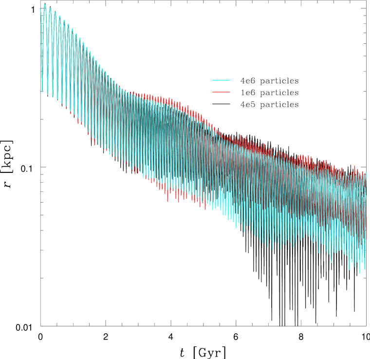
Figure 8: The evolution of the radius for a single cluster moving on an eccentric orbit in a halo with a near-cored density profile (model WC from Table 2), but realised with different particle numbers as indicated. Some of the deviation at later times is due to the uncertainties in determining the centre of the $N$-body model.

Appendix B The probability for $R\leq R_{\mathrm{p}}$

The fraction of orbital phases and projections for which $R\leq R_{\mathrm{p}}$ on a given orbit is identical to the probability for $R\leq R_{\mathrm{p}}$, when $R$ is computed for that orbit at random orbital phase and projection.

The probability for a cluster with orbital energy $E$ and angular momentum $L$ to be found at a radius between $r$ and $r+dr$ is

$$p(r|E,L)\,\mathop{}\!\mathrm{d}r=\frac{2\,\mathop{}\!\mathrm{d}r}{T_{r}\,\upsilon_{r}}\qquad\qquad\text{if}\;r_{\mathrm{peri}}\leq r\leq r_{\mathrm{apo}}$$ (9)

and zero otherwise. $r_{\mathrm{peri}}\leq r_{\mathrm{apo}}$ are the roots of the radial velocity

$$\upsilon_{r}^{2}=2\left[E-\Phi(r)\right]-L^{2}/r^{2},$$ (10)

and the radial period is given by

$$T_{r}=2\int_{r_{\mathrm{peri}}}^{r_{\mathrm{apo}}}\frac{\mathop{}\!\mathrm{d}r}{\upsilon_{r}}.$$ (11)

The probability that a cluster at radius $r$ has projected radius between $R$ and $R+\mathop{}\!\mathrm{d}R$ is

$$p(R|r)\,\mathop{}\!\mathrm{d}R=\frac{R\,\mathop{}\!\mathrm{d}R}{r\sqrt{r^{2}-R^{2}}}\qquad\qquad\text{if}\;R\leq r$$ (12)

and zero otherwise. Thus, the probability for a cluster with given orbit to have projected radius between $R$ and $R+\mathop{}\!\mathrm{d}R$ is

$$p(R|E,L)\,\mathop{}\!\mathrm{d}R=\mathop{}\!\mathrm{d}R\int_{\max\{R,r_{\mathrm{peri}}\}}^{r_{\mathrm{apo}}}p(R|r)\,p(r|E,L)\,\mathop{}\!\mathrm{d}r$$ (13)

for $R\leq r_{\mathrm{apo}}$ and zero otherwise. From this, we can work out the finite probability that a cluster with given orbit has projected radius not greater than observed:

$$p(R\leq R_{\mathrm{p}}|E,L) = \int_{0}^{R_{\mathrm{p}}}p(R|E,L)\,\mathop{}\!\mathrm{d}R$$ (14)

$$= \frac{2}{T_{r}}\int_{0}^{R_{\mathrm{p}}}\mathop{}\!\mathrm{d}R\int_{\max\{R,r_{\mathrm{peri}}\}}^{r_{\mathrm{apo}}}\frac{R}{r\sqrt{r^{2}-R^{2}}}\frac{\mathop{}\!\mathrm{d}r}{\upsilon_{r}}$$

$$= \frac{2}{T_{r}}\int_{r_{\mathrm{peri}}}^{r_{\mathrm{apo}}}\frac{\mathop{}\!\mathrm{d}r}{\upsilon_{r}}\int_{0}^{\min\{r,R_{\mathrm{p}}\}}\frac{R\mathop{}\!\mathrm{d}R}{r\sqrt{r^{2}-R^{2}}}$$

$$= \int_{r_{\mathrm{peri}}}^{r_{\mathrm{apo}}}\left[1-(1-R_{\mathrm{p}}^{2}/r^{2})_{+}^{1/2}\right]\frac{\mathop{}\!\mathrm{d}r}{\upsilon_{r}}\Bigg{/}\int_{r_{\mathrm{peri}}}^{r_{\mathrm{apo}}}\frac{\mathop{}\!\mathrm{d}r}{\upsilon_{r}}.$$

with $(\cdot)_{+}\equiv\max\{0,\cdot\}$. One can easily verify that $p(R\leq 0|E,L)=0$ and $p(R\leq r_{\mathrm{apo}}|E,L)=1$, as required.

References

- Amorisco & Evans (2011a) Amorisco N. C., Evans N. W., 2011a, MNRAS, p. 1606
- Amorisco & Evans (2011b) Amorisco N. C., Evans N. W., 2011b, MNRAS, 411, 2118
- Angus & Diaferio (2009) Angus G. W., Diaferio A., 2009, MNRAS, 396, 887
- Battaglia et al. (2008) Battaglia G., Helmi A., Tolstoy E., Irwin M., Hill V., Jablonka P., 2008, ApJ, 681, L13
- Binney & Tremaine (2008) Binney J. J., Tremaine S., 2008, Galactic dynamics. 2nd ed. Princeton, NJ, Princeton University Press
- Breddels et al. (2012) Breddels M. A., Helmi A., van den Bosch R. C. E., van de Ven G., Battaglia G., 2012, preprint, arXiv:1205.4712
- Buonanno et al. (1999) Buonanno R., Corsi C. E., Castellani M., Marconi G., Fusi Pecci F., Zinn R., 1999, AJ, 118, 1671
- Buonanno et al. (1998) Buonanno R., Corsi C. E., Zinn R., Fusi Pecci F., Hardy E., Suntzeff N. B., 1998, ApJ, 501, L33
- Capuzzo-Dolcetta & Vicari (2005) Capuzzo-Dolcetta R., Vicari A., 2005, MNRAS, 356, 899
- Cole et al. (2011) Cole D. R., Dehnen W., Wilkinson M. I., 2011, MNRAS, 416, 1118
- Coleman et al. (2004) Coleman M., Da Costa G. S., Bland-Hawthorn J., Martínez-Delgado D., Freeman K. C., Malin D., 2004, AJ, 127, 832
- Coleman et al. (2005) Coleman M. G., Da Costa G. S., Bland-Hawthorn J., Freeman K. C., 2005, AJ, 129, 1443
- Cora et al. (2001) Cora S. A., Vergne M. M., Muzzio J. C., 2001, ApJ, 546, 165
- Dehnen (2000) Dehnen W., 2000, ApJ, 536, L39
- Dehnen (2002) Dehnen W., 2002, J. Comp. Phys., 179, 27
- Dinescu et al. (2004) Dinescu D. I., Keeney B. A., Majewski S. R., Girard T. M., 2004, AJ, 128, 687
- Dubinski & Carlberg (1991) Dubinski J., Carlberg R. G., 1991, ApJ, 378, 496
- El-Zant et al. (2001) El-Zant A., Shlosman I., Hoffman Y., 2001, ApJ, 560, 636
- Elson et al. (1987) Elson R. A. W., Fall S. M., Freeman K. C., 1987, ApJ, 323, 54
- Gerhard (1991) Gerhard O. E., 1991, MNRAS, 250, 812
- Gilmore et al. (2007) Gilmore G., Wilkinson M. I., Wyse R. F. G., Kleyna J. T., Koch A., Evans N. W., Grebel E. K., 2007, ApJ, 663, 948
- Goerdt et al. (2010) Goerdt T., Moore B., Read J. I., Stadel J., 2010, ApJ, 725, 1707
- Goerdt et al. (2006) Goerdt T., Moore B., Read J. I., Stadel J., Zemp M., 2006, MNRAS, 368, 1073
- Greco et al. (2007) Greco C., Clementini G., Catelan M., Held E. V., Poretti E., Gullieuszik M., Maio M., Rest A., De Lee N., Smith H. A., Pritzl B. J., 2007, ApJ, 670, 332
- Hernquist (1990) Hernquist L., 1990, ApJ, 356, 359
- Hogan & Dalcanton (2000) Hogan C. J., Dalcanton J. J., 2000, Phys. Rev. D, 62, 063511
- Inoue (2009) Inoue S., 2009, MNRAS, 397, 709
- King (1962) King I., 1962, AJ, 67, 274
- Kleyna et al. (2002) Kleyna J., Wilkinson M. I., Evans N. W., Gilmore G., Frayn C., 2002, MNRAS, 330, 792
- Kleyna et al. (2003) Kleyna J. T., Wilkinson M. I., Gilmore G., Evans N. W., 2003, ApJ, 588, L21
- Kochanek & White (2000) Kochanek C. S., White M., 2000, ApJ, 543, 514
- Łokas (2009) Łokas E. L., 2009, MNRAS, 394, L102
- Lux et al. (2010) Lux H., Read J. I., Lake G., 2010, MNRAS, 406, 2312
- Maccio’ et al. (2012) Maccio’ A. V., Paduroiu S., Anderhalden D., Schneider A., Moore B., 2012, preprint, arXiv:1202.1282
- Mackey & Gilmore (2003a) Mackey A. D., Gilmore G. F., 2003a, MNRAS, 343, 747
- Mackey & Gilmore (2003b) Mackey A. D., Gilmore G. F., 2003b, MNRAS, 340, 175
- Mateo et al. (1991) Mateo M., Olszewski E., Welch D. L., Fischer P., Kunkel W., 1991, AJ, 102, 914
- Mateo (1998) Mateo M. L., 1998, ARA&A, 36, 435
- Navarro et al. (1996) Navarro J. F., Eke V. R., Frenk C. S., 1996, MNRAS, 283, L72
- Navarro et al. (1996) Navarro J. F., Frenk C. S., White S. D. M., 1996, ApJ, 462, 563
- Oh et al. (2000) Oh K. S., Lin D. N. C., Richer H. B., 2000, ApJ, 531, 727
- Peñarrubia et al. (2008) Peñarrubia J., McConnachie A. W., Navarro J. F., 2008, ApJ, 672, 904
- Peñarrubia et al. (2009) Peñarrubia J., Walker M. G., Gilmore G., 2009, MNRAS, 399, 1275
- Plummer (1911) Plummer H. C., 1911, MNRAS, 71, 460
- Pontzen & Governato (2012) Pontzen A., Governato F., 2012, MNRAS, 421, 3464
- Read & Gilmore (2005) Read J. I., Gilmore G., 2005, MNRAS, 356, 107
- Read et al. (2006) Read J. I., Goerdt T., Moore B., Pontzen A. P., Stadel J., Lake G., 2006, MNRAS, 373, 1451
- Read et al. (2006) Read J. I., Wilkinson M. I., Evans N. W., Gilmore G., Kleyna J. T., 2006, MNRAS, 366, 429
- Sachania (2009) Sachania J., 2009, PhD thesis, University of Leicester, Leicester, UK
- Saha (1992) Saha P., 1992, MNRAS, 254, 132
- Sánchez-Salcedo et al. (2006) Sánchez-Salcedo F. J., Reyes-Iturbide J., Hernandez X., 2006, MNRAS, 370, 1829
- Strigari et al. (2006) Strigari L. E., Bullock J. S., Kaplinghat M., Kravtsov A. V., Gnedin O. Y., Abazajian K., Klypin A. A., 2006, ApJ, 652, 306
- Strigari et al. (2008) Strigari L. E., Bullock J. S., Kaplinghat M., Simon J. D., Geha M., Willman B., Walker M. G., 2008, Nature, 454, 1096
- Tremaine & Gunn (1979) Tremaine S., Gunn J. E., 1979, Physical Review Letters, 42, 407
- Tremaine & Weinberg (1984) Tremaine S., Weinberg M. D., 1984, MNRAS, 209, 729
- Tremaine (1976) Tremaine S. D., 1976, ApJ, 203, 345
- Tremaine et al. (1975) Tremaine S. D., Ostriker J. P., Spitzer Jr. L., 1975, ApJ, 196, 407
- Villaescusa-Navarro & Dalal (2011) Villaescusa-Navarro F., Dalal N., 2011, J. Cosm. & Astroparticle Phys., 3, 24
- Walker et al. (2007) Walker M. G., Mateo M., Olszewski E. W., Gnedin O. Y., Wang X., Sen B., Woodroofe M., 2007, ApJ, 667, L53
- Walker et al. (2009) Walker M. G., Mateo M., Olszewski E. W., Peñarrubia J., Wyn Evans N., Gilmore G., 2009, ApJ, 704, 1274
- Walker & Peñarrubia (2011) Walker M. G., Peñarrubia J., 2011, ApJ, 742, 20
- Wilkinson et al. (2002) Wilkinson M. I., Kleyna J., Evans N. W., Gilmore G., 2002, MNRAS, 330, 778