A Framework for Evaluating Approximation Methods for Gaussian Process Regression

Abstract

Gaussian process (GP) predictors are an important component of many Bayesian approaches to machine learning. However, even a straightforward implementation of Gaussian process regression (GPR) requires $O(n^{2})$ space and $O(n^{3})$ time for a dataset of $n$ examples. Several approximation methods have been proposed, but there is a lack of understanding of the relative merits of the different approximations, and in what situations they are most useful. We recommend assessing the quality of the predictions obtained as a function of the compute time taken, and comparing to standard baselines (e.g., Subset of Data and FITC). We empirically investigate four different approximation algorithms on four different prediction problems, and make our code available to encourage future comparisons.

Keywords: Gaussian process regression, subset of data, FITC, local GP.

Gaussian process (GP) predictors are widely used in non-parametric Bayesian approaches to supervised learning problems (Rasmussen and Williams, 2006). They can also be used as components for other tasks including unsupervised learning (Lawrence, 2004), and dependent processes for a variety of applications (e.g., Sudderth and Jordan 2009; Adams et al. 2010). The basic model on which these are based is Gaussian process regression (GPR), for which a standard implementation requires $O(n^{2})$ space and $O(n^{3})$ time for a dataset of $n$ examples, see e.g. Rasmussen and Williams (2006, ch. 2). Several approximation methods have now been proposed, as detailed below. Typically the approximation methods are compared to the basic GPR algorithm. However, as there are now a range of different approximations, the user is faced with the problem of understanding their relative merits, and in what situations they are most useful.

Most approximation algorithms have a tunable complexity parameter, which we denote as $m$. Our key recommendation is to study the quality of the predictions obtained as a function of the compute time taken as $m$ is varied, as times can be compared across different methods. New approximation methods should be compared against current baselines like Subset of Data and FITC (described in Secs. 1.1–1.2). The time decomposes into that needed for training the predictor (including setting hyperparameters), and test time; the user needs to understand which will dominate in their application. We illustrate this process by studying four different approximation algorithms on four different prediction problems. We have published our code in order to encourage comparisons of other methods against these baselines.

The structure of the paper is as follows: In Section 1 we outline the complexity of the full GP algorithm and various approximations, and give some specific details needed to apply them in practice. Section 2 outlines issues that should be considered when selecting or developing a GP approximation algorithm. Section 3 describes the experimental setup for comparisons, and the results of these experiments. We conclude with future directions and a discussion.

1 Approximation algorithms for Gaussian Process Regression (GPR)

A regression task has a training set ${\cal D}\!=\!\{\mathbf{x}_{i},y_{i}\}_{i=1}^{n}$ with $D$-dimensional inputs $\mathbf{x}_{i}$ and scalar outputs $y_{i}$. Assuming that the outputs are noisy observations of a latent function $f$ at values $f_{i}\!=\!f(\mathbf{x}_{i})$, the goal is to compute a predictive distribution over the latent function value $f_{*}$ at a test location $\mathbf{x}_{*}$.

Assuming a Gaussian process prior over functions $f$ with zero mean, and covariance or kernel function $k(\cdot,\cdot)$, and Gaussian observations, $y_{i}=f_{i}+\epsilon_{i}$ where $\epsilon_{i}\sim{\mathcal{N}}(0,\sigma^{2})$, gives Gaussian predictions $p(f_{*}\!\mid\!\mathbf{x}_{*},{\cal D})\!=\!{\mathcal{N}}(\overline{f}_{*},\mathbbm{V}[f_{*}])$, with predictive mean and variance (see e.g., Rasmussen and Williams, 2006, Sec. 2.2):

$$\overline{f}_{*} = \mathbf{k}^{\top}(\mathbf{x}_{*})(K+\sigma^{2}I)^{-1}\mathbf{y}\;\;{\stackrel{{\scriptstyle\mathit{def}}}{{=}}}\;\;\mathbf{k}^{\top}(\mathbf{x}_{*})\mbox{\boldmath{$\alpha$}},$$ (1)

$$\mathbbm{V}[f_{*}] = k(\mathbf{x}_{*},\mathbf{x}_{*})-\mathbf{k}^{\top}(\mathbf{x}_{*})(K+\sigma^{2}I)^{-1}\mathbf{k}(\mathbf{x}_{*}),$$ (2)

where $K$ is the $n\times n$ matrix with $K_{ij}=k(\mathbf{x}_{i},\mathbf{x}_{j})$, $\mathbf{k}(\mathbf{x}_{*})$ is the $n\times 1$ column vector with the $i$th entry being $k(\mathbf{x}_{*},\mathbf{x}_{i})$, $\mathbf{y}$ is the column vector of the $n$ target values, and $\mbox{\boldmath{$\alpha$}}=(K+\sigma^{2}I)^{-1}\mathbf{y}$.

The log marginal likelihood of the GPR model is also available in closed form:

$$L=\log p(\mathbf{y}|X)=-\tfrac{1}{2}\,\mathbf{y}^{\top}(K+\sigma^{2}_{n}I)^{-1}\mathbf{y}-\tfrac{1}{2}\log|K+\sigma^{2}I|-\tfrac{n}{2}\log 2\pi.$$ (3)

Typically $L$ is viewed as a function of a set of parameters $\theta$ that specify the kernel. Below we assume that $\theta$ is set by numerically maximizing $L$ with a routine like conjugate gradients. Computation of $L$ and the gradient $\nabla_{\theta}L$ can be carried out in $O(n^{3})$. Optimizing $L$ is a maximum-likelihood type II or ML-II procedure for $\theta$; alternatively one might sample over $p(\theta|{\cal D})$ using e.g. MCMC. Equations 1–3 form the basis of GPR prediction.

We identify three computational phases in carrying out GPR:

hyperparameter learning:

The hyperparameters are learned, by for example maximizing the log marginal likelihood. This is often the most computationally expensive phase.

training:

Given the hyperparameters, all computations that don’t involve test inputs are performed, such as computing $\alpha$ above, and/or computing the Cholesky decomposition of $K+\sigma^{2}_{n}I$. This phase was called “precomputation” by Quiñonero-Candela et al. (2007, Sec. 9.6).

testing:

Only the computations involving the test inputs are carried out, those which could not have been done previously. This phase may be significant if there is a very large test set, or if deploying a trained model on a machine with limited resources.

Table 1 lists the computational complexity of training and testing full GPR as a function of $n$. Evaluating the marginal likelihood $L$ and its gradient takes more operations than ‘training’ (i.e. computing the parts of (1) and (2) that don’t depend on $\mathbf{x}_{*}$), but has the same scaling with $n$. Hyperparameter learning involves evaluating $L$ for all values of the hyperparameters $\theta$ that are searched over, and so is more expensive than training for fixed hyperparameters.

Method	Storage	Training	Mean	Variance
Full	$O(n^{2})$	$O(n^{3})$	$O(n)$	$O(n^{2})$
SoD	$O(m^{2})$	$O(m^{3})$	$O(m)$	$O(m^{2})$
FITC	$O(mn)$	$O(m^{2}n)$	$O(m)$	$O(m^{2})$
Local	$O(mn)$	$O(m^{2}n)$	$O(m)$	$O(m^{2})$

Table 1: A comparison of the space and time complexity of the Full, SoD, FITC and Local methods, ignoring the time taken to select the $m$ subset/inducing points/clusters from the $n$ datapoints. Training: the time required for preliminary computations before the test point $\mathbf{x}_{*}$ is known, for each hyperparameter setting considered. Mean (resp. variance): the time needed to compute the predictive mean (variance) at test point $\mathbf{x}_{*}$.

These complexities can be reduced in special cases, e.g. for stationary covariance functions and grid designs, as may be found e.g. in geoscience problems. In this case the eigenvectors of $K$ are the Fourier basis, and matrix inversions etc can be computed analytically. See e.g. Wikle et al. (2001); Paciorek (2007); Fritz et al. (2009) for more details.

Common methods for approximate GPR include Subset of Data (SoD), where data points are simply thrown away; inducing point methods (Quiñonero-Candela and Rasmussen, 2005), where $K$ is approximated by a low-rank plus diagonal form; Local methods where nearby data is used to make predictions in a given region of space; and fast matrix-vector multiplication (MVM) methods, which can be used with iterative methods to speed up the solution of linear systems. We discuss these in turn, so as to give coverage to the wide variety methods that have been proposed. We use the Fully Independent Training Conditional (FITC) method as it is recommended over other inducing point methods in Quiñonero-Candela et al. (2007), and the Improved Fast Gauss Transform (IFGT) of Yang et al. (2005) as a representative of fast MVM methods.

1.1 Subset of Data

The simplest way of dealing with large amounts of data is simply to ignore some or most of it. The ‘Subset of Data (SoD) approximation’ simply applies the full GP prediction method to a subset of size $m<n$. Therefore the computational complexities of SoD result from replacing $n$ with $m$ in the expressions for the full method (Table 1). Despite the ‘obvious’ nature of SoD, most papers on approximate GP methods only compare to a GP applied to the full dataset of size $n$.

To complete the description of the SoD method we must also specify how the subset is selected. We consider two of the possible alternatives: 1) Selecting $m$ points randomly costs $O(m)$ if we need not look at the other points. 2) We select $m$ cluster centres from a Farthest Point Clustering (FPC, Gonzales 1985) of the dataset; using the algorithm proposed by Gonzales this has computational complexity of $O(mn)$. In theory, FPC can be sped up to $O(n\log m)$ using suitable data structures (Feder and Greene, 1988), although in practice the original algorithm can be faster for machine learning problems of moderate dimensionality. FPC has a random aspect as the first point can be chosen randomly. Our SoD implementation is based on gp.m in the Matlab gpml toolbox:
http://www.gaussianprocess.org/gpml/code/matlab/doc/.

Rather than selecting the subset randomly, it is also possible to make a more informed choice. For example Lawrence et al. (2003) came up with a fast selection scheme (the “informative vector machine”) that takes only $O(m^{2}n)$. Keerthi and Chu (2006) also proposed a matching pursuit approach which has similar asymptotic complexity, although the associated constant is larger.

1.2 Inducing point methods: FITC

A number of GP approximation algorithms use alternative kernel matrices based on inducing points, $\mathbf{u}$, in the $D$-dimensional input space (Quiñonero-Candela and Rasmussen, 2005). Here we restrict the $m$ inducing points to be a subset of the training inputs. The Subset of Regressors (SoR) kernel function is given by $k_{SoR}(\mathbf{x}_{i},\mathbf{x}_{j})=\mathbf{k}(\mathbf{x}_{i},\mathbf{u})K^{-1}_{\mathbf{u}\mathbf{u}}\mathbf{k}(\mathbf{u},\mathbf{x}_{j})$, and the Fully Independent Training Conditional (FITC) method uses

$$k_{FITC}(\mathbf{x}_{i},\mathbf{x}_{j})=k_{SoR}(\mathbf{x}_{i},\mathbf{x}_{j})+\delta_{ij}[k(\mathbf{x}_{i},\mathbf{x}_{j})-k_{SoR}(\mathbf{x}_{i},\mathbf{x}_{j})].$$

FITC approximates the matrix $K$ as a rank-$m$ plus diagonal matrix. An attractive property of FITC, not shared by all approximations, is that it corresponds to exact inference for a GP with the given $k_{FITC}$ kernel (Quiñonero-Candela et al., 2007). Other inducing point approximations (e.g. SoR, deterministic training conditionals) have similar complexity but Quiñonero-Candela et al. (2007) recommend FITC over them. Since then there have been further developments (Titsias, 2009; Lázaro-Gredilla et al., 2010), which would also be interesting to compare.

To make predictions with FITC, and to evaluate its marginal likelihood, simply substitute $k_{FITC}$ for the original kernel in Equations 1–3. This substitution gives a mean predictor of the form $\overline{f}_{*}=\sum_{i=1}^{m}\beta_{i}k(\mathbf{x}_{*},\mathbf{x}_{i})$, where $i=1,\ldots,m$ indexes the selected subset of training points, and the $\beta$s are obtained by solving a linear system. Snelson (2007, pp 60-62) showed that in the limit of zero noise FITC reduces to SoD.

We again choose a set of inducing points of size $m$ from the training inputs either randomly or using FPC, and use the FITC implementation from the gpml toolbox.

It is possible to “mix and match” the SoD and FITC methods, adapting the hyperparmeters to optimize the SoD approximation to the marginal likelihood, then using the FITC algorithm to make predictions using the same data subset and the SoD-trained hyperparameters. We refer to this procedure as the Hybrid method. We expect that saving time on the hyperparameter learning phase, $O(m^{3})$ instead of $O(m^{2}n)$, will come at the cost of reducing the predictive performance of FITC for a given $m$.

1.3 Local GPR

The basic idea here is of divide-and-conquer, although without any guarantees of correctness. We divide the $n$ training points into $k=\lceil\frac{n}{m}\rceil$ clusters each of size $m$, and run GPR in each cluster, ignoring the training data outside of the given cluster. At test time we assign a test input $\mathbf{x}_{*}$ to the closest cluster. This method has been discussed by Snelson and Ghahramani (2007). The hard cluster boundaries can lead to ugly discontinuities in the predictions, which are unacceptable if a smooth surface is required, for example in some physical simulations.

One important issue is how the clustering is done. We found that FPC tended to produce clusters of very unequal size, which limited the speedups obtained by Local GPR. Thus we devised a method we call Recursive Projection Clustering (RPC), which works as follows. We start off with all the data in one cluster $C$. Choose two data points at random from $C$, draw a line through these points and calculate the orthogonal projection of all points from $C$ onto the line. Split $C$ into two equal-sized subsets $C_{L}$ and $C_{R}$ depending on whether points are to the left or right of the median. Now repeat recursively in each cluster until the cluster size is no larger than $m$. In our implementation we make use of Matlab’s sort function to find the median value, taking time $O(n\log n)$ for $n$ datapoints, although it is possible to reduce median finding to $O(n)$ (Blum et al., 1973). Thus overall the complexity of RPC is $O(ns\log n)$, where $s=\lceil\log_{2}(n/m)\rceil$. A test point $\mathbf{x}_{*}$ is assigned to the appropriate cluster by descending the tree of splits constructed by RPC.

Another issue concerns hyperparameter learning. $L$ is approximated by the sum of terms like Eq. 3 over all clusters. Hyperparameters can either be tied across all clusters (“joint” training), or unique to each cluster (“separate” training). Joint training is likely to be useful for small $m$. We implemented Local GPR using the gpml toolbox with small modifications to sum gradients for joint training.

1.4 Iterative methods and IFGT matrix-vector multiplies

The Conjugate Gradients (CG) method (e.g., Golub and Van Loan 1996) can be used at training time to solve the linear system $(K+\sigma^{2}I)\mbox{\boldmath{$\alpha$}}=\mathbf{y}$. Indeed, all GPR computations can be based on iterative methods (Gibbs, 1997). CG and several other iterative methods (e.g., Li et al. 2007; Liberty et al. 2007) for solving linear systems require the ability to multiply a matrix of kernel values with an arbitrary vector.

Standard dense matrix-vector multiplication (MVM) costs $O(n^{2})$. It has been argued (e.g., Gibbs 1997; Li et al. 2007) that iterative methods alone provide a cost saving if terminated after $k\ll n$ matrix-vector multiplies. Papers often don’t state how CG was terminated (e.g. Shen et al., 2006; Freitas et al., 2006), although some are explicit about using a small fixed number of iterations based on preliminary runs (e.g. Gray, 2004). Ad-hoc termination rules, or those using the ‘relative residual’ (Golub and Van Loan, 1996) (see Section 3.1) do not necessarily give the best trade-off between time and test-error. In Section 3.1 we examine the progression of test error throughout training, to see what error/time trade-offs might be achieved by different termination rules.

Iterative methods are not used routinely for dense linear system solving, they are usually only recommended when the cost of MVMs is reduced by exploiting sparsity or other matrix structure. Whether iterative methods can provide a speedup for GPR or not, fast MVM methods will certainly be required to scale to huge datasets. Firstly, while other methods can be made linear in the size of the dataset size ($O(m^{2}n)$, see Table 1), a standard MVM costs $O(n^{2})$. Most importantly, explicitly constructing the $K$ matrix uses $O(n^{2})$ memory, which sets a hard ceiling on dataset size. Storing the kernel elements on disk, or reproducing the kernel computations on the fly, is prohibitively expensive. Fast MVM methods potentially reduce the storage required, as well as the computation time of the standard dense implementation.

We have previously demonstrated some negative results concerning speeding up MVMs (Murray, 2009): 1) if the kernel matrix were approximately sparse (i.e. many entries near zero) it would be possible to speed up MVMs using sparse matrix techniques, but in the hyperparameter regimes identified in practice this does not usually occur; 2) the piecewise constant approximations used by simple kd-tree approximations to GPR (Shen et al., 2006; Gray, 2004; Freitas et al., 2006) cannot safely provide meaningful speedups.

The Improved Fast Gauss Transform (IFGT) is a MVM method that can be applied when using a squared-exponential kernel. The IFGT is based on a truncated multivariate Taylor series around a number of cluster centres. It has been applied to kernel machines in a number of publications, e.g. (Yang et al., 2005; Morariu et al., 2009). Our experiments use the IFGT implementation from the Figtree C++ package with Matlab wrappers available from http://www.umiacs.umd.edu/~morariu/figtree/. This software provides automatic choices for a number of parameters within IFGT. The time complexity of IFGT depends on a number of factors as described in (Morariu et al., 2009), and we focus below on empirical results.

There are open problems with making iterative methods and fast MVMs for GPR work routinely. Firstly, unlike standard dense linear algebra routines, the number of operations depends on the hyperparameter settings. Sometimes the programs can take a very long time, or even crash due to numerical problems. Methods to diagnose and handle these situations automatically are required. Secondly, iterative methods for GPR are usually only applied to mean prediction, Eq. 1; finding variances $\mathbbm{V}[f_{*}]$ would require solving a new linear system for each $\mathbf{k}(\mathbf{x}_{*})$. In principle, an iterative method could approximately factorize $(K+\sigma^{2}I)$ for variance prediction. To our knowledge, no one has demonstrated the use of such a method for GPR with good scaling in practice.

1.5 Comparing the Approximation Methods

Above we have reviewed the SoD, FITC, Hybrid, Local and Iterative MVM methods for speeding up GP regression for large $n$. The space and time complexities for the SoD, FITC, and Local methods are given in Table 1; as explained above there are open problems with making iterative methods and fast MVMs work routinely for GPR, see also Secs. 3.1 and 3.2.

Comparing FITC to SoD, we note that the mean predictor contains the same basis functions as the SoD predictor, but that the coefficients are (in general) different as FITC has “absorbed” the effect of the remaining $n-m$ datapoints. Hence for fixed $m$ we might expect FITC to obtain better results. Comparing Local to SoD, we might expect that using training points lying nearer to the test point would help, so that for fixed $m$ Local would beat SoD. However, both FITC and Local have $O(m^{2}n)$ training times (although the associated constants may differ), compared to $O(m^{3})$ for SoD. So if equal training time was allowed, a larger $m$ could be afforded for SoD than the others. This is the key to the comparisons in Sec. 3.3 below. The Hybrid method has the same hyperparameter learning time as SoD by definition, but the training phase will take longer than SoD with the same $m$, because of the need for a final $O(m^{2}n)$ phase of FITC training, as compared to the $O(m^{3})$ for SoD. However, as per the argument above, we would expect the FITC predictions to be superior to the SoD ones, even if the hyperparameters have not been optimized explicitly for FITC prediction; this is explored experimentally in Sec. 3.3.

At test time Table 1 shows that the SoD, FITC, Hybrid and Local approximations are $O(m)$ for mean prediction, and $O(m^{2})$ for predictive variances. This means that the method which has obtained the best “$m$-size” predictor will win on test-time performance.

2 A Basis for Comparing Approximations

For fixed hyperparameters, comparing an approximate method to the full GPR is relatively straightforward: we can evaluate the predictive error made by the approximate method, and compare that against the “gold standard” of full GPR. The ‘best’ method could be the approximation with best predictions for a given computational cost, or alternatively the smallest computational cost for a given predictive performance. However, there are still some options e.g. different performance criteria to choose from (mean squared error, mean predictive log likelihood). Also there are different possible relevant computational costs (hyperparameter learning, training, testing) and definitions of cost itself (CPU time, ‘flops’ or other operation counts). It should also be borne in mind that any error measure compresses the predictive mean and variance functions into a single number; for low-dimensional problems it is possible to visualize these functions, see e.g. Fig. 9.4 in Quiñonero-Candela et al. (2007), in order to help understand the differences between approximations.

It is rare that the appropriate hyperparameters are known for a given problem, unless it is a synthetic problem drawn from a GP. For real-world data we are faced with two alternatives: (i) compare approximate methods using the same set of hyperparameters as obtained by full GPR, or (ii) allow the approximate methods freedom to determine their own hyperparameters, e.g. by using approximate marginal likelihoods consistent with the approximations. Below we follow the second approach as it is more realistic, although it does complicate comparisons by changing both the approximation method and the hyperparameters.

In terms of computational cost we use the CPU time in seconds, based on Matlab implementations of the algorithms (except for the IFGT where the Figtree C++ code is used with Matlab wrappers). The core GPR calculations are well suited to efficient implementation in Matlab. Our SoD, FITC, Hybrid and Local GP implementations are all derived from the standard gpml toolbox of Rasmussen and Nickisch.

Before making empirical comparisons on particular datasets, we identify aspects of regression problems, models and approximations that affect the appropriateness of using a particular method:

The nature of the underlying problem: We usually standardize the inputs to have zero mean and unit variance on each dimension. Then clearly we would expect to require more datapoints to pin down accurately a higher frequency (more “wiggly”) function than a lower frequency one.

For multivariate input spaces there will also be issues of dimensionality, either wrt the intrinsic dimensionality of $\mathbf{x}$ (for example if the data lies on a manifold of lower dimensionality) or the apparent dimensionality. Note that if there are irrelevant inputs these can potentially be detected by a kernel equipped with “Automatic Relevance Determination” (ARD) (Neal, 1996; Rasmussen and Williams, 2006, p. 106).

Another factor is the noise level on the data. An eigenanalysis of the problem (see e.g. Rasmussen and Williams 2006,  Sec. 2.6) shows that it is more difficult to discover low-amplitude components in the underlying function if there is high noise. It is relatively easy to get an upper bound on the noise level by computing the variance of the $y$’s around a given $\mathbf{x}$ location (or an average of such calculations), particularly if the lengthscale of variation of function is much larger than inter-datapoint distances (i.e. high sampling density); this provides a useful sanity check on the noise level returned during hyperparameter optimization.

The choice of kernel function: Selecting an appropriate family of kernel functions is an important part of modelling a particular problem. For example, poor results can be obtained when using an isotropic kernel on a problem where there are irrelevant input dimensions, while an ARD parameterization would be a better choice. Some approximation methods (e.g., the IFGT) have only been derived for particular kernel functions. For simplicity of comparison we consider only the SE-ARD kernel (Rasmussen and Williams, 2006, p. 106), as that is the kernel most widely used in practice.

The practical usability of a method: Finally, some more mundane issues contribute significantly to the usability of a method, such as: (a) Is the method numerically robust? If there are problems it should be clear how to diagnose and deal with them. (b) Is it clear how to set tweak parameters e.g. termination criteria? Difficulties with these issues don’t just make it difficult to make fair comparisons, but reflect real difficulties with using the methods. (c) Does the method work efficiently for a wide range of hyperparameter settings? If not, hyperparameter searching must be performed much more carefully and one has to ask if the method will work well on good hyperparameter settings.

3 Experiments

Datasets: We use four datasets for comparison. The first two are synthetic datasets, synth2 and synth8, with $D\!=\!2$ and $D\!=\!8$ input dimensions. The inputs were drawn from a $N(0,I)$ Gaussian, and the function was drawn from a GP with zero mean and isotropic SE kernel with unit lengthscale. There are 30,543 training points and 30,544 test points in each dataset. The noise variance is $10^{-6}$ for synth2, and $10^{-3}$ for synth8. The chem dataset is derived from physical simulations relating to electron energies in molecules (Malshe et al., 2007). The input dimensionality is 15, and the data is split into 31,535 training cases and 31,536 test cases. Additional results on this dataset have been reported by Manzhos and Carrington (2008). The sarcos dataset concerns the inverse kinematics of a robot arm, and is used e.g. in Rasmussen and Williams 2006, Sec. 2.5. It has 21 input dimensions, 44,484 training cases and 4,449 test cases (the same split as in Rasmussen and Williams 2006). The sarcos dataset is already publicly available from http://www.gaussianprocess.org. All four datasets are included in the code and data tarfile associated with this paper.

Error measures: We measured the accuracy of the methods’ predictions on the test sets using the Standardized Mean Squared Error (SMSE), and Mean Standardized Log Loss (MSLL), as defined in (Rasmussen and Williams, 2006, Sec. 2.5). The SMSE is the mean squared error normalized by the MSE of the dumb predictor that always predicts the mean of the training set. The MSLL is obtained by averaging $-\log p(y_{*}|{\cal D},\mathbf{x}_{*})$ over the test set and subtracting the same score for a trivial model which always predicts the mean and variance of the training set. Notice that MSLL involves the predictive variances while SMSE does not.

Each experiment was carried out on a 3.47 GHz core with at least 10 GB available memory, except for Section 3.1 which used 3 GHz cores with 12 GB memory. Approximate log marginal likelihoods were optimized wrt $\theta$ using Carl Rasmussen’s minimize.m routine from the gpml toolbox, using a maximum of 100 iterations. The code and data used to run the experiments is available from http://homepages.inf.ed.ac.uk/ckiw/code/gpr_approx.html .

In Section 3.1 we provide results investigating the efficacy of iterative methods for GPR. In Section 3.2 we investigate the utility of IFGT to speed up MVMs. Section 3.3 compares the SoD, FITC and Local approximations on the four datasets, and Section 3.4 compares predictions made with the learned hyperparameters and the generative hyperparameters on the synthetic datasets.

3.1 Results for iterative methods

Most attempts to use iterative methods for Gaussian processes have used conjugate gradient (CG) methods (Gibbs, 1997; Gray, 2004; Shen et al., 2006; Freitas et al., 2006). However, Li et al. (2007) introduced a method, which they called Domain Decomposition (DD), that over 50 iterations appeared to converge faster than CG. We have compared CG and DD for training a GP mean predictor based on 16,384 points from the sarcos data, with the same fixed hyperparameters used by Rasmussen and Williams (2006).

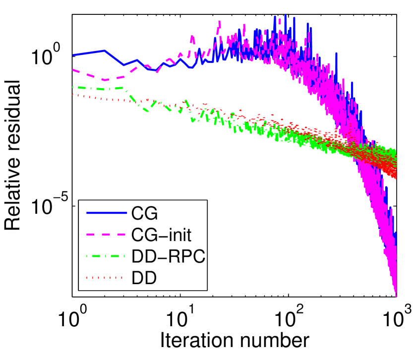
a) sarcos

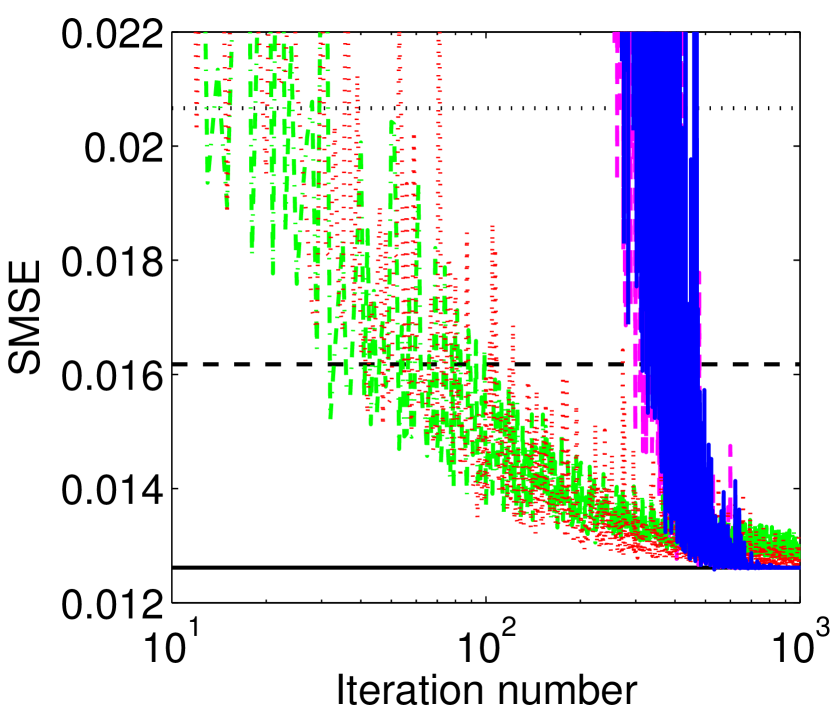
b) sarcos

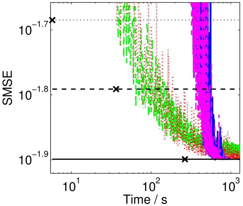
c) sarcos

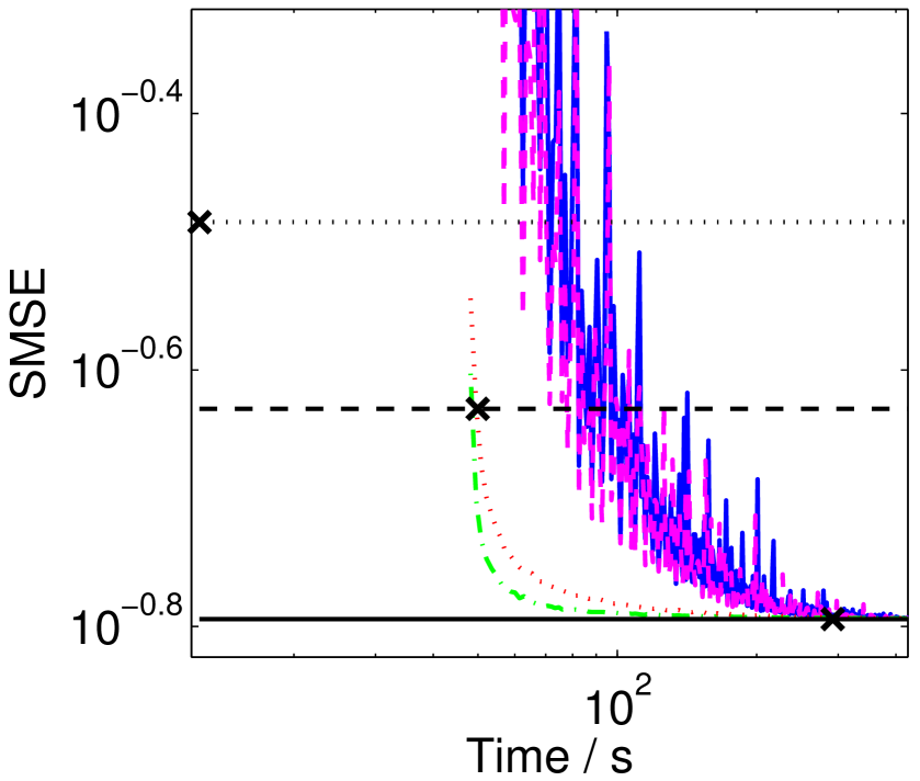
d) synth8

Figure 1: Experiments with 16,384 training points. CG: conjugate gradients; DD: ‘domain decomposition’ with 16 randomly chosen clusters; CG-init: CG initialized with one iteration of DD (CG’s starting point of zero isn’t responsible for bad early behaviour); DD-RPC: clusters were chosen with recursive projection clustering (Section 1.3). The horizontal lines give test performance for SoD with 4,096, 8,192 and 16,384 training points. Crosses on these lines also show the time taken.

Figure 1a) plots the ‘relative residual’, $\|(K\!+\!\sigma^{2}I)\mbox{\boldmath{$\alpha$}}_{t}-\mathbf{y}\|/\|\mathbf{y}\|$, the convergence diagnostic used by Li et al. (2007, Fig. 2), against iteration number for both their method and CG, where $\mbox{\boldmath{$\alpha$}}_{t}$ is the approximation to $\alpha$ obtained at iteration $t$. We reproduce the result that CG gives higher and fluctuating residuals for early iterations. However, by running the simulation for longer, and plotting on a log scale, we see that CG converges, according to this measure, much faster at later iterations. Figure 1a) is not directly useful for choosing between the methods however, because we do not know how many iterations are required for a competitive test-error.

Figure 1b) instead plots test-set SMSE, and adds reference lines for the SMSEs obtained by subsets with 4,096, 8,192 and 16,384 training points. We now see that 50 iterations are insufficient for meaningful convergence on this problem. Figure 1c) plots the SMSE against computer time taken on our machine. SoD performs better than the iterative methods.

These results depend on the dataset and hyperparameters. Figure 1d) shows the test-set SMSE progression against time for 16,384 points from synth8 using the true hyperparameters. Here CG takes a similar time to direct Cholesky solving. However, there is now a part of the error-time plot where the DD approach has better SMSEs at smaller times than either CG or SoD.

The timing results are heavily implementation and architecture dependent. For example, the results reported so far were run on a single 3 GHz core. On our machines, the iterative methods scale less well when deployed on multiple CPU cores. Increasing the number of cores to four (using Matlab, which uses Intel’s MKL), the time to perform a $16384\!\times\!16384$ Cholesky decomposition decreased by a factor of 3.1, whereas a matrix vector multiply improved by only a factor of 1.7.

3.2 Results for IFGT

We focus here on whether the IFGT provides fast MVMs for the datasets in our comparison. We used the isotropic squared-exponential kernel (which has one lengthscale parameter shared over all dimensions). For each of the four datasets we randomly chose 5000 datapoints to construct a kernel matrix, and a 5000-element random vector (with elements sampled from $U[0,1]$). Figure 2 shows the MVM time as a function of lengthscale. For synth2 and synth8 the known lengthscale is 1. For the two other problems, and indeed many standardized regression problems, lengthscales of  $\approx\!1$ (the width of the input distribution) are also appropriate. Figure 2 shows that useful MVM speedups over a direct implementation are only obtained for synth2. The result on sarcos is consistent with Raykar and Duraiswami (2007)’s result that IFGT does not accelerate GPR on this dataset.

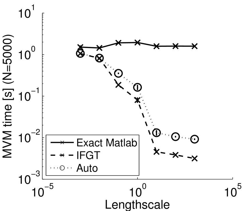
synth2

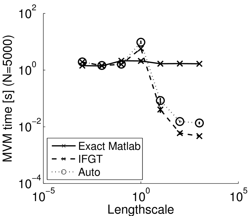
synth8

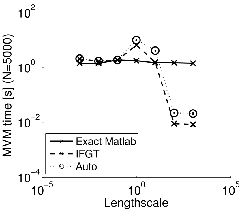
chem

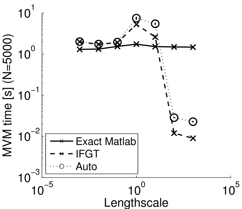
sarcos

Figure 2: Plot of time vs lengthscale using IFGT for matrix-vector multiplication (MVM) on the four datasets. The Auto method was introduced in (Raykar and Duraiswami, 2007) as a way to speed up IFGT in some regimes.

3.3 Comparison of SoD, FITC, Hybrid and Local GPR

All of the experiments below used the squared exponential kernel with ARD parameterization (Rasmussen and Williams, 2006, p106). The test times given below include computation of the predictive variances.

SoD was run with $m$ ascending in powers of 2 from $32,64\ldots$ up to $4096$. FITC was run with $m$ ranging from $8$ to $512$ in powers of two; this is smaller than for SoD as FITC is much more memory intensive. Local was run with $m$ ranging from $16$ to $2048$ in powers of two. For all experiments the selection of the subset/inducing points/clusters has a random aspect, and we performed five runs.

In Figure 3 we plot the test set SMSE against hyperparameter training time (left column), and test time (right column) for the four methods on the four datasets. Figure 4 shows similar plots for the test set MSLL. When there are further choices to be made (e.g. subset selection methods, joint/separate estimation of hyperparameters), we generally present the best results obtained by the method; these choices are detailed at the end of this section for each dataset individually. Further details including tables of learned hyperparameters can be found in Chalupka (2011), although the experiments were re-run for this paper, so there are some differences between the two.

The empirical times deviate from theory (Table 1) most for the Local method for small $m$. There is overhead due to the creation of many small matrices in Matlab, so that (for example) $m=32$ is always slower (on our four datasets) than $m=64$ and $m=128$. This effect is demonstrated explicitly in (Chalupka, 2011, Fig. 4.1), and accounts for the bending back observed in the plots for Local. (This is present on all four datasets, but can be difficult to see in some of the plots.)

Looking at the hyperparameter training plots (left column), it is noticeable that SoD and FITC reduce monotonically with increasing time, and that SoD outperforms FITC on all datasets (i.e. for the same amount of time, the SoD performance is better). On the test time plots (right column) the pattern between SoD and FITC is reversed, with FITC being superior. These results are consistent with theoretical scalings (Table 1): at training time FITC has worse scaling, at test time its scaling is the same, and it turns out that its more sophisticated approximation does give better results.

Comparing Hybrid to SoD for hyperparameter learning, we note a general improvement in performance for very similar time; this is because the additional cost of one FITC training step at the end is small relative to the time taken to optimize the hyperparameters using the SoD approximation of the marginal likelihood. At test time the Hybrid results are inferior to FITC for the same $m$ as expected, but the faster hyperparameter learning time means that larger subset sizes can be used with Hybrid.

For Local, the most noticeable pattern is that the run time does not change monotonically with $m$. We also note that for small $m$ the other methods can make faster approximations than Local can for any value of $m$. For Local there is a general trend for larger $m$ to produce better results, although on sarcos the error actually increases with $m$, and for synth2 the SMSE error rises for $m=1024,\;2048$. However, Local often gives better performance than the other methods in the time regimes where it operates.

We now comment on the specific datasets:

synth2: This function was fairly easy to learn and all methods were able to obtain good performance (with SMSE close to the noise level of $10^{-6}$) for sufficiently large $m$. For SoD and FITC, it turned out that FPC gave significantly better results than random subset selection. FPC distributes the inducing points in a more regular fashion in the space, instead of having multiple close by in regions of high density. For Local, the joint estimation of hyperparameters was found to be significantly better than separate; this result makes sense as the target function is actually drawn from a single GP. For FITC and Hybrid the plots are cut off at $m=128$ and $m=256$ respectively, as numerical instabilities in the gpml FITC code for larger $m$ values gave larger errors.

synth8: This function was difficult for all methods to learn, notice the slow decrease in error as a function of time. The SMSE obtained is far above the noise level of $10^{-3}$. Both SoD and FITC did slightly better when selecting the inducing points randomly. For the Local method, again joint estimation of hyperparameters was found to be superior, as for synth2. For both synth2 and synth8 we note that the lengthscales learned by the FITC approximation did not converge to the true values even for the largest $m$, while convergence was observed for SoD and Local; see Appendix 1 in Chalupka (2011) for full details.

chem: Both SoD and FITC did slightly better when selecting the inducing points randomly. Local with joint and separate hyperparameter training gave similar results. We report results on the joint method, for consistency with the other datasets.

sarcos: For SoD and FITC, FPC gave very slightly better results than random. Local with joint hyperparameter training did better than separate training.

synth2
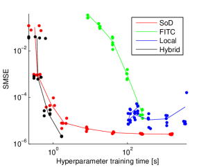
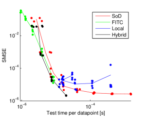
synth8
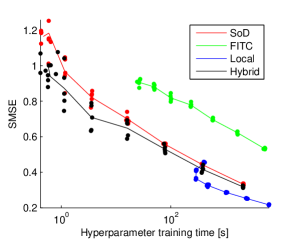
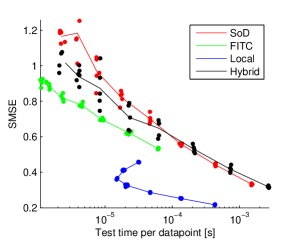
chem
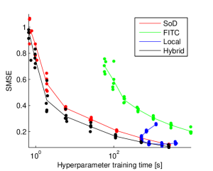
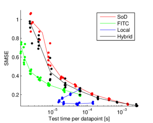
sarcos

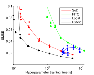
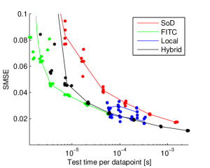
Figure 3: SMSE (log scale) as a function of time (log scale) for the four datasets. Left: hyperparameter training time. Right: test time per test point (including variance computations, despite not being needed to report SMSE). Points give the result for each run; lines connect the means of the 5 runs at each $m$.

synth2
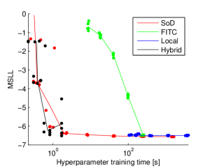
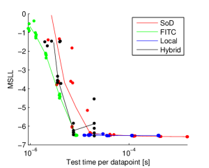
synth8
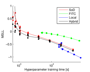
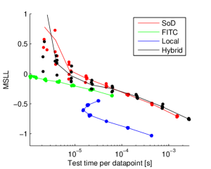
chem
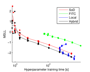
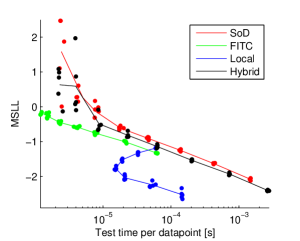
sarcos

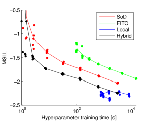
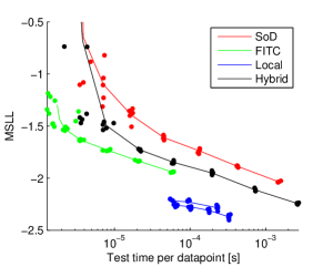
Figure 4: MSLL as a function of time (log scale) for the four datasets. Left: hyperparameter training time. Right: test time per test point. Points give the result for each run; lines connect the means of the 5 runs at each $m$.

3.4 Comparison with Prediction using the Generative Hyperparameters

For the synth2 and synth8 datasets it is possible to compare the results with learned hyperparameters against those obtained with hyperparameters fixed to the true generative values. We refer to these as the learned and fixed hyperparameter settings.

For the SoD and Local methods there is good agreement between the learned and fixed settings, although for SoD the learned setting generally performs worse on both SMSE and MSLL for small $m$, as would be expected given the small data sizes. The learned and fixed settings are noticeably different for SoD for $m\leq 128$ on synth2, and $m\leq 512$ on synth8.

For FITC there is also good agreement between the learned and fixed settings, although on synth8 we observed that the learned model slightly outperformed the fixed model by around 0.05 nats for MSLL, and by up to 0.05 for SMSE. This may suggest that for FITC the hyperparameters that produce optimal performance may not be the generative ones.

4 Future directions

We have seen that Local GPR can sometimes make better predictions than the other methods for some ranges of available computer time. However, our implementation suffers from unusual scaling behaviour at small $m$ due to the book-keeping overhead required to keep track of thousands of small matrices. More careful, lower-level programming than our Matlab code might reduce these problems.

It is possible to combine the SoD with other methods. As a dataset’s size tends to infinity, SoD (with random selection) will always beat the other approximations that we have considered, as SoD is the only method with no $n$-dependence (Table 1). Of course the other approximate methods, such as FITC, could also be run on a subset. Investigating how to simultaneously choose the dataset size to consider, $n$, and the control parameter of an approximation, $m$, has received no attention in the literature to our knowledge.

Some methods will have more choices than a single control parameter $m$. For example, Snelson and Ghahramani (2006) optimized the locations of the $m$ inducing points, potentially improving test-time performance at the expense of a longer training time. A potential future area of research is working out how to intelligently balance the computer time spent on selecting and moving inducing points, while performing hyperparameter training, and choosing a subset size. Developing methods that work well in a wide variety of contexts without tweaking might be challenging, but success could be measured using the framework of this paper.

5 Conclusions

We have advocated the comparison of GPR approximation methods on the basis of prediction quality obtained vs compute time. We have explored the times required for the hyperparameter learning, training and testing phases, and also addressed other factors that are relevant for comparing approximations. We believe that future evaluations of GP approximations should consider these factors (Sec. 2), and compare error-time curves with standard approximations such as SoD and FITC. To this end we have made our data and code available to facilitate comparisons. Most papers that have proposed GP approximations have not compared to SoD, and on trying the methods it is often difficult to get appreciably below SoD’s error-time curve for the learning phase. Yet these methods are often more difficult to run and more limited in applicability than SoD.

On the datasets we considered, SoD and Hybrid dominate FITC in terms of hyperparameter learning. However, FITC (for as long as we ran it) gave better accuracy for a given test time. SoD, Hybrid and FITC behaved monotonically with subset/inducing-set size $m$, making $m$ a useful control parameter. The Local method produces more varied results, but can provide a win for some problems and cluster sizes. Comparison of the iterative methods, CG and DD, to SoD revealed that they shouldn’t be run for a small fixed number of iterations, and that performance can be comparable with simpler, more stable approaches. Faster MVM methods might make iterative methods more compelling, although the IFGT method only provided a speedup on the synth2 problem out of our datasets. Assuming that hyperparameter learning is the dominant factor in computation time, the results presented above point to the very simple Subset of Data method (or the Hybrid variant) as being the leading contender. We hope this will act as a rallying cry to those working on GP approximations to beat this “dumb” method. This can be addressed both by empirical evaluations (as presented here), and by theoretical work.

Many approximate methods require choosing subsets of partitions of the data. Although farthest point clustering (FPC) improved SoD and FITC on the low-dimensional (easiest) problem, simple random subset selection worked similarly or better on all other datasets. Random selection also has better scaling (no $n$-dependence) for the largest-scale problems. The choice of partitioning scheme was important for Local regression: Our preliminary experiments showed that performance was severely hampered by many small clusters produced by FPC; we recommend our recursive partitioning scheme (RPC).

Acknowledgments

We thank the anonymous referees whose comments helped improve the paper. We also thank Carl Rasmussen, Ed Snelson and Joaquin Quiñinero-Candela for many discussions on the comparison of GP approximation methods.

This work is supported in part by the IST Programme of the European Community, under the PASCAL2 Network of Excellence, IST-2007-216886. This publication only reflects the authors’ views.

References

- Adams et al. (2010) Ryan P. Adams, George E. Dahl, and Iain Murray. Incorporating side information into probabilistic matrix factorization using Gaussian processes. In Proceedings of the 26th Conference on Uncertainty in Artificial Intelligence, pages 1–9. AUAI Press, 2010.
- Blum et al. (1973) Manuel Blum, Robert W. Floyd, Vaughan Pratt, Ronald L. Rivest, and Robert E. Tarjan. Time bounds for selection. Journal of Computer and System Sciences, 7:448–461, 1973.
- Chalupka (2011) Krzysztof Chalupka. Empirical evaluation of Gaussian process approximation algorithms. Master’s thesis, School of Informatics, University of Edinburgh, 2011. http://homepages.inf.ed.ac.uk/ckiw/postscript/Chalupka2011diss.pdf.
- Feder and Greene (1988) Tomás Feder and Daniel H. Greene. Optimal algorithms for approximate clustering. In Proceedings of the 20th ACM Symposium on Theory of Computing, pages 434–444. ACM Press, New York, USA, 1988. ISBN 0-89791-264-0. doi: http://doi.acm.org/10.1145/62212.62255.
- Freitas et al. (2006) Nando De Freitas, Yang Wang, Maryam Mahdaviani, and Dustin Lang. Fast Krylov methods for N-body learning. In Y. Weiss, B. Schölkopf, and J. Platt, editors, Advances in Neural Information Processing Systems 18, pages 251–258. MIT Press, 2006.
- Fritz et al. (2009) J. Fritz, I. Neuweiler, and W. Nowak. Application of FFT-based algorithms for large-scale universal Kriging problems. Math. Geosci., 41:509–533, 2009.
- Gibbs (1997) Mark Gibbs. Bayesian Gaussian processes for classification and regression. PhD thesis, University of Cambridge, 1997.
- Golub and Van Loan (1996) Gene H. Golub and Charles F. Van Loan. Matrix computations, third edition. The John Hopkins University Press, 1996.
- Gonzales (1985) Teofilo F. Gonzales. Clustering to minimize the maximum intercluster distance. Theoretical Computer Science, 38(2-3):293–306, 1985.
- Gray (2004) Alexander Gray. Fast kernel matrix-vector multiplication with application to Gaussian process learning. Technical Report CMU-CS-04-110, School of Computer Science, Carnegie Mellon University, 2004.
- Keerthi and Chu (2006) Sathiya Keerthi and Wei Chu. A matching pursuit approach to sparse Gaussian process regression. In Y. Weiss, B. Schölkopf, and J. Platt, editors, Advances in Neural Information Processing Systems 18, pages 643–650. MIT Press, Cambridge, MA, 2006.
- Lawrence et al. (2003) Neil Lawrence, Matthias Seeger, and Ralf Herbrich. Fast sparse Gaussian process methods: The informative vector machine. In S. Becker, S. Thrun, and K. Obermayer, editors, Advances in Neural Information Processing Systems 15, pages 625–632. MIT Press, 2003.
- Lawrence (2004) Neil D. Lawrence. Gaussian process latent variable models for visualization of high dimensional data. In Sebastian Thrun, Lawrence Saul, and Bernhard Schölkopf, editors, Advances in Neural Information Processing Systems 16, pages 329–336. MIT Press, 2004.
- Lázaro-Gredilla et al. (2010) Miguel Lázaro-Gredilla, Joaquin Quiñonero-Candela, Carl Edward Rasmussen, and Aníbal R. Figueiras-Vidal. Sparse spectrum Gaussian process regression. Journal of Machine Learning Research, 11:1865−1881, 2010.
- Li et al. (2007) Wenye Li, Kin-Hong Lee, and Kwong-Sak Leung. Large-scale RLSC learning without agony. In Proceedings of the 24th International Conference on Machine learning, pages 529–536. ACM Press New York, NY, USA, 2007.
- Liberty et al. (2007) Edo Liberty, Franco Woolfe, Per-Gunnar Martinsson, Vladimir Rokhlin, and Mark Tygert. Randomized algorithms for the low-rank approximation of matrices. Proceedings of the National Academy of Sciences, 104(51):20167–72, 2007.
- Malshe et al. (2007) M. Malshe, L. M. Raff, M. G. Rockey, M. Hagan, Paras M. Agrawal, and R. Komanduri. Theoretical investigation of the dissociation dynamics of vibrationally excited vinyl bromide on an ab initio potential-energy surface obtained using modified novelty sampling and feedforward neural networks. II. Numerical application of the method. J. Chem. Phys., 127(13):134105, 2007.
- Manzhos and Carrington (2008) Sergei Manzhos and Tucker Carrington, Jr. Using neural networks, optimized coordinates, and high-dimensional model representations to obtain a vinyl bromide potential surface. The Journal of Chemical Physics, 129:224104, 2008.
- Morariu et al. (2009) Vlad I Morariu, Balaji Vasan Srinivasan, Vikas C Raykar, Ramani Duraiswami, and Larry S Davis. Automatic online tuning for fast Gaussian summation. In D. Koller, D. Schuurmans, Y. Bengio, and L. Bottou, editors, Advances in Neural Information Processing Systems 21, pages 1113–1120, 2009.
- Murray (2009) Iain Murray. Gaussian processes and fast matrix-vector multiplies, 2009. Presented at the Numerical Mathematics in Machine Learning workshop at the 26th International Conference on Machine Learning (ICML 2009), Montreal, Canada. URL http://www.cs.toronto.edu/~murray/pub/09gp_eval/ (as of March 2011).
- Neal (1996) Radford M. Neal. Bayesian Learning for Neural Networks. Springer, New York, 1996. Lecture Notes in Statistics 118.
- Paciorek (2007) Christopher J. Paciorek. Bayesian smoothing with Gaussian processes using Fourier basis functions in the spectralGP package. Journal of Statistical Software, 19(2):1–38, 2007. URL http://www.jstatsoft.org/v19/i02.
- Quiñonero-Candela and Rasmussen (2005) Joaquin Quiñonero-Candela and Carl E. Rasmussen. A unifying view of sparse approximate Gaussian process regression. Journal of Machine Learning Research, 6:1939–1959, 2005.
- Quiñonero-Candela et al. (2007) Joaquin Quiñonero-Candela, Carl E. Rasmussen, and Christopher K. I. Williams. Approximation methods for Gaussian process regression. In Léon Bottou, Olivier Chapelle, Dennis DeCoste, and Jason Weston, editors, Large Scale Learning Machines, pages 203–223. MIT Press, 2007.
- Rasmussen and Williams (2006) Carl E. Rasmussen and Christopher K. I. Williams. Gaussian Processes for Machine Learning. MIT Press, Cambridge, Massachusetts, 2006.
- Raykar and Duraiswami (2007) Vikas C. Raykar and Ramani Duraiswami. Fast large scale Gaussian process regression using approximate matrix-vector products. In Learning workshop 2007, San Juan, Peurto Rico, 2007. Available from: http://www.umiacs.umd.edu/~vikas/publications/raykar_learning_workshop_%2007_full_paper.pdf.
- Shen et al. (2006) Yirong Shen, Andrew Ng, and Matthias Seeger. Fast Gaussian process regression using KD-trees. In Y. Weiss, B. Schölkopf, and J. Platt, editors, Advances in Neural Information Processing Systems 18, pages 1225–1232. MIT Press, 2006.
- Snelson and Ghahramani (2006) E. Snelson and Z. Ghahramani. Sparse Gaussian processes using pseudo-inputs. In Y. Weiss, B. Schölkopf, and J. Platt, editors, Advances in Neural Information Processing Systems 18, pages 1257–1264, 2006.
- Snelson (2007) Edward Snelson. Flexible and efficient Gaussian process models for machine learning. PhD thesis, Gatsby Computational Neuroscience Unit, University College London, 2007.
- Snelson and Ghahramani (2007) Edward Snelson and Zoubin Ghahramani. Local and global sparse Gaussian process approximations. In M. Meila and X. Shen, editors, Artificial Intelligence and Statistics 11. Omnipress, 2007.
- Sudderth and Jordan (2009) Erik Sudderth and Michael Jordan. Shared segmentation of natural scenes using dependent Pitman-Yor processes. In D. Koller, D. Schuurmans, Y. Bengio, and L. Bottou, editors, Advances in Neural Information Processing Systems 21, pages 1585–1592, 2009.
- Titsias (2009) Michalis Titsias. Variational learning of inducing variables in sparse Gaussian processes. In Artificial Intelligence and Statistics 12, volume 5, pages 567–574. JMLR: W&CP, 2009.
- Wikle et al. (2001) Christopher K Wikle, Ralph F Milliff, Doug Nychka, and L Mark Berliner. Spatiotemporal hierarchical Bayesian modeling: tropical ocean surface winds. Journal of the American Statistical Association, 96(454):382–397, 2001.
- Yang et al. (2005) Changjiang Yang, Ramani Duraiswami, and Larry Davis. Efficient kernel machines using the improved fast Gauss transform. In Lawrence K. Saul, Yair Weiss, and Léon Bottou, editors, Advances in Neural Information Processing Systems 17, pages 1561–1568. MIT Press, 2005.