Properties of finite Gaussians and
the discrete-continuous transition

Abstract

Weyl’s formulation of quantum mechanics opened the possibility of studying the dynamics of quantum systems both in infinite-dimensional and finite-dimensional systems. Based on Weyl’s approach, generalized by Schwinger, a self-consistent theoretical framework describing physical systems characterised by a finite-dimensional space of states has been created. The used mathematical formalism is further developed by adding finite-dimensional versions of some notions and results from the continuous case. Discrete versions of the continuous Gaussian functions have been defined by using the Jacobi theta functions. We continue the investigation of the properties of these finite Gaussians by following the analogy with the continuous case. We study the uncertainty relation of finite Gaussian states, the form of the associated Wigner quasi-distribution and the evolution under free-particle and quantum harmonic oscillator Hamiltonians. In all cases, a particular emphasis is put on the recovery of the known continuous-limit results when the dimension $d$ of the system increases.

1 Introduction

The continuous Gaussian functions

$$g_{\kappa}:\mathbb{R}\longrightarrow\mathbb{R},\qquad g_{\kappa}(x)=\mathrm{e}^{-\frac{\kappa}{2}x^{2}}\qquad\qquad\qquad\kappa\!\in\!(0,\infty)$$

play a fundamental role in physics, particularly in quantum mechanics, due to their remarkable properties, among which we mention:

1. With the Fourier transform defined as

   $$\mathcal{F}[f](\xi)=\frac{1}{\sqrt{2\pi}}\int_{-\infty}^{\infty}{\rm e}^{{\rm i}\xi x}f(x)\,dx$$

   we have

   $$\mathcal{F}[g_{\kappa}]=\frac{1}{\sqrt{\kappa}}\,g_{\frac{1}{\kappa}}.$$ (1)

2. The function $g_{1}$ is an eigenfunction of a second-order differential operator

   $$\left(-\frac{d^{2}}{dx^{2}}+x^{2}\right){\rm e}^{-\frac{1}{2}x^{2}}={\rm e}^{-\frac{1}{2}x^{2}}.$$ (2)

3. The function $g_{\kappa}$ is a minimum uncertainty state for the coordinate-momentum

   $$\Delta\hat{x}\,\Delta\hat{p}=\frac{1}{2}$$ (3)

4. The Wigner quasi-distribution [25] corresponding to $g_{\kappa}$ defined as

   $$W(x,p)=\frac{1}{\pi}\int_{-\infty}^{\infty}du\,\mathrm{e}^{2{\rm i}pu}g_{\kappa}\left(x-u\right)\,g_{\kappa}^{*}\left(x+u\right)$$

   is, up to a multiplicative constant, a product of two Gaussian functions

   $$W(x,p)=2\sqrt{\frac{\pi}{\kappa}}\,\mathrm{e}^{-\kappa x^{2}}\,\mathrm{e}^{-\frac{1}{\kappa}p^{2}}.$$ (4)

Figure 1: The functions $\mathfrak{g}_{1/3}$ (left), $\mathfrak{g}_{1}$ (center) and $\mathfrak{g}_{3}$ (right) in the case $d=31$.

Let $d=2s+1\in\{3,5,7,...\}$ be a fixed odd positive integer, and let $\mathbb{Z}_{d}\!=\!\mathbb{Z}/d\mathbb{Z}$ be the ring of integers modulo $d$ for which we use $\{-s,-s\!+\!1,...,s\!-\!1,s\}$ as a set of ‘standard’ representatives. The number $d$ represents the dimension of the Hilbert space describing the states of the investigated quantum systems.

The Jacobi theta function [11, 21, 24]

$$\theta_{3}(z,\tau)=\sum_{\alpha=-\infty}^{\infty}{\rm e}^{{\rm i}\pi\tau\alpha^{2}}\,{\rm e}^{2\pi{\rm i}\alpha z}$$

has several remarkable properties among which we mention:

$$\theta_{3}(z+m+n\tau,\tau)={\rm e}^{-{\rm i}\pi\tau n^{2}}\,{\rm e}^{-2\pi{\rm i}nz}\,\theta_{3}(z,\tau)$$

$$\theta_{3}(z,{\rm i}\tau)=\frac{1}{\sqrt{\tau}}\,{\rm exp}^{-\frac{\pi z^{2}}{\tau}}\,\theta_{3}\left(\frac{z}{{\rm i}\tau},\frac{\rm i}{\tau}\right)$$

and [19]

$$\theta_{3}\left(\frac{k}{d},\frac{{\rm i}\kappa}{d}\right)=\frac{1}{\sqrt{\kappa d}}\,\sum_{n=-s}^{s}{\rm e}^{-\frac{2\pi{\rm i}}{d}kn}\,\theta_{3}\left(\frac{n}{d},\frac{\rm i}{\kappa d}\right).$$ (5)

For any $\kappa\in(0,\infty)$ the function

$$\mathfrak{g}_{\kappa}:\mathbb{Z}_{d}\longrightarrow\mathbb{R},\qquad\mathfrak{g}_{\kappa}(n)=\sum_{\alpha=-\infty}^{\infty}\mathrm{e}^{-\frac{\kappa\pi}{d}(\alpha d+n)^{2}}$$

can be expressed in terms of the Jacobi function $\theta_{3}$ as

$$\mathfrak{g}_{\kappa}(n)=\frac{1}{\sqrt{\kappa d}}\,\theta_{3}\left(\frac{n}{d},\frac{{\rm i}}{\kappa d}\right)$$

and by using the finite Fourier transform

$$F[\psi](k)=\frac{1}{\sqrt{d}}\sum_{n=-s}^{s}{\rm e}^{\frac{2\pi{\rm i}}{d}kn}\psi(n)$$

Ruzzi’s relation (5) can be written in a form identical to (1), namely,

$$F[\mathfrak{g}_{\kappa}]=\frac{1}{\sqrt{\kappa}}\,\mathfrak{g}_{\frac{1}{\kappa}}.$$ (6)

This property of the function $\mathfrak{g}_{\kappa}$ and the shape of its graph (see figure 1) show that it can be regarded as a finite version of the Gaussian function $g_{\kappa}$. We call $\mathfrak{g}_{\kappa}$ a finite Gaussian, and our main purpose is to prove the existence of a finite version for the relations (1)-(4). We recover well-known results for continuous Gaussians for large $d$ values, i.e. at the discrete-continuous transition, and emphasize conditions under which the evolution of continuous Gaussian states can be retrieved from the evolution of their discrete counterparts.

The finite Gaussians $\mathfrak{g}_{\kappa}$ represent a generalization of Mehta’s function $f_{0}$, and the relation (6) is a generalization of Mehta’s relation $F[f_{0}]=f_{0}$. More precisely, Mehta has proved [15] that the functions

$$\begin{array}[]{l}f_{k}(n)=\sum\limits_{\alpha=-\infty}^{\infty}\mathrm{e}^{-\frac{\pi}{d}(\alpha d+n)^{2}}\,H_{k}\left(\sqrt{\frac{2\pi}{d}}(\alpha d+n)\right)\end{array}$$

defined by using the Hermite polynomials are eigenvectors of the finite Fourier transform

$$F[f_{k}]={\rm i}^{k}\,f_{k}\qquad{\rm for\ any}\quad k\!\in\!\{0,1,2,...\}.$$

Since $H_{0}(x)=1$, we have $f_{0}=\mathfrak{g}_{1}$ and the relation $F[f_{0}]=f_{0}$ coincides to $F[\mathfrak{g}_{1}]=\mathfrak{g}_{1}$. Mehta’s results are mainly based on the following remarks, which we will use in the following:

• A periodic function with period $d$, namely,

  $$\begin{array}[]{l}\Phi:\mathbb{Z}\longrightarrow\mathbb{R},\qquad\Phi(n)=\sum\limits_{\alpha=-\infty}^{\infty}\varphi\left(\sqrt{\frac{2\pi}{d}}(\alpha d+n)\right)\end{array}$$

  can be defined by starting from any function $\varphi:\mathbb{R}\longrightarrow\mathbb{R}$ for which the series is absolutely convergent. This is similar to a Zak [26] or Weil [23] transform.

• The relation

  $$\sum_{\alpha=-\infty}^{\infty}\int_{\alpha\sqrt{2\pi d}}^{(\alpha+1)\sqrt{2\pi d}}\varphi(x)\,dx=\int_{-\infty}^{\infty}\varphi(x)\,dx$$

  is true for any function $\varphi:\mathbb{R}\longrightarrow\mathbb{R}$ for which the integral is convergent.

• The relation

  $$\sum_{\alpha=-\infty}^{\infty}\varphi(\alpha)=\sum_{n=-s}^{s}\sum_{\alpha=-\infty}^{\infty}\varphi(\alpha d+n)$$

  is satisfied for any function $\varphi:\mathbb{Z}\longrightarrow\mathbb{R}$ for which the series is absolutely convergent.

In section 2 we review some elements of the mathematical formalism used in the case of the quantum systems with finite-dimensional Hilbert space, in a form suitable for our purpose. We show that in the case of the free evolution, the time dependent state is periodic in time. The behaviour of the commutator of the position and momentum operators in the limit of large $d$ is investigated in section 3. Ruzzi has obtained the relation (6) by using the properties of $\theta$-functions. In section 4 we present an elementary proof based on a)-c) for this finite version of relation (1), and show that $\mathfrak{g}_{1}$ is almost a minimum uncertainty state. In section 5 we investigate numerically the quantum oscillator Hamiltonian. The tendency to have equidistant energy levels becomes evident only for $d$ large enough. In section 6 we show, for the first time to our knowledge, that the existence of commensurate or equidistant energy levels is a sufficient condition for the occurrence of revivals.

In section 7, by using a)-c) as mathematical tools, we prove that the Wigner function corresponding to a finite Gaussian can be written as a sum of four products of finite Gaussians. The obtained formula is our main result, and can be regarded as a finite version of the relation (4). In the particular case $\kappa=1$, an expression of the Wigner function corresponding to a finite Gaussian $\mathfrak{g}_{1}$ has been previously obtained by Marchiolli and Ruzzi [12]. They proved that, up to a multiplicative constant, the Wigner function corresponding to

$$\mathfrak{g}_{1}(n)=\frac{1}{\sqrt{d}}\,\theta_{3}\left(\frac{n}{d},\frac{{\rm i}}{d}\right)$$

is

$$W(n,m)=\theta_{3}\left(\frac{n}{d},\frac{{\rm i}}{2d}\right)\,\theta_{3}\left(\frac{2m}{d},\frac{2{\rm i}}{d}\right)+\theta_{4}\left(\frac{n}{d},\frac{{\rm i}}{2d}\right)\,\theta_{2}\left(\frac{2m}{d},\frac{2{\rm i}}{d}\right)$$

where $\theta_{2}$ and $\theta_{4}$ are the Jacobi functions

$$\theta_{2}(z,\tau)=\sum_{\alpha=-\infty}^{\infty}{\rm e}^{{\rm i}\pi\tau\left(\alpha+\frac{1}{2}\right)^{2}}\,{\rm e}^{2\pi{\rm i}\left(\alpha+\frac{1}{2}\right)z}$$

and

$$\theta_{4}(z,\tau)=\sum_{\alpha=-\infty}^{\infty}(-1)^{\alpha}{\rm e}^{{\rm i}\pi\tau\alpha^{2}}\,{\rm e}^{2\pi{\rm i}\alpha z}.$$

2 Quantum systems with finite-dimensional Hilbert space

In the case of a quantum particle moving along a straight line, the possible positions form the set $\mathbb{R}=(-\infty,\infty)$, and the space describing the states of the system is the infinite-dimensional Hilbert space $L^{2}(\mathbb{R})$ of all the square integrable functions $\psi:\mathbb{R}\longrightarrow\mathbb{C}$.

We obtain a very simplified version of this continuous one-dimensional system by assuming that we can distinguish only a finite number $d$ of positions for our particle. In this simplified version, the space describing the states of the system is the $d$-dimensional Hilbert space $\mathbb{C}^{d}$. Assuming that $d$ is an odd number, $d\!=\!2s\!+\!1$, the space $\mathbb{C}^{d}$ can be identified with the space $\mathcal{H}$ of all the functions

$$\psi:\{-s,-s\!+\!1,...,s\!-\!1,s\}\longrightarrow\mathbb{C}$$

by using the one-to-one mapping

$$\mathcal{H}\longrightarrow\mathbb{C}^{d}:\psi\mapsto(\psi(-s),\psi(-s+1),...,\psi(s-1),\psi(s)).$$

We choose an orthonormal basis $\{|n\rangle\}_{n\in\mathbb{Z}_{d}}$ in $\mathcal{H}$ and define the ‘position’ operator

$$\begin{array}[]{l}Q:\mathcal{H}\longrightarrow\mathcal{H},\qquad Q=\sqrt{\frac{2\pi}{d}}\sum\limits_{n=-s}^{s}n\,|n\rangle\langle n|.\end{array}$$ (7)

The finite Fourier transform

$$F:\mathcal{H}\longrightarrow\mathcal{H},\qquad F=\frac{1}{\sqrt{d}}\sum_{n,n^{\prime}=-s}^{s}{\rm e}^{\frac{2\pi{\rm i}}{d}nn^{\prime}}|n\rangle\langle n^{\prime}|$$ (8)

allows us to consider a second orthonormal basis $\{|\tilde{k}\rangle\}_{k\in\mathbb{Z}_{d}}$, where

$$|\tilde{k}\rangle\!=\!F|k\rangle=F^{+}|-k\rangle\!=\!\frac{1}{\sqrt{d}}\sum_{n=-s}^{s}{\rm e}^{\frac{2\pi{\rm i}}{d}kn}|n\rangle$$

and to define the ‘momentum’ operator

$$\begin{array}[]{l}P:\mathcal{H}\longrightarrow\mathcal{H},\qquad P=\sqrt{\frac{2\pi}{d}}\sum\limits_{k=-s}^{s}k\,|\tilde{k}\rangle\langle\tilde{k}|.\end{array}$$

The operators $Q$ and $P$ have the same spectrum, namely,

$$\mathcal{S}_{d}=\left\{-s\sqrt{\frac{2\pi}{d}},\ (-s\!+\!1)\sqrt{\frac{2\pi}{d}},\ ...\ ,\ (s\!-\!1)\sqrt{\frac{2\pi}{d}},\ s\sqrt{\frac{2\pi}{d}}\right\}.$$

Since

$$\lim_{d\rightarrow\infty}\sqrt{\frac{2\pi}{d}}=0\qquad{\rm and}\qquad\lim_{d\rightarrow\infty}(\pm s)\sqrt{\frac{2\pi}{d}}=\pm\infty$$

in the limit $d\rightarrow\infty$, the spectra of $Q$ and $P$ correspond in a certain sense to $(-\infty,\infty)$.

Each state $|\psi\rangle\!\in\!\mathcal{H}$ can be expanded as

$$|\psi\rangle\!=\!\sum_{n=-s}^{s}\psi(n)\,|n\rangle\!=\!\sum_{k=-s}^{s}\tilde{\psi}(k)\,|\tilde{k}\rangle$$

where the functions  $\psi\!:\!\mathbb{Z}_{d}\!\longrightarrow\!\mathbb{C}\!:n\mapsto\psi(n)$  and  $\tilde{\psi}\!:\!\mathbb{Z}_{d}\!\longrightarrow\!\mathbb{C}\!:k\mapsto\tilde{\psi}(k)$  satisfying

$$\psi(n)\!=\!\langle n|\psi\rangle\!=\!\frac{1}{\sqrt{d}}\sum_{k=-s}^{s}{\rm e}^{\frac{2\pi{\rm i}}{d}kn}\tilde{\psi}(k)\,,\qquad\tilde{\psi}(k)\!=\!\langle\tilde{k}|\psi\rangle\!=\!\frac{1}{\sqrt{d}}\sum_{n=-s}^{s}{\rm e}^{-\frac{2\pi{\rm i}}{d}kn}\psi(n)\,.$$ (9)

are the corresponding ‘wavefunctions’ in the position and momentum representations [5]. The operators $Q$ and $P$ satisfy the relations

$$FQF^{+}\!=\!P\qquad\qquad FPF^{+}\!=\!-Q.$$

The displacement operators $A\,,B\!:\!\mathcal{H}\!\longrightarrow\!\mathcal{H}$

$$A\!=\!{\rm e}^{-{\rm i}\sqrt{2\pi/d}\,P}\!=\!\!\sum_{k=-s}^{s}{\rm e}^{-\frac{2\pi{\rm i}}{d}k}|\tilde{k}\rangle\langle\tilde{k}|\,,\qquad B\!=\!{\rm e}^{{\rm i}\sqrt{2\pi/d}\,Q}\!=\!\sum_{\ell=-s}^{s}{\rm e}^{\frac{2\pi{\rm i}}{d}\ell}|\ell\rangle\langle\ell|\,,$$ (10)

are single-valued and satisfy the relations

$$\begin{array}[]{lll}A|\ell\rangle=|\ell\!+\!1\rangle\,,&A|\tilde{k}\rangle\!=\!{\rm e}^{-\frac{2\pi{\rm i}}{d}k}|\tilde{k}\rangle\,,&A^{d}=B^{d}=\mathbb{I}\,,\\[5.69054pt] B|\ell\rangle\!=\!{\rm e}^{\frac{2\pi{\rm i}}{d}\ell}|\ell\rangle\,,&B|\tilde{k}\rangle=|\widetilde{k\!+\!1}\rangle\,,&A^{\alpha}B^{\beta}\!=\!{\rm e}^{-\frac{2\pi{\rm i}}{d}\alpha\beta}B^{\beta}A^{\alpha}\,.\end{array}$$

The general displacements operators [22, 20]

$$D(\alpha,\beta)={\rm e}^{\frac{\pi{\rm i}}{d}\alpha\beta}\,A^{\alpha}B^{\beta}\qquad{\rm where}\quad(\alpha,\beta)\in\mathbb{Z}_{d}\times\mathbb{Z}_{d}$$ (11)

define a projective representation of the finite Weyl group. The vectors $\{|\alpha,\beta\rangle\}_{\alpha,\beta=-s}^{s}$, where

$$|\alpha,\beta\rangle=D(\alpha,\beta)\,\frac{\mathfrak{g}_{1}}{||\mathfrak{g}_{1}||}=\frac{{\rm e}^{-\frac{\pi{\rm i}}{d}\alpha\beta}}{||\mathfrak{g}_{1}||}\sum_{j=-s}^{s}{\rm e}^{\frac{2\pi{\rm i}}{d}\beta j}\,\,\mathfrak{g}_{1}(j\!-\!\alpha)\,|j\rangle$$

satisfy the resolution of identity[5, 27]

$$\frac{1}{d}\sum_{\alpha,\beta=-s}^{s}|\alpha,\beta\rangle\langle\alpha,\beta|=\mathbb{I}.$$

The tight frame $\{|\alpha,\beta\rangle\}_{\alpha,\beta=-s}^{s}$ can be regarded as a finite system of coherent states [7] labeled by using the set ${Z}_{d}\!\times\!\mathbb{Z}_{d}$, directly related to the finite phase space $\mathcal{S}_{d}\!\times\!\mathcal{S}_{d}$.

The mathematical objects defined above correspond in the large $d$ limit to those usually considered in the case of the quantum harmonic oscillator. An extensive list concerning this correspondence can be found in Table 1.

Table 1: Correspondence between continuous and $(2s\!+\!1)$-dimensional case.

• ${Continuous\ case}$	$(2s\!+\!1)-{dimensional\ case}$
  $(-\infty,\infty)$	$\mathcal{S}_{d}$
  $x$	$n\sqrt{\frac{2\pi}{d}}$
  $p$	$k\sqrt{\frac{2\pi}{d}}$
  $\langle x|x^{\prime}\rangle=\delta(x-x^{\prime})$	$\langle n|n^{\prime}\rangle=\delta_{nn^{\prime}}$
  $|\psi\rangle=\int dx\,\psi(x)\,|x\rangle$	$|\psi\rangle=\sum_{n=-s}^{s}\psi(n)\,|n\rangle$
  $\psi(x)=\langle x|\psi\rangle$	$\psi(n)=\langle n|\psi\rangle$
  $\hat{x}=\int dx\,x\,|x\rangle\langle x|$	$Q=\sqrt{\frac{2\pi}{d}}\sum\limits_{n=-s}^{s}n\,|n\rangle\langle n|$
  $\hat{x}\,|x\rangle=x\,|x\rangle$	$Q\,|n\rangle=n\sqrt{\frac{2\pi}{d}}\,|n\rangle$
  $\mathcal{F}=\frac{1}{\sqrt{2\pi}}\int\!\!\int dx^{\prime}\,dx\,{\rm e}^{{\rm i}x^{\prime}x}|x^{\prime}\rangle\langle x|$	$F=\frac{1}{\sqrt{d}}\sum_{n^{\prime},n=-s}^{s}{\rm e}^{\frac{2\pi{\rm i}}{d}n^{\prime}n}|n^{\prime}\rangle\langle n|$
  $\mathcal{F}|\psi\rangle=\frac{1}{\sqrt{2\pi}}\int\!\!\int dx^{\prime}\,dx\,{\rm e}^{{\rm i}x^{\prime}x}\psi(x)\,|x^{\prime}\rangle$	$F|\psi\rangle=\frac{1}{\sqrt{d}}\sum_{n^{\prime},n=-s}^{s}{\rm e}^{\frac{2\pi{\rm i}}{d}n^{\prime}n}\psi(n)\,|n^{\prime}\rangle$
  $\mathcal{F}|\psi\rangle=\int dx^{\prime}\,\mathcal{F}[\psi](x^{\prime})\,|x^{\prime}\rangle$	$\mathcal{F}|\psi\rangle=\sum_{n^{\prime}=-s}^{s}\mathcal{F}[\psi](n^{\prime})\,|n^{\prime}\rangle$
  $\mathcal{F}[\psi](x^{\prime})=\frac{1}{\sqrt{2\pi}}\int dx\,{\rm e}^{{\rm i}x^{\prime}x}\psi(x)$	$F[\psi](n^{\prime})=\frac{1}{\sqrt{d}}\sum_{n=-s}^{s}{\rm e}^{\frac{2\pi{\rm i}}{d}n^{\prime}n}\psi(n)$
  $|\tilde{p}\rangle=\mathcal{F}|p\rangle=\frac{1}{\sqrt{2\pi}}\int dx\,{\rm e}^{{\rm i}px}|x\rangle$	$|\tilde{k}\rangle=\mathcal{F}|k\rangle=\frac{1}{\sqrt{d}}\sum_{n=-s}^{s}{\rm e}^{\frac{2\pi{\rm i}}{d}kn}|n\rangle$
  $\langle x|\tilde{p}\rangle=\frac{1}{\sqrt{2\pi}}{\rm e}^{{\rm i}px}$	$\langle n|\tilde{k}\rangle=\frac{1}{\sqrt{d}}{\rm e}^{\frac{2\pi{\rm i}}{d}kn}$
  $\langle\tilde{p}|\tilde{p}^{\prime}\rangle=\delta(p-p^{\prime})$	$\langle\tilde{k}|\tilde{k}^{\prime}\rangle=\delta_{kk^{\prime}}$
  $|\psi\rangle=\int dp\,\tilde{\psi}(p)\,|\tilde{p}\rangle$	$|\psi\rangle=\sum_{n=-s}^{s}\tilde{\psi}(k)\,|\tilde{k}\rangle$
  $\tilde{\psi}(p)=\langle\tilde{p}|\psi\rangle=\frac{1}{\sqrt{2\pi}}\int dx\,{\rm e}^{-{\rm i}px}\psi(x)$	$\tilde{\psi}(k)=\langle\tilde{k}|\psi\rangle=\frac{1}{\sqrt{d}}\sum_{n=-s}^{s}{\rm e}^{-\frac{2\pi{\rm i}}{d}kn}\psi(n)$
  $\hat{p}=\int dp\,p\,|\tilde{p}\rangle\langle\tilde{p}|$	$P=\sqrt{\frac{2\pi}{d}}\sum\limits_{k=-s}^{s}k\,|\tilde{k}\rangle\langle\tilde{k}|$
  $\hat{p}\,|\tilde{p}\rangle=p\,|\tilde{p}\rangle$	$P\,|\tilde{k}\rangle=k\sqrt{\frac{2\pi}{d}}\,|\tilde{k}\rangle$
  $\psi_{\kappa}:\mathbb{R}\longrightarrow\mathbb{R}$	$\mathfrak{g}_{\kappa}:\mathbb{Z}_{d}\longrightarrow\mathbb{R}$
  $\psi_{\kappa}(x)=\mathrm{e}^{-\frac{\kappa}{2}x^{2}}$	$\mathfrak{g}_{\kappa}(n)=\sum_{\alpha=-\infty}^{\infty}\mathrm{e}^{-\frac{\kappa}{2}\left(\sqrt{\frac{2\pi}{d}}\,(\alpha d+n)\right)^{2}}$
  ${\rm e}^{-{\rm i}\alpha\hat{p}}|x\rangle=|x\!+\!\alpha\rangle$	$A^{\alpha}|n\rangle=|n\!+\!\alpha\rangle$
  ${\rm e}^{-{\rm i}\alpha\hat{p}}|\tilde{p}\rangle={\rm e}^{-{\rm i}\alpha p}|\tilde{p}\rangle$	$A^{\alpha}|\tilde{k}\rangle\!=\!{\rm e}^{-\frac{2\pi{\rm i}}{d}\alpha k}|\tilde{k}\rangle$
  ${\rm e}^{{\rm i}\beta\hat{x}}|x\rangle={\rm e}^{{\rm i}\beta x}|x\rangle$	$B^{\beta}|n\rangle\!=\!{\rm e}^{\frac{2\pi{\rm i}}{d}\beta n}|n\rangle$
  ${\rm e}^{{\rm i}\beta\hat{x}}|\tilde{p}\rangle=|\widetilde{p\!+\!\beta}\rangle$	$B^{\beta}|\tilde{k}\rangle=|\widetilde{k\!+\!\beta}\rangle$
  $D(\frac{\alpha\!+\!{\rm i}\beta}{\sqrt{2}})\!=\!{\rm e}^{\frac{\rm i}{2}\alpha\beta}\,{\rm e}^{-{\rm i}\alpha\hat{p}}\,{\rm e}^{{\rm i}\beta\hat{x}}$	$D(\alpha,\beta)={\rm e}^{\frac{\pi{\rm i}}{d}\alpha\beta}\,A^{\alpha}B^{\beta}$
  $|z\rangle=D(z)\,\frac{\psi_{1}}{||\psi_{1}||}$	$|\alpha,\beta\rangle=D(\alpha,\beta)\,\frac{\mathfrak{g}_{1}}{||\mathfrak{g}_{1}||}$
  $\frac{1}{\pi}\int_{\mathbb{C}}dz\,|z\rangle\langle z|=\mathbb{I}$	$\frac{1}{d}\sum_{\alpha,\beta=-s}^{s}|\alpha,\beta\rangle\langle\alpha,\beta|=\mathbb{I}$
  $\mathbb{R}^{2}$	$\mathcal{S}_{d}\!\times\!\mathcal{S}_{d}$

Example. The Hamiltonian

$$H_{\rm free}:\mathcal{H}\longrightarrow\mathcal{H},\qquad H_{\rm free}=\frac{1}{2}P^{2}$$

admits the non-degenerated ground level

$$\lambda_{0}=0\qquad{\rm with}\quad|\tilde{0}\rangle\quad{\rm a\ corresponding\ eigenvector}$$

and the double-degenerated energy levels

$$\begin{array}[]{llll}\lambda_{1}=\frac{\pi}{d}\,1^{2}&{\rm with}&|\pm\tilde{1}\rangle&{\rm orthogonal\ eigenvectors}\\ \lambda_{2}=\frac{\pi}{d}\,2^{2}&{\rm with}&|\pm\tilde{2}\rangle&{\rm orthogonal\ eigenvectors}\\ \dots&\dots&\dots&\dots\\ \lambda_{s}=\frac{\pi}{d}\,s^{2}&{\rm with}&|\pm\tilde{s}\rangle&{\rm orthogonal\ eigenvectors}.\end{array}$$

Therefore,

$$H_{\rm free}=\frac{\pi}{d}\sum_{n=-s}^{s}n^{2}\,|\tilde{n}\rangle\langle\tilde{n}|$$

and the evolution operator

$${\rm e}^{-{\rm i}tH_{\rm free}}=\sum_{n=-s}^{s}{\rm e}^{-{\rm i}t\frac{\pi}{d}n^{2}}|\tilde{n}\rangle\langle\tilde{n}|$$

is periodic with period $2d$

$${\rm e}^{-{\rm i}(t+2d)H_{\rm free}}={\rm e}^{-{\rm i}tH_{\rm free}}.$$

For any state $|\psi\rangle\!\in\!\mathcal{H}$, the corresponding time dependent state

$$\Psi\!:\!\mathbb{Z}_{d}\times\mathbb{R}\!\longrightarrow\!\mathbb{C},\qquad\Psi(n,t)=\langle n|{\rm e}^{-{\rm i}tH_{\rm free}}|\psi\rangle$$

is periodic in time

$$\Psi(n,t+2d)=\Psi(n,t).$$

Note that in the continuum limit, when $d$ tends to infinity, the periodicity of free evolution practically disappears, and one obtains the result known from continuous-configuration quantum mechanics.

A similar periodicity has been obtained in [3] for a free wavepacket moving in a discrete quantum phase space. However, in [3] the discrete-eigenvalues position and momentum operators were defined differently, with the result that the revivals appear for minimum uncertainty states but are only approximate for long time evolution in other cases.

3 On the commutator $[Q,P]$

In this section we present a result similar to Floratos [6], in a version adapted to our operators $Q$ and $P$, and a numerical estimation of the spectrum of $[Q,P]$. The matrices of $Q$ and $F$ in the basis $\{|\ell\rangle\}_{\ell\in\mathbb{Z}_{d}}$ are

$$\begin{array}[]{l}\left(q_{j\ell}\right)_{j,\ell=-s}^{s}\!=\!\left(\sqrt{\frac{2\pi}{d}}\,j\,\delta_{j\ell}\right)_{j,\ell=-s}^{s}\qquad\left(F_{j\ell}\right)_{j,\ell=-s}^{s}\!=\!\left(\frac{1}{\sqrt{d}}\,{\rm e}^{\frac{2\pi{\rm i}}{d}j\ell}\right)_{j,\ell=-s}^{s}\end{array}$$

Since $P=FQF^{+}$ the matrix elements of $P$ in the same basis are

$$\begin{array}[]{l}p_{j\ell}=(F\hat{Q}F^{+})_{jk}=\frac{1}{d}\sqrt{\frac{2\pi}{d}}\sum_{k=-s}^{s}k\,{\rm e}^{\frac{2\pi{\rm i}}{d}(j-\ell)k}.\end{array}$$

If we differentiate with respect to $x$ the identity

$$\sum_{k=-s}^{s}{\rm e}^{kx}={\rm e}^{-sx}\,\frac{{\rm e}^{dx}-1}{{\rm e}^{x}-1}$$

true for $x\neq 0$, then we get the relation

$$\sum_{k=-s}^{s}k\,{\rm e}^{kx}=-s\,{\rm e}^{-sx}\,\frac{{\rm e}^{dx}-1}{{\rm e}^{x}-1}+{\rm e}^{-sx}\,\frac{d\,{\rm e}^{dx}({\rm e}^{x}-1)-{\rm e}^{x}({\rm e}^{dx}-1)}{({\rm e}^{x}-1)^{2}}$$

which for $x=\frac{2\pi{\rm i}}{d}(j-\ell)$ becomes

$$\sum_{k=-s}^{s}k\,{\rm e}^{\frac{2\pi{\rm i}}{d}(j-\ell)k}={\rm e}^{-\frac{2\pi{\rm i}}{d}(j-\ell)s}\,\frac{d}{{\rm e}^{\frac{2\pi{\rm i}}{d}(j-\ell)}-1}.$$

Since $s=\frac{d-1}{2}$, the last relation can be written as

$$\sum_{k=-s}^{s}k\,{\rm e}^{\frac{2\pi{\rm i}}{d}(j-\ell)k}=(-1)^{j-\ell}\,\frac{d}{{\rm e}^{\frac{\pi{\rm i}}{d}(j-\ell)}-{\rm e}^{-\frac{\pi{\rm i}}{d}(j-\ell)}}$$

and we have

$$p_{j\ell}=\left\{\begin{array}[]{cll}0&{\rm if}&j\!=\!\ell\\ -\frac{\rm i}{2}\sqrt{\frac{2\pi}{d}}\,\frac{(-1)^{j-\ell}}{\sin\frac{\pi}{d}(j-\ell)}&{\rm if}&j\!\neq\!\ell.\end{array}\right.$$

The matrix elements of the commutator $[Q,P]$ are

$$[Q,P]_{j\ell}=\left\{\begin{array}[]{cll}0&{\rm if}&j\!=\!\ell\\ -{\rm i}\,\frac{\frac{\pi}{d}(j-\ell)\,(-1)^{j-\ell}}{\sin\frac{\pi}{d}(j-\ell)}&{\rm if}&j\!\neq\!\ell\end{array}\right.$$ (12)

and for large $d$, they can be approximated as follows [6]

$$[Q,P]_{j\ell}\approx{\rm i}\,(-1)^{j-\ell}(\delta_{j\ell}-1).$$

The matrix

$$\begin{array}[]{l}\left({\rm i}\,(-1)^{j-\ell}(\delta_{j\ell}-1)\right)_{j,\ell=-s}^{s}\end{array}$$

has the eigenvectors

$$\begin{array}[]{l}\left(\frac{1}{\sqrt{d}}(-1)^{j}{\rm e}^{\frac{2\pi{\rm i}}{d}jk}\right)_{j=-s}^{s}\ {\rm with\ eigenvalue}\ \left\{\!\!\begin{array}[]{rll}{\rm i}&{\rm for}&k\!\in\!\{-s,...,-1,1,...,s\}\\[8.53581pt] (1\!-\!d){\rm i}&{\rm for}&k\!=\!0.\end{array}\right.\end{array}$$

This means that $d\!-\!1$ of the eigenvalues of $[Q,P]$ are equal to ${\rm i}$ for large $d$. We can consider that, in a certain sense,

$$[Q,P]\approx{\rm i}.$$

A numerical estimation of the eigenvalues of the commutator $[Q,P]$ in the case $d=15$ can be seen in Table 2. Already for this relative small $d$ value a significant number of eigenvalues tend to i.

Table 2: The eigenvalues $\eta_{n}$ of the commutator $[Q,P]$ in the case $d=15$.

• $k$	$\eta_{k}\qquad\quad$	$k$	$\eta_{k}\qquad\quad$	$k$	$\eta_{k}\qquad\quad$
  0	-27.276466375122  i	5	0.999998706977  i	10	1.000016906603  i
  1	-4.322222514423  i	6	0.999999996717  i	11	1.001534631543  i
  2	0.649632619978  i	7	0.999999999998  i	12	1.067898771074  i
  3	0.988901431861  i	8	1.000000000091  i	13	2.560890405316  i
  4	0.999822475466  i	9	1.000000076444  i	14	18.32999286747  i

4 Minimum uncertainty states

Let $\kappa\!\in\!(0,\infty)$,   $s\!\in\!\{1,2,3,...\}$ and let $d\!=\!2s\!+\!1$. The function

$$G_{\kappa}:\mathbb{R}\longrightarrow\mathbb{R},\qquad G_{\kappa}(x)=\sum_{\alpha=-\infty}^{\infty}\mathrm{e}^{-\frac{\kappa}{2}\left(\sqrt{\frac{2\pi}{d}}\,(\alpha d+x)\right)^{2}}=\sum_{\alpha=-\infty}^{\infty}\mathrm{e}^{-\frac{\kappa\pi}{d}\left(\alpha d+x\right)^{2}}$$

obtained by starting from the Gaussian function

$$g_{\kappa}:\mathbb{R}\longrightarrow\mathbb{R},\qquad g_{\kappa}(x)=\mathrm{e}^{-\frac{\kappa}{2}x^{2}}\\$$

is a periodic function with period $d$. The finite Gaussian

$$\mathfrak{g}_{\kappa}:\mathbb{Z}_{d}\longrightarrow\mathbb{R},\qquad\mathfrak{g}_{\kappa}(n)=\sum_{\alpha=-\infty}^{\infty}\mathrm{e}^{-\frac{\kappa\pi}{d}(\alpha d+n)^{2}}\\$$

which can be regarded as a finite version of $g_{\kappa}$, satisfies the relation

$$\mathfrak{g}_{\kappa}(-n)=\mathfrak{g}_{\kappa}(n),\qquad{\rm for\ any}\quad n\in\mathbb{Z}_{d}.$$

Theorem 1 [19]. We have

$$\begin{array}[]{l}F[\mathfrak{g}_{\kappa}]=\frac{1}{\sqrt{\kappa}}\,\mathfrak{g}_{\frac{1}{\kappa}}\qquad for\ any\quad\kappa\!\in\!(0,\infty).\\[8.53581pt] \end{array}$$ (13)

Proof. The function $G_{\kappa}(x)$ admits the Fourier expansion

$$G_{\kappa}(x)=\sum_{\ell=-\infty}^{\infty}a_{\ell}\,\mathrm{e}^{\frac{2\pi\mathrm{i}}{d}\ell x}\\$$

with

$$a_{\ell}=\frac{1}{d}\int_{0}^{d}\mathrm{e}^{-\frac{2\pi\mathrm{i}}{d}\ell x}\sum_{\alpha=-\infty}^{\infty}\mathrm{e}^{-\frac{\kappa}{2}\left(\sqrt{\frac{2\pi}{d}}\,(\alpha d+x)\right)^{2}}\,dx=\frac{1}{d}\sum_{\alpha=-\infty}^{\infty}\int_{0}^{d}\mathrm{e}^{-\frac{2\pi\mathrm{i}}{d}\ell x}\mathrm{e}^{-\frac{\kappa}{2}\left(\sqrt{\frac{2\pi}{d}}\,(\alpha d+x)\right)^{2}}\,dx\\$$

By denoting $t\!=\!\sqrt{\frac{2\pi}{d}}\,(\alpha d\!+\!x)$ and using the relation

$$\int_{-\infty}^{\infty}\mathrm{e}^{\mathrm{i}\xi t}\,\mathrm{e}^{-at^{2}}\,dt=\sqrt{\frac{\pi}{a}}\,\,\mathrm{e}^{-\frac{\xi^{2}}{4a}}$$

we get [15]

$$\begin{array}[]{rl}a_{\ell}&=\frac{1}{\sqrt{2\pi d}}\sum_{\alpha=-\infty}^{\infty}\int_{\alpha\sqrt{2\pi d}}^{(\alpha+1)\sqrt{2\pi d}}\mathrm{e}^{-\frac{2\pi\mathrm{i}}{d}\ell\left(t\sqrt{\frac{d}{2\pi}}-\alpha d\right)}\mathrm{e}^{-\frac{\kappa}{2}t^{2}}\,dt\\[11.38109pt] &=\frac{1}{\sqrt{2\pi d}}\sum_{\alpha=-\infty}^{\infty}\int_{\alpha\sqrt{2\pi d}}^{(\alpha+1)\sqrt{2\pi d}}\mathrm{e}^{-\mathrm{i}\ell t\sqrt{\frac{2\pi}{d}}}\mathrm{e}^{-\frac{\kappa}{2}t^{2}}\,dt\\[11.38109pt] &=\frac{1}{\sqrt{2\pi d}}\int_{-\infty}^{\infty}\mathrm{e}^{-\mathrm{i}\ell t\sqrt{\frac{2\pi}{d}}}\mathrm{e}^{-\frac{\kappa}{2}t^{2}}\,dt=\frac{1}{\sqrt{\kappa d}}\,\mathrm{e}^{-\frac{\pi}{\kappa d}\ell^{2}}\\[-2.84526pt] \end{array}$$

whence

$$G_{\kappa}(x)=\frac{1}{\sqrt{\kappa d}}\,\sum_{\ell=-\infty}^{\infty}\mathrm{e}^{\frac{2\pi\mathrm{i}}{d}\ell x}\,\mathrm{e}^{-\frac{\pi}{\kappa d}\ell^{2}}.\\$$

Particularly, we have

$$\begin{array}[]{rl}\mathfrak{g}_{\kappa}(j)&=G_{\kappa}(j)=\frac{1}{\sqrt{\kappa d}}\,\sum_{\ell=-\infty}^{\infty}\mathrm{e}^{\frac{2\pi\mathrm{i}}{d}j\ell}\,\mathrm{e}^{-\frac{\pi}{\kappa d}\ell^{2}}\\[8.53581pt] &=\frac{1}{\sqrt{\kappa d}}\sum_{n=-s}^{s}\sum_{\alpha=-\infty}^{\infty}\mathrm{e}^{\frac{2\pi\mathrm{i}}{d}j(\alpha d+n)}\,\mathrm{e}^{-\frac{\pi}{\kappa d}(\alpha d+n)^{2}}\\[5.69054pt] &=\frac{1}{\sqrt{\kappa}}\frac{1}{\sqrt{d}}\sum_{n=-s}^{s}\mathrm{e}^{\frac{2\pi\mathrm{i}}{d}jn}\sum_{\alpha=-\infty}^{\infty}\,\mathrm{e}^{-\frac{\pi}{\kappa d}(\alpha d+n)^{2}}\end{array}$$

whence

$$\frac{1}{\sqrt{d}}\sum_{n=-s}^{s}\mathrm{e}^{\frac{2\pi\mathrm{i}}{d}jn}\sum_{\alpha=-\infty}^{\infty}\,\mathrm{e}^{-\frac{\pi}{\kappa d}(\alpha d+n)^{2}}=\sqrt{\kappa}\,\sum_{\alpha=-\infty}^{\infty}\,\mathrm{e}^{-\frac{\kappa\pi}{d}(\alpha d+j)^{2}}\qquad\opensquare$$

Since $\mathfrak{g}_{\kappa}(-n)=\mathfrak{g}_{\kappa}(n)$ and $\mathfrak{g}_{\frac{1}{\kappa}}(-n)=\mathfrak{g}_{\frac{1}{\kappa}}(n)$ we have

$$\sum_{n=-s}^{s}n(\mathfrak{g}_{\kappa}(n))^{2}=\sum_{n=-s}^{s}n(\mathfrak{g}_{\frac{1}{\kappa}}(n))^{2}=0.$$

Therefore, the square of the dispersion of $Q$ in the state described by the finite Gaussian

$$\mathfrak{g}_{\kappa}:\mathbb{Z}_{d}\longrightarrow\mathbb{R},\qquad\mathfrak{g}_{\kappa}(n)=\sum_{\alpha=-\infty}^{\infty}\mathrm{e}^{-\frac{\kappa\pi}{d}(\alpha d+n)^{2}}\\$$

is

$$(\Delta Q)^{2}=\langle Q^{2}\rangle-\langle Q\rangle^{2}=\frac{2\pi}{d}\frac{\sum_{n=-s}^{s}n^{2}(\mathfrak{g}_{\kappa}(n))^{2}}{\sum_{n=-s}^{s}(\mathfrak{g}_{\kappa}(n))^{2}}$$

and, in view of the relation $P\!=\!FQF^{+}$, the square of the dispersion of $P$ is

$$(\Delta P)^{2}=\langle P^{2}\rangle-\langle P\rangle^{2}=\frac{2\pi}{d}\frac{\sum_{n=-s}^{s}n^{2}(\mathfrak{g}_{\frac{1}{\kappa}}(n))^{2}}{\sum_{n=-s}^{s}(\mathfrak{g}_{\frac{1}{\kappa}}(n))^{2}}.$$

We have

$$\Delta Q\,\Delta P=\frac{2\pi}{d}\sqrt{\frac{\sum_{n=-s}^{s}n^{2}(\mathfrak{g}_{\kappa}(n))^{2}}{\sum_{n=-s}^{s}(\mathfrak{g}_{\kappa}(n))^{2}}}\,\sqrt{\frac{\sum_{n=-s}^{s}n^{2}(\mathfrak{g}_{\frac{1}{\kappa}}(n))^{2}}{\sum_{n=-s}^{s}(\mathfrak{g}_{\frac{1}{\kappa}}(n))^{2}}}.$$

Table 3: The state $\mathfrak{g}_{1}$ is a quasi-minimum uncertainty state.

• $d$	$\Delta Q\,\Delta P$	$\frac{1}{2}\,|\langle[Q,P]\rangle|$	$\Delta Q\,\Delta P-\frac{1}{2}\,|\langle[Q,P]\rangle|$
  3	0.44259776311852	0.44259776311852	$0.0\cdot 10^{-75}$
  5	0.49709993841560	0.49620649757954	0.000893440
  7	0.49985914364743	0.49985140492777	$7.738719663\cdot 10^{-6}$
  9	0.49999327972581	0.49999098992968	$2.289796128\cdot 10^{-6}$
  11	0.49999968416091	0.49999965440967	$2.975123667\cdot 10^{-8}$
  13	0.49999998532738	0.49999998026367	$5.063715121\cdot 10^{-9}$
  15	0.49999999932443	0.49999999924381	$8.061781262\cdot 10^{-11}$

As concerns the expectation value of $[Q,P]$ , by using the relation (12), we obtain

$$\langle[Q,P]\rangle\!=\!\frac{\langle\mathfrak{g}_{\kappa}|[Q,P]|\mathfrak{g}_{\kappa}\rangle}{\langle\mathfrak{g}_{\kappa}|\mathfrak{g}_{\kappa}\rangle}\!=\!\frac{2{\rm i}}{\sum_{n=-s}^{s}(\mathfrak{g}_{\kappa}(n))^{2}}\!\left(\sum_{j=-s+1}^{s}\sum_{\ell=-s}^{j-1}\!(-1)^{j-\ell}\,\frac{\frac{\pi}{d}(j\!-\!\ell)}{\sin\frac{\pi}{d}(j-\ell)}\,\mathfrak{g}_{\kappa}(j)\,\mathfrak{g}_{\kappa}(\ell)\right).$$

The well-known uncertainty relation originating from Schwarz inequality

$$\Delta Q\,\Delta P\geq\frac{1}{2}\,|\langle[Q,P]\rangle|$$ (14)

is satisfied, and for $\kappa=1$ the difference

$$\Delta Q\,\Delta P-\frac{1}{2}\,|\langle[Q,P]\rangle|\approx 0$$ (15)

except a few small values of $d$. Numerical results concerning the case $\kappa=1$ are presented in table 3.

Note that for different definitions of the position and momentum operators in a discrete quantum phase space [3], the minimum uncertainty of these operators is dependent on the discretization step (the exact formula is known as the generalized uncertainty principle) and approaches the result for the continuum case only for an infinitely fine discretization; the generalized uncertainty principle can be obtained from a quantum mechanical model with discrete eigenvalues for the coordinate operator [2]. On the contrary, in our case the uncertainty is approximately minimum for quite small $d$ values. Moreover, in [14] the uncertainty relation was shown to reach its minimum value only in particular cases, but approximate expansions of the unitary position and momentum operators on particular states were used.

5 Finite-dimensional quantum system of oscillator type

The Hamiltonian $H\!=\!\frac{1}{2}(P^{2}\!+\!Q^{2})$ is of harmonic oscillator type, but a certain similitude between the behaviour of our quantum system with finite-dimensional Hilbert space and the standard harmonic oscillator exists only for a large enough dimension $d$. Particularly, the tendency to have equidistant energy levels becomes evident only for $d$ large enough (see Table 4 and Figure 2).

The finite Gaussian $\mathfrak{g}_{1}$ is a quasi-eigenstate of the oscillator type Hamiltonian

$$H=\frac{1}{2}(P^{2}+Q^{2}).$$

Table 4: The eigenvalues of $H\!=\!\frac{1}{2}(P^{2}\!+\!Q^{2})$.

• $d=3\ \ \$	$d=5\ \ \$	$d=7\ \ \$	$d=9\ \ \$	$d=11\ \$	$d=13\ \$
  $-\qquad$	$-\qquad$	$-\qquad$	$-\qquad$	$-\qquad$	15.685806
  $-\qquad$	$-\qquad$	$-\qquad$	$-\qquad$	$-\qquad$	12.088829
  $-\qquad$	$-\qquad$	$-\qquad$	$-\qquad$	12.908813	10.202462
  $-\qquad$	$-\qquad$	$-\qquad$	$-\qquad$	9.802541	9.713488
  $-\qquad$	$-\qquad$	$-\qquad$	10.156706	7.964696	8.211687
  $-\qquad$	$-\qquad$	$-\qquad$	7.601849	7.799516	7.588461
  $-\qquad$	$-\qquad$	7.433857	5.929737	6.324626	6.469345
  $-\qquad$	$-\qquad$	5.501405	5.772956	5.541025	5.505452
  $-\qquad$	4.745031	4.092770	4.414645	4.489404	4.498956
  $-\qquad$	3.512928	3.629951	3.514121	3.501381	3.500114
  2.094395	2.273277	2.472337	2.497725	2.499837	2.499989
  1.651797	1.538153	1.502561	1.500166	1.500009	1.500000
  0.442597	0.496978	0.499856	0.499993	0.499999	0.499999

Figure 2: The energy levels of $H\!=\!\frac{1}{2}(P^{2}\!+\!Q^{2})$.

Table 5: The state $\mathfrak{g}_{1}$ is a quasi-eigenstate of $H\!=\!\frac{1}{2}(P^{2}\!+\!Q^{2})$.

• 	$d=3$	$d=5$	$d=7$	$d=9$	$d=11$
  $\lambda$	0.442598	0.489794	0.498096	0.499638	0.49993
  $(H\mathfrak{g}_{1}\!-\!\lambda\mathfrak{g}_{1})(\pm 1)$	$2.2\!\cdot\!10^{-16}$	$1.2\!\cdot\!10^{-2}$	$2.8\!\cdot\!10^{-3}$	$5.8\!\cdot\!10^{-4}$	$1.1\!\cdot\!10^{-4}$
  $(H\mathfrak{g}_{1}\!-\!\lambda\mathfrak{g}_{1})(\pm 2)$	-	$-1.2\!\cdot\!10^{-2}$	$-8.5\!\cdot\!10^{-4}$	$-1.5\!\cdot\!10^{-4}$	$-3.1\!\cdot\!10^{-5}$
  $(H\mathfrak{g}_{1}\!-\!\lambda\mathfrak{g}_{1})(\pm 3)$	-	-	$-2.0\!\cdot\!10^{-3}$	$1.3\!\cdot\!10^{-4}$	$4.3\!\cdot\!10^{-5}$
  $(H\mathfrak{g}_{1}\!-\!\lambda\mathfrak{g}_{1})(\pm 4)$	-	-	-	$-5.5\!\cdot\!10^{-4}$	$-2.9\!\cdot\!10^{-5}$
  $(H\mathfrak{g}_{1}\!-\!\lambda\mathfrak{g}_{1})(\pm 5)$	-	-	-	-	$-1.0\!\cdot\!10^{-4}$

We have (see table 5)

$$H\mathfrak{g}_{1}\approx\lambda\mathfrak{g}_{1}\qquad\qquad{\rm for}\qquad\qquad\lambda=\frac{H\mathfrak{g}_{1}\,(0)}{\mathfrak{g}_{1}(0)}.$$

This relation can be regarded as an approximative finite version of the relation

$$\frac{1}{2}\left(-\frac{d^{2}}{dx^{2}}+x^{2}\right){\rm e}^{-\frac{1}{2}x^{2}}=\frac{1}{2}\,{\rm e}^{-\frac{1}{2}x^{2}}.$$

6 On the occurrence of revivals

Theorem 2. If $H$ has $k\geq 2$ commensurate energy levels then there exist revivals.
Proof. If the energy levels $\varepsilon_{1}$, $\varepsilon_{2}$, …, $\varepsilon_{k}$ are comensurate then $\varepsilon_{2}/\varepsilon_{1}$,  $\varepsilon_{3}/\varepsilon_{1}$, … , $\varepsilon_{k}/\varepsilon_{1}$ are rational numbers and can be represented as fractions. If $m$ is the least common multiple of the denominators of these fractions then there exist the integers $\ell_{2}$, $\ell_{3}$, … , $\ell_{k}$ such that

$$\frac{\varepsilon_{j}}{\varepsilon_{1}}=\frac{\ell_{j}}{m}\in\mathbb{Q}\qquad{\rm for\ any}\ \ j\in\{2,3,...,k\}.$$

If $|\psi_{1}\rangle$, $|\psi_{2}\rangle$, …, $|\psi_{k}\rangle$ are the eigenstates corresponding to $\varepsilon_{1}$, $\varepsilon_{2}$, …, $\varepsilon_{k}$, that is,

$$H|\psi_{j}\rangle=\varepsilon_{j}\,|\psi_{j}\rangle\qquad{\rm for\ any}\ \ j\in\{1,2,,...,k\}$$

then the time dependent state

$$\Psi\!:\!\mathbb{Z}_{d}\times\mathbb{R}\!\longrightarrow\!\mathbb{C},\qquad\Psi(n,t)=\langle n|{\rm e}^{-{\rm i}tH}|\psi\rangle$$

corresponding to an arbitrary state of the form (certain coefficients may be 0)

$$|\psi\rangle=\alpha_{1}|\psi_{1}\rangle+\alpha_{2}|\psi_{2}\rangle+...+\alpha_{k}|\psi_{k}\rangle$$

is periodic with the period $\frac{2m\pi}{\varepsilon_{1}}$. Indeed,

$$\begin{array}[]{rl}{\rm e}^{-{\rm i}tH}|\psi\rangle&=\alpha_{1}{\rm e}^{-{\rm i}t\varepsilon_{1}}|\psi_{1}\rangle+\alpha_{2}{\rm e}^{-{\rm i}t\varepsilon_{2}}|\psi_{2}\rangle+...+\alpha_{k}{\rm e}^{-{\rm i}t\varepsilon_{k}}|\psi_{k}\rangle\\[5.69054pt] &=\alpha_{1}{\rm e}^{-{\rm i}t\varepsilon_{1}}|\psi_{1}\rangle+\alpha_{2}{\rm e}^{-{\rm i}t\frac{\ell_{2}}{m}\varepsilon_{1}}|\psi_{2}\rangle+...+\alpha_{k}{\rm e}^{-{\rm i}t\frac{\ell_{k}}{m}\varepsilon_{1}}|\psi_{k}\rangle\end{array}$$

and we have

$${\rm e}^{-{\rm i}(t+\frac{2m\pi}{\varepsilon_{1}})H}|\psi\rangle={\rm e}^{-{\rm i}tH}|\psi\rangle$$

whence

$$\Psi\left(n,t+\frac{2m\pi}{\varepsilon_{1}}\right)=\Psi(n,t).\qquad\opensquare$$

Theorem 3. If $H$ has $k\geq 3$ equidistant energy levels $\varepsilon_{1}$, $\varepsilon_{2}$, …, $\varepsilon_{k}$, that is , if

$$\varepsilon_{2}-\varepsilon_{1}=\varepsilon_{3}-\varepsilon_{2}=...=\varepsilon_{k}-\varepsilon_{k-1}$$

then there exist revivals.
Proof. If $|\psi_{1}\rangle$, $|\psi_{2}\rangle$, …, $|\psi_{k}\rangle$ are corresponding eigenstates

$$H|\psi_{j}\rangle=\varepsilon_{j}\,|\psi_{j}\rangle\qquad{\rm for\ any}\ \ j\in\{1,2,,...,k\}$$

then the time dependent state

$$\Psi\!:\!\mathbb{Z}_{d}\times\mathbb{R}\!\longrightarrow\!\mathbb{C},\qquad\Psi(n,t)=\langle n|{\rm e}^{-{\rm i}tH}|\psi\rangle$$

corresponding to an arbitrary state of the form (certain coefficients may be 0)

$$|\psi\rangle=\alpha_{1}|\psi_{1}\rangle+\alpha_{2}|\psi_{2}\rangle+...+\alpha_{k}|\psi_{k}\rangle$$

is periodic with the period $\frac{2\pi}{\varepsilon_{2}-\varepsilon_{1}}$. Indeed,

$$\begin{array}[]{rl}{\rm e}^{-{\rm i}tH}|\psi\rangle&\!\!\!=\alpha_{1}{\rm e}^{-{\rm i}t\varepsilon_{1}}|\psi_{1}\rangle+\alpha_{2}{\rm e}^{-{\rm i}t\varepsilon_{2}}|\psi_{2}\rangle+...+\alpha_{k}{\rm e}^{-{\rm i}t\varepsilon_{k}}|\psi_{k}\rangle\\[5.69054pt] &\!\!\!={\rm e}^{-{\rm i}t\varepsilon_{1}}\left(\alpha_{1}|\psi_{1}\rangle+\alpha_{2}{\rm e}^{-{\rm i}t(\varepsilon_{2}-\varepsilon_{1})}|\psi_{2}\rangle+...+\alpha_{k}{\rm e}^{-{\rm i}t(\varepsilon_{k}-\varepsilon_{1})}|\psi_{k}\rangle\right)\\[5.69054pt] &\!\!\!={\rm e}^{-{\rm i}t\varepsilon_{1}}\left(\alpha_{1}|\psi_{1}\rangle\!+\!\alpha_{2}{\rm e}^{-{\rm i}t(\varepsilon_{2}-\varepsilon_{1})}|\psi_{2}\rangle\!+...+\!\alpha_{k}{\rm e}^{-{\rm i}t(k-1)(\varepsilon_{2}-\varepsilon_{1})}|\psi_{k}\rangle\right)\end{array}$$

and, up to a phase factor, we have

$${\rm e}^{-{\rm i}(t+\frac{2\pi}{\varepsilon_{2}-\varepsilon_{1}})H}|\psi\rangle={\rm e}^{-{\rm i}tH}|\psi\rangle$$

whence

$$\begin{array}[]{l}\Psi\left(n,t+\frac{2\pi}{\varepsilon_{2}-\varepsilon_{1}}\right)=\Psi(n,t).\end{array}$$

The number $\frac{2\pi}{\varepsilon_{2}-\varepsilon_{1}}$ is a period for any coefficients $\alpha_{1}$, $\alpha_{2}$, … , $\alpha_{k}$, but generally, it is not a “fundamental” period. For example, in the particular case

$$|\psi\rangle=\alpha_{1}|\psi_{1}\rangle+\alpha_{3}|\psi_{3}\rangle$$

there exists a smaller period, namely, $\frac{\pi}{\varepsilon_{2}-\varepsilon_{1}}.\qquad\opensquare$

In the case of our finite-dimensional oscillator, we have equidistant levels and hence revivals only for $d$ large enough. Once again, the discrete-continuum transition recovers the standard results for the quantum harmonic oscillator. But, more importantly, the proposition above relates the revivals with the condition of equidistant energy levels. From a physical point of view this relation is extremely important: unlike for free evolution, where the revivals’ period was determined by $d$ but the energy spectrum had no equidistant levels and thus the revivals disappeared in the continuous limit, for the harmonic oscillator case $d$ does not explicitly enter the expression of the revivals’ period. This period does not disappear in the large $d$ limit; on the contrary, a large $d$ guarantees equidistant energy levels, which determine a sort of physical feedback necessary for revivals.

7 Discrete Wigner function

Let $\kappa\!\in\!(0,\infty)$,   $s\!\in\!\{1,2,3,...\}$ and let $d\!=\!2s\!+\!1$. The periodic function $G_{\kappa}^{+}:\mathbb{R}\longrightarrow\mathbb{R}$

$$G_{\kappa}^{+}(x)=\sum_{\alpha=-\infty}^{\infty}\mathrm{e}^{-\frac{\kappa}{2}\left(\sqrt{\frac{2\pi}{d}}\,\left(\left(\alpha+\frac{1}{2}\right)d+x\right)\right)^{2}}=\sum_{\alpha=-\infty}^{\infty}\mathrm{e}^{-\frac{\kappa\pi}{d}\left(\left(\alpha+\frac{1}{2}\right)d+x\right)^{2}}$$

with period $d$ allows us to define the function $\mathfrak{g}_{\kappa}^{+}:\mathbb{Z}_{d}\longrightarrow\mathbb{R}$

$$\mathfrak{g}_{\kappa}^{+}(n)=\sum_{\alpha=-\infty}^{\infty}\mathrm{e}^{-\frac{\kappa\pi}{d}\left(\left(\alpha+\frac{1}{2}\right)d+n\right)^{2}}=\sum_{\alpha=-\infty}^{\infty}\mathrm{e}^{-\frac{\kappa\pi}{d}\left(\left(\alpha-\frac{1}{2}\right)d+n\right)^{2}}.$$

Since

$$\begin{array}[]{l}\mathfrak{g}_{\kappa}^{+}(n)=G_{\kappa}\left(n\!+\!s\!+\!\frac{1}{2}\right)\qquad{\rm and}\qquad\mathfrak{g}_{\kappa}(n)=G_{\kappa}\left(n\right)\end{array}$$

the function $\mathfrak{g}_{\kappa}^{+}$ is a kind of translated finite Gaussian (see Figure 3). By direct computation one can prove the relations

$$\mathfrak{g}_{\kappa}^{+}(-n)=\mathfrak{g}_{\kappa}^{+}(n),\qquad\qquad\mathfrak{g}_{\kappa}(2n)=\mathfrak{g}_{4\kappa}(n)+\mathfrak{g}_{4\kappa}^{+}(n)$$

and

$$\sum_{\alpha=-\infty}^{\infty}(-1)^{\alpha}\mathrm{e}^{-\frac{\kappa\pi}{d}(\alpha d+2n)^{2}}=\mathfrak{g}_{4\kappa}(n)-\mathfrak{g}_{4\kappa}^{+}(n).$$

Lemma 1. The finite Fourier transform of $\mathfrak{g}_{2\kappa}^{+}$ satisfies the relation

$$\mathcal{F}[\mathfrak{g}_{2\kappa}^{+}](2m)=\frac{1}{\sqrt{2\kappa}}\left(\mathfrak{g}_{\frac{2}{\kappa}}(m)-\mathfrak{g}_{\frac{2}{\kappa}}^{+}(m)\right).$$ (16)

Proof. The periodic function $G_{2\kappa}^{+}(x)$ admits the Fourier expansion

$$G_{2\kappa}^{+}(x)=\sum_{\ell=-\infty}^{\infty}c_{\ell}\,\mathrm{e}^{\frac{2\pi\mathrm{i}}{d}\ell x}\\$$

with

$$\begin{array}[]{rl}c_{\ell}&=\frac{1}{d}\int_{0}^{d}\mathrm{e}^{-\frac{2\pi\mathrm{i}}{d}\ell x}\sum_{\alpha=-\infty}^{\infty}\mathrm{e}^{-\kappa\left(\sqrt{\frac{2\pi}{d}}\,\left(\left(\alpha+\frac{1}{2}\right)d+x\right)\right)^{2}}dx\\[5.69054pt] &=\frac{1}{d}\sum_{\alpha=-\infty}^{\infty}\int_{0}^{d}\mathrm{e}^{-\frac{2\pi\mathrm{i}}{d}\ell x}\mathrm{e}^{-\kappa\left(\sqrt{\frac{2\pi}{d}}\,\left(\left(\alpha+\frac{1}{2}\right)d+x\right)\right)^{2}}dx.\\[-2.84526pt] \end{array}$$

By denoting $t\!=\!\sqrt{\frac{2\pi}{d}}\,\left(\left(\alpha+\frac{1}{2}\right)d+x\right)$ we get

$$\begin{array}[]{rl}c_{\ell}&=\frac{1}{\sqrt{2\pi d}}\sum_{\alpha=-\infty}^{\infty}\int_{(\alpha-1/2)\sqrt{2\pi d}}^{(\alpha+1/2)\sqrt{2\pi d}}\mathrm{e}^{-\frac{2\pi\mathrm{i}}{d}\ell\left(t\sqrt{\frac{d}{2\pi}}-\left(\alpha+\frac{1}{2}\right)d\right)}\mathrm{e}^{-\kappa t^{2}}\,dt\\[11.38109pt] &=\frac{(-1)^{\ell}}{\sqrt{2\pi d}}\sum_{\alpha=-\infty}^{\infty}\int_{(\alpha-1/2)\sqrt{2\pi d}}^{(\alpha+1/2)\sqrt{2\pi d}}\mathrm{e}^{-\mathrm{i}\ell t\sqrt{\frac{2\pi}{d}}}\mathrm{e}^{-\kappa t^{2}}\,dt\\[11.38109pt] &=\frac{(-1)^{\ell}}{\sqrt{2\pi d}}\int_{-\infty}^{\infty}\mathrm{e}^{-\mathrm{i}\ell t\sqrt{\frac{2\pi}{d}}}\mathrm{e}^{-\kappa t^{2}}\,dt=\frac{(-1)^{\ell}}{\sqrt{2\kappa d}}\,\mathrm{e}^{-\frac{\pi}{2\kappa d}\ell^{2}}\\[-2.84526pt] \end{array}$$

whence

$$G_{2\kappa}^{+}(x)=\frac{1}{\sqrt{2\kappa d}}\,\sum_{\ell=-\infty}^{\infty}\mathrm{e}^{\frac{2\pi\mathrm{i}}{d}\ell x}\,(-1)^{\ell}\,\mathrm{e}^{-\frac{\pi}{2\kappa d}\ell^{2}}.\\$$

Particularly, we have

$$\begin{array}[]{rl}\mathfrak{g}_{2\kappa}^{+}(j)&=G_{2\kappa}^{+}(j)=\frac{1}{\sqrt{2\kappa d}}\,\sum_{\ell=-\infty}^{\infty}\mathrm{e}^{\frac{2\pi\mathrm{i}}{d}j\ell}\,(-1)^{\ell}\,\mathrm{e}^{-\frac{\pi}{2\kappa d}\ell^{2}}\\[8.53581pt] &=\frac{1}{\sqrt{2\kappa d}}\sum_{n=-s}^{s}\sum_{\alpha=-\infty}^{\infty}\mathrm{e}^{\frac{2\pi\mathrm{i}}{d}j(\alpha d+n)}\,(-1)^{(\alpha d+n)}\mathrm{e}^{-\frac{\pi}{2\kappa d}(\alpha d+n)^{2}}\\[5.69054pt] &=\frac{1}{\sqrt{d}}\sum_{n=-s}^{s}\mathrm{e}^{\frac{2\pi\mathrm{i}}{d}jn}\frac{(-1)^{n}}{\sqrt{2\kappa}}\sum_{\alpha=-\infty}^{\infty}\,(-1)^{\alpha}\,\mathrm{e}^{-\frac{\pi}{2\kappa d}(\alpha d+n)^{2}}\\[5.69054pt] &=\frac{1}{\sqrt{d}}\sum_{n=-s}^{s}\mathrm{e}^{-\frac{2\pi\mathrm{i}}{d}jn}\frac{(-1)^{n}}{\sqrt{2\kappa}}\sum_{\alpha=-\infty}^{\infty}\,(-1)^{\alpha}\,\mathrm{e}^{-\frac{\pi}{2\kappa d}(\alpha d+n)^{2}}\end{array}$$

whence

$$\mathcal{F}[\mathfrak{g}_{2\kappa}^{+}](n)=\frac{(-1)^{n}}{\sqrt{2\kappa}}\sum_{\alpha=-\infty}^{\infty}\,(-1)^{\alpha}\,\mathrm{e}^{-\frac{\pi}{2\kappa d}(\alpha d+n)^{2}}$$

and we get

$$\mathcal{F}[\mathfrak{g}_{2\kappa}^{+}](2m)\!=\!\frac{1}{\sqrt{2\kappa}}\!\sum_{\alpha=-\infty}^{\infty}\!(-1)^{\alpha}\,\mathrm{e}^{-\frac{\pi}{2\kappa d}(\alpha d+2m)^{2}}\!=\!\frac{1}{\sqrt{2\kappa}}\left(\mathfrak{g}_{\frac{2}{\kappa}}(m)\!-\!\mathfrak{g}_{\frac{2}{\kappa}}^{+}(m)\right).\quad\opensquare$$

Lemma 2. If the numbers $N_{\alpha,\beta}$ are such that the series are absolutely convergent then

$$\sum\limits_{\alpha,\beta=-\infty}^{\infty}N_{\alpha,\beta}=\sum\limits_{\mu,\eta=-\infty}^{\infty}N_{\mu+\eta,\mu-\eta}+\sum\limits_{\mu,\eta=-\infty}^{\infty}N_{\mu+\eta+1,\mu-\eta}.$$

Proof. We separate the sum as [13]

$$\sum\limits_{\alpha,\beta=-\infty}^{\infty}N_{\alpha,\beta}=\sum\limits_{\scriptsize\begin{array}[]{c}\alpha,\beta\\ {\rm both\ even}\\ {\rm or}\\ {\rm both\ odd}\end{array}}N_{\alpha,\beta}+\sum\limits_{\scriptsize\begin{array}[]{c}\alpha,\beta\\ {\rm one\ even}\\ {\rm and}\\ {\rm other\ odd}\end{array}}N_{\alpha,\beta}$$

and use the substitutions $(\alpha,\beta)\!=\!(\mu\!+\!\eta,\mu\!-\!\eta)$ and $(\alpha,\beta)\!=\!(\mu\!+\!\eta\!+\!1,\mu\!-\!\eta)$, respectively.  □

The function $W:\mathbb{Z}_{d}\times\mathbb{Z}_{d}\longrightarrow\mathbb{C}$

$$\begin{array}[]{rl}W(n,m)&\!\!\!\!=\frac{1}{d}\sum\limits_{k=-s}^{s}\mathrm{e}^{\frac{4\pi\mathrm{i}}{d}mk}\,\mathfrak{g}_{\kappa}(n-k)\,\mathfrak{g}_{\kappa}(n+k)\\[5.69054pt] &\!\!\!\!=\frac{1}{d}\sum\limits_{k=-s}^{s}\mathrm{e}^{\frac{4\pi\mathrm{i}}{d}mk}\,\sum\limits_{\alpha,\beta=-\infty}^{\infty}\mathrm{e}^{-\kappa\frac{\pi}{d}(\alpha d+n-k)^{2}}\mathrm{e}^{-\kappa\frac{\pi}{d}(\beta d+n+k)^{2}}\end{array}$$ (17)

is called the discrete Wigner function corresponding to $\mathfrak{g}_{\kappa}$. It is well-determined by its restriction to the unit cell $\{-s,-s\!+\!1,...,s\!-\!1,s\}\!\times\!\{-s,-s\!+\!1,...,s\!-\!1,s\}$ directly related to the finite phase space $\mathcal{S}_{d}\!\times\!\mathcal{S}_{d}$.

Figure 3: The functions involved in relation (18) in the case $\kappa=\frac{4}{3}$, $d\!=\!31$.

Theorem 4. The discrete Wigner function $W$ is a sum of products of finite Gaussians

$$\begin{array}[]{rl}W(n,m)&=\frac{1}{\sqrt{2\kappa d}}\,\,\mathfrak{g}_{2\kappa}(n)\,\left(\mathfrak{g}_{\frac{2}{\kappa}}(m)+\mathfrak{g}_{\frac{2}{\kappa}}^{+}(m)\right)\\[8.53581pt] &\ \ +\frac{1}{\sqrt{2\kappa d}}\,\mathfrak{g}_{2\kappa}^{+}(n)\,\left(\mathfrak{g}_{\frac{2}{\kappa}}(m)-\mathfrak{g}_{\frac{2}{\kappa}}^{+}(m)\right).\end{array}$$ (18)

Proof. By using theorem 1, lemma 1 and lemma 2 we get

$$\begin{array}[]{rl}W(n,m)&=\frac{1}{d}\sum\limits_{k=-s}^{s}\mathrm{e}^{\frac{4\pi\mathrm{i}}{d}mk}\,\sum\limits_{\mu,\eta=-\infty}^{\infty}\mathrm{e}^{-\kappa\frac{\pi}{d}((\mu+\eta)d+n-k)^{2}}\ \mathrm{e}^{-\kappa\frac{\pi}{d}((\mu-\eta)d+n+k)^{2}}\\[11.38109pt] &\,\ +\frac{1}{d}\sum\limits_{k=-s}^{s}\mathrm{e}^{\frac{4\pi\mathrm{i}}{d}mk}\,\sum\limits_{\mu,\eta=-\infty}^{\infty}\mathrm{e}^{-\kappa\frac{\pi}{d}((\mu+\eta+1)d+n-k)^{2}}\ \mathrm{e}^{-\kappa\frac{\pi}{d}((\mu-\eta)d+n+k)^{2}}\\[11.38109pt] &=\frac{1}{d}\sum\limits_{k=-s}^{s}\mathrm{e}^{\frac{4\pi\mathrm{i}}{d}mk}\,\sum\limits_{\mu,\eta=-\infty}^{\infty}\mathrm{e}^{-2\kappa\frac{\pi}{d}(\mu d+n)^{2}}\ \mathrm{e}^{-2\kappa\frac{\pi}{d}(\eta d-k)^{2}}\\[11.38109pt] &\,\ +\frac{1}{d}\sum\limits_{k=-s}^{s}\mathrm{e}^{\frac{4\pi\mathrm{i}}{d}mk}\,\sum\limits_{\mu,\eta=-\infty}^{\infty}\mathrm{e}^{-2\kappa\frac{\pi}{d}\left(\left(\mu+\frac{1}{2}\right)d+n\right)^{2}}\ \mathrm{e}^{-2\kappa\frac{\pi}{d}\left(\left(\eta+\frac{1}{2}\right)d-k\right)^{2}}\\[11.38109pt] \end{array}$$

$$\begin{array}[]{rl}\mbox{}&=\frac{1}{\sqrt{d}}\sum\limits_{\mu=-\infty}^{\infty}\mathrm{e}^{-2\kappa\frac{\pi}{d}(\mu d+n)^{2}}\ \frac{1}{\sqrt{d}}\sum\limits_{k=-s}^{s}\mathrm{e}^{\frac{4\pi\mathrm{i}}{d}mk}\,\sum\limits_{\eta=-\infty}^{\infty}\mathrm{e}^{-2\kappa\frac{\pi}{d}(\eta d-k)^{2}}\\[11.38109pt] &\,\ +\frac{1}{\sqrt{d}}\sum\limits_{\mu=-\infty}^{\infty}\mathrm{e}^{-2\kappa\frac{\pi}{d}\left(\left(\mu+\frac{1}{2}\right)d+n\right)^{2}}\ \frac{1}{\sqrt{d}}\sum\limits_{k=-s}^{s}\mathrm{e}^{\frac{4\pi\mathrm{i}}{d}mk}\,\sum\limits_{\eta=-\infty}^{\infty}\mathrm{e}^{-2\kappa\frac{\pi}{d}\left(\left(\eta+\frac{1}{2}\right)d-k\right)^{2}}\\[11.38109pt] &=\frac{1}{\sqrt{d}}\,\,\mathfrak{g}_{2\kappa}(n)\,\,\mathcal{F}[\mathfrak{g}_{2\kappa}](2m)+\frac{1}{\sqrt{d}}\,\,\mathfrak{g}_{2\kappa}^{+}(n)\,\,\ \frac{1}{\sqrt{d}}\sum\limits_{k=-s}^{s}\mathrm{e}^{\frac{4\pi\mathrm{i}}{d}mk}\,\sum\limits_{\eta=-\infty}^{\infty}\mathrm{e}^{-2\kappa\frac{\pi}{d}\left(\left(\eta-\frac{1}{2}\right)d+k\right)^{2}}\\[11.38109pt] &=\frac{1}{\sqrt{2\kappa d}}\,\,\mathfrak{g}_{2\kappa}(n)\,\,\mathfrak{g}_{\frac{1}{2\kappa}}(2m)+\frac{1}{\sqrt{d}}\,\,\mathfrak{g}_{2\kappa}^{+}(n)\,\,\mathcal{F}[\mathfrak{g}_{2\kappa}^{+}](2m)\\[11.38109pt] &=\frac{1}{\sqrt{2\kappa d}}\,\,\mathfrak{g}_{2\kappa}(n)\,\left(\mathfrak{g}_{\frac{2}{\kappa}}(m)+\mathfrak{g}_{\frac{2}{\kappa}}^{+}(m)\right)+\frac{1}{\sqrt{2\kappa d}}\,\mathfrak{g}_{2\kappa}^{+}(n)\,\left(\mathfrak{g}_{\frac{2}{\kappa}}(m)-\mathfrak{g}_{\frac{2}{\kappa}}^{+}(m)\right).\qquad\opensquare\end{array}$$

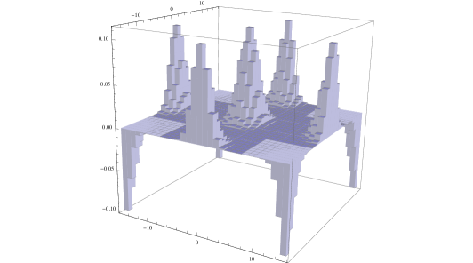
Figure 4: The Wigner function $W(n,m)$ in the case $\kappa=\frac{4}{3}$, $d\!=\!31$.

The shape of the functions involved in the expression (18) of $W$ can be seen in Figure 3. In the finite phase space (which is a finite torus), the obtained discrete Wigner function $W$ has three peaks placed around $(0,0)$, $(0,s)$, $(s,0)$ and an anti-peak around $(s,s)$ (see Figure 4). Note the similarity of the representation in Figure 4 and the results in [12, 16, 17].

The Wigner function from the continuous case is, in a certain sense, the limit of the discrete Wigner function. Therefore, in the continuous limit, the only“surviving” peak is expected to be that around $(0,0)$, in agreement with the known results from the Wigner function of continuous Gaussians. The disappearance of the peaks placed around $(0,s)$, $(s,0)$ and of the anti-peak around $(s,s)$ in the continuous limit is rather mysterious. The numerical simulations show that for large $d$ all of them keep an amplitude comparable to that of the peak placed around $(0,0)$. A possible explanation is the following. In finite dimension these peaks are placed on the “boundary” of the finite phase space $\mathcal{S}_{d}\times\mathcal{S}_{d}$. In the continuous limit they must be located on the “boundary” of the phase plane $\mathbb{R}^{2}$ which contains just one point, namely $\infty$. It is known that the compactification of the real or complex plane is obtained by adding one point, and the extended plane (called Riemann sphere) corresponds to the unit sphere through the stereographic projection. We can consider that, for $d\longrightarrow\infty$, that is, for $s\longrightarrow\infty$, the peaks placed around $(0,s)$, $(s,0)$ compensate with the anti-peak around $(s,s)$.

8 Discussions and Conclusions

The simpler way to define a Gaussian type function on the set $\{-s,-s\!+\!1,\,...\,,s\!-\!1,s\}$ or $\mathcal{S}_{d}$ is to consider the restriction of the Gaussian $g_{\kappa}(x)\!=\!\mathrm{e}^{-\frac{\kappa}{2}x^{2}}$ to these sets

$$f:\{-s,-s\!+\!1,\,...\,,s\!-\!1,s\}\longrightarrow\mathbb{R},\qquad f(n)={\rm e}^{-\frac{\kappa}{2}n^{2}}$$

respectively,

$$\begin{array}[]{l}f:\mathcal{S}_{d}\longrightarrow\mathbb{R},\qquad f\left(n\sqrt{\frac{2\pi}{d}}\right)={\rm e}^{-\kappa\frac{\pi}{d}n^{2}}.\end{array}$$

The functions obtained in this way behave similar to the continuous Gaussians only for large values of $d\!=\!2s\!+\!1$.

Our approach is based on an alternative method. By using a Weil-Zak type transform, we firstly generate a periodic function $G_{\kappa}$ with period $d$, and then we define our finite Gaussian as a restriction of $G_{\kappa}$ to $\mathbb{Z}$, namely $\mathfrak{g}(n)\!=\!G_{\kappa}(n)$. Our finite Gaussians starts to behave similar to a continuous Gaussian from relatively small values of $d$. In addition, they have several remarkable mathematical properties.

The discreteness of the configuration space has a particular appeal in both classical and quantum physics, particularly in phase space [18] or in attempts to unify general relativity and quantum mechanics [12]. On the other hand, the results in a discrete configuration space are required to match standard physical results in the continuum limit. Because discrete physical systems are of interest in quantum mechanics or in classical physics in connection to the problem of sampling, the characterization of such systems and of their evolution has already received some attention. For example, a discrete quantum phase space has been studied in [8, 9], the continuous limit being obtained by decreasing the lattice spacing in both momentum and position space, while in [2] the dynamics on a discrete quantum phase space has been investigated by defining a Hamiltonian with the appropriate classical limit. The results in this paper are different from previous ones and demonstrate the importance of the choice of some particular states in the discrete-continuum transition. As an additional example in this respect, we mention that a discrete model of the quantum harmonic oscillator, for instance, can be introduced such that the energy spectrum is equally-spaced and the spectra of both momentum and position operators are denumerable non-degenerate [1]. This last model, too, recovers the results for the ordinary harmonic oscillator in an appropriate limit. As do the discrete models of the quantum harmonic oscillator in terms of Kravchuk polynomials [10] or Harper functions [4].

Summarizing, the correct continuous limit of discrete models can be obtained in many situations. The choice of Gaussian states render the discrete-continuous transition smoother in the sense that many results known from the continuous case are obtained for reasonably large d values or can easily be extrapolated from the results for finite d values. Moreover, Gaussian states have advantages over other states in phase space representations of physical systems since, as shown in Section 7, the Wigner distribution function has a particularly simple expression in this case. In conclusion, finite Gaussian states represent a useful mathematical tool for the study of quantum or classical physical systems.

References

References

- [1] Atakishiyev N M, Klimyk A U and Wolf K B 2008 A discrete quantum model of the harmonic oscillator J. Phys. A: Math. Theor. 41 085201
- [2] Bang J Y and Berger M S 2006 Quantum mechanics and the generalized uncertainty principle Phys. Rev. D 74 125012
- [3] Bang J Y and Berger M S 2009 Wave packets in discrete quantum phase space Phys. Rev. A 80 1050
- [4] Barker L, Candan Ç, Hakioğlu T, Kutay M A and Ozaktas H M 2000 The discrete harmonic oscillator, Harper’s equation, and the discrete fractional Fourier transform J. Phys. A: Math. Gen. 33 2209
- [5] Cotfas N, Gazeau J P and Vourdas A 2011 Finite-dimensional Hilbert space and frame quantization J. Phys. A: Math. Theor. 44 175303
- [6] Floratos E G and Leontaris G K 1997 Uncertainty relation and non-dispersive states in finite quantum mechanics Phys.Lett. B 412 35-41
- [7] Gazeau J-P 2009 Coherent States in Quantum Physics (Berlin: Wiley-VCH)
- [8] Jagannathan R, Santhanam T S and Vasudevan R 1981 Int. J. Theor. Phys. 20 755
- [9] Jagannathan R and Santhanam T S 1982 Int. J. Theor. Phys. 21 351
- [10] Lorente M 2001 Continuous versus discrete models for the quantum harmonic oscillator and the hydrogen atom Phys. Lett. A 285 119
- [11] Magnus W, Oberhettinger F and Soni R P1966 Formulas and Theorems for the Special Functions of Mathematical Physics (New-York: Springer-Verlag)
- [12] Marchiolli M A and Ruzzi M 2012 Theoretical formulation of finite-dimensional discrete phase spaces: I. Algebraic structures and uncertainty principles Ann. Phys. 327 1538-1461
- [13] Marzoli I, Saif F, Bialynicki-Birula I, Friesch O M, Kaplan A E and Schleich W P 1998 Quantum carpets made simple Acta Phys. Slovaca 48 323
- [14] Massar S and Spindel P 2008 Uncertainty relation for the discrete Fourier transform Phys. Rev. Lett. 100 190401
- [15] Mehta M L 1987 Eigenvalues and eigenvectors of the finite Fourier transform J. Math. Phys. 28 781
- [16] Opatrný T, Buz̆ek V, Bajer J and Drobný G 1995 Propensities in discrete phase space: Q function of a state in a finite-dimensional Hilbert space Phys. Rev. A 52 2419
- [17] Opatrný T, Welsch D-G and Buz̆ek V 1996 Parametrized discrete phase-space functions Phys. Rev. A 53 3822
- [18] Poletti M A 1988 The development of a discrete transform for the Wigner distribution function J. Acoust. Soc. Am. 84 238
- [19] Ruzzi M 2006 Jacobi -functions and discrete Fourier transform J. Math. Phys. 47 063507
- [20] Štoviček P and Tolar J 1984 Quantum mechanics in discrete space-time Rep. Math. Phys. 20 157-70
- [21] Vilenkin N J and Klimyk A U 1992 Special Functions and Integral Transforms (Dordrecht: Kluwer Academic)
- [22] Vourdas A 2004 Quantum systems with finite Hilbert space Rep. Prog. Phys. 67 267-320
- [23] Weil A 1954 Sur certains groupes d’opérateurs unitaires Acta Math. 111 143-211
- [24] Whittaker E T and Watson G N 2000 Cambridge Mathematical Library: A Course of Modern Analysis (Cambridge: Cambridge University Press)
- [25] Wigner E P 1932 On the quantum correlation for thermodynamic equilibrium Phys. Rev. 40 749
- [26] Zak J 1967 Finite translations in solid state physics Phys. Rev. Lett. 19 1385
- [27] Zhang S and Vourdas A 2004 Analytic representation of finite quantum systems J. Phys. A: Math. Gen. 37 8349-63