A generalized Caroli formula for transmission coefficient with lead-lead coupling

Abstract

We present a generalized transmission coefficient formula for the lead-junction-lead system, in which interaction between the leads has been taken into account. Based on it the Caroli formula could be easily recovered and a transmission coefficient formula for interface problem in the ballistic system can be obtained. The condition of validity for the formula is carefully explored. We mainly focus on heat transport. However, the corresponding electrical transport could be similarly dealt with. Also, an illustrative example is given to clarify the precise meaning of the quantities used in the formula, such as the concept of the reduced interacting matrix in different situations. In addition, an explicit transmission coefficient formula for a general one-dimensional interface setup is obtained based on the derived interface formula.

I INTRODUCTION

In recent years there has been a huge increase in research and development of nanoscale science and technology, with the study of energy and electron transport playing important role. Focusing on thermal transport, Landauer-like results for steady-state heat flow have been proposed earlier Rego1998 ; Blencowe1999 . Subsequently, based on quantum Langevin equation approach, many authors successfully obtained a Landauer-type expression Segal2003 ; Dhar2006 ; Dhar2008 . Alternatively, nonequilibrium Green’s function (NEGF) method has been introduced to investigate mesoscopic thermal transport, which is particularly suited for use with ballistic thermal transport and readily allows the incorporation of nonlinear interactions Ozpineci2001 ; Wang2006 ; Galperin2007 . Generally speaking, in the lead-junction-lead system, steady-state heat current of ballistic thermal transport flowing from left lead to right lead has been described by the Landauer-like formula, which was derived first for electrical current, as

$$I= \int_{0}^{\infty}\frac{d\omega}{2\pi}\,\hbar\omega\,T\left[\omega\right]\left(f_{L}-f_{R}\right),$$ (1)

where $f_{\left\{L,R\right\}}=\left\{\exp\left({\hbar\omega}/{k_{B}T_{\left\{L,R\right\}}}\right)-1\right\}^{-1}$ is the Bose-Einstein distribution for phonons, and $T\left[\omega\right]$ is known as the transmission coefficient. Based on nonequilibrium Green’s function method, $T\left[\omega\right]$ can be calculated through the Caroli formula in terms of the Green’s functions of the junction and the self-energies of the leads,

$$T\left[\omega\right]= \mathrm{Tr}\left(G^{r}\Gamma_{R}G^{a}\Gamma_{L}\right),$$ (2)

where $G^{r,a}$ is the Green’s function of the junction, and

$$\Gamma_{\left\{L,R\right\}}= i\left[\Sigma_{\left\{L,R\right\}}^{r}-\Sigma_{\left\{L,R\right\}}^{a}\right],$$ (3)

where the self-energy terms $\Sigma^{r,a}_{\left\{L,R\right\}}$ are due to the semi-infinite leads on the left, $L$, and on the right, $R$, respectively. The superscript $r$ and $a$ denote the retarded and advanced, respectively, both for the self-energies as well as for the Green’s functions in the formula. The specific form (2) was given from NEGF formalism by Meir and Wingreen Meir1992 for electronic case and later by Yamamoto and Watanabe for phonon transport Yamamoto2006 , while Caroli et al. first obtained a formula for the electronic transport in a slightly more restricted case Caroli1971 . Also, Mingo et al. have derived a similar expression for transmission coefficient using “atomistic Green’s function” method Mingo2003 ; Zhang2007 . Very recently, Das and Dhar Suman2012 derive the Landauer-like expression from plane wave picture using Lippmann-Schwinger scattering approach.

The Landauer-like formula describes the situation in which the junction is small enough compared to the coherent length of the waves so that it could be treated as elastic scattering where the energy is conserved. Furthermore, it has been assumed that the two leads are decoupled which physically means there is no direct tunneling between the two leads. Through modern nanoscale technology, small junction is easily realized such as in certain nanoscale systems, for instance, a single molecule or, in general, a small cluster of atoms between two bulk electrodes. In that case, the electrode surfaces of the bulk conductors may be separated by just a few angstroms so that some finite electronic coupling between the two surfaces is inevitable taking into account the long-range interaction. In order to solve this problem, Di Ventra suggested that Ventra2008 we can choose our “sample” region (junction) to extend several atomic layers inside the bulk electrodes where screening is essentially complete so that the above coupling could be negligible. It turns out to be correct using this trick to avoid the interaction between the two leads, which will be verified in a simple example at the end of the paper, even though we, to some limited extent, modify the initial condition necessary to derive Landauer-like formula in NEGF formalism and repartition the total Hamiltonian. However, this procedure or trick could not be always done due to some topological reason such as studying heat current in Rubin model Rubin1971 in which the other end of the two semi-infinite leads is connected (a ring problem). Actually this somewhat trivial example is not so artificial since it is equivalent to using periodic boundary condition in Rubin model. Furthermore, the modification of the initial product state will certainly affect the behavior of the transient heat current. If we want to study the transient and steady heat current Bijay2011 in a unified way, the repartitioning procedure which changes the model is not acceptable. So in this work we will try to derive a compact formula applicable to this general model including lead-lead interaction for steady-state heat current according to NEGF formalism, and correspondingly obtained a Caroli-like formula for transmission coefficient. Furthermore, an interface transmission coefficient formula in the NEGF formalism will be given as a special case of the general Caroli-like formula. Also, the standard Caroli formula follows as a one-line proof.

The paper is organized into two main sections. In Section II, we develop our formalism to derive our generalized expression for the steady current directly taking coupling between leads into account. Based on this general formula, we will recover the Caroli formula and derive a computationally efficient interface formula in II.4. Then we apply this formalism to an illustrative model system in Section III and show the results of numerical calculations. Also, we will apply the interface formula obtained in Section II to derive an explicit expression for transmission coefficient in Section IV. Finally we conclude with a short discussion in Section V.

II FORMALISM

II.1 Model system

As was mentioned previously, we will consider the lead-junction-lead model initially prepared in product state $\hat{\rho}\left(t_{0}\right)=\frac{e^{-\beta_{L}H_{L}}}{\mathrm{Tr}\left(e^{-\beta_{L}H_{L}}\right)}\otimes\frac{e^{-\beta_{C}H_{C}}}{\mathrm{Tr}\left(e^{-\beta_{C}H_{C}}\right)}\otimes\frac{e^{-\beta_{R}H_{R}}}{\mathrm{Tr}\left(e^{-\beta_{R}H_{R}}\right)}$. We can imagine that left lead $\left(L\right)$, center junction $\left(C\right)$, and right lead $\left(R\right)$ in this model was in contact with three different heat baths at the inverse temperature $\beta_{L}\equiv\left(k_{B}T_{L}\right)^{-1}$, $\beta_{C}\equiv\left(k_{B}T_{C}\right)^{-1}$ and $\beta_{R}\equiv\left(k_{B}T_{R}\right)^{-1}$, respectively for time $t<t_{0}$. At time $t=t_{0}$, all the heat baths are removed, and coupling of the center junction with the leads and the interaction between the two leads are switched on abruptly. Now the total Hamiltonian of the lead-junction-lead system becomes

$$H_{tot}= H_{L}+H_{C}+H_{R}+H_{LC}+H_{CR}+H_{LR},$$ (4)

where $H_{\alpha}=\frac{1}{2}p_{\alpha}^{T}p_{\alpha}+$$\frac{1}{2}u_{\alpha}^{T}K^{\alpha}u_{\alpha},\;\alpha=L,C,R$ represents coupled harmonic oscillators, $u_{\alpha}\equiv\sqrt{m}x_{\alpha}$ and $p_{\alpha}$ are column vectors of transformed coordinates and corresponding conjugate momenta in region $\alpha$. The superscript $T$ stands for matrix transpose. $H_{LC}\equiv u_{L}^{T}V^{LC}u_{C}$ and $H_{CR}\equiv u_{C}^{T}V^{CR}u_{R}$ are the usual couplings between the junction and the two leads, which are certainly necessary to establish the heat current. Now the new term representing interaction between two leads $H_{LR}=u_{L}^{T}V^{LR}u_{R}$ will modify transmission coefficient greatly, which is our main interest.

It is worth mentioning that nonlinear interaction could be added inside the center junction and dealt with using self-consistent approach in the framework of NEGF, which has been done by many authors Ness2010 ; Xu2008 .

II.2 Steady state contour-ordered Green’s functions

Contour-ordered Green’s functions are the central objects in the NEGF formalism, among which the directly derived relation say, Dyson equation, could be readily transformed to all kinds of relations among the real-time Green’s functions by Langreth theorem Haug2008 . And many interesting quantities such as the current we will consider in the following subsection could be easily related to the proper real-time Green’s functions.

Steady-state contour-ordered Green’s functions are defined as

$$G_{jk}^{\alpha\beta}\left(\tau_{1},\tau_{2}\right)= -\frac{i}{\hbar}\mathrm{Tr}\left\{\hat{\rho}^{ss}\left(s\right)T_{c}\left[u_{j}^{\alpha}\left(\tau_{1}\right)u_{k}^{\beta}\left(\tau_{2}\right)\right]\right\},$$ (5)

where $\hat{\rho}^{ss}\left(s\right)=U\left(s,t_{0}\right)\hat{\rho}\left(t_{0}\right)U\left(t_{0},s\right)$ is the steady-state density operator, in which time $s>t_{0}$ introduced for convenience of later discussion could take any finite time since the switch-on time $t_{0}$ will be let to go to $-\infty$ at the end in order to establish steady-state heat current. $u_{j}^{\alpha}\left(\tau_{1}\right)=U\left(s,\tau_{1}\right)u_{j}^{\alpha}U\left(\tau_{1},s\right)$ is operator in the Heisenberg picture and similarly for $u_{k}^{\beta}\left(\tau_{2}\right)$. The variables $\tau_{1}$ and $\tau_{2}$ are on the contour from time $s$ to $\infty$ and back from $\infty$ to time $s$. $U\left(t_{0},s\right)$ etc. are the time evolution operators of the full Hamiltonian. $T_{c}$ is the contour-ordering super-operator. There is a strong assumption here which is all we need in the whole derivation, where we assume steady state could be established from initial product state after infinite time so that all the steady-state real-time Green’s function depend only on the difference of the two time arguments. This intuitively reasonable assumption is not always guaranteed and there is a specific example about how to establish steady-state heat current in Ref Cuansing2011 .

After $t_{0}\rightarrow-\infty$ , $s\rightarrow t_{0}^{+}$, and transforming to the interaction picture, where the total Hamiltonian $H_{tot}$ is separated into the free part $H_{0}=H_{L}+H_{C}+H_{R}$ and the interaction part $H_{int}=H_{LC}+H_{CR}+H_{LR}$, we obtain

$$G_{jk}^{\alpha\beta}\left(\tau_{1},\tau_{2}\right)=$$

$$-\frac{i}{\hbar}\mathrm{Tr}\left\{\hat{\rho}\left(-\infty\right)T_{c}\left[e^{-\frac{i}{\hbar}\int_{K}H_{int}^{I}\left(\tau^{\prime}\right)d\tau^{{}^{\prime}}}u_{I,j}^{\alpha}\left(\tau_{1}\right)u_{I,k}^{\beta}\left(\tau_{2}\right)\right]\right\},$$ (6)

where $u_{I,j}^{\alpha}\left(\tau_{1}\right)=e^{\frac{i}{\hbar}H_{0}\tau_{1}}u_{j}^{\alpha}e^{-\frac{i}{\hbar}H_{0}\tau_{1}}$ is operator in the interaction picture and similarly for $u_{I,k}^{\beta}\left(\tau_{2}\right)$ and $H_{int}^{I}\left(\tau^{\prime}\right)$. Now the variables $\tau_{1}$ and $\tau_{2}$ are on the Keldysh contour Schwinger-Keldysh ; Rammer1986 $K$ from $-\infty$ to $\infty$ and back from $\infty$ to $-\infty$. The contour variables such as $\tau_{1}$ only influence the ordering of the operators under $T_{c}$, and $e^{\frac{i}{\hbar}H_{0}\tau_{1}}$ has the same meaning as $e^{\frac{i}{\hbar}H_{0}t_{1}}$ with real time $t_{1}$. Expanding the exponential to perform a perturbation expansion and using Feynman diagrammatic technique, we can obtain Dyson equations for $G^{\alpha\beta}\left(\tau_{1},\tau_{2}\right),\;\alpha,\beta=L,C,R$ such as $G_{ij}^{CL}\left(\tau_{1},\tau_{2}\right)=\sum_{l,n}\int_{K}d\tau g_{il}^{C}\left(\tau_{1},\tau\right)V_{ln}^{CL}G_{nj}^{LL}\left(\tau,\tau_{2}\right)+\sum_{l,n}\int_{K}d\tau g_{il}^{C}\left(\tau_{1},\tau\right)V_{ln}^{CR}G_{nj}^{RL}\left(\tau,\tau_{2}\right)$, etc. All these Dyson equations could be symbolically lumped into a compact matrix expression,

$$G=g+gVG=g+GVg,$$ (7)

where $G=\begin{bmatrix}G^{LL}&G^{LC}&G^{LR}\\ G^{CL}&G^{CC}&G^{CR}\\ G^{RL}&G^{RC}&G^{RR}\end{bmatrix},$ $g=\begin{bmatrix}g^{L}&0&0\\ 0&g^{C}&0\\ 0&0&g^{R}\end{bmatrix},$ $V=\begin{bmatrix}0&V^{LC}&V^{LR}\\ V^{CL}&0&V^{CR}\\ V^{RL}&V^{RC}&0\end{bmatrix}$ ($V^{T}=V$), and

$$g_{jk}^{\alpha}\left(\tau_{1},\tau_{2}\right)=-\frac{i}{\hbar}\mathrm{Tr}\left\{\frac{e^{-\beta_{\alpha}H_{\alpha}}}{\mathrm{Tr}\left(e^{-\beta_{\alpha}H_{\alpha}}\right)}T_{c}\left[u_{I,j}^{\alpha}\left(\tau_{1}\right)u_{I,k}^{\alpha}\left(\tau_{2}\right)\right]\right\},$$ (8)

$\alpha=L,C,R$ are equilibrium contour-ordered Green’s functions for the free subsystems, which are easy to calculate directly. No approximation is needed here, since the coupling $H_{int}$ is quadratic.

II.3 Generalized steady-state current formula

Certainly, heat current flowing out of the left lead in steady state doesn’t depend on time and based on its definition $I_{L}^{ss}\equiv-\mathrm{Tr}\left[\hat{\rho}^{ss}\left(s\right){dH_{L}\left(t\right)}/{dt}\right]$ for $t>s$, we could simply obtain

$$I_{L}^{ss}= -\int_{-\infty}^{\infty}\frac{d\omega}{2\pi}\,\hbar\omega\,\mathrm{Tr}\left[\left(VG^{<}\left[\omega\right]\right)_{LL}\right]$$

$$= -\int_{-\infty}^{\infty}\frac{d\omega}{2\pi}\,\hbar\omega\,\mathrm{Tr}\left[\left(V_{red}G_{red}^{<}\left[\omega\right]\right)_{LL}\right],$$ (9)

where $\left(VG^{<}\left[\omega\right]\right)_{LL}$ denotes the $LL$ part submatrix of $VG^{<}\left[\omega\right]$. Observing the structure of $\mathrm{Tr}\left[\left(VG^{<}\left[\omega\right]\right)_{LL}\right]$, we note that the size of the $G^{<}\left[\omega\right]$ making nonzero contribution to $I_{L}^{ss}$ is completely determined by nonzero entries in the symmetric total coupling matrix $V$. So we don’t need the full $G^{<}\left[\omega\right]$ which is an infinite matrix due to the two semi-infinite leads. According to this observation, we choose the reduced square matrix $G_{red}^{<}\left[\omega\right]$ to be the corresponding submatrix of $G^{<}\left[\omega\right]$ determined by the row indexes of nonzero row vectors of coupling matrixes $V^{LC},V^{LR},V^{RC},V^{RL}$ plus full center part row indexes inside the total coupling matrix $V$ for the rows of $G_{red}^{<}\left[\omega\right]$, the column indexes of nonzero column vectors of coupling matrixes $V^{CL},V^{RL},V^{CR},V^{LR}$ plus full center part column indexes inside the total coupling matrix $V$ for the columns of $G_{red}^{<}\left[\omega\right]$. In order to calculate the lesser Green’s function $G_{red}^{<}\left[\omega\right]$, closed Dyson equation for reduced contour-ordered Green’s function $G_{red}\left(\tau_{1},\tau_{2}\right)$ is needed. Equation (7) is the starting point and indeed it is also true that $G_{red}=g_{red}+g_{red}V_{red}G_{red},$ where $g_{red}$ is similarly defined as $G_{red}$ and $V_{red}$ is the submatrix of original $V$ after crossing out all the zero column and row vectors except for the possible zero vectors whose row or column indexes are the center (junction) ones. Actually, $G_{red}$ is just the corresponding submatrix of $G$ just like $V_{red}$.

From now on, for notational simplicity, we omit the subscript $red$ of all the steady-state Green’s functions and all the coupling matrices with the understanding that these matrices are of finite dimensions.

Using the Langreth theorem Haug2008 and Fourier transforming the obtained all kinds of real-time Green’s functions, we can get

$$G^{<}\left[\omega\right]$$

$$= G^{r}\left[\omega\right]\begin{pmatrix}-if_{L}\tilde{\Gamma}_{L}\left[\omega\right]&0&0\\ 0&0&0\\ 0&0&-if_{R}\tilde{\Gamma}_{R}\left[\omega\right]\end{pmatrix}G^{a}\left[\omega\right],$$ (10)

where

$$\tilde{\Gamma}_{\left\{L,R\right\}}\equiv i\left[\left(g_{\left\{L,R\right\}}^{sur,a}\right)^{-1}-\left(g_{\left\{L,R\right\}}^{sur,r}\right)^{-1}\right],$$ (11)

$g_{L}^{sur,a}$ is the advanced surface Green’s function for the left lead coming from the corresponding part of the advanced reduced Green’s function $g_{red}^{a}$ and similarly for the retarded one. This new function plays important role for our generalized Caroli formula and for an interface formula to be derived below. Here, fluctuation dissipation theorem $g_{\alpha}^{<}\left[\omega\right]=f_{\alpha}\left[\omega\right]\left(g_{\alpha}^{r}-g_{\alpha}^{a}\right),\;\alpha=L,C,R.$ has been used. So is $\left(g_{C}^{a}\right)^{-1}-\left(g_{C}^{r}\right)^{-1}=0$, which is responsible for the vanishing of junction temperature dependence of final steady-state current formula. With respect to various Green’s functions and specific convention of Fourier transform, we use the same definitions as Ref. Wang2007 .

Substituting the Eq. (10) into steady current expression (9), we can easily obtain

$$I_{L}^{ss}= \int_{-\infty}^{\infty}\frac{d\omega}{2\pi}\,\hbar\omega\bigl{(}f_{L}T_{1}\left[\omega\right]+f_{R}T_{2}\left[\omega\right]\bigr{)},$$ (12)

Where,

$$T_{1}\left[\omega\right]=i\mathrm{Tr}\left(V^{LC}G_{CL}^{r}\tilde{\Gamma}_{L}G_{LL}^{a}+V^{LR}G_{RL}^{r}\tilde{\Gamma}_{L}G_{LL}^{a}\right),$$ (13)

$$T_{2}\left[\omega\right]=i\mathrm{Tr}\left(V^{LC}G_{CR}^{r}\tilde{\Gamma}_{R}G_{RL}^{a}+V^{LR}G_{RR}^{r}\tilde{\Gamma}_{R}G_{RL}^{a}\right),$$ (14)

Again applying Langreth theorem and Fourier transform to the corresponding reduced one of Eq. (7), we could get $G_{LR}^{a}=G_{LL}^{a}V^{LR}g_{R}^{sur,a}+G_{LC}^{a}V^{CR}g_{R}^{sur,a}$ and $G_{LC}^{a}=G_{LL}^{a}V^{LC}g_{C}^{a}+G_{LR}^{a}V^{RC}g_{C}^{a}$. Using the relations such as $\left(G_{CL}^{r}\right)^{\dagger}=G_{LC}^{a},\;\left(\tilde{\Gamma}_{L}\right)^{\dagger}=\tilde{\Gamma}_{L}$(where the superscript $\dagger$ stands for transpose conjugate) etc., we obtain

$$T_{1}\left[\omega\right]+T_{1}^{*}\left[\omega\right]= \mathrm{Tr}\left(G_{RL}^{r}\tilde{\Gamma}_{L}G_{LR}^{a}\tilde{\Gamma}_{R}\right),$$ (15)

In deriving it, cyclic property of the trace was used. Following similar steps, we could get

$$T_{2}\left[\omega\right]+T_{2}^{*}\left[\omega\right]= \mathrm{-Tr}\left(G_{RL}^{a}\tilde{\Gamma}_{L}G_{LR}^{r}\tilde{\Gamma}_{R}\right),$$ (16)

Due to these properties that $\tilde{\Gamma}_{\alpha}^{T}=\tilde{\Gamma}_{\alpha},\;\alpha=L,R$, $\left(G_{RL}^{r}\right)^{T}=G_{LR}^{r}$ and $\left(G_{RL}^{a}\right)^{T}=G_{LR}^{a}$, it is easy to show that $T_{1}+T_{1}^{*}=-\left(T_{2}+T_{2}^{*}\right).$ Now we define the general transmission coefficient

$$T_{G}\left[\omega\right]\equiv T_{1}\left[\omega\right]+T_{1}^{*}\left[\omega\right]=\mathrm{Tr}\left(G_{RL}^{a}\tilde{\Gamma}_{L}G_{LR}^{r}\tilde{\Gamma}_{R}\right).$$ (17)

Since current is certainly a real number, and this property has been kept in the whole derivation, we have $I_{L}^{ss}=\frac{1}{2}\left(I_{L}^{ss}+I_{L}^{ss*}\right)=\frac{1}{2}\int_{-\infty}^{\infty}\frac{d\omega}{2\pi}\,\hbar\omega\,T_{G}\left[\omega\right]\left(f_{L}-f_{R}\right)$.

According to the definitions of retarded and advanced Green’s functions in the frequency domain, we know $G_{RL}^{a}\left[-\omega\right]=\left(G_{LR}^{r}\left[\omega\right]\right)^{T}$and $\tilde{\Gamma}_{\left\{L,R\right\}}\left[-\omega\right]=\left(-\tilde{\Gamma}_{\left\{L,R\right\}}\left[\omega\right]\right)^{T}$. Together with $f_{L}\left[-\omega\right]-f_{R}\left[-\omega\right]=-f_{L}\left[\omega\right]+f_{R}\left[\omega\right]$, steady current $I_{L}^{ss}$ can be simplified further to the final expression

$$I_{L}^{ss}= \int_{0}^{\infty}\frac{d\omega}{2\pi}\,\hbar\omega\,T_{G}\left[\omega\right]\left(f_{L}-f_{R}\right).$$ (18)

Thus, it is the same as expected that Landauer-like formula still apply to this general case taking lead-lead interaction into account. And this Landauer-like formula with the explicit general transmission coefficient expression (17) is our central result.

Now we need to know how to calculate $G_{LR}^{r}$ in order for specific applications. According to the corresponding reduced one of Eq. (7), we can obtain a closed equation for $G_{LR}^{r}$

$$G_{LR}^{r}= \tilde{g}_{L}^{r}\tilde{V}^{LR,r}\tilde{g}_{R}^{r}+\tilde{g}_{L}^{r}\tilde{V}^{LR,r}\tilde{g}_{R}^{r}\tilde{V}^{RL,r}G_{LR}^{r},$$ (19)

where $\tilde{g}_{\alpha}^{r}\equiv\left(\left(g_{\alpha}^{sur,r}\right)^{-1}-V^{\alpha C}g_{C}^{r}V^{C\alpha}\right)^{-1},\;\alpha=L,R$, and $\left(\tilde{V}^{RL,r}\right)^{T}=\tilde{V}^{LR,r}=V^{LR}+V^{LC}g_{C}^{r}V^{CR}$. Since $G_{RL}^{a}=\left(G_{LR}^{r}\right)^{\dagger}$, now all the quantities necessary to obtain general transmission coefficient $T_{G}$ could be expressed in terms of retarded or advanced form of submatrix of $g_{red}$ and submatrix of $V_{red}$, which are both easily obtained.

II.4 Recovering Caroli formula and deriving an interface formula

First, we recover Caroli formula for transmission coefficient. In this case, coupling between the two leads $V_{LR}$ has been assumed to be $0$. Thus, similar to what we did in subsection II.3, we could easily derived $G_{LR}^{r}=g_{L}^{sur,r}V^{LC}G_{CR}^{r}=g_{L}^{sur,r}V^{LC}G_{CC}^{r}V^{CR}g_{R}^{sur,r}$. Together with $G_{RL}^{a}=\left(G_{LR}^{r}\right)^{\dagger}$, we could immediately obtain from formula (17) that $T\left[\omega\right]=\mathrm{Tr}\left(G_{CC}^{r}\Gamma_{R}G_{CC}^{a}\Gamma_{L}\right)$. Here, we should remember that all the quantities inside the trace now are reduced ones. However, it is still equal to expression (2), in which all the quantities could be the full ones, taking trace operation and the reducing procedure for $G$ and $V$ into account. How to calculate $T\left[\omega\right]$ and apply this efficient formula to specific applications has been stated by many authors, e.g. Wang2008 .

Now we try to derive an interface formula still based on formula (17). By interface we simply mean left lead and right lead has been connected directly and center junction has been removed. Mathematically, we know $V^{CL}=0$ and $V^{CR}=0$ in this situation. Consequently, $G_{LR}^{r}=g_{L}^{sur,r}V^{LR}G_{RR}^{r}$ and $G_{RL}^{a}=\left(G_{LR}^{r}\right)^{\dagger}=G_{RR}^{a}V^{RL}g_{L}^{sur,a}$. Straightforwardly, we get the transmission coefficient formula in this interface problem Bijay2012

$$T_{I}\left[\omega\right]= \mathrm{Tr}\left(G_{RR}^{r}\tilde{\Gamma}_{R}G_{RR}^{a}\Gamma_{L}\right).$$ (20)

In order to apply this formula, still we need a closed equation for $G_{RR}^{r}$, which could be simply obtained to be

$$G_{RR}^{r}= g_{R}^{sur,r}+g_{R}^{sur,r}\tilde{\Sigma}_{L}^{r}G_{RR}^{r},$$ (21)

where the reduced retarded self-energy is given by $\tilde{\Sigma}_{L}^{r}=V^{RL}g_{L}^{sur,r}V^{LR}$.

III AN ILLUSTRATIVE APPLICATION

The illustrative example is a one-dimensional central ring problem, in which there is only one particle in the center junction connected with two semi-infinite spring chain leads. In this model, the interaction between the two nearest particles inside the two leads also exists taken into account as $V^{LR}$. Thus, the form of the total Hamiltonian is the same as (4) with $K_{0}^{\alpha},\;\alpha=L,R$ the semi-infinite tridiagonal spring constant matrix consisting of $2\omega_{1}^{2}+\omega_{0}^{2}$ along the diagonal and $-\omega_{1}^{2}$ along the two off-diagonals, $K^{C}=2\omega_{1}^{2}+\omega_{0}^{2}$, $V_{red}^{LC}=-\omega_{1}^{2}$, $V_{red}^{CR}=-\omega_{1}^{2}$ and $V_{red}^{LR}=-\beta\omega_{1}^{2}$, where $\beta$ is the coupling strength between two leads. The on-site potential term $\omega_{0}^{2}$ is necessary in establishing the steady-state current dynamically Cuansing2011 . In this simple case, there is an analytical expression for $g_{\alpha,0}^{sur,r}\left[\omega\right],\;\alpha=L,R$, which is $g_{\alpha,0}^{sur,r}=-{\lambda_{1}}/{\omega_{1}^{2}}$, $\lambda_{1}=(-\Omega\pm\sqrt{\Omega^{2}-4\omega_{1}^{4}})/(2\omega_{1}^{2})$, where $\Omega=\left(\omega+i0^{+}\right)^{2}-2\omega_{1}^{2}-\omega_{0}^{2}$ and the choice between the plus or minus sign depends on satisfying $\left|\lambda_{1}\right|<1$. And $g_{C}^{sur,r}\left[\omega\right]={1}/{\Omega}$. After all these preparations, the transmission coefficient is simply calculated by the formula (17).

Also, there is an alternative method to deal with this problem suggested by Di Ventra as we mentioned in Section I. Essentially we repartition the total Hamiltonian so that interaction between leads is absent. Thus, in this model, the form of the total Hamiltonian is still the same as (4) but with

$$K^{C}= \begin{bmatrix}2\omega_{1}^{2}+\omega_{0}^{2}&-\omega_{1}^{2}&-\beta\omega_{1}^{2}\\ -\omega_{1}^{2}&2\omega_{1}^{2}+\omega_{0}^{2}&-\omega_{1}^{2}\\ -\beta\omega_{1}^{2}&-\omega_{1}^{2}&2\omega_{1}^{2}+\omega_{0}^{2}\end{bmatrix},$$ (22)

$$V_{red}^{LC}= \begin{bmatrix}-\omega_{1}^{2}&0&0\end{bmatrix},$$ (23)

$$V_{red}^{CR}= \begin{bmatrix}0\\ 0\\ -\omega_{1}^{2}\end{bmatrix}.$$ (24)

Since now $V_{red}^{LR}=0$, we can use either the Caroli formula (2) or the general one (17) to calculate the transmission coefficient. The results of the two methods were compared in Fig. 1. It turns out to be that they are the same, which justifies the suggestion of Di Ventra from NEGF point of view in this example.

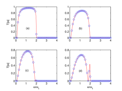
Figure 1: (Color online) The transmission coefficient $T\left[\omega\right]$ as a function of frequency for coupling between leads (a) $\beta=0.2$, (b) $\beta=0.4$, (c) $\beta=0.6$, (d) $\beta=0.8$. The results was calculated directly (red solid line), and by repartitioning the total Hamiltonian (blue circles). $\omega_{0}=0.1\,\omega_{1}$ in all cases.

Probably a much efficient way to calculate the transmission coefficient in this type of noninteracting problem is to use the interface formula (20). Frequently, the surface Green’s functions will become complex when we separate the total system into two parts in order to apply the interface formula. However, there are some efficient algorithms for surface Green’s functions see, for example, Ref. Wang2008 . Now we will show a specific application of interface formula (20).

IV an explicit interface transmission function formula

Here in this section we derive an explicit expression for the transmission function $T_{I}[\omega]$ using Eq. (20) for the single interface setup, i.e. the left and right lead are directly connected and the center part is removed.

Let us consider that the normalized force constant for left and the right leads are $\omega_{1}^{2}$ and $\omega_{2}^{2}$ respectively and the normalized interface coupling strength is $\omega_{12}^{2}$. Also, onsite potential $\omega_{0}^{2}$ to all the atoms exists to ensure that the steady state could be established dynamically. This is a quite general scenario for a one-dimensional harmonic chain which is useful for the study of interface effects. So one of the force constant matrix say $K^{L}$ is equal to $K_{0}^{L}+\Delta K$ where $\Delta K$ is the semi-infinite matrix with only first element is nonzero $\Delta K_{11}=\omega_{12}^{2}-\omega_{1}^{2}$ while $K_{0}^{L}$ is the same as defined in the last application. Similarly for $K^{R}$ with $\omega_{1}^{2}$ replaced by $\omega_{2}^{2}$. In order to obtain the explicit form, only inputs that are required are retarded surface Green’s function $g_{\alpha}^{sur,r}$ for both the leads. $G_{RR}^{\left\{r,a\right\}}$ in Eq. (20) can then be easily obtained from these expressions.

Let us calculate the surface Green’s function for one of the leads, say the left lead. Then for the right lead it can be obtained just by replacing $\omega_{1}^{2}$ with $\omega_{2}^{2}$. The surface Green’s function for a semi-infinite lead when all force constants are the same is given as before, i.e. $g_{L,0}^{sur,r}$. Now for this interface case we can obtain the surface Green’s function as follows. The retarded Green’s function for the left lead satisfies the following equation

$$\big{[}(\omega+i0^{+})^{2}-K^{L}\big{]}g_{L}^{r}=I.$$ (25)

Taking $K^{L}=K_{0}^{L}+\Delta K$ into account, and using $\Delta K$ as a perturbation we can write

$$g_{L}^{r}=g_{L}^{r,0}+g_{L}^{r,0}\Delta Kg_{L}^{r}.$$ (26)

Since in this case only first atom of the left lead is connected with the first atom of the right lead, the retarded surface Green’s function of the left lead is just the $(1,1)^{\rm th}$ element of $g_{L}^{r}$ and we obtain

$$g_{L}^{sur,r}=\frac{1}{\omega_{1}^{2}-\omega_{12}^{2}-\omega_{1}^{2}/\lambda_{1}},$$ (27)

and the self-energy for the lead is given by

$$\tilde{\Sigma}_{L}^{r}=\frac{\omega_{12}^{4}}{\omega_{1}^{2}-\omega_{12}^{2}-\omega_{1}^{2}/\lambda_{1}}.$$ (28)

Knowing this surface Green’s function and self-energy, we can easily obtain ${T_{I}}[\omega]$ from Eq. (20) which can be written as

$${T_{I}}[\omega]=-\frac{\omega_{1}^{2}\omega_{2}^{2}\omega_{12}^{4}(\lambda_{1}-\lambda_{1}^{*})(\lambda_{2}-\lambda_{2}^{*})}{\big{|}(\omega_{1}^{2}-\omega_{12}^{2}-\omega_{1}^{2}/\lambda_{1})(\omega_{2}^{2}-\omega_{12}^{2}-\omega_{2}^{2}/\lambda_{2})-\omega_{12}^{4}\big{|}^{2}},$$ (29)

where, $\lambda_{2}$ is similarly defined as $\lambda_{1}$ with $\omega_{1}$ replaced by $\omega_{2}$. It has been noted that it matches exactly with the result in Ref. Zhang2011 , where this expression is obtained from wave-scattering method. Now if $\omega_{1}^{2}=\omega_{2}^{2}=\omega_{12}^{2}$ then we have perfect transmission i.e., ${T_{I}}[\omega]=1$ for $\omega$ within the phonon band $\omega_{0}^{2}\leq\omega^{2}\leq 4\omega_{1}^{2}+\omega_{0}^{2}$ and $0$ outside this region.

V SUMMARY

We examine the heat current in a lead-junction-lead quantum system, in which coupling between the leads has been taken into account. After assuming ideal steady state could be established from initial product state, we rigorously derived a general Landauer-like formula in the NEGF framework, from which the corresponding transmission coefficient was obtained. Based on this general transmission coefficient formula, Caroli formula was recovered and a computationally efficient interface formula applicable to the case in which the total noninteracting Hamiltonian could be repartitioned was derived. Also an illustrative example was given as both a verification of the validity of the repartitioning procedure which doesn’t affect the steady current value and the clarification of the meaning of some quantities used in the formula such as $V_{red}^{LC}$ etc in different situations. Finally, we derived an explicit transmission coefficient formula in a quite general one-dimensional interface situation based on interface formula, which turned out to be perfectly consistent with result obtained by wave-scattering method.

References

• (1) L. G. C. Rego and G. Kirczenow, Phys. Rev. Lett. 81, 232, (1998).
• (2) M. P. Blencowe, Phys. Rev. B 59, 4992 (1999).
• (3) D. Segal, A. Nitzan, and P. Hänggi, J. Chem. Phys. 119, 6840 (2003).
• (4) A. Dhar and D. Roy, J. Stat. Phys. 125, 805 (2006).
• (5) A. Dhar, Adv. in Phys., 57, 457-537 (2008).
• (6) A.Ozpineci and S. Ciraci, Phys. Rev. B 63, 125415 (2001).
• (7) J.-S. Wang, J. Wang, and N. Zeng, Phys. Rev. B 74, 033408 (2006).
• (8) M. Galperin, A. Nitzan, and M. A. Ratner, Phys. Rev. B 75, 155312 (2007).
• (9) Y. Meir and N. S. Wingreen, Phys. Rev. Lett. 68, 2512 (1992).
• (10) T. Yamamoto and K. Watanabe, Phys. Rev. Lett. 96, 255503 (2006).
• (11) C. Caroli, R. Combescot, P. Nozieres, D. Saint-James, J. Phys. C: Solid St. Phys. 4, 916 (1971).
• (12) N. Mingo, L. Yang, Phys. Rev. B 68, 245406, (2003).
• (13) W. Zhang, T. S. Fisher, and N. Mingo, Numer. Heat Transf. Part B, 51, 333 (2007).
• (14) S. G. Das and A. Dhar arXiv:1204.5595.
• (15) M. Di. Ventra, Electrical Transport in Nanoscale Systems, Cambridge University Press, 2008.
• (16) R. J. Rubin and W. L. Greer, J. Math. Phys. 12, 1686 (1971).
• (17) J.-S. Wang, B. K. Agarwalla, and H. Li, Phys. Rev. B 84, 153412, (2011).
• (18) H. Ness, L. K. Dash, and R. W. Godby, Phys. Rev. B 82, 085426 (2010).
• (19) Y. Xu, J.-S. Wang, W. Duan, B.-L. Gu, and B. Li, Phys. Rev. B 78, 224303 (2008).
• (20) H. Haug and A.-P. Jauho, Quantum Kinetics in Transport and Optics of Semiconductors, 2nd ed. (Springer, New York, 2008).
• (21) E. C. Cuansing, H. Li, and J.-S. Wang, arXiv:1105.2233.
• (22) J. Schwinger, J. Math. Phys. 2, 407 (1961); L.V. Keldysh, Sov. Phys. JETP 20, 1018 (1965).
• (23) J. Rammer and H. Smith, Rev. Mod. Phys. 58, 323 (1986).
• (24) J.-S. Wang, N. Zeng, J. Wang, and C. K. Gan, Phys. Rev. E 75, 061128 (2007).
• (25) J.-S. Wang, J. Wang, and J. T. Lü, Eur. Phys. J. B 62, 381 (2008).
• (26) B. K. Agarwalla, J.-S. Wang, and B. Li, Unpublished.
• (27) L. Zhang, P. Keblinski, J.-S. Wang, and B. Li, Phys. Rev. B 83, 064303 (2011).