Pulsar data analysis with psrchive

Abstract

psrchive is an open-source, object-oriented, scientific data analysis software library and application suite for pulsar astronomy. It implements an extensive range of general-purpose algorithms for use in data calibration and integration, statistical analysis and modeling, and visualisation. These are utilised by a variety of applications specialised for tasks such as pulsar timing, polarimetry, radio frequency interference mitigation, and pulse variability studies. This paper presents a general overview of psrchive functionality with some focus on the integrated interfaces developed for the core applications.

1 Introduction

Within the pulsar astronomy community, a number of individuals and research groups have developed freely-available software for a wide variety of purposes. The sigproc (Lorimer, 2001) and presto (Ransom et al., 2002, 2003) software packages are widely used in the search for new pulsars, dspsr enables real-time phase-coherent dispersion removal (van Straten & Bailes, 2011) and computation of the cyclic spectrum (Demorest, 2011), both tempo (Taylor & Weisberg, 1989) and tempo2 (Edwards et al., 2006) are used in the analysis of pulse arrival time estimates, and psrcat provides access to the ATNF Pulsar Catalog (Manchester et al., 2005). This paper describes some of the basic and advanced functionality of the psrchive project, which provides access to a comprehensive range of tools commonly required for the analysis of pulse profile data and the various metadata that describe them (Hotan et al., 2004).

Each of the above software projects has been refined through stages of early adoption and beta testing followed by more regular usage and feedback from the community. In turn, as the software grows more reliable and reputable, it reduces barriers to newcomers, thereby promoting growth in the discipline. These tools are now an indispensable resource to researchers in the field, and nearly all observational analyses of radio pulsar data published in the past few decades have relied on one or more of these packages.

Many of the most fundamental algorithms implemented by psrchive originate in the timing analysis software developed by the collaborators of the Parkes Southern Pulsar Survey (PSPS; Manchester et al., 1996). Over nearly two decades, these have been generalized, refined and incorporated into a modular and extensible framework that employs object-oriented design principles and is primarily implemented using the C++ language. To increase the portability of the code, it is currently managed using an open-source distributed version control system and compiled using a cross-platform build system.

psrchive was developed in parallel with the psrfits file format, which is fully compliant with the Flexible Image Transport System (FITS; Hanisch et al., 2001) endorsed by NASA and the IAU and compatible with the recommendations of the International Virtual Observatory Alliance. The modular, object-oriented design of the psrchive software separates the data analysis routines from file I/O, enabling the software to be easily extended to handle other data formats. In addition to maintaining backward-compatibility with the file format used by the original PSPS timing analysis software, psrchive currently provides support to read data in eight different formats, including the European Pulsar Network flexible format (Lorimer et al., 1998), the presto prepfold output format, and three different file formats used by pulsar instruments at the Arecibo Observatory. psrchive automatically determines the format of input data files, and all of the usage examples presented in this paper can be applied to any of the supported formats without modification.

The portability and extensibility of psrchive fosters the incorporation of new features and functionality, including rigorous polarimetric calibration (van Straten, 2004; Ord et al., 2004); various methods of arrival time estimation (e.g. Taylor, 1992; Hotan et al., 2005; van Straten, 2006); Faraday rotation measure determination (Han et al., 2006; Noutsos et al., 2008); propagation of the fourth-order moments of the electric field (van Straten, 2009); and statistical analysis of profile variability (Demorest, 2007; Osłowski et al., 2011). Development also continues on some of the more elementary algorithms, such as estimation of the off-pulse baseline and identification of the on-pulse region, and computation of the signal-to-noise ratio.

The functionality of psrchive is distributed across a suite of specialised programs that are run from the command line in a typical UNIX shell environment. A subset of these programs, known as the Core Applications, provide access to general-purpose routines that are typically required for the majority of data analyses; these include

• psredit - queries or modifies the metadata that describe the data set;

• psrstat - derives statistical quantities from the data set and evaluates mathematical expressions;

• psrsh - command language interpreter used to transform and reduce data sets; and

• psrplot - produces customized, diagnostic and publication-quality plots.

The Core Applications employ a standard set of command line options and incorporate a command language interpreter that can evaluate mathematical and logical expressions, compute various statistical quantities, and execute a number of algorithms implemented by psrchive. Using the Core Applications and data that are available for download from the CSIRO Data Access Portal, this paper demonstrates a typical scientific workflow used to analyse observational data and produce pulse arrival time estimates for high-precision timing. As part of this demonstration, psrchive is used to perform radio frequency interference (RFI) excision, polarimetric calibration, and statistical bias correction. Throughout the paper, reference is made to the more extensive online documentation available at the psrchive web site. Detailed usage information is also output by each program via the -h command-line option. In sections 2 through 5, each Core Application is introduced with a description of the motivation and design of the program followed by a demonstration of its use through a practical exercise. Sections 6 through 8 demonstrate the use of psrchive to perform RFI mitigation, polarimetric calibration, arrival time estimation and bias correction. The concluding remarks in Section 9 include a description of some psrchive functionality that is currently under development and some ideas for future work.

1.1 Observational Data

The psrchive software processes observational data stored as a three-dimensional array of pulse profiles; the axes are time (sub-integration), frequency (channel), and polarization (e.g. the four Stokes parameters). The physical properties of the data are described by various attributes (also called metadata). A single data file containing one or more sub-integrations is typically called an archive. Sub-integration lengths may be as short as one pulse period (e.g. for single-pulse studies) or as long as desired (e.g. for the standard, or template profile, used for high-precision timing).

The examples in this paper make use of nine days of observations of PSR J0437$-$4715 made at 20 cm with the Parkes 64 m radio telescope on 19 to 27 July 2003. Discovered in the Parkes 70-cm survey (Johnston et al., 1993), PSR J0437$-$4715 remains the closest and brightest millisecond pulsar known; it has a spin period of $\sim 5.7$ ms, a pulse width of about 130 $\mu$s (Navarro et al., 1997) and an average flux of 140 mJy at 20 cm (Kramer et al., 1998). With a sharply-rising main peak and large flux density, it is an excellent target for high-precision pulsar timing studies. However, owing to the transition between orthogonally polarized modes of emission near the peak of the mean pulse profile, arrival time estimates derived from observations of PSR J0437$-$4715 are particularly sensitive to instrumental calibration errors (Sandhu et al., 1997; van Straten, 2006). Furthermore, pulse-to-pulse fluctuations in the emission from this pulsar on timescales ranging from $\sim 10$ to $\sim 300$ $\mu$s (Jenet et al., 1998) place a fundamental limit on the timing precision that can be achieved (Osłowski et al., 2011). These issues are discussed in more detail in Sections 7 and 8, which demonstrate the psrchive tools available for mitigating the impact of polarization calibration errors and correcting the bias due to self-noise.

As described in the Appendix, these data are available for download from the CSIRO Data Access Portal using the Pulsar Search tool. A significantly reduced and more readily accessible form of the data is also available for download from Swinburne University of Technology. Throughout this paper, it is assumed that the full path to the directory containing the observational data downloaded from Swinburne is recorded using the $PSRCHIVE_DATA shell environment variable.

2 Query and modify metadata with psredit

The pulse profile data stored in a pulsar archive file are accompanied by metadata, or attributes, that describe various physical characteristics of the observation such as the source name, right ascension and declination, centre radio frequency and bandwidth of the instrument, start time and duration of the integration, etc. These attributes may be queried and modified using the psredit program, which is more fully documented online.

The keywords used by psredit to address the attributes in an archive are also understood and used by other Core Applications. For example, using psredit keywords, psrstat can perform variable substitution and evaluate mathematical expressions that include attribute values; similarly, psrplot can annotate plots (e.g. axes labels and titles) with attribute values as well as any of the mathematical expressions and statistical quantities provided by psrstat. This modularity of design allows the interfaces to the Core Applications to be remembered once and used often.

Exercise: In the $PSRCHIVE_DATA/mem directory, the receiver name is not set in any of the data files (*.ar). This can be verified by querying the receiver name attribute.

     cd $PSRCHIVE_DATA/mem  psredit -c rcvr:name *.ar     Running psredit <filename> with no arguments will print a listing of every attribute in the file. Attribute names that end in an asterisk (e.g. int*:wt*) represent vector quantities. Specifying the attribute name without the asterisk will print a comma-separated list of every element in the vector; e.g. to print the centre frequency of every channel in every sub-integration

     psredit -c int:freq *.ar     (These data files contain 1 sub-integration and 128 frequency channels.) To query the value of a single element, or range of elements, a simple array syntax can be used; e.g.

     psredit -c ’int:freq[34,56-60]’ *.ar     will print only 6 values for each file. The single quotation marks in the above command are necessary to protect the square brackets from interpretation by the shell.

Set the receiver name to MULT_1 using the standard output option to overwrite the original files.

     cd $PSRCHIVE_DATA/mem  psredit -c rcvr:name=MULT_1 -m *.ar     The data files in $PSRCHIVE_DATA/mem/ are a mixture of three different types. Create two sub-directories called pulsar/ and cal/ then use psredit to query the type attribute and use this to sort the files into the two sub-directories.

     cd $PSRCHIVE_DATA/mem  mkdir pulsar/  mkdir cal/  mv `psredit -c type *.ar | grep Pulsar | awk ’{print $1}’` pulsar/  mv *.ar cal/     The last line of the above commands places all three calibrator file types in the cal/ sub-directory.

3 Evaluate data with psrstat

In addition to accessing the physical attributes that describe the observation, it is also useful to compute derived quantities, such as statistical measures that describe the quality of the data, the effective width of the pulse, the degree of polarisation, etc. A wide variety of derived quantities can be computed using the psrstat program, which is more fully documented online. Running psrstat <filename> without any command-line arguments will print a listing of every available quantity.

Any of the quantities (attributes or computed values) provided by the psrstat interface can be substituted into mathematical expressions that can be evaluated (expressions to be evaluated are enclosed in braces). For example, to search for significant peaks in a series of single-pulse archives, query the maximum amplitude in all phase bins normalized by the off-pulse standard deviation,

     psrstat -c ’{$all:max/$off:rms}’ <filenames>     To query the effective pulse width in microseconds,

     psrstat -c ’{$weff*$int[0]:period*1e6}’ <filename>     

Exercise: Use psrstat to print the signal-to-noise ratio, $S/N$, of each of the pulsar observations.

     psrstat -c snr pulsar/*.ar     Note that, by default, psrstat computes the $S/N$ of the profile in the first sub-integration, frequency channel and polarization (indexed by subint, chan and pol, respectively). Take one file and print the $S/N$ in each frequency channel using the command line option to loop over an index. The number of frequency channels in the file can be queried with the nchan attribute.

     psredit -c nchan pulsar/n2003200180804.ar  psrstat -l chan=0-127 -c snr pulsar/n2003200180804.ar     The psrstat program can be used in combination with other common tools (such as gnuplot) to investigate problems and/or verify the quality of data. When doing so, it is practical to use the -Q command line option to print only the value of each attribute, instead of key=value.

4 Transform and reduce data with the psrsh interpreter

psrchive includes a command language interpreter that provides access to a large number of common data processing algorithms, including radio frequency interference mitigation and polarimetric calibration. Access to this interpreter is provided by the psrsh program, which may be used either as an interactive shell environment or as a shell script command processor as more fully documented online.

The psrsh interpreter is also embedded in the command line interfaces of the Core Applications (psrstat, psrplot, and psradd). These applications use the interpreter to execute preprocessing tasks on input data files as described in Section 2.3 Job preprocessor of the online documentation. The full list of available commands is listed by running psrsh -H. The first column of the output is the command name, the second column is a single-letter short-cut key in square brackets, and the third column is a short description of each command.

Exercise: The $S/N$ values output by psrstat in the previous section are those of only one polarization, not the total intensity. The four polarization parameters stored in these files describe the elements of the coherency matrix: $AA$, $BB$, $\Re[AB]$, and $\Im[AB]$. The total intensity, $I=AA+BB$ is formed by the pscrunch command. Use the preprocessing capability of psrstat to print the $S/N$ of the total intensity as a function of frequency for one file.

     psrstat -j pscrunch -l chan=0-127 -c snr pulsar/n2003200180804.ar     Add the fscrunch command to print the $S/N$ of the total intensity integrated across the entire observing bandwidth for each file.

     psrstat -j pscrunch,fscrunch -c snr pulsar/*.ar     Using single-letter short-cut keys, the above line is equivalent to

     psrstat -j pF -c snr pulsar/*.ar     The output of the above command (combined with the -Q command line option) can be redirected to a file and gnuplot can be used to plot the variation of $S/N$ as a function of time due to interstellar scintillation.

5 Display data with psrplot

Using the pgplot graphics subroutine library, psrplot produces both diagnostic and publication-quality plots as documented online. The psrplot program is a highly configurable plotting tool for use during all stages of data analysis and manuscript preparation. To see a full listing of available plot types, use the -P command-line option. Each plot can be configured using a wide range of options, including selection of the range of data to be plotted (zooming), specification of plotting attributes such as character size and line width, and definition of plot labels. Run psrplot -A <name> to list the generic options that are common to most plots, and psrplot -C <name> to list the options that are specific to the named plot.

Plot labels may include any of the attributes accessible via psredit and/or quantities and mathematical expressions computed by psrstat. For example, to produce a publication-quality plot of the total intensity profile with the $S/N$ printed inside the top-right corner of the plot frame,

     psrplot <filename> -pD -jFp -c below:r=’S/N: $snr’ -c set=pub     Note that filename(s) need not necessarily be the last argument(s) on the command line.

Exercise: Use psrplot to plot the phase-vs-frequency image of the total intensity of the pulsar signal in each file.

     psrplot -p freq -j p pulsar/*.ar     By default, the dispersion delays between frequency channels are not corrected. Using the command line option to loop over an index, plot the phase-vs-frequency images of $\Re[AB]$ and $\Im[AB]$ (pol=2,3), which effectively correspond to Stokes $U$ and $V$.

     psrplot -p freq -l pol=2,3 pulsar/*.ar     These quantities vary with frequency due to an instrumental effect; the two orthogonal polarizations propagate through different signal paths with slightly different lengths, introducing a phase delay that varies linearly with radio frequency.

Use the loop-over-index option to plot the total intensity profile (the plot type named flux or its short-cut D) as a function of frequency in one pulsar data file.

     psrplot -pD -l chan=0- -jp pulsar/n2003200180804.ar     Note that chan=0- specifies the entire range without having to know the index of the last frequency channel. The pulse profile is significantly distorted at the edges of the band due to quantization error (also called “scattered power”) that arises during analog-to-digital conversion using 2 bits/sample. The most severely affected channels will be excised in Section 6.

Plot the Stokes parameters integrated over all frequency channels for each file.

     psrplot -p stokes -jF pulsar/*.ar     The white line is the total intensity; red, green, and blue correspond to Stokes $Q$, $U$, and $V$, respectively. The Stokes parameters vary with time owing to the rotation of the receiver feed with respect to the sky (the parallactic angle). In Section 7, this effect will be exploited to model the polarization cross-coupling in the instrumental response and calibrate the data.

6 Radio Frequency Interference and Invalid Data Excision

In the typical analysis of observational data, it is necessary to discard samples that have been corrupted by experimental error, instrumental distortion, and/or radio frequency interference. This section demonstrates some of the psrchive algorithms that are available to assist in the automatic detection and excision of corrupted data.

6.1 Excision of frequency channels that are known to be corrupted

Although the observations of PSR J0437$-$4715 used in this paper are not adversely affected by radio frequency interference, the data near the edges of the band are known to be corrupted by quantization distortions.

Exercise: Use the psrsh command language interpreter and the zap edge command to assign zero weight to 15% of the total bandwidth ($\sim 19$ frequency channels) on each edge of the band. Use the output option to write output data files with a new extension; e.g.

     cd $PSRCHIVE_DATA/mem  psrsh - -e zz pulsar/*.ar cal/*.ar << EOD  zap edge 0.15  EOD     In the above example, the single hyphen (-) command-line option instructs psrsh to read the command script from the standard input.

6.2 Automatic detection and excision of narrow-band interference

Many types of radio frequency interference (RFI) are narrow band, such that the quality of an observation can be significantly improved by discarding only a small number of corrupted frequency channels. The RFI environment at the telescope may be dynamic, such that it is not possible to select a fixed set of frequency channels to be excised at all times. To address this problem, psrchive implements an automatic frequency channel excision algorithm that is based on tolerance to differences between the observed spectrum and a version of the spectrum that has been smoothed by a running median. By default, the running median is computed using a window that is 21 frequency channels wide and all channels with total flux that differs from the median-smoothed spectrum by more than 4 times the standard deviation will be given zero weight. The standard deviation is defined recursively. That is, the algorithm works as follows

1. compute median-smoothed spectrum

2. compute standard deviation, ignoring any zapped channels

3. zap channels that differ from local median by more than tolerance

4. if any channels were zapped, goto 2

5. stop

The above algorithm and its default parameters may not necessarily work in every situation, and it may require some experimentation to determine the parameters that detect the majority of RFI for a given telescope and instrument.

Exercise: Use psrplot and the zap median pre-processing command to view an example of data corrupted by RFI that is not detected automatically by the default configuration of the algorithm described above.

     cd $PSRCHIVE_DATA/zap/BPSR  psrplot -p freq -j "zap median" example.ar     The plot produced by the above command is shown in Figure 1. Note that the signal above 1520 MHz (below channel index 10) has been filtered prior to digitization. Narrow-band RFI is evident just below 1430 MHz and 1500 MHz.

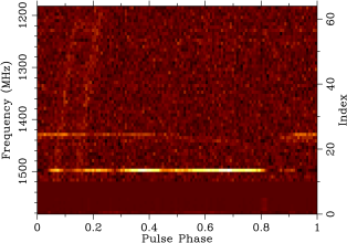
Figure 1: Narrow-band radio frequency interference that is not automatically detected by the default configuration of the zap median algorithm.

To understand why this seemingly-obvious RFI is not detected automatically, it is important to note that psrplot -p freq displays the pulsed flux as a function of pulse phase, whereas by default zap median works with the total flux summed over all pulse phases, which is plotted using

     psrplot -p psd example.ar     and is shown in the top panel of Figure 2.

Figure 2: Top panel: Spectrum formed by summing the values of all pulse phase bins for each frequency channel. Bottom panel: Pulsed spectrum formed by the difference between maximum and minimum values of all pulse phase bins for each frequency channel.

Here, the channels that have been corrupted by RFI are not as obvious. To utilize a statistic that better characterizes pulsed flux, note that both the psd plot and the zap median algorithm can be configured to use any expression that is understood by psrstat. For example,

     psrplot -p psd -c ’exp={$all:max-$all:min}’ example.ar     produces the pulsed flux spectrum shown in the bottom panel of Figure 2. The same expression can be used to configure the zap median algorithm, as in the following psrsh script

  zap.psh  #! /usr/bin/env psrsh# set the expression evaluated in each frequency channelzap median exp={$all:max-$all:min}# execute the zap median algorithmzap median# zap frequency channels 0 to 8zap chan 0-8 This script can be passed to psrplot and used to process the data before plotting.

     cd $PSRCHIVE_DATA/zap/BPSR  psrplot -p freq -J zap.psh example.ar     Alternatively, the script can be made executable and run like a psrchive program with the standard output option to write the result to a file with a new extension.

     chmod a+x zap.psh  ./zap.psh -e zz example.ar     

6.3 Automatic detection and removal of impulsive interference

Radio frequency interference (RFI) may also occur as broadband bursts of impulsive emission, such as lightning. When impulsive interference is persistent, it may not be possible to discard a subset of corrupted frequency channels or sub-integrations. To address this problem, psrchive implements an automatic impulsive interference mitigation algorithm that is based on tolerance to differences between the observed pulse profile and a version of the profile that has been smoothed by a running median. To detect impulsive RFI of terrestrial origin, the pulse profile is first integrated over all frequency channels without correcting for interstellar dispersion. The running median is then computed using a window with a duty cycle of 2% and any phase bin with total flux that differs from the median-smoothed profile by more than 4 times the standard deviation is flagged for replacement. By default, the standard deviation is defined recursively in a manner similar to the algorithm used for excising corrupted frequency channels. The default recursive standard deviation estimator will fail in extreme cases of impulsive RFI, and in general it is better to enable the use of robust statistics (e.g. the median absolute deviation) as demonstrated in the exercise below.

After flagging corrupted phase bins, the profiles in each frequency channel and polarization are corrected independently. A median-smoothed profile is computed and the values of flagged phase bins are set equal to the local median plus uncorrupted noise, defined as the difference between the observed profile and the local median of a randomly selected phase bin that has not been flagged as corrupted.

Exercise: Use psrplot and the zap mow pre-processing command to view an example of data corrupted by impulsive RFI that is not detected automatically by the default configuration of the algorithm.

     cd $PSRCHIVE_DATA/zap/DFB3  psrplot -p freq+ -jp -j "zap mow" -l subint=0- calibrator.ar     The above command will produce four separate plots, one for each sub-integration, the first of which is shown in Figure 3. To enable the use of robust statistics and increase the median smoothing duty cycle from 2% to 10%, create the following psrsh script

  mow.psh  #! /usr/bin/env psrsh# use robust statistics (median absolute deviation)zap mow robust# set the median-smoothing window to 10% of the pulse profilezap mow window=0.1# execute the zap mow algorithmzap mow and pass this script to psrplot to process the data before plotting.

     cd $PSRCHIVE_DATA/zap/DFB3  psrplot -p freq+ -jp -J mow.psh -l subint=0- calibrator.ar     The first plot produced by running the above command is shown in Figure 4.

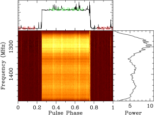
Figure 3: Impulsive radio frequency interference that is not automatically detected by the default configuration of the zap mow algorithm.

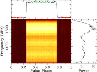
Figure 4: Impulsive radio frequency interference is detected by the zap mow algorithm after enabling the use of robust statistics and increasing the median smoothing duty cycle to 10%.

6.4 Interactive excision with psrzap

In some cases, automated methods of detecting corrupted data are insufficient and it is necessary to perform the task manually. Large data files with multiple sub-integrations and frequency channels are best visualized using a dynamic spectrum in which the colour of each pixel in a two-dimensional image spanned by time and frequency is determined by a value computed from the pulse profile at that coordinate. The psrzap program is an interactive tool for excising corrupted data using the dynamic spectrum. Run psrzap -h for a list of the keyboard and mouse interactive commands, then

     cd $PSRCHIVE_DATA/zap/GUPPI  psrzap guppi_55245_1909-3744_0033_0001.rf     After loading the data file, two plot windows will open. The main window plots the dynamic noise spectrum, which by default is defined as the variance in each pulse profile as a function of sub-integration (x-axis) and frequency (y-axis). The secondary plot window is divided into three panels: the top panel displays the pulse profile after integration over all time sub-integrations and frequency channels, the middle panel displays the phase-versus-frequency image after integration over all time sub-integrations, and the bottom panel displays the phase-versus-time image after integration over all frequency channels. These diagnostic plots are updated by pressing d on the keyboard.

As with psrplot -p psd and zap median, the quantity that is plotted as a function of time and frequency may be specified using a mathematical expression that is understood by psrstat; e.g.

     psrzap -E ’{$all:max-$all:min}’ guppi_55245_1909-3744_0033_0001.rf     There are three modes for selecting ranges of data to view or excise:

1. time (t on keyboard) selects an entire sub-integration (column)

2. frequency (f on keyboard) selects an entire frequency channel (row)

3. both (b on keyboard) selects a rectangular region

The line(s) passing through the cursor indicate the current selection mode. To zoom in on a desired range, click the left mouse button at the start and end positions of the range. To excise a desired range, click the left mouse button at the start, and the right mouse button at the end of the range. Simply right clicking will excise the single column, row, or pixel under the mouse (depending on the selection mode).

RFI typically appears as bright spots in the dynamic noise spectrum. Excise corrupted data until you are satisfied and save the result by pressing s on the keyboard. Press w to generate a psrsh command script that reproduces the results of the interactive excision session; the script is saved as a text file with a filename created by appending the .psh extension to the filename of the input archive. This script can be integrated into an automated pipeline that reprocesses the original data from scratch. Use psrstat to compare the $S/N$ of the data before and after RFI excision.

     psrstat -jTFp -c snr guppi_55245_1909-3744_0033_0001.rf*     

7 Polarimetric Calibration

Polarization measurements provide additional insight into the physics of both the emission and propagation of electromagnetic radiation; e.g. measurements of Faraday rotation in the interstellar medium yield constraints on the structure of the Galactic magnetic field (Han et al., 2006) and estimates of the position angle of the linearly polarized flux indicate that the pulsar spin axis may be aligned with its space velocity (Johnston et al., 2005). It has also been demonstrated that accurate polarimetry and arrival time estimation using all four Stokes parameters can signficantly improve both the accuracy and precision of pulsar timing data (van Straten, 2006).

The processes of reception and detection introduce instrumental artifacts that must be calibrated before meaningful interpretations of experimental data can be made. A first-order approximation to calibration can be performed using observations of a noise diode that is coupled to the receptors, from which the complex gains of the instrumental response as a function of frequency are derived. This approximation to calibration is based on the ideal feed assumption that the Jones matrix in each frequency channel has the form

$${\bf J}=\left(\begin{array}[]{cc}z_{0}&0\\ 0&z_{1}\end{array}\right)$$ (1)

where $z_{0}$ and $z_{1}$ are the complex gains. The absolute phase of the Jones matrix is lost during detection, and the matrix may be parameterized using a polar decomposition described by the absolute gain $G$, differential gain $\gamma$, and differential phase $\phi$.

7.1 Display calibrator parameters with psrplot

In psrchive, calibrator observations of the noise diode have type=PolnCal (as returned by psredit); the noise diode is typically driven by a square wave with a 50% duty cycle, as shown in Figures 3 and 4.

Exercise: Plot the polar decomposition of the ideal feed as a function of frequency.

     cd $PSRCHIVE_DATA/mem/cal  psrplot -p calm *.zz     

7.2 Prepare flux calibrator data with fluxcal

Although not immediately necessary for pulsar timing, it is also useful to perform absolute flux calibration; for example, well-calibrated estimates of flux density may be used in long-term studies of refractive scintillation (e.g. Rickett et al., 1984). Absolute flux calibration is performed using observations of a standard candle, an astronomical source with a well-determined reference flux density and spectral index that applies over a broad range of radio frequencies. Two sets of observations are made: the noise diode is driven while the telescope is pointed at 1) the standard candle and 2) a nearby patch of sky that is assumed to be empty. Example plots derived from the sample data are shown in Figure 5.

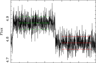
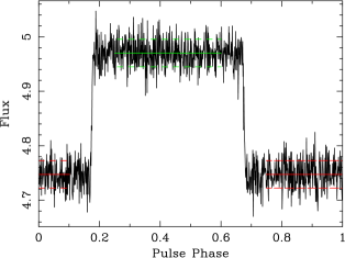
Figure 5: Observations of the Parkes 21-cm Multibeam receiver noise source. The total intensity from a single 500 kHz channel was integrated for approximately 80 s. In the top panel, the telescope was pointed at 3C 218 (Hydra A); the mean on-pulse power (green) is used to estimate $H_{\rm on}$ and the mean off-pulse power (red) is used to estimate $L_{\rm on}$. In the bottom panel, the telescope was pointed 2 deg north; the mean on-pulse power is used to estimate $H_{\rm off}$ and the mean off-pulse power is used to estimate $L_{\rm off}$.

Note that the integration lengths for the on- and off-source observations need not necessarily be equal (as long as the data represent mean flux densities). The absolute gains also need not be equal. Given

$H_{\rm on}=g_{\rm on}(S_{\rm sys}+T_{0}+C_{0})$	$H_{\rm off}=g_{\rm off}(S_{\rm sys}+C_{0})$
$L_{\rm on}=g_{\rm on}(S_{\rm sys}+T_{0})$	$L_{\rm off}=g_{\rm off}S_{\rm sys}$

where $g_{\rm on}$ and $g_{\rm off}$ are the unknown absolute gains of the instrument while pointing on and off the standard candle, $S_{\rm sys}$ is the unknown system equivalent flux density, $S_{0}$ is the known flux density of the standard candle, and $C_{0}$ is the unknown flux density of the receiver noise source. Then,

$$f_{\rm on}={H_{\rm on}\over L_{\rm on}}-1={C_{0}\over S_{\rm sys}+S_{0}}$$ (2)

and

$$f_{\rm off}={H_{\rm off}\over L_{\rm off}}-1={C_{0}\over S_{\rm sys}}$$ (3)

and

$${1\over f_{\rm on}}-{1\over f_{\rm off}}={S_{0}\over C_{0}}$$ (4)

Equation 4 is solved for $C_{0}$, then Equation 3 is solved for $S_{\rm sys}$. In psrchive, flux calibration observations have a type attribute equal to FluxCalOn or FluxCalOff.

Exercise: Start by creating a calibrator database.

     cd $PSRCHIVE_DATA/mem/cal  pac -w -u zz     This creates a file called database.txt. Then run

     fluxcal -f -d database.txt     This will produce a file named n2003201035947.fluxcal and update database.txt with a new entry for this file. Use psrplot -p calm to plot the derived estimates of $S_{\rm sys}$ and $S_{0}$ as a function of radio frequency).

7.3 Correct the receiver parameters

A large number of assumptions are built into the design of an instrument, ranging from the sign of the complex argument in $\exp(\pm i\omega t)$ to the handedness of circular polarization. Over time, a number of inconsitent conventions have been utilised by various authors; e.g. see Everett & Weisberg (2001) for a thorough review of contradicting definitions of the position angle of the linearly polarized flux.

To address this issue, van Straten et al. (2010) define the PSR/IEEE convention that is used by psrchive and include a table of parameters that can be used to describe the differences between an instrumental design and the PSR/IEEE convention. For the Parkes 21-cm Multibeam receiver, it is necessary to set the symmetry angle to $-\pi/2$, which can be done with the following command

     cd $PSRCHIVE_DATA/mem  psredit -c rcvr:sa=-90 -m pulsar/*.ar cal/*.ar     

7.4 Calibrate using the ideal feed assumption

To perform the first-order approximation to calibration based on the ideal feed assumption, run

     cd $PSRCHIVE_DATA/mem/pulsar  pac -d ../cal/database.txt *.zz     For each input file, a new output file will be written with a filename created by appending the extension .calib to the input filename. If the receiver were ideal, the first-order approximation to calibration would have eliminated the variation of the Stokes parameters as a function of parallactic angle. Use psrplot to test this expectation.

     psrplot -ps -jF *.calib     The Stokes parameters still vary as a function of time because the ideal feed assumption does not apply to the Parkes 21-cm Multibeam receiver. Create a sub-directory, e.g. ideal/ and move the newly calibrated data to this sub-directory (otherwise, they will be over-written in the next step).

     mkdir ideal  mv *.calib ideal/     

7.5 Measure the cross-coupling parameters using pcm

To accurately calibrate these data, the cross-coupling terms (off-diagonal components of the Jones matrix) must be estimated, which can be done by modeling the variation of the Stokes parameters as a function of time. The process of performing the least-squares fit is called Measurement Equation Modeling (MEM); the psrchive implementation is described in van Straten (2004) and more fully documented online. Use psradd to combine the archives calibrated using the ideal feed assumption into a single archive

     psradd -T -o calib.TT ideal/*.calib     The resulting archive will be used as input to pcm, from which it will choose the best phase bins to use as constraints and derive the first guess for the polarization of the source.

     pcm -d ../cal/database.txt -s -c calib.TT *.zz     While running, pcm outputs messages about the quality of the least-squares fits, which are performed independently in each frequency channel. On a multi-processor machine, multiple channels may be solved simultaneously by using the -t <nthread> command-line option, where <nthread> is the number of processing threads to run in parallel. When pcm finishes, it produces an output file pcm.fits that contains the MEM solution; the model parameters may be plotted using

     psrplot -p calm pcm.fits     Compared to the solution derived using the ideal feed assumption, three new parameters have been added to the model of the receiver: $\theta_{1}$ describes the non-orthogonality of the feed receptors (the linearly polarized receptors should be oriented at 0 and 90 degrees) and $\epsilon_{k}$ are the ellipticities of the receptors, which should be 0 in an ideal feed with linearly polarized receptors. The mean value of $\sim 5$ degrees corresponds to roughly 15% mixing between linear and circular polarizations (Stokes $Q$ and $V$). It is not possible to determine the absolute rotation of the receptors about the line of sight, $\theta_{0}$, without an external reference; therefore, only the non-orthogonality is measured.

The solution output by pcm also includes estimates of the Stokes parameters of the noise diode, which is no longer assumed to illuminate both receptors equally and in phase. This information enables the calibrator solution derived from one data set to be applied to observations of another source, as in Ord et al. (2004).

7.6 Calibrate using the MEM solution

Move the output file pcm.fits to the cal/ sub-directory, change to this directory, and recreate the calibrator database

     mv pcm.fits ../cal/  cd ../cal  pac -w -u zz -u fits -u fluxcal     Confirm that pcm.fits has been added to database.txt, then run

     cd ../pulsar  pac -d ../cal/database.txt -S *.zz     Plot the Stokes polarization profile (integrated over the entire band) in each calibrated data file output by pac to confirm that the Stokes parameters no longer vary with time.

8 Arrival time estimation

In this section, arrival time estimates are derived using a previously created standard (template) profile. This high $S/N$ standard profile was formed by integrating data from $\sim 42$ hours of observations.

8.1 Prepare the standard profile

The standard profile is located in $PSRCHIVE_DATA/mem/std/standard.ar. Plot the phase-vs-frequency image of the total intensity and compare this image with that of nonspc.ar in the same directory. The file nonspc.ar was formed from data that were not corrected for scattered power. Although standard.ar was corrected, there are still residual artefacts in the edges of the band. Use psrsh to give zero weight to the affected frequency channels then integrate over all frequency channels. For best results, excise the same frequency channels that were excised from the data in Section 6.1; e.g.

     cd $PSRCHIVE_DATA/mem/std  psrsh - -e FF standard.ar << EOD  zap edge 0.15  fscrunch  EOD     If the GNU Scientific Library is installed and detected during the configuration of the psrchive software, then it is possible to use the wavelet smoothing algorithm implemented by psrsmooth to create a “noise-free” template profile.

     psrsmooth -W -t UD8 standard.FF     This will produce a file called standard.FF.sm. By default, psrsmooth applies the translation-invariant wavelet denoising algorithm described by Coifman & Donoho (1995). The profile data are first transformed into the wavelet domain, where a noise level is estimated from the data. Based on the measured noise level, a threshold is calculated, and all wavelet coefficients with absolute value below the threshold level are set to zero. The data are then transformed back into the profile domain, resulting in a smoothed profile. Use the crop attribute of the flux plot to zoom in on the low amplitude flux near the off-pulse baseline and compare the standard profile with its smoothed version; e.g.

     psrplot -pD -jp -c crop=0.01 -N 1x2 standard.FF standard.FF.sm     

8.2 Estimate arrival times using pat

In this section, two different methods of arrival time estimation are compared: scalar template matching using only the total intensity (Taylor, 1992) and matrix template matching using all four Stokes parameters (van Straten, 2006). Comparison is also made between the results derived using the two different template profiles: the smoothed and not smoothed versions of standard.ar. Finally, there are three different data sets: the uncalibrated data, the data calibrated using the ideal feed assumption, and the data calibrated using the MEM solution derived with pcm. In total, there are 12 different combinations of arrival time estimation algorithm, template profile, and observational data. Experiment with these combinations to find the arrival times with the lowest residual standard deviation. To experiment, run pat in either scalar template matching mode; e.g.

     cd $PSRCHIVE_DATA/mem/pulsar  pat -F -s ../std/standard.FF *.zz > uncal_unsmooth_stm.tim     or matrix template matching mode; e.g.

     pat -Fpc -s ../std/standard.FF.sm *.calib > cal_smooth_mtm.tim     Run tempo2 to evaluate the arrival times; e.g.

     tempo2 -f ../pulsar.par uncal_unsmooth_stm.tim     Search the output of tempo2 for lines like

     RMS pre-fit residual = 0.11 (us), RMS post-fit residual = 0.11 (us)  Fit Chisq = 359.7       Chisqr/nfree = 359.74/95 = 3.78671     and make note of both the RMS post-fit residual and Chisqr/nfree in each case tested.

8.3 Correct arrival time estimation bias using psrpca

As the mean flux density of a source of noise approaches the system equivalent flux density, the statistics of the noise intrinsic to the source (or self-noise) can no longer be neglected (e.g. Gwinn, 2001; van Straten, 2009; Gwinn & Johnson, 2011). This is particularly true when the signal is heavily modulated, as is typically the case with pulsar emission (Rickett, 1975), which can be described as stochastic wide-band impulse modulated self-noise (SWIMS; Osłowski et al., 2011). Pulsed self-noise is heteroscedastic and, when the timescale of impulsive modulation is longer than the sampling interval required to resolve the mean pulse profile, SWIMS is correlated. Correlated and heteroscedastic noise violates the basic premises of least-squares estimation and introduces pulse arrival time measurement bias. This bias may be corrected using psrpca, which performs a principle component analysis of the observed pulse profile shape fluctuations and a multiple regression analysis in which the post-fit arrival time residual is the dependent variable and the most significant principal components are the independent variables. The methodology is described in detail by Demorest (2007) and Osłowski et al. (2011).

SWIMS is best characterised using a large quantity of data; at the very least, the number of observations must exceed the number of phase bins used to resolve the mean pulse profile. This constraint is satisfied by the example data: $\sim$ 9000 pulse profiles spanning $\sim 10$ days of observations of PSR J0437$-$4715 made at 20 cm with the Parkes 64 m radio telescope between 19 and 27 July 2003. To measure and remove the arrival time bias introduced by SWIMS, first produce the arrival time estimates

     cd $PSRCHIVE_DATA/pca  ls -1 *.ar > files.ls  pat -s ../mem/std/standard.FF -f tempo2 -M files.ls > psrpca.tim     then compute the post-fit arrival time residuals

     tempo2 -output general2  -s ’{sat} {post} {err} SWIMS\n’ \  -f ../mem/pulsar.par psrpca.tim | grep SWIMS \  | awk ’{print $1,$2,$3}’ > resid.dat     and perform the principal component and multiple regression analyses

     psrpca -s ../mem/std/stanard.FF -r resid.dat -M files.ls     When running psrpca, it is important to ensure that the arrival time residuals and input data files are provided in exactly the same order. The above commands ensure this by first creating a file listing named files.ls, which is passed to both pat and psrpca. A variety of diagnostic output files are produced by psrpca, each with a name that starts with the prefix psrpca; this prefix can be chosen by using the -p prefix option. The diagnostic output files are:

• psrpca_diffs.ar – an archive containing the differences between the standard template and observed pulse profiles; these data are used to construct the covariance matrix;

• psrpca_covariance.dat – a plain text file containing the covariance matrix;

• psrpca_evals.dat – a plain text file containing the eigenvalues derived from the covariance matrix in a format that is easily inspected using gnuplot;

• psrpca_evecs.ar – a psrfits archive containing the eigenvectors;

• psrpca_decomposition.dat – a plain text file containing the decompositions of the observed pulse profiles onto the measured eigenvectors;

• psrpca_beta_zero.dat and psrpca_beta_vector_used.dat – plain text files containing the regression coefficients used to remove the bias in arrival time estimates; and

• psrpca_residuals.dat – a plain text file containing the bias-corrected arrival time residuals.

These output files enable easy inspection of the principal component analysis results. The plain-text output file named psrpca_residuals.dat contains four columns:

1. MJD – the site arrival time;

2. biased_residual – the arrival time residual produced by tempo2 (expressed in $\mu s$)

3. corrected_residual – the bias-corrected arrival time residual

4. error – the estimated measurement error produced by pat

This file can be used to compare the biased and corrected arrival time residuals. The provided script rms.sh may be used to compare the standard deviation of the two sets of arrival time residuals; e.g.

     ./rms.sh psrpca_residuals.dat 2 4  ./rms.sh psrpca_residuals.dat 3 4     The first command produces the weighted standard deviation and a measure of goodness of fit for the biased arrival time residuals; the latter computes the same for the bias-corrected residuals. The biased and corrected residuals may also be inspected using gnuplot.

The primary output of the psrpca program is a file named psrpca_std.ar. This psrfits archive contains a copy of the standard template profile that was provided to psrpca with an additional extension that contains the principal component eigenvectors and the multiple regression coefficients. pat can use the information in this extension to correct the bias in output arrival time estimates. With this functionality, the bias predictor derived from one epoch may be applied to observations made at other epochs and the bias-corrected arrival time estimates may be provided as input to tempo or tempo2, thereby yielding improved physical parameter estimates.

9 Discussion

This paper presents a scientific workflow for high-precision timing experiments and demonstrates some of the general-purpose tools applicable to a wider variety of pulsar studies. In addition to the programs described here, psrchive development continues on a number of novel analysis tools.

For example, the psrmodel program fits the rotating vector model (Radhakrishnan & Cooke, 1969; Everett & Weisberg, 2001) to observed polarisation data using a statistically robust algorithm. Rather than perform a one-dimensional fit to the real-valued position angle as a function of pulse phase, psrmodel performs a two-dimensional fit directly to the Stokes $Q$ and Stokes $U$ profiles by treating them as the real and imaginary components of a complex number. For each complex number, the phase is given by the position angle predicted by the rotating vector model and the magnitude (linearly polarized flux) is modeled as a free parameter. This approach has a number of advantages over directly modeling the position angle: 1) because Stokes $Q$ and $U$ errors are normally distributed, low $S/N$ data may be included in the fit without biasing the result; 2) Stokes $Q$ and $U$ are not cyclic; and 3) orthogonal mode transitions are trivially modeled by negative values of the complex magnitudes.

Also currently under development, the psrspa program can search for significant single pulses and derive a wide variety of statistical quantities from single-pulse data, such as the phase-resolved histogram of the position angle (e.g. Stinebring et al., 1984) and the two-dimensional distribution of the polarization vector orientation (Edwards & Stappers, 2004; McKinnon, 2009). This program was recently used to analyse the phase distribution and width of single pulses from the radio magnetar, PSR J1622$-$4950 (Levin et al., 2012).

A number of the algorithms implemented by psrchive consist of a single, independent profile transformation that is performed sequentially by looping over all sub-integrations and frequency channels. On a multiprocessor architecture, such transformations could be readily executed in parallel; furthermore, identification of such parallelism also provides the opportunity to apply loop transformations that improve data locality and conserve memory bandwidth (e.g. Abu-Sufah, 1979; McKinley et al., 1996).

Though written in C++, it is possible to access a large fraction of psrchive functionality via the Python programming language. This provides an alternative to the psrchive applications and psrsh command language interpeter for both high-level scripting of psrchive functionality and interactive or non-standard data manipulation. The Python interface works by providing direct access to the core C++ class library on which psrchive is built. Additional information about installing and using the Python interface is available in the online documentation. Developers with an interest in extending, refining, or optimising the psrchive software are encouraged to contact the project administrators and refer to the extensive online documentation hosted by sourceforge.

Acknowledgements The authors are grateful to Cees Bassa, Aidan Hotan, Andrew Jameson, Mike Keith, Jonathan Khoo and Aris Noutsos for valuable contributions to the psrchive software. We also thank Han JinLin and his students and colleagues for technical assistance with the preparation of this manuscript, including translation of the title and abstract.

Appendix A Obtaining data from the CSIRO Data Access Portal

To obtain a copy of the observational data used in this paper, visit the CSIRO Data Access Portal and, using the Pulsar Search tool, enter the following information

• Source Name: J0437-4715

• Project ID: P140

• Observation Date (dd/mm/yyyy): 19/07/2003 to 27/07/2003

Using the check boxes in the column on the left, refine the search results to include only “raw” observations (i.e. not preprocessed) with a frequency of 1341 MHz. This should yield 67 results, the first of which has the filename n2003-07-19-18:08:01.rf, and a total download size of 15.3 GB.

The data stored on the CSIRO Data Access Portal have more time and frequency resolution than is required for the purposes of the demonstrations presented in this paper. Processed versions of these data with lower resolution are also available for download from Swinburne University of Technology at

http://astronomy.swin.edu.au/pulsar/data

Here, there are three files

• psrchive_mem.tgz (112.6 MB) contains 5-minute integrations with full frequency resolution from the first day of observations (19 July 2003) – these data are for use in the exercises presented in Sections 2 through 8;

• psrchive_zap.tgz (299.4 MB) contains three files that are not available via the CSIRO Data Access Portal – these data are for use in the exercises presented in Section 6; and

• psrchive_pca.tgz (132.4 MB) contains $\sim 17$-second integrations with no frequency resolution spanning the nine days of observations (from 19 to 27 July 2003) – these data are for use in the exercises presented in Section 8.3

These files can be unpacked with commands such as

     gunzip -c psrchive_mem.tgz | tar xf -     The examples presented throughout this paper assume that the above three files have been downloaded from Swinburne University of Technology and the full path to the directory into which they have been unpacked is recorded using the $PSRCHIVE_DATA shell environment variable.

References

- Abu-Sufah (1979) Abu-Sufah, W. A.-K. 1979, Improving the performance of virtual memory computers., Ph.D. thesis, Champaign, IL, USA
- Coifman & Donoho (1995) Coifman, R. R., & Donoho, D. L. 1995, in Wavelets and Statistics, Springer Lecture Notes in Statistics, vol. 103, 125–150
- Demorest (2007) Demorest, P. B. 2007, Measuring the Gravitational Wave Background using Precision Pulsar Timing, Ph.D. thesis, University of California, Berkeley
- Demorest (2011) Demorest, P. B. 2011, MNRAS, 416, 2821
- Edwards et al. (2006) Edwards, R. T., Hobbs, G. B., & Manchester, R. N. 2006, MNRAS, 372, 1549
- Edwards & Stappers (2004) Edwards, R. T., & Stappers, B. W. 2004, A&A, 421, 681
- Everett & Weisberg (2001) Everett, J. E., & Weisberg, J. M. 2001, ApJ, 553, 341
- Gwinn (2001) Gwinn, C. R. 2001, ApJ, 561, 815
- Gwinn & Johnson (2011) Gwinn, C. R., & Johnson, M. D. 2011, ApJ, 733, 51
- Han et al. (2006) Han, J. L., Manchester, R. N., Lyne, A. G., Qiao, G. J., & van Straten, W. 2006, ApJ, 642, 868
- Hanisch et al. (2001) Hanisch, R. J., Farris, A., Greisen, E. W., et al. 2001, A&A, 376, 359
- Hotan et al. (2005) Hotan, A. W., Bailes, M., & Ord, S. M. 2005, ApJ, 624, 906
- Hotan et al. (2004) Hotan, A. W., van Straten, W., & Manchester, R. N. 2004, PASA, 21, 302
- Jenet et al. (1998) Jenet, F., Anderson, S., Kaspi, V., Prince, T., & Unwin, S. 1998, ApJ, 498, 365
- Johnston et al. (2005) Johnston, S., Hobbs, G., Vigeland, S., et al. 2005, MNRAS, 364, 1397
- Johnston et al. (1993) Johnston, S., Lorimer, D. R., Harrison, P. A., et al. 1993, Nature, 361, 613
- Kramer et al. (1998) Kramer, M., Xilouris, K. M., Lorimer, D. R., et al. 1998, ApJ, 501, 270
- Levin et al. (2012) Levin, L., Bailes, M., Bates, S. D., et al. 2012, MNRAS, 2751
- Lorimer (2001) Lorimer, D. R. 2001, SIGPROC-v1.0: (Pulsar) Signal Processing Programs, Arecibo Technical Memo No. 2001–01
- Lorimer et al. (1998) Lorimer, D. R., Jessner, A., Seiradakis, J. H., et al. 1998, A&AS, 128, 541
- Manchester et al. (2005) Manchester, R. N., Hobbs, G. B., Teoh, A., & Hobbs, M. 2005, AJ, 129, 1993
- Manchester et al. (1996) Manchester, R. N., Lyne, A. G., D’Amico, N., et al. 1996, MNRAS, 279, 1235
- McKinley et al. (1996) McKinley, K. S., Carr, S., & Tseng, C.-W. 1996, ACM Trans. Program. Lang. Syst., 18, 424
- McKinnon (2009) McKinnon, M. M. 2009, ApJ, 692, 459
- Navarro et al. (1997) Navarro, J., Manchester, R. N., Sandhu, J. S., Kulkarni, S. R., & Bailes, M. 1997, ApJ, 486, 1019
- Noutsos et al. (2008) Noutsos, A., Johnston, S., Kramer, M., & Karastergiou, A. 2008, MNRAS, 386, 1881
- Ord et al. (2004) Ord, S. M., van Straten, W., Hotan, A. W., & Bailes, M. 2004, MNRAS, 352, 804
- Osłowski et al. (2011) Osłowski, S., van Straten, W., Hobbs, G. B., Bailes, M., & Demorest, P. 2011, MNRAS, 418, 1258
- Radhakrishnan & Cooke (1969) Radhakrishnan, V., & Cooke, D. J. 1969, Astrophys. Lett., 3, 225
- Ransom et al. (2003) Ransom, S. M., Cordes, J. M., & Eikenberry, S. S. 2003, ApJ, 589, 911
- Ransom et al. (2002) Ransom, S. M., Eikenberry, S. S., & Middleditch, J. 2002, AJ, 124, 1788
- Rickett (1975) Rickett, B. J. 1975, ApJ, 197, 185
- Rickett et al. (1984) Rickett, B. J., Coles, W. A., & Bourgois, G. 1984, A&A, 134, 390
- Sandhu et al. (1997) Sandhu, J. S., Bailes, M., Manchester, R. N., et al. 1997, ApJ, 478, L95
- Stinebring et al. (1984) Stinebring, D. R., Cordes, J. M., Rankin, J. M., Weisberg, J. M., & Boriakoff, V. 1984, ApJS, 55, 247
- Taylor (1992) Taylor, J. H. 1992, Philos. Trans. Roy. Soc. London A, 341, 117
- Taylor & Weisberg (1989) Taylor, J. H., & Weisberg, J. M. 1989, ApJ, 345, 434
- van Straten (2004) van Straten, W. 2004, ApJS, 152, 129
- van Straten (2006) van Straten, W. 2006, ApJ, 642, 1004
- van Straten (2009) van Straten, W. 2009, ApJ, 694, 1413
- van Straten & Bailes (2011) van Straten, W., & Bailes, M. 2011, PASA, 28, 1
- van Straten et al. (2010) van Straten, W., Manchester, R. N., Johnston, S., & Reynolds, J. E. 2010, PASA, 27, 104