Large-sample study of the kernel density estimators under multiplicative censoring

Abstract

The multiplicative censoring model introduced in Vardi [Biometrika 76 (1989) 751–761] is an incomplete data problem whereby two independent samples from the lifetime distribution $G$, $\mathcal{X}_{m}=(X_{1},\ldots,X_{m})$ and $\mathcal{Z}_{n}=(Z_{1},\ldots,Z_{n})$, are observed subject to a form of coarsening. Specifically, sample $\mathcal{X}_{m}$ is fully observed while $\mathcal{Y}_{n}=(Y_{1},\ldots,Y_{n})$ is observed instead of $\mathcal{Z}_{n}$, where $Y_{i}=U_{i}Z_{i}$ and $(U_{1},\ldots,U_{n})$ is an independent sample from the standard uniform distribution. Vardi [Biometrika 76 (1989) 751–761] showed that this model unifies several important statistical problems, such as the deconvolution of an exponential random variable, estimation under a decreasing density constraint and an estimation problem in renewal processes. In this paper, we establish the large-sample properties of kernel density estimators under the multiplicative censoring model. We first construct a strong approximation for the process $\sqrt{k}(\hat{G}-G)$, where $\hat{G}$ is a solution of the nonparametric score equation based on $(\mathcal{X}_{m},\mathcal{Y}_{n})$, and $k=m+n$ is the total sample size. Using this strong approximation and a result on the global modulus of continuity, we establish conditions for the strong uniform consistency of kernel density estimators. We also make use of this strong approximation to study the weak convergence and integrated squared error properties of these estimators. We conclude by extending our results to the setting of length-biased sampling.

abstractwidth280pt

, and

T3Authorship is listed alphabetically to reflect the equal contribution of each author.

t1Supported in part by NSERC, FQRNT and the Veterans Affairs HSR&D Service.

t2Supported in part by NSERC, FQRNT, NIH and the Hopkins Sommer Scholars Program.

1 Introduction

Vardi vardi1989biometrika introduced an incomplete data problem unifying several statistical models. The problem consisted of inferring the lifetime distribution of interest $G$ through a random sample $X_{1},X_{2},\ldots,X_{m}$ drawn directly from $G$ and a random sample $Y_{1},Y_{2},\ldots,Y_{n}$ drawn from the distribution $F$ with density function

$$f(y)=\int_{y\leq z}z^{-1}\,dG(z),\qquad y>0.$$ (1)

Since $f$ is a decreasing density function, $Y$ may be expressed as the product of two independent random variables: a nonnegative variate $Z$ and a standard uniform variate $U$. From the form of (1), it is easy to see that in this case $Z$ must be distributed according to $G$. This representation suggests that only a random fraction of $Z$ may be observed, motivating the nomenclature multiplicative censoring used to describe this incomplete data scheme. The likelihood based on the $k=m+n$ observations $X_{1}=x_{1},\ldots,X_{m}=x_{m}$ and $Y_{1}=y_{1},\ldots,Y_{n}=y_{n}$ is

$$L(G)=\prod_{i=1}^{m}G(dx_{i})\prod_{j=1}^{n}\int_{y_{j}\leq z}z^{-1}\,dG(z).$$ (2)

As discussed by Vardi vardi1989biometrika , the multiplicative censoring model arises from the deconvolution of an exponential random variable, estimation under a decreasing density constraint and an estimation problem in renewal processes. The literature on these and related problems is vast. Estimation under a decreasing density constraint dates back to the seminal work of Grenander grenander1956actscand , with key contributions by Groeneboom groeneboom1985berkconf and Huang and Wellner huang1995scand . The estimation problem in renewal processes discussed in vardi1989biometrika is closely tied to important applications in cross-sectional sampling and prevalent cohort studies in epidemiology (length-biased sampling) and in labor force studies in economics (stock sampling). The multiplicative censoring model and its variants have been studied by hasminskii1983ln , vardi1989biometrika , bickel1994theoryprob , bickel1993 , vandervaart1994annals and vardi1992lannals , among others. Vardi vardi1992lannals studied the asymptotic behavior of solutions of the nonparametric score equation under the multiplicative censoring model.

As will be discussed later, multiplicative censoring and left-truncated right-censored data are intricately tied. The latter have been extensively studied in the statistical literature. Their importance stems mainly, although not exclusively, from the widespread use of prevalent cohort study designs to estimate survival from onset of a disease. In such studies, patients with prevalent disease are identified at some instant in calendar time, often through a cross-sectional survey. These patients are then followed forward in time until death or loss to follow-up. If no temporal change in the incidence of disease has occurred during the period covering observed onsets, a stationary Poisson process may adequately describe the incidence pattern of the disease; see asgharian2006statsinmed , asgharian2002jasa , asgharian2005annals and wolfson2001nejm . In this case, the left-truncation variable is uniformly distributed, and the failure time data are said to be length-biased. The likelihood for the observed data is then given by (2), where

$$G(t)=\mu_{U}^{-1}\int_{0}^{t}{u}\,dF_{U}(u),$$

$\mu_{U}=\int_{0}^{\infty}{u}\,dF_{U}(u)$ and $F_{U}$, the unbiased distribution, is the underlying distribution function about which we would like to infer; see Section 6 and asgharian2005annals . Because we require $\mu_{U}<\infty$ in the above, we restrict our attention to distribution functions $G$ such that $\int{z^{-1}\,dG(z)}<\infty$.

The connection between the multiplicative censoring model and prevalent cohort studies under the stationarity assumption has revived interest in the former. Nonetheless, there appears to be no result in the literature on density estimation under the multiplicative censoring model, despite its importance in applied sciences. A recent application described by Kvam kvam2008tech concerns nanoscience and the measurement of carbon nanotubes. As discussed by Silverman silverman1986 , density estimation can be useful for purposes of data exploration and presentation. It is effective in the investigation of modes (determination of multimodality and identification of modes) and tail behavior (rate of tail decay). These features are especially important in length-biased sampling and survival analysis, where skewness is often pervasive and differential subgroup characteristics may lead to multimodality. An additional motivation for the study of density estimation under multiplicative censoring stems from the fact that nonparametric regression of right-censored length-biased data has not been addressed in the literature. In view of the intricate link between density estimation and nonparametric regression (see nussbaum1996annals ), a study of density estimation under multiplicative censoring provides foundations for studying nonparametric regression of right-censored length-biased data.

Among the various methods of density estimation, kernel smoothing is particularly appealing for both its simplicity and its interpretability (e.g., as a limiting pointwise average of shifted histograms). It provides a unifying framework in that, as discussed in scott1992 , each of finite difference density estimation, smoothing by convolution, orthogonal series approximations and other smoothing methods historically used in the various applied sciences can be seen as instances of kernel smoothing. This article studies the large-sample properties of kernel density estimators in the setting of multiplicative censoring. Pioneered by Silverman silverman1978annals , the approach adopted consists of constructing strong approximations of the empirical density process.

Although under the multiplicative censoring model we may avoid complexities altogether by performing estimation using the uncensored observations alone, use of the full data is motivated by at least two reasons. First, although discarding the censored cases under the canonical multiplicative censoring scheme does not compromise consistency, the same cannot be said under the related length-biased sampling scheme, even though these schemes lead to the same likelihood. This occurs because, under length-bias sampling, the uncensored cases do not emanate directly from the (length-biased version of the) distribution of interest. Systematic exclusion of the censored cases would therefore lead to inconsistency. This fact motivates the study of both censored and uncensored cases under multiplicative censoring. Second, due to the informativeness of the censoring mechanism, ignoring the censored observations may lead to a substantial loss of efficiency. Because the asymptotic covariance function of the nonparametric maximum likelihood estimator of $G$ does not have an explicit form, this phenomenon is difficult to quantify in the nonparametric setting (see the discussion on page 1024 of vardi1992lannals ); however, a parametric example may be illustrative. Suppose that the uncensored observations emanate from a Gamma distribution, say with mean 2$\theta$ and variance $2\theta^{2}$, then the censored observations are exponentially distributed with mean $\theta$. The asymptotic relative efficiency of the full-sample MLE relative to the uncensored-sample MLE is $1+\upsilon/2$, where $\upsilon>0$ is the asymptotic relative frequency of censored observations to uncensored observations. If, for example, $\upsilon=1$, indicating that uncensored and censored cases arise in equal numbers asymptotically, use of the full sample provides a fifty percent gain in efficiency.

Following komlos1975zwvg , hereafter referred to as KMT, and csorgo1981 , we first construct a strong approximation for the process $\sqrt{k}(\hat{G}-G)$, where $\hat{G}$ is a solution of the nonparametric score equation based on $(\mathcal{X}_{m},\mathcal{Y}_{n})$. The literature on strong approximations is vast. Recent reviews on empirical processes, strong approximations and the KMT construction include delbarrio2007 and mason2007jspi . Using this strong approximation and a result on the global modulus of continuity, we obtain the strong uniform consistency of the kernel density estimators of the density function $g$ associated to $G$ and find a sequence of Gaussian processes strongly uniformly approximating the empirical kernel density process. Using these results, we study the integrated squared error properties of the kernel density estimators.

The layout of the paper is as follows. In Section 2, we introduce our notation and present some preliminaries. In Section 3, we find a sequence of Gaussian processes that strongly uniformly approximates the empirical process $\sqrt{k}(\hat{G}-G)$ and study its global modulus of continuity. We use these results to study the asymptotic behavior of the kernel density estimators in Section 4. It is shown, in particular, that the kernel density estimators are strongly consistent and asymptotically Gaussian. Section 5 is devoted to the integrated squared error properties of the kernel density estimators and includes results from a preliminary small-sample simulation study. We show how our results can be extended to length-biased sampling with right-censoring in Section 6 and present concluding remarks in Section 7. The claim and theorems are proved in the Appendix while lemmas are proved in the supplementary material asgharian2012supp .

2 Preliminaries

We consider the random multiplicative censoring model introduced in vardi1989biometrika , whereby two independent random samples $\mathcal{X}_{m}=(X_{1},\ldots,\allowbreak X_{m})$ and $\mathcal{Z}_{n}=(Z_{1},\ldots,Z_{n})$ are drawn from the lifetime distribution $G$ and a third independent sample $\mathcal{U}_{n}=(U_{1},\ldots,U_{n})$, from the standard uniform distribution. Let $Y_{i}=Z_{i}U_{i}$, $i=1,\ldots,n$, and write $\mathcal{Y}_{n}=(Y_{1},\ldots,Y_{n})$. Then $\mathcal{Y}_{n}$ is a random sample from the absolutely continuous distribution $F$ with density given by (1). The observed data consist of $(\mathcal{X}_{m},\mathcal{Y}_{n})$ while $(\mathcal{Z}_{n},\mathcal{U}_{n})$ is unobserved.

We begin with the score equation derived from the likelihood $L(G)$ given by (2). Let $G_{m}$ and $F_{n}$ be, respectively, the empirical distribution functions based on the uncensored observations $x_{1},\ldots,x_{m}$ and the censored cases $y_{1},\ldots,y_{n}$, and write $\hat{p}=m/k$, where $k=m+n$. For simplicity, assume all observations are distinct, and denote by $t_{1}<\cdots<t_{k}$ the values taken by $x_{1},\ldots,x_{m}$ and $y_{1},\ldots,y_{n}$. The distribution function $\hat{G}$ satisfies the nonparametric score equation if, for all $t\geq 0$,

$$d\hat{G}(t)=\hat{p}\,dG_{m}(t)+(1-\hat{p})\biggl{[}\int_{0<y\leq t}\frac{dF_{n}(y)}{\int_{y\leq z}z^{-1}\,d\hat{G}(z)}\biggr{]}t^{-1}\,d\hat{G}(t),$$ (3)

while $\sum_{j=1}^{k}d\hat{G}(t_{j})=1$ and $d\hat{G}(t_{j})\geq 0$, $j=1,\ldots,k$; see vardi1992lannals , page 1025. Integrating both sides of (3), we obtain

$$\hat{G}(t)=\hat{p}G_{m}(t)+(1-\hat{p})\int_{0<x\leq t}\biggl{[}\int_{0<y\leq x}\frac{dF_{n}(y)}{\int_{y\leq z}z^{-1}d\hat{G}(z)}\biggr{]}x^{-1}\,d\hat{G}(x),$$

where the final integrand is defined to be 0 for $x>t_{k}$. We say that a sequence of real numbers $\gamma_{m,n}$ satisfies assumption (A0) if

$$\sum_{m,n}G(\gamma_{m,n})<\infty,$$

where the summation is understood to range over subsample sizes $m$ and $n$, jointly taken to infinity, so that $\hat{p}\rightarrow p\in(0,1]$. To circumvent problems related to a singularity at the origin, we select a sequence of positive real numbers $\gamma_{m,n}$ satisfying (A0) and consider solutions $\hat{G}$ of (3) assigning zero mass below $\gamma_{m,n}$. All results derived in this article apply to any solution of (3) with this property. The existence of such solutions is an important fact.

Claim 1.

Suppose that (A0) holds. Then, for each $m$ and $n$ sufficiently large, (3) has a solution $\hat{G}$ such that $\hat{G}(u)=0$ for each $u<\gamma_{m,n}$.

If there exists some $\gamma_{0}>0$ such that $G(\gamma_{0})=0$, assumption (A0) is not required. We may simply choose $\gamma_{m,n}=\gamma_{0}$, and because any solution of (3) will have zero mass below $\gamma_{m,n}$, the proposition follows directly from vardi1989biometrika .

Define $U_{m,n}=\sqrt{k}(\hat{G}-G)$, $W_{X,m}=\sqrt{m}(G_{m}-G)$, $W_{Y,n}=\sqrt{n}(F_{n}-F)$, $\hat{f}(t)=\int_{t\leq z}z^{-1}\,d\hat{G}(z)$ and

$$\qquad W_{m,n}(t)=\sqrt{\hat{p}}W_{X,m}(t)+\sqrt{1-\hat{p}}\hat{f}(t)\int_{0<y\leq t}W_{Y,n}(y)\,d\biggl{[}\frac{1}{\hat{f}(y)}\biggr{]}.$$ (4)

We observe, in particular, that

$$|W_{m,n}(t)|\leq\sqrt{\hat{p}}|W_{X,m}(t)|+\sqrt{1-\hat{p}}\sup_{0<y\leq t}|W_{Y,n}(y)|$$ (5)

for each $t>0$. As in vardi1992lannals , we have that

$$W_{m,n}(t)=\hat{p}U_{m,n}(t)+(1-\hat{p})\hat{f}(t)\int_{0<y\leq t}y\biggl{(}\int_{y\leq z}\frac{U_{m,n}(z)}{z^{2}}\,dz\biggr{)}\,d\biggl{[}\frac{1}{\hat{f}(y)}\biggr{]}.$$

The process $W_{m,n}$ can therefore be expressed as the image of a linear operator applied on $U_{m,n}$. To see this, we define the operator $\mathcal{G}_{m,n}$ pointwise as $\mathcal{G}_{m,n}(u)(t)=\hat{f}(t)\mathcal{A}_{m,n}(u)(t)$, where

$$\mathcal{A}_{m,n}(u)(t)=\int_{0<y\leq t}y\biggl{(}\int_{y\leq z}\frac{u(z)}{z^{2}}\,dz\biggr{)}\,d\biggl{[}\frac{1}{\hat{f}(y)}\biggr{]}.$$

Then, we may write $\mathcal{F}_{m,n}=\hat{p}\mathcal{I}+(1-\hat{p})\mathcal{G}_{m,n}$, with $\mathcal{I}(u)=u$ the identity map, and observe that

$$W_{m,n}=\mathcal{F}_{m,n}(U_{m,n}).$$ (6)

Denoting by $D_{0}[0,\infty]$ the space of cadlag functions vanishing at 0 and $\infty$ endowed with the uniform topology (the topology induced by the supremum norm over $[0,\infty)$, $\|u\|_{\infty}={\sup_{0\leq t<\infty}}|u(t)|$), it is not difficult to see that $\mathcal{I}$, $\mathcal{G}_{m,n}$ and $\mathcal{F}_{m,n}$ are bounded linear operators on $D_{0}[0,\infty]$, and, in view of Lemma 3 of vardi1992lannals , that $\mathcal{F}_{m,n}$ has a bounded inverse satisfying $\|\mathcal{F}_{m,n}^{-1}\|\leq 2/\hat{p}^{2}$. As in vardi1992lannals , it holds that if $\hat{p}\rightarrow p\in(0,1]$ as $m,n\rightarrow\infty$, then, for each $u\in D_{0}[0,\infty]$, we have that

$$\|\mathcal{F}_{m,n}(u)-\mathcal{F}(u)\|_{\infty}\stackrel{{\scriptstyle\mathrm{a.s.}}}{{\longrightarrow}}0,$$

where the limit operators are $\mathcal{F}=p\mathcal{I}+(1-p)\mathcal{G}$, $\mathcal{G}(u)(t)=f(t)\mathcal{A}(u)(t)$ and

$$\mathcal{A}(u)(t)=\int_{0<y\leq t}y\biggl{(}\int_{y\leq z}\frac{u(z)}{z^{2}}\,dz\biggr{)}\,d\biggl{[}\frac{1}{f(y)}\biggr{]}.$$

We may then conclude that $\mathcal{G}$ and $\mathcal{F}$ are also bounded linear operators on $D_{0}[0,\infty]$ and that $\mathcal{F}$ has a bounded inverse satisfying $\|\mathcal{F}^{-1}\|\leq 2/p^{2}$. Vardi vardi1992lannals proved the uniform strong consistency of $\hat{G}$ using (6). Instead, we obtain it as a corollary of Lemma 1 below.

Of importance will be the fact, proved in vardi1992lannals , that the inverse operator $\mathcal{F}^{-1}$ has the following pointwise representation:

$$\mathcal{F}^{-1}(u)(t)=p^{-1}u(t)+\int_{0}^{\infty}{\Phi(t,x)u(x)\,dx}$$ (7)

with kernel $\Phi$ satisfying, for each $t$ and $x$, the constraints

$$\quad p^{2}\Phi(t,x)+(1-p)\mathcal{A}_{0}(t,x)+p(1-p)\int_{0}^{\infty}{\Phi(t,z)\mathcal{A}_{0}(z,x)\,dz}=0$$ (8)

and

$$\int_{0}^{\infty}{\Phi(t,z)\mathcal{A}_{0}(z,x)\,dz}=\int_{0}^{\infty}{\mathcal{A}_{0}(t,z)\Phi(z,x)\,dz},$$ (9)

where we have defined $\mathcal{A}_{0}(t,x)=f(t)x^{-2}\int_{0<y\leq t\wedge x}{y\,d[1/f(y)]}$.

As in vardi1992lannals , we have that $W_{m,n}\leadsto W$ in $D_{0}[0,\infty]$, where $W$ is the Gaussian process

$$W(t)=\sqrt{p}B_{X}(G(t))+\sqrt{1-p}f(t)\int_{0<y\leq t}B_{Y}(F(y))\,d\biggl{[}\frac{1}{f(y)}\biggr{]}$$

with $B_{X}$ and $B_{Y}$ independent Brownian bridges, and that $U_{m,n}\leadsto U=\mathcal{F}^{-1}(W)$ in $D_{0}[0,\infty]$. Here, the symbol $\leadsto$ refers to weak convergence. This last step can be established using the convergence of $\mathcal{F}_{m,n}$ to $\mathcal{F}$ in operator norm topology, Lemma 3 of vardi1992lannals and the continuous mapping theorem. A consistent estimator $\hat{\psi}_{U}(s,t)$ of $\psi_{U}(s,t)=\mathrm{E}[U(s)U(t)]$ is provided in vardi1992lannals , though in practice the use of resampling methods may yield an estimator of $\psi(s,t)$ more expediently.

3 Approximation of the empirical process $U_{m,n}$

3.1 Strong approximation

Let $\alpha_{n}$ denote the empirical process of $n$ independent standard uniform random variables. The KMT construction implies that there exists a probability space $(\Omega,\mathcal{F},P)$ with a sequence of independent standard uniform random variables and a sequence of Brownian bridges $B_{n}$ such that

$$\|\alpha_{n}-B_{n}\|_{[0,1]}=\mathcal{O}\biggl{(}\frac{\log n}{\sqrt{n}}\biggr{)}\qquad\mbox{a.s.}$$

Equation (6) is key to the strong approximation of $U_{m,n}$. Since $W_{X,m}$ and $W_{Y,n}$ are independent empirical processes associated, respectively,with $\mathcal{X}_{m}$ and $\mathcal{Y}_{n}$, in view of the KMT construction, there exist versions of $W_{X,m}$ and $W_{Y,n}$ along with two independent sequences of Brownian bridge processes $B_{X,m}$ and $B_{Y,n}$ such that $B_{X,m}\circ G$ and $B_{Y,n}\circ F$ approximate $W_{X,m}$ and $W_{Y,n}$ at the optimal rate of $\log s/\sqrt{s}$ (here, $s$ is the sample size). Using (6), we extend this approximation to $W_{m,n}$ and use properties of $\mathcal{F}$ to find a sequence of Gaussian processes strongly uniformly approximating $U_{m,n}$. The main theorem of this section, Theorem 1, is proved through a sequence of lemmas.

Denote the upper limit of the support of $G$ by $\tau=\sup\{t\dvtx G(t)<1\}$. Given any set $B$, denote by $\mathbb{I}_{B}$ and $\|\cdot\|_{B}$ the indicator function and the supremum norm over $B$, respectively. Write $\|\cdot\|_{\infty}$ for the case $B=[0,\infty)$. We introduce the following assumptions:

(A1) $\sqrt{k}(\hat{p}-p)=\mathcal{O}(\sqrt{\log\log k})$ for some $p\in(0,1]$.

(A2) $G$ is continuous and has bounded support ($\tau<\infty$).

(A3) There exists $\alpha_{0}>2$ such that $\lim_{x\downarrow 0}G(x)/x^{\alpha_{0}}<\infty$.

(A4) There exists $\beta>0$ such that $\lim_{x\downarrow 0}[1-G(\tau-x)]/x^{\beta}\in(0,\infty)$.

We begin by obtaining rates for the difference between $\hat{G}$ and $G$ as well as between $\hat{f}$ and $f$ in the supremum norm.

Lemma 1

Suppose (A0) holds. Then, for any sequence of nonnegative real numbers $a_{m,n}$, as $k\rightarrow\infty$:

$$\mbox{{(a)}}\quad\|\hat{G}-G\|_{\infty}=\mathcal{O}\Biggl{(}\sqrt{\frac{\log\log k}{k}}\Biggr{)}\qquad\mbox{a.s.},$$

$$\mbox{{(b)}}\quad\|\hat{f}-f\|_{[a_{m,n},\infty)}$$

$$\hphantom{\mbox{{(b)}}}\qquad=\mathcal{O}\Biggl{(}\gamma_{m,n}^{-1}\sqrt{\frac{\log\log k}{k}}+[F_{U}(\gamma_{m,n})-F_{U}(a_{m,n})]\mathbb{I}_{[0,\gamma_{m,n})}(a_{m,n})\Biggr{)}\quad\mbox{a.s.}$$

The above indicates, for example, that in addition to satisfying (A0), $\gamma_{m,n}$ should be such that

$$\gamma_{m,n}^{-1}\sqrt{\frac{\log\log k}{k}}\rightarrow 0.$$

If (A3) holds, the sequence $\gamma_{m,n}^{\prime}=k^{-{1}/({2\alpha})}$ may be considered, with the choice $\alpha\in(1,\alpha_{0}/2)$ ensuring that the two requirements above are satisfied. In this case, choosing $\alpha$ as close as possible to $\alpha_{0}/2$ would yield the fastest rate, modulo logarithmic terms, in part (b) of Lemma 1. We now provide a result on the growth rate of maxima of Wiener processes.

Lemma 2

Let $\mathcal{W}_{n}$ be a sequence of standard Wiener processes. Then, as $n\rightarrow\infty$,

$$\|\mathcal{W}_{n}\|_{[0,1]}=\mathcal{O}\bigl{(}\sqrt{\log n}\bigr{)}\qquad\mbox{a.s.}$$

The next result considers the asymptotic behavior of the sequence of inverse operators $\mathcal{F}^{-1}_{m,n}$. First, we note that the space $D_{0}[0,\tau]$ endowed with the uniform topology is a Banach space. As such, $\mathscr{A}=\mathcal{L}(D_{0}[0,\tau],D_{0}[0,\tau])$, the space of bounded linear operators on $D_{0}[0,\tau]$ endowed with the operator norm topology, is a Banach algebra. We recall additionally that cadlag functions have countably many jumps (see parthasarathy2005 ) and are therefore Riemann integrable on bounded intervals.

Fixing $\varepsilon>0$, set $\mathcal{I}_{\varepsilon}(u)(t)=u(t)\mathbb{I}_{[0,\tau-\varepsilon]}(t)$ and define $\mathcal{F}_{m,n,\varepsilon}$ and $\mathcal{F}_{\varepsilon}\dvtx D_{0}[0$, $\tau]\to D_{0}[0,\tau]$ as

$$\mathcal{F}_{m,n,\varepsilon}=\hat{p}\mathcal{I}+(1-\hat{p})\mathcal{G}_{m,n,\varepsilon}\quad\mbox{and}\quad\mathcal{F}_{\varepsilon}=p\mathcal{I}+(1-p)\mathcal{G}_{\varepsilon},$$

respectively, where for any $t\in[0,\tau]$,

$$\mathcal{G}_{m,n,\varepsilon}(u)(t)=\hat{f}(t)(\mathcal{A}_{m,n}\circ\mathcal{I}_{\varepsilon})(u)(t)\quad\mbox{and}\quad\mathcal{G}_{\varepsilon}(u)(t)=f(t)(\mathcal{A}\circ\mathcal{I}_{\varepsilon})(u)(t).$$

Define $\varepsilon_{0}=\tau p^{2}/(p^{2}-2p+2)$.

Lemma 3

Suppose that (A0)–(A2) hold and that $\varepsilon$ is in $(0,\varepsilon_{0})$. Then, considering the operator norm over the space $C_{0}[0,\tau]$ of continuous functions on $[0,\tau]$ vanishing at the endpoints, as $k\rightarrow\infty$,

$$\|\mathcal{F}_{m,n,\varepsilon}^{-1}-\mathcal{F}_{\varepsilon}^{-1}\|$$

$$\qquad=\mathcal{O}\Biggl{(}\biggl{[}\frac{\log(1/\gamma_{m,n})}{f(\tau-\varepsilon)}+\frac{F_{U}(\gamma_{m,n})}{f(\gamma_{m,n})}\biggr{]}\gamma_{m,n}^{-1}\sqrt{\frac{\log\log k}{k}}+F_{U}(\gamma_{m,n})\Biggr{)}\qquad\mbox{a.s.}$$

With the choice $\gamma_{m,n}=\gamma_{m,n}^{\prime}$, the order above may be simplified to

$$\|\mathcal{F}_{m,n,\varepsilon}^{-1}-\mathcal{F}_{\varepsilon}^{-1}\|=\mathcal{O}\biggl{(}\frac{k^{-({\alpha-1})/({2\alpha})}\log k\sqrt{\log\log k}}{f(\tau-\varepsilon)}\biggr{)}\qquad\mbox{a.s.}$$

We now consider a random integral useful in determining the rate of the strong approximation we will construct for $U_{m,n}$.

Lemma 4

Suppose that (A0)–(A2) hold and that $\varepsilon$ is in $(0,\varepsilon_{0})$. Then, as $k\rightarrow\infty$,

$$\sup_{0\leq s\leq\tau-\varepsilon}\hat{f}(s)\biggl{|}\int_{0}^{s}{B_{Y,n}(F(y))\,d\biggl{[}\frac{1}{\hat{f}(y)}-\frac{1}{f(y)}\biggr{]}}\biggr{|}$$

$$\qquad=\mathcal{O}\biggl{(}\frac{k^{-{1}/{4}}\sqrt{\log k}(\log\log k)^{{1}/{4}}}{f(\tau-\varepsilon)}\biggr{)}\qquad\mbox{a.s.}$$

Remark 1.

The above bound also holds for $\varepsilon=\varepsilon_{m,n}\downarrow 0$ provided $\varepsilon_{m,n}k/\allowbreak\sqrt{\log\log k}\rightarrow\infty$.

Henceforth, we set $\gamma_{m,n}=\gamma_{m,n}^{\prime}$ for each $m$ and $n$. The next lemma establishes the existence of a sequence of Gaussian processes approximating $W_{m,n}$. Define the sequence of processes

$$W_{m,n}^{0}(s)=\sqrt{p}B_{X,m}(G(s))+\sqrt{1-p}f(s)\int_{0<y\leq s}B_{Y,n}(F(y))\,d\biggl{[}\frac{1}{f(y)}\biggr{]}.$$ (10)

Lemma 5

Suppose that (A1)–(A3) hold and that $\varepsilon$ is in $(0,\varepsilon_{0})$. Then, setting there exists a probability space on which $W_{m,n}$ and $W^{0}_{m,n}$ are defined such that, as $k\to\infty$,

$$\|W_{m,n}-W_{m,n}^{0}\|_{[0,\tau-\varepsilon]}=\mathcal{O}\biggl{(}\frac{k^{-r(\alpha)}\sqrt{\log k}(\log\log k)^{{1}/{4}}}{f(\tau-\varepsilon)}\biggr{)}\qquad\mbox{a.s.},$$

where $r(\alpha)=\min(\frac{1}{4},\frac{\alpha-1}{2\alpha})$.

The next lemma extends the result on the growth rate of Wiener processes in Lemma 2 to the sequence of approximating processes (10).

Lemma 6

Suppose that (A2) holds and that $p\in(0,1]$. Then, as $k\rightarrow\infty$,

$$\|W_{m,n}^{0}\|_{\infty}=\mathcal{O}\bigl{(}\sqrt{\log k}\bigr{)}\qquad\mbox{a.s.}$$

Having established the existence of a sequence $W^{0}_{m,n}$ of Gaussian processes approximating $W_{m,n}$ and studied the behavior of $\mathcal{F}^{-1}_{m,n}$, we may provide a sequence of Gaussian processes approximating $U_{m,n}$. Define $U^{0}_{m,n}=\mathcal{F}^{-1}(W^{0}_{m,n})$ for each $m$ and $n$. Since $\mathcal{F}^{-1}$ is a bounded linear operator, $U^{0}_{m,n}$ forms a sequence of Gaussian processes.

Theorem 1

Suppose that (A1)–(A4) hold. Then, on the probability space on which $W_{m,n}$ and $W^{0}_{m,n}$ are defined, we have that, as $k\rightarrow\infty$,

$$\|U_{m,n}-U_{m,n}^{0}\|_{[0,\tau-\varepsilon_{m,n}]}=\mathcal{O}\bigl{(}\varepsilon_{m,n}(\log k)^{{3}/{2}}\sqrt{\log\log k}\bigr{)}\qquad\mbox{a.s.},$$

where $\varepsilon_{m,n}=k^{-{r(\alpha)}/({\beta+1})}$ and $r(\alpha)=\min(\frac{1}{4},\frac{\alpha-1}{2\alpha})$.

Theorem 1 will be crucial in our study of the asymptotic properties of kernel density estimators of $g$, the density associated to $G$, in Sections 4 and 5. Other applications of Theorem 1 include oscillation moduli and laws of the iterated logarithm; see csorgo1984kmt .

3.2 Global modulus of continuity

In order to describe the asymptotic properties of the kernel density estimators of $g$ via the above strong approximation, we must establish the global modulus of continuity of the approximating process $U_{m,n}^{0}$.

In the sequel, we say that the distribution $G$ satisfies assumption (A5) if its density $g$ is differentiable, and that a sequence of bandwidths $h_{m,n}$ satisfies assumption (B1) if: [(2)]

$mh_{m,n}\to\infty$ and $\log h_{m,n}/\log\log m\to-\infty$ as $m,n\to\infty$;

$\sqrt{\log n}h_{m,n}\to 0$ and $\sqrt{\log m}h_{m,n}\to 0$ as $m,n\to\infty$.

Theorem 2

Suppose that (A1)–(A5) hold, and that the sequence $h_{m,n}$ satisfies (B1). Then, for any $\eta$ in $(0,\tau)$, we have that, as $k\to\infty$,

$$\sup_{0\leq t\leq\tau-\eta}\sup_{0\leq s\leq h_{m,n}}|U_{m,n}^{0}(t+s)-U_{m,n}^{0}(t)|=\mathcal{O}\bigl{(}\sqrt{h_{m,n}\log(1/h_{m,n})}\bigr{)}\qquad\mbox{a.s.}\vspace*{-3pt}$$

4 Asymptotic behavior of kernel density estimators

Consider the kernel density estimator $\hat{g}_{m}$ of a univariate density $g$ introduced by rosenblatt1956ams ,

$$\hat{g}_{m}(t)=\frac{1}{h_{m}}\int_{0}^{\infty}{K\biggl{(}\frac{t-s}{h_{m}}\biggr{)}\,d\hat{G}_{m}(s)},$$ (11)

where $X_{1},\ldots,X_{m}$ are independent observations from $g$, $K$ is some kernel function, $h_{m}$ some bandwidth and $\hat{G}_{m}$ the empirical distribution function. The weak and strong uniform consistency of $\hat{g}_{m}$ was addressed in nadaraya1965theoryprob , schuster1969ams and vanryzin1969ams , among others. To ensure strong uniform consistency, these authors required that $\sum_{m}\exp(-cm{h_{m}}^{2})<\infty$ for each $c>0$. Silverman silverman1978annals established the strong uniform consistency of $\hat{g}_{m}$ under weaker assumptions using the KMT strong approximation technique. When the observations are subject to random right-censoring, Blum and Susarla blum1980multanal proposed estimating $g$ by the estimator in (11), replacing $\hat{G}_{m}$ by the Kaplan–Meier estimator of $G$. The properties of the resulting estimator were examined in blum1980multanal , foldes1981pmh and mielniczuk1986annals , among others.

To estimate the density function $g$ under multiplicative censoring, we consider a sequence of kernel density estimators $\hat{g}_{m,n}$, defined as

$$\hat{g}_{m,n}(t)=\frac{1}{h_{m,n}}\int_{0}^{\infty}K\biggl{(}\frac{t-s}{h_{m,n}}\biggr{)}\,d\hat{G}(s),$$ (12)

where $\hat{G}$ is, as before, a solution of the nonparametric score equation based on $(\mathcal{X}_{m},\mathcal{Y}_{n})$.

We introduce an additional set of assumptions to be used in the sequel. The sequence of bandwidths $h_{m,n}$ is said to satisfy assumption (B2) if

$$\lim_{k\rightarrow\infty}\frac{\varepsilon_{m,n}(\log k)^{{3}/{2}}\sqrt{\log\log k}}{\sqrt{k}h_{m,n}}=0.$$

We say that a kernel function $K$ satisfies assumption (K1) if: [(2)]

$K$ has total variation $V_{K}<\infty$;

$K$ is supported on $(-1,1)$;

$K$ is continuous;

$\int{K(u)\,du}=1$. Further, we say that it satisfies assumption (K2) if $\int{uK(u)\,du}=0$.

4.1 Strong uniform consistency

Denote by $g_{m,n}$ the kernel smoothing of $g$ based on $G$; that is, write

$$g_{m,n}(t)=\frac{1}{h_{m,n}}\int_{0}^{\infty}{K\biggl{(}\frac{t-s}{h_{m,n}}\biggr{)}\,dG(s)}.$$

Lemma 7

Suppose that (A1)–(A5) hold, and that $h_{m,n}$ is a sequence of positive bandwidths tending to 0 as $k\rightarrow\infty$ and satisfying (B1) and (B2). Suppose also that the kernel function $K$ satisfies (K1). Then, for any $\eta$ in $(0,\tau)$, we have that

$${\lim_{k\rightarrow\infty}}\|\hat{g}_{m,n}-g_{m,n}\|_{[0,\tau-\eta]}=0\qquad\mbox{a.s.}$$

Theorem 3

Suppose that (A1)–(A5) hold, and that $h_{m,n}$ is a sequence of positive bandwidths tending to 0 as $k\rightarrow\infty$ and satisfying (B1) and (B2). Suppose also that the kernel function $K$ satisfies (K1). Then, for any $\eta$ in $(0,\tau)$, we have that

$$\lim_{k\rightarrow\infty}\|\hat{g}_{m,n}-g\|_{[0,\tau-\eta]}=0\qquad\mbox{a.s.}$$

4.2 Strong uniform approximation of the empirical density process

By Theorems 1 and 3, we can find a sequence of Gaussian processes that strongly and uniformly approximates the empirical density process. Let $K$ be an arbitrary density function, and define

$$\varphi_{m,n}(t,s)=\frac{1}{h_{m,n}}K\biggl{(}\frac{t-s}{h_{m,n}}\biggr{)}.$$

Denoting by $\mathrm{v}_{s}[\varphi_{m,n}(t,s)]$ the total variation of $\varphi_{m,n}(t,\cdot)$ for fixed $t$, we refer to the uniform total variation $\sup_{t}\mathrm{v}_{s}[\varphi_{m,n}(t,s)]$ by $V_{m,n}$.

Theorem 4

Suppose that (A1)–(A5) hold, and that $h_{m,n}$ is a sequence of positive bandwidths tending to 0 as $k\rightarrow\infty$ and satisfying (B1) and (B2). Suppose also that the kernel function $K$ satisfies (K1) and (K2), and that $g$ has a bounded second derivative. Then, for any $\eta$ in $(0,\tau)$, we have that

$$\bigl{\|}\sqrt{k}(\hat{g}_{m,n}-g)-\Gamma_{m,n}\bigr{\|}_{[0,\tau-\eta]}$$

$$\qquad=\mathcal{O}\biggl{(}\frac{\varepsilon_{m,n}(\log k)^{{3}/{2}}\sqrt{\log\log k}}{h_{m,n}}+\sqrt{k}h_{m,n}^{2}\biggr{)}\qquad\mbox{a.s.},$$

where we have defined $\Gamma_{m,n}(t)=\int_{0}^{\infty}U_{m,n}^{0}(s)\varphi_{m,n}(t,ds)$.

Remark 2.

Theorem 4 suggests that the optimal rate for the above approximation is obtained by choosing $h_{m,n}\sim(\varepsilon_{m,n}\sqrt{\log\log k/k})^{{1}/{3}}\sqrt{\log k}$.

Theorem 4 implies distributional results. The linearization $\psi_{U}(s-uh,t-vh)-\psi_{U}(s,t)\sim h$ is useful here. This result is not difficult to show for $p>1/2$ using representations of $\psi_{U}$ provided on page 1033 of vardi1992lannals , linearization techniques and the modulus of continuity of process $U$. The case $p\leq 1/2$ (i.e., heavy censoring) is more challenging, but can be dealt with using (8), (9) and an argument similar to that found in the proof of Theorem 2. Using Theorem 4 and the above linearization, we may show that $\sqrt{kh_{m,n}}(\hat{g}_{m,n}-g)$ is asymptotically Gaussian with mean zero and covariance function $\sigma_{g}$ estimated consistently by

$$\hat{\sigma}_{g}(s,t)=h_{m,n}^{-1}\int\!\!\int{\hat{\psi}_{U}(s-uh_{m,n},t-vh_{m,n})\,dK(u)\,dK(v)}.$$

5 Integrated squared error of kernel density estimators

A common measure of the global performance of an estimator $\hat{g}_{m}$ of a density $g$ is its integrated square error (ISE), defined as

$$\mathcal{E}_{m}=\int_{-\infty}^{\infty}{[\hat{g}_{m}(s)-g(s)]^{2}\,ds}.$$

Use of the ISE is particularly pervasive in simulation studies aiming to compare the performance of various density estimators. Minimization of the mean integrated square error (MISE) $\mathrm{E}[\mathcal{E}_{m}]=\int_{-\infty}^{\infty}{\mathrm{E}[g_{m}(s)-g(s)]^{2}\,ds}$ is often a guiding principle in the construction of kernel density estimators. Steele steele1978cjs identified the need to determine the relationship between various measures of accuracy in density estimation. One such measure, the order of $\mathcal{E}_{m}-\mathrm{E}(\mathcal{E}_{m})$, is particularly important in statistics. Hall hall1982stochproc first began addressing the issues raised in steele1978cjs by computing the exact order of convergence of $\mathcal{E}_{m}-\mathrm{E}(\mathcal{E}_{m})$ to zero using the strong approximation technique developed by Komlós, Major and Tusnády komlos1975zwvg for the standard empirical process. Zhang zhang1998stochproc studied the case of random right-censoring using the strong approximation technique of burke1981probtheory and burke1988probtheory . In this section, we consider the ISE $\mathcal{E}_{m,n}$ of the kernel estimator $\hat{g}_{m,n}$ under multiplicative censoring and derive its asymptotic expansion.

5.1 Asymptotic expansion of the integrated squared error

In the remainder of the paper, we make use of the following assumptions. We say that the kernel function $K$ satisfies assumption (K3) if it has finite second moment $\sigma^{2}>0$ and is differentiable. Further, we say that the density $g$ satisfies assumption (A6) if it is twice continuously differentiable. Of course, assumption (A6) implies assumption (A5). Finally, we say that the sequence of bandwidths $h_{m,n}$ satisfies assumption (B3) if

$$\lim_{k\rightarrow\infty}\frac{\sqrt{\log k}(\log\log k)^{{1}/{6}}}{h_{m,n}k^{{1}/({\delta(\beta)})}}=0,$$

where $\delta(\beta)=4+4\beta/(2\beta+3)$. In the sequel, we write $\nu$ for $\sqrt{\int_{-1}^{1}{K^{2}(u)\,du}}$.

The ISE of $\hat{g}_{m,n}$ on the interval $[u_{1},u_{2}]$ is defined as

$$\mathcal{E}_{m,n}(u_{1},u_{2})=\int_{u_{1}}^{u_{2}}{[\hat{g}_{m,n}(s)-g(s)]^{2}\,ds}.$$

Theorem 5 presents an asymptotic expansion for $\mathcal{E}_{m,n}(0,\tau-\eta)$ for any $\eta$ in $(0,\tau)$.

Theorem 5

Suppose that (A1)–(A4) and (A6) hold with $\alpha_{0}>4$ in (A3) and that $\alpha$ is chosen in $[2,\alpha_{0}/2)$. Suppose that $h_{m,n}$ is a sequence of positive bandwidths satisfying (B1) and (B3), and that the kernel function K satisfies (K1)–(K3). Then, for any $\eta$ in $(0,\tau)$, we have that

$$\mathcal{E}_{m,n}(0,\tau-\eta)=\frac{h_{m,n}^{4}\sigma^{4}}{4}\int_{0}^{\tau-\eta}{[g^{\prime\prime}(s)]^{2}\,ds}+\frac{\nu^{2}}{h_{m,n}kp}+o_{p}\biggl{(}\frac{1}{kh_{m,n}}+h_{m,n}^{4}\biggr{)}.$$

Theorem 5 suggests that $h_{m,n}$ should shrink at the rate $k^{-{1}/({\zeta(\beta)})}$ modulo logarithmic terms, where $\zeta(\beta)=\max(5,\delta(\beta))$. We note that $\delta(\beta)<5$ when $\beta<3/2$. Then, writing $\|g^{\prime\prime}\|^{2}_{2,[0,\tau-\eta]}=\int_{0}^{\tau-\eta}{[g^{\prime\prime}(s)]^{2}\,ds}$, Theorem 5 suggests that the bandwidth

$$h^{\star}_{m,n}=\biggl{(}\frac{\nu^{2}}{kp\sigma^{4}\|g^{\prime\prime}\|_{2,[0,\tau-\eta]}^{2}}\biggr{)}^{1/5}$$

minimizes the order of the integrated squared error, a direct generalization of the reference rule for uncensored data alone, which we recover for $p=1$ and $k=m$. Of course, in practice, this bandwidth is unknown; instead, we may substitute $g^{\prime\prime}$ by some estimate $\hat{g}^{\prime\prime}$, and $p$ by $\hat{p}=m/k$. For example, a reference rule based on a Gamma approximation to $G$ is given by

$$\hat{h}^{\star}_{m,n}=2\hat{\beta}\biggl{(}\frac{\nu^{2}}{m\sigma^{4}}\biggr{)}^{1/5},$$ (13)

where $\hat{\beta}=\sum_{i=1}^{m}{X_{i}}/(4m)$ is the MLE of $\beta$ based on $\mathcal{X}_{m}$ and the model $G=G_{\beta}$, with $g_{\beta}(x)=x^{3}\exp(-x/\beta)/(6\beta^{4})$ the density associated to $G_{\beta}$. This distribution satisfies (A3) with $\alpha_{0}=4$ but is a limiting case with respect to the stronger assumption made in Theorem 5. It was selected because it has the least smooth density in the family of densities $\{g_{\alpha,\beta}(x)=x^{\alpha-1}\exp(-x/\beta)/[\Gamma(\alpha)\beta^{\alpha}]\dvtx\alpha\geq 4\}$ with respect to the $L_{2}$-norm of the second derivative of $g_{\alpha,\beta}$. Alternatively, we may consider kernel smoothing of the uncensored observations alone to obtain a nonparametric pilot estimate $\hat{g}^{\prime\prime}$ of $g^{\prime\prime}$. More robust but computationally intensive cross-validation approaches, as in marron1987annals , may also be used for bandwidth selection.

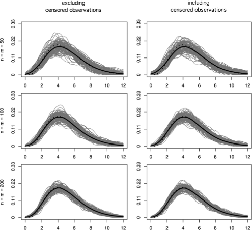
Figure 1: Overlayed sample paths.

5.2 Small-sample simulation results: Implementation and efficiency

To provide some illustration of the behavior of the methods proposed, we present below results from a preliminary small-sample simulation study. The objective was to graphically evaluate the general adequacy of the estimators as well as to elucidate the potential contribution of censored observations to overall estimation efficiency, both in small samples. For this purpose, we considered data emanating from the multiplicative censoring model, with underlying Gamma density function $g_{\alpha}(x)=\Gamma(\alpha)^{-1}x^{\alpha-1}\exp(-x)\mathbb{I}_{(0,\infty)}(x)$, various sample sizes and differing values of parameter $\alpha$. We found the kernel density estimators proposed to perform generally well. Figure 1 presents 100 sample paths, shown in grey, for various sample sizes and parameter value $\alpha=5$. Plots in the first column were obtained by discarding all censored observations and performing kernel density estimation using the uncensored observations alone; all observations were used in generating plots in the second column. The pointwise average of the sample plots is shown in solid black, while the true density is the dotted black curve depicted. The first, second and third rows were generated from datasets of 100, 200 and 400 total observations, respectively, with censored and uncensored observations equally represented. In all cases, bandwidth values were automatically selected using the $\Gamma(4,\beta)$ parametric reference rule (13). The Epanechnikov kernel $K(x)=\frac{3}{4}(1-x^{2})\mathbb{I}_{(-1,1)}(x)$ was used throughout. From these plots, we notice that use of the full sample leads to a decrease in variability throughout the support. Our empirical findings suggest that this cumulates to a substantial decrease in integrated squared error. Table 1 reports estimates and associated 95% confidence intervals for the mean relative difference in ISE, defined as $(\mbox{ISE}_{0}-\mbox{ISE}_{1})/\mbox{ISE}_{1}$, obtained from a simulation of 500 datasets, where $\mbox{ISE}_{0}$ and $\mbox{ISE}_{1}$ are the integrated squared errors associated with the use of the uncensored subsample and of the full sample, respectively. These values describe the mean percent increase in ISE from discarding the censored subsample, for various sample sizes and parameter values.

Table 1: Average percent increase in ISE and 95% CIs using $\Gamma(4,\beta)$ parametric reference rule

Sample size	$\bolds{\alpha=3}$	$\bolds{\alpha=4}$	$\bolds{\alpha=5}$	$\bolds{\alpha=6}$
$50+50$	${}_{15.2}17.1{}_{19.0}$	${}_{11.3}13.4{}_{15.6}$	${}_{16.4}18.4{}_{20.4}$	${}_{13.9}16.3{}_{18.7}$
$100+100$	${}_{16.8}18.5{}_{20.2}$	${}_{14.1}15.8{}_{17.5}$	${}_{13.6}15.3{}_{17.0}$	9${}_{9.9}11.6{}_{13.2}$
$200+200$	${}_{13.2}14.7{}_{16.1}$	${}_{11.6}13.1{}_{14.7}$	${}_{14.4}17.8{}_{21.2}$	${}_{18.4}22.6{}_{26.7}$

The relative performance of the estimators was found to be rather insensitive to the proximity of the underlying distribution to the parametric model specified in the reference rule used, with an average increase in ISE of around 10–25%, subsequent to discarding censored observations, regardless of sample size and parameter value. Since the performance of kernel density estimators hinges upon the performance of the underlying estimator of the distribution function as well as the adequacy of the bandwidth selection rule, gauging the contribution of censored observations to overall estimation efficiency is complicated by the layer of uncertainty associated to bandwidth selection. As such, we have also conducted a simulation study, whereby, for each simulated dataset, the bandwidth selected was that minimizing the observed ISE; we refer to this rule as the optimal bandwidth selection rule. Of course, such a rule can only be adopted in simulation settings, where the true density function is known, and the ISE can be computed directly. This approach provides, nonetheless, a clearer view of the gains resulting from the inclusion of censored observations in the estimation procedure. Table 2 reports estimates of the mean relative increase in ISE resulting from discarding all censored observations along with associated 95% confidence intervals. These results seem to suggest that for small and moderate sample sizes, when equal numbers of censored and uncensored observations are available, ignoring censored observations leads to an increase in ISE of roughly 10–35%, results consistent with those reported in Table 1.

Table 2: Average percent increase in ISE and 95% CIs using optimal bandwidth selection rule

Sample size	$\bolds{\alpha=3}$	$\bolds{\alpha=4}$	$\bolds{\alpha=5}$	$\bolds{\alpha=6}$
$50+50$	9${}_{9.6}14.3{}_{19.0}$	${}_{10.9}15.7{}_{20.5}$	9${}_{9.8}14.8{}_{19.9}$	${}_{17.3}32.5{}_{47.7}$
$100+100$	${}_{12.7}16.3{}_{20.0}$	${}_{12.9}17.3{}_{21.6}$	${}_{11.1}15.8{}_{20.5}$	${}_{12.4}26.9{}_{41.3}$
$200+200$	${}_{10.0}13.8{}_{17.6}$	${}_{12.1}17.2{}_{22.4}$	${}_{14.3}21.0{}_{27.7}$	${}_{16.9}34.6{}_{52.3}$

The above provides a glimpse of the contribution of the censored observations in small and moderate samples. It suggests that these observations provide nonnegligible information regarding the estimand of interest. We may, however, also resort to asymptotic arguments to motivate use of the full sample for the sake of efficiency. For any given distribution function $H$, denote the integrated squared error by

$$\mbox{ISE}(H,h;g)=\int\biggl{[}\frac{1}{h}\int K\biggl{(}\frac{x-y}{h}\biggr{)}\,dH(y)-g(y)\biggr{]}^{2}\,dy$$

and define the optimal bandwidth $\lambda(H;g)$ as the minimizer of the ISE with respect to the true density $g$, that is, $\lambda(H;g)=\mathop{\arg\min}_{h>0}\mbox{ISE}(H,h;g)$. Let $G_{m,n}$ be any consistent estimator of $G$ based on $(\mathcal{X}_{m},\mathcal{Y}_{n})$. The optimal kernel density estimator of $g$ based on $G_{m,n}$ is then $g^{\star}_{m,n}=\omega(G_{m,n})$, where $\omega$ is the operator defined pointwise as

$$\omega(H)(x)=\frac{1}{\lambda(H;g)}\int K\biggl{(}\frac{x-u}{\lambda(H;g)}\biggr{)}\,dH(u).$$

Since any solution $\hat{G}$ of the nonparametric score equation is asymptotically efficient for $G$ (see vardi1992lannals ), it is possible to show, along the lines of Theorem 25.47 of vandervaart2000 , that $\hat{g}_{m,n}^{\star}=\omega(\hat{G})$ is asymptotically efficient for $g=\omega(G)$. In particular, the kernel density estimator using the empirical distribution function based on uncensored observations alone cannot be expected to be asymptotically efficient, given that the latter is itself not efficient for $G$. It is thus clear that, barring additional complications linked to bandwidth selection, use of the full sample is preferable to that of the uncensored subsample alone.

6 Length-biased sampling with right-censoring

As discussed in theIntroduction, the likelihood of length-biased right-censored data is a particular case of that exhibited in (2). The literature on length-biased sampling can be traced as far back as wicksell1925biometrika , with important contributions by Fisher fisher1934ema , Neyman neyman1955science and Zelen zelen1969biometrika in medical applications, and by Cox cox1969ssp in industrial applications. The rigorous treatment of biased sampling was initiated in the 1980s by Vardi vardi1982annals , vardi1985annals , and furthered by Gill, Vardi and Wellner gill1988lannals , Vardi and Zhang vardi1992lannals , Bickel and Ritov bickel1991lannals , Gilbert gilbert2000annals and, more recently, by Asgharian, M’Lan and Wolfson asgharian2002jasa , Asgharian and Wolfson asgharian2005annals and Bergeron, Asgharian and Wolfson bergeron2008jasa . The importance of biased sampling in medical applications and prevalent cohort studies was re-emphasized by Cox and Oakes cox1984book .

The lifetime data typically collected on a prevalent cohort consist of triples $(A,R\wedge D,\Delta)$, where $A,R$ and $D$ are, respectively, the current-age, the residual lifetime and the residual censoring time, while $\Delta=\mathbb{I}_{\{R\leq D\}}$ is the censoring indicator. Suppose that $D$ and $(A,R)$ are independent. In one scenario considered in asgharian2005annals , all analyses are carried out conditionally upon the proportion of uncensored individuals, assumed fixed. As such, the observations are comprised of

$$(A_{i},R_{i})\stackrel{{\scriptstyle\mathrm{i.i.d.}}}{{\sim}}f_{A,R\mid\Delta=1},\qquad i=1,\ldots,m,$$

and

$$(A_{j},D_{j})\stackrel{{\scriptstyle\mathrm{i.i.d.}}}{{\sim}}f_{A,D\mid\Delta=0},\qquad j=1,\ldots,n,$$

where $f_{A,R}(a,r)=f_{U}(a+r)/\mu_{U}$ and $f_{U}$ is the probability density function associated to

$$F_{U}(t)=\int_{0}^{t}{s^{-1}\,dG(s)}{\Big{/}}\int_{0}^{\infty}{s^{-1}\,dG(s)}.$$ (14)

The conditional density functions above are explicitly given by

$$f_{A,R\mid\Delta=1}(a,r)=\frac{1-F_{D}(r)}{p(a+r)}\,dG(a+r)$$

and

$$f_{A,D\mid\Delta=0}(a,d)=\frac{f_{D}(d)}{(1-p)}\int_{a+d\leq z}z^{-1}\,dG(z)$$

for the uncensored and censored subjects, respectively. Here, $f_{D}$ and $F_{D}$ are, respectively, the density and distribution functions associated to the residual censoring random variable $D$, and $p=\mathrm{pr}(\Delta=1)$ is the proportion of uncensored individuals. The full likelihood of $m$ uncensored and $n$ censored length-biased observations is thus

$$\mathcal{L} = \prod_{i=1}^{m}{\biggl{[}\frac{1-F_{D}(r_{i})}{px_{i}}\,dG(x_{i})\biggr{]}}\prod_{j=1}^{n}\biggl{[}\frac{f_{D}(d_{j})}{1-p}\int_{y_{j}\leq z}z^{-1}\,dG(z)\biggr{]}$$

$$\propto \prod_{i=1}^{m}\,dG(x_{i})\prod_{j=1}^{n}\int_{y_{j}\leq z}z^{-1}\,dG(z).$$

Denoting $G_{\ast}(t)=P(A+R\leq t\mid\Delta=1)$ and $F_{\ast}(t)=P(A+D\leq t\mid\Delta=0)$ with associated density functions $g_{\ast}(t)$ and $f_{\ast}(t)$, we may verify that

$$g_{\ast}(t)=\frac{g(t)}{pt}\int_{0}^{t}{[1-F_{D}(r)]\,dr}\quad\mbox{and}\quad f_{\ast}(t)=\frac{f(t)F_{D}(t)}{1-p},$$

where $f(t)$ is given by (1). Defining the operators

$$\mathcal{H}(u)(t) = \int_{0<x\leq t}\frac{g_{\ast}(x)}{g(x)}\,du(x),$$

$$\mathcal{K}_{m,n}(u)(t) = \int_{0<y\leq t}y\biggl{(}\int_{y\leq z}\frac{u(z)}{z^{2}}\,dz\biggr{)}\,d\biggl{[}\biggl{(}\frac{\hat{f}(t)}{\hat{f}(y)}-1\biggr{)}\frac{f_{\ast}(y)}{f(y)}\biggr{]}$$

and $\Psi_{m,n}=\hat{p}\mathcal{H}+(1-\hat{p})\mathcal{K}_{m,n}$, Asgharian and Wolfson asgharian2005annals have derived, under this scenario, the equation $\Psi_{m,n}(U_{m,n})=W_{m,n}$, where $W_{m,n}$ is obtained from (4) by replacing $W_{X,m}$ and $W_{Y,n}$ by the empirical processes $\sqrt{m}(G_{m}-G_{*})$ and $\sqrt{n}(F_{n}-F_{*})$, respectively. Defining the limiting operators

$$\mathcal{K}(u)(t)=\int_{0<y\leq t}y\biggl{(}\int_{y\leq z}\frac{u(z)}{z^{2}}\,dz\biggr{)}\,d\biggl{[}\biggl{(}\frac{f(t)}{f(y)}-1\biggr{)}\frac{f_{\ast}(y)}{f(y)}\biggr{]}$$

and $\Psi=p\mathcal{H}+(1-p)\mathcal{K}$, one can show that $\Psi_{m,n}$ converges almost surely to $\Psi$ in operator norm topology, and that $\Psi$ is bounded, linear and has bounded inverse $\Psi^{-1}$ if $p>0.59$; see asgharian2005annals .

As discussed in the Introduction, when the observation mechanism generates length-biased samples, it is often of prime interest to make inference about $F_{U}$ and its density function $f_{U}$. Substitution of $G$ by $\hat{G}$ in (14) yields $\hat{F}_{U}$, an asymptotically efficient estimator of $F_{U}$. The asymptotic properties of $Z_{m,n}=\sqrt{k}(\hat{F}_{U}-F_{U})$ may be studied via its relation to $U_{m,n}$. Indeed, defining $L_{t}(x)=x^{-1}[\mathbb{I}_{[0,t]}(x)-F_{U}(t)]$, we may write

$$\hat{F}_{U}(s)-F_{U}(s)=\frac{\int_{0}^{\infty}L_{s}(x)\,d[\hat{G}(x)-G(x)]}{\int_{0}^{\infty}x^{-1}\,d\hat{G}(x)},$$

from which we have that $Z_{m,n}=\int_{0}^{\infty}{L_{s}(x)\,dU_{m,n}(x)}/\int_{0}^{\infty}{x^{-1}\,d\hat{G}(x)}$. Defining the operator $\mathscr{L}(g)(t)=\mu_{U}^{-1}\int_{0}^{\infty}L_{t}(x)\,dg(x)$, we note that if there exists some $\gamma_{0}>0$ such that $G(\gamma_{0})=0$ (in which case $G$ is said to satisfy assumption $\gamma$), the operator $\mathscr{L}$ is bounded. Consequently, Theorems 1–5 hold when making inference about $F_{U}$ and its density function $f_{U}$.

Under the additional assumption that the residual censoring distribution does not have a point-mass at zero, it is possible to provide an explicit distributional result for the empirical density process arising from kernel density estimation. Specifically, we have that the empirical density process $\sqrt{kh_{m,n}}(\hat{f}_{U}-f_{U})$ is asymptotically Gaussian with mean zero and covariance function $\sigma_{f_{U}}$ estimated consistently by

$$\hat{\sigma}_{f_{U}}(s,t)=h_{m,n}^{-1}\int\!\!\int{\hat{\psi}_{Z}(s-uh_{m,n},t-vh_{m,n})\,dK(u)\,dK(v)},$$

where $\hat{\psi}_{Z}$ is a consistent estimator of the asymptotic covariance function $\psi_{Z}$ associated to the sequence of processes $Z_{m,n}$. For example, we may take

$$\hat{\psi}_{Z}(s,t)=\hat{\mu}_{U}^{-2}\int\!\!\int{\hat{\psi}_{U}(x,y)\,d\hat{L}_{s}(x)\,d\hat{L}_{t}(y)},$$

where $\hat{\mu}_{U}=\int_{0}^{\infty}{z^{-1}\,d\hat{G}(z)}$, $\hat{L}_{u}(z)=z^{-1}[\mathbb{I}_{[0,u]}(z)-\hat{F}_{U}(z)]$ and $\hat{\psi}_{U}$ is a consistent estimator of the covariance function $\psi_{U}$ of process $U$. Since for $s\leq t$ we may write $\psi_{U}(s,t)$ as

$$p\biggl{\{}\int_{0}^{s}{[\beta(x)]^{2}\,dG_{*}(x)}-\biggl{[}\int_{0}^{s}{\beta(x)\,dG_{*}(x)}\int_{0}^{t}{\beta(x)\,dG_{*}(x)}\biggr{]}\biggr{\}}$$

$$\quad{}+(1-p)\int_{0}^{t}\int_{0}^{s}f(x)f(y)\biggl{\{}e(x\wedge y)$$

$$\hskip 136.5pt{}+h(x\wedge y)\biggl{[}\frac{1}{f(x\vee y)}-\frac{1}{f(x\wedge y)}\biggr{]}$$

$$\hskip 241.0pt{}-h(x)h(y)\biggr{\}}\,d\zeta(x)\,d\zeta(y),$$

where we have defined $\zeta(x)=g(x)[pg_{*}(x)]^{-1}$, $h(x)=\int_{0}^{x}{F_{*}(y)\,d[1/f(y)]}$ and $e(x)=2\int_{0}^{x}{h(y)\,d[1/f(y)]}$, consistent estimation of $\psi_{U}$ is possible by substitution of appropriate empirical counterparts into the above.

Assumption $\gamma$ imposed on $G$ may seem restrictive, but nonetheless holds in many industrial and medical applications. The case of survival with dementia, studied in asgharian2002jasa and wolfson2001nejm , is an example of such. It is possible to relax this requirement by imposing that $G$ and $F_{D}$ vanish at zero at a super-polynomial rate, that is, by assuming that $G(t)$ and $F_{D}(t)$ are $o(t^{r})$ as $t\rightarrow 0$ for each $r>0$. While preserving all results pertaining to $G$, this relaxation does not directly preserve those pertaining to $F_{U}$. The unboundedness of $\mathscr{L}$ is problematic, although an application of Tikhonov’s regularization method may help in circumventing this problem. This has been explored by Carroll, Rooij and Ruymgaart carroll1991aam , although not from the perspective of strong approximations.

7 Closing remarks

(1) For distributions with a lighter left tail ($\alpha_{0}>2$) and heavier right tail (small $\beta$), the rate obtained for the strong approximation of $U_{m,n}$ is close to $k^{-1/4}$ modulo logarithmic terms. It is unclear whether it is possible to achieve better rates; if so, different techniques would necessarily be needed to control the rate of $\mathcal{I}_{5}$ in Lemma 4, as the best achievable rate for $\mathcal{I}_{5}$ using approximations by Bernstein polynomials is $k^{-1/4}$. As for assumption (B2) on the bandwidth required to establish Theorem 3, the $k^{-1/4}$ rate in the strong approximation roughly translates into the bandwidth condition $(\log k)^{2}/(k^{3/4}h_{m,n})\to 0$ when we further replace the iterated logarithmic term by a logarithmic term. This is in contrast to $\log k/(kh_{m,n})\rightarrow 0$ obtained in silverman1978annals , in the case of uncensored observations alone. Likewise, the rate given in Remark 2, after Theorem 4, is roughly $h_{m,n}\sim(\log k)^{2/3}/k^{1/4}$.

(2) The theory presented in this paper requires that $\hat{p}\rightarrow p\in(0,1]$. The case $p=0$ may itself be of interest. On one hand, if $\hat{p}=0$ for each $k$, then all observations are multiplicatively censored; this has been studied by Groeneboom groeneboom1985berkconf , among others. On the other hand, if $\hat{p}>0$ for each $k$, the methods developed in this paper may be adapted as long as $\hat{p}$ does not vanish too rapidly. Specifically, we may redefine $\mathcal{F}_{m,n}=\hat{p}\mathcal{I}+(1-\hat{p})\mathcal{G}$ and

$$W^{0}_{m,n}(s)=\sqrt{\hat{p}}B_{X,m}(G(s))+\sqrt{1-\hat{p}}f(s)\int_{0<y\leq s}B_{Y,n}(F(y))\,d\biggl{[}\frac{1}{f(y)}\biggr{]}.$$

Suppose that $\hat{p}^{-2}$ is $\mathcal{O}(\upsilon_{k})$ for some sequence of positive real numbers $\upsilon_{k}$ tending to infinity. Then the strong approximation holds, with $U^{0}_{m,n}$ redefined as the Gaussian process $\mathcal{F}_{m,n}^{-1}(W^{0}_{m,n})$ and the rates being multiplied by $\mathcal{O}(\upsilon_{k}^{2})$. Further, the rate of the global modulus of continuity of $U^{0}_{m,n}$ is multiplied by $\mathcal{O}(\upsilon_{k})$. This allows one to study the case $p=0$. This extension provides insight into the leap between the square-root asymptotics in the canonical multiplicative censoring setting and the cube-root asymptotics for the Grenander estimator when only censored observations are available.

Appendix: Proofs of main results

Proof of Claim 1 If the condition $\sum_{m,n}G(\gamma_{m,n})<\infty$ is satisfied, it is an immediate consequence of Theorem 1 of Section 10.1 of shorack1986 that $\mathrm{pr}(\min(X_{1},\ldots,X_{m})\leq\gamma_{m,n}\mbox{ i.o.})=0$. Hence, almost surely, we may find $m_{0}$ and $n_{0}\in\mathbb{N}$ such that, for each $m\geq m_{0}$ and $n\geq n_{0}$, all uncensored observations $x_{1},\ldots,x_{m}$ are no smaller than $\gamma_{m,n}$. We restrict our attention here to such sufficiently large $m$ and $n$. Define $\delta_{i}=\mathbb{I}_{\{x_{1},\ldots,x_{m}\}}(t_{i})$ for $i=1,\ldots,k$, and write $r_{0}=\min\{i\dvtx t_{i}\geq\gamma_{m,n}\}$. By construction, we must have that $\delta_{1}=\cdots=\delta_{r_{0}-1}=0$. Define the set

$$\mathscr{D}=\Biggl{\{}(a_{r_{0}},a_{r_{0}+1},\ldots,a_{k})\dvtx 0\leq a_{r_{0}},a_{r_{0}+1},\ldots,a_{k}\leq 1,\sum_{i=r_{0}}^{k}a_{i}=1,a_{k}\geq\frac{1}{k}\Biggr{\}},$$

a bounded, closed and convex subset of $\mathbb{R}^{k-r_{0}+1}$. For $i=r_{0},\ldots,k$, define

$$\phi_{i}(a_{r_{0}},\ldots,a_{k}) = \delta_{i}\biggl{(}\frac{\hat{p}}{m}\biggr{)}+\frac{a_{i}}{t_{i}}\biggl{(}\frac{1-\hat{p}}{n}\biggr{)}\sum_{j=1}^{i}{\frac{1-\delta_{j}}{\sum_{q=\max(j,r_{0})}^{k}a_{q}/t_{q}}}$$

$$= \frac{1}{k}\Biggl{(}\delta_{i}+\frac{a_{i}}{t_{i}}\sum_{j=1}^{i}{\frac{1-\delta_{j}}{\sum_{q=\max(j,r_{0})}^{k}a_{q}/t_{q}}}\Biggr{)}$$

and $\phi=(\phi_{r_{0}},\ldots,\phi_{k})$. We note that $\phi$ is continuous on $\mathscr{D}$. We want to show that $\phi(\mathscr{D})\subseteq\mathscr{D}$. The fact that the image of $\mathscr{D}$ under $\phi_{i}$ is contained in $[0,1]$ for $i=r_{0},\ldots,k$ is clear. That it is contained in $[1/k,1]$ for $i=k$ is obvious if $\delta_{k}=1$. We assume instead that $\delta_{k}=0$. Then, defining $\lambda_{j}=\sum_{q=\max(j,r_{0})}^{k-1}a_{q}/t_{q}\geq 0$ for $j=1,\ldots,k-1$ and $\lambda_{k}=a_{k}/t_{k}\geq 0$, we observe that

$$\frac{a_{k}}{t_{k}}\sum_{j=1}^{k}{\frac{1-\delta_{j}}{\sum_{q=\max(j,r_{0})}^{k}a_{q}/t_{q}}}=\lambda_{k}\Biggl{(}\sum_{j=1}^{k-1}{\frac{1-\delta_{j}}{\lambda_{j}+\lambda_{k}}}+\frac{1}{\lambda_{k}}\Biggr{)}\geq 1,$$

from which it follows that the image of $\mathscr{D}$ under $\phi_{k}$ is contained in $[1/k,1]$ if $\delta_{k}=0$ as well. Finally, we require the equality $\sum_{i=r_{0}}^{k}{\phi_{i}(a_{r_{0}},\ldots,a_{k})}=1$ to hold for any $(a_{r_{0}},\ldots,a_{k})\in\mathscr{D}$. This can be verified using that

$$\sum_{i=r_{0}}^{k}\sum_{j=1}^{i}b_{ij}=\sum_{j=1}^{r_{0}-1}\sum_{i=r_{0}}^{k}{b_{ij}}+\sum_{j=r_{0}}^{k}\sum_{i=j}^{k}{b_{ij}}$$

for any array $b_{ij}$, where under the first sum on the right-hand side, it holds that $\max(j,r_{0})=r_{0}$, while under the second sum, $\max(j,r_{0})=j$. We may thus use the Brouwer fixed point theorem (see, e.g., Proposition 2.6 on page 52 and Problem 6.7e on page 254 of zeidler1985 ) to obtain that there exists some $a^{*}=(a_{r_{0}}^{*},\ldots,a_{k}^{*})\in\mathscr{D}$ such that $\phi(a^{*})=a^{*}$. The distribution function

$$\hat{G}^{*}(t)=\sum_{i=r_{0}}^{k}a^{*}_{i}\mathbb{I}_{[0,t]}(t_{i})$$

is a solution to equation (3) with zero mass below $\gamma_{m,n}$. Proof of Theorem 1 Using Lemma 1 and the boundedness of $\mathcal{F}_{m,n}^{-1}$, we have for each $t\in[0,\tau-\varepsilon]$ that

$$U_{m,n}(t)=\mathcal{F}_{m,n,\varepsilon}^{-1}(W_{m,n})(t)+\mathcal{O}\bigl{(}\varepsilon\sqrt{\log\log k}\bigr{)}\qquad\mbox{a.s.}$$

Similarly, using the definition of $U_{m,n}^{0}$, $W_{m,n}^{0}$, Lemma 6 and the boundedness of $\mathcal{F}^{-1}$, we have for each $t\in[0,\tau-\varepsilon]$ that

$$U_{m,n}^{0}(t)=\mathcal{F}_{\varepsilon}^{-1}(W_{m,n}^{0})(t)+\mathcal{O}\bigl{(}\varepsilon\sqrt{\log k}\bigr{)}\qquad\mbox{a.s.}$$

The result follows from Lemmas 3, 5 and 6 and the inequality

$$\|U_{m,n}-U_{m,n}^{0}\|_{[0,\tau-\varepsilon]} = \|{\mathcal{F}}_{m,n}^{-1}(W_{m,n})-{\mathcal{F}}^{-1}(W_{m,n}^{0})\|_{[0,\tau-\varepsilon]}$$

$$\leq \|{\mathcal{F}}_{m,n,\varepsilon}^{-1}\|\|W_{m,n}-W_{m,n}^{0}\|_{[0,\tau-\varepsilon]}$$

$${}+\|\mathcal{F}_{m,n,\varepsilon}^{-1}-\mathcal{F}^{-1}_{\varepsilon}\|\|W_{m,n}^{0}\|_{[0,\tau-\varepsilon]}$$

$${}+\mathcal{O}\bigl{(}\varepsilon\sqrt{\log k}\bigr{)}\qquad\mbox{a.s.}$$

We therefore find that

$$\|U_{m,n}-U_{m,n}^{0}\|_{[0,\tau-\varepsilon]} \leq \mathcal{O}\biggl{(}\frac{k^{-r(\alpha)}\sqrt{\log k}(\log\log k)^{{1}/{4}}}{f(\tau-\varepsilon)}\biggr{)}$$

$${}+\mathcal{O}\biggl{(}\frac{k^{-({\alpha-1})/({2\alpha})}\log k\sqrt{\log\log k}}{f(\tau-\varepsilon)}\biggr{)}\mathcal{O}\bigl{(}\sqrt{\log k}\bigr{)}$$

$${}+\mathcal{O}\bigl{(}\varepsilon\sqrt{\log k}\bigr{)}\qquad\mbox{a.s.}$$

The use of Lemma 3 was justified by the fact that $W^{0}_{m,n}$ is almost surely continuous. Since (A4) implies that $f(\tau-u)\sim u^{\beta}$ for $u$ small, the above bound has least order, modulo logarithmic terms, for $\varepsilon=\varepsilon_{m,n}$. Proof of Theorem 2 Let $t\in[0,\tau-\eta]$ and $s\in[0,h_{m,n}]$. By definition (10), linearity of $\mathcal{F}^{-1}$ and the triangle inequality, we have that

$$|U^{0}_{m,n}(t+s)-U^{0}_{m,n}(t)|\leq I_{m}(s,t)+J_{n}(s,t),$$ (15)

where we define

$$I_{m}(s,t) = |\mathcal{F}^{-1}(B_{X,m}\circ G)(t+s)-{\mathcal{F}^{-1}(B_{X,m}\circ G)(t)}|,$$

$$J_{n}(s,t) = |\mathcal{F}^{-1}(\mathcal{H}_{n})(t+s)-\mathcal{F}^{-1}(\mathcal{H}_{n})(t)|$$

and

$$\mathcal{H}_{n}(t)=f(t)\int_{0<y\leq t}B_{Y,n}(F(y))\,d\biggl{[}\frac{1}{f(y)}\biggr{]}.$$

We first study $I_{m}(s,t)$. Writing $\varsigma(u)(\cdot)=\int_{0}^{\infty}{K(\cdot,x)u(x)\,dx}$ and noting that $\int_{0}^{\infty}{\mathcal{A}_{0}(\cdot,x)u(x)\,dx}=\mathcal{G}(u)(\cdot)$ for each $u$, equations (8) and (9) imply that $\varsigma(u)\equiv-(1-p)\mathcal{G}(u+p\varsigma(u))/p^{2}$. It follows from (A5) that $M_{1}=\|f^{\prime}\|_{[0,\tau]}<\infty$. We find that

$$|\mathcal{G}(w)(t+s)-\mathcal{G}(w)(s)|$$

$$\qquad\leq|f(t+s)-f(t)|\biggl{|}\int_{0<y\leq t}y\biggl{(}\int_{y\leq z}\frac{w(z)}{z^{2}}\,dz\biggr{)}\,d\biggl{[}\frac{1}{f(y)}\biggr{]}\biggr{|}$$

$$\qquad\quad{}+|f(t)|\biggl{|}\int_{t<y\leq t+s}y\biggl{(}\int_{y\leq z}\frac{w(z)}{z^{2}}\,dz\biggr{)}\,d\biggl{[}\frac{1}{f(y)}\biggr{]}\biggr{|}$$

$$\qquad\leq|f(t+s)-f(t)|\biggl{[}\frac{1}{f(t)}-\frac{1}{f(0)}\biggr{]}\|w\|_{[0,\tau]}$$

$$\qquad\quad{}+|f(t+s)|\biggl{[}\frac{1}{f(t+s)}-\frac{1}{f(t)}\biggr{]}\|w\|_{[0,\tau]}$$

$$\qquad=|f(t+s)-f(t)|\biggl{[}\frac{f(0)-f(t)}{f(0)f(t)}+\frac{1}{f(t)}\biggr{]}\|w\|_{[0,\tau]}$$

$$\qquad\leq\frac{2}{f(\tau-\eta)}\|w\|_{[0,\tau]}|f(t+s)-f(t)|$$

$$\qquad\leq\frac{2M_{1}s}{f(\tau-\eta)}\|w\|_{[0,\tau]}$$

from which it follows, using (7), that

$$|\varsigma(u)(t+s)-\varsigma(u)(t)| \leq \frac{2(1-p)M_{1}s}{p^{2}f(\tau-\eta)}\|u+p\varsigma(u)\|_{[0,\tau]}$$

$$\leq \frac{2(1-p)M_{1}s}{p^{2}f(\tau-\eta)}(2+p\|\mathcal{F}^{-1}\|)\|u\|_{[0,\tau]}.$$

Using (7) once more, we then have that

$$\sup_{0\leq t\leq\tau-\eta}\sup_{0\leq s\leq h_{m,n}}I_{m}(s,t)$$

$$\qquad\leq p^{-1}\sup_{0\leq t\leq\tau-\eta}\sup_{0\leq s\leq h_{m,n}}\bigl{|}B_{X,m}\bigl{(}G(t+s)\bigr{)}-B_{X,m}(G(t))\bigr{|}$$

$$\qquad\quad{}+\sup_{0\leq t\leq\tau-\eta}\sup_{0\leq s\leq h_{m,n}}|\varsigma(B_{X,m}\circ G)(t+s)-\varsigma(B_{X,m}\circ G)(t)|.$$

Using (A5), we may show, as in mason1983probtheory and shorack1986 , that

$${\sup_{0\leq x\leq a_{\tau}}\sup_{0\leq y\leq M_{0}h_{m,n}}}|\mathcal{W}_{X,m}(x+y)-\mathcal{W}_{X,m}(x)|=\mathcal{O}\bigl{(}\sqrt{h_{m,n}\log(1/h_{m,n})}\bigr{)}$$

almost surely, where $a_{\tau}=G(\tau-\eta)$, $M_{0}=\|g\|_{[0,\tau]}$, and $\mathcal{W}_{X,m}$ is the Wiener process associated with $B_{X,m}$; see Lemma 1.4.1 of csorgo1981 . Hence, by an application of the MVT, $B_{X,m}\circ G$ has modulus of continuity

$$\mathcal{O}\bigl{(}\sqrt{h_{m,n}\log(1/h_{m,n})}\bigr{)}$$

as well. In view of (Appendix: Proofs of main results) and the fact that $\|B_{X,m}\circ G\|_{[0,\tau]}$ is $\mathcal{O}(\sqrt{\log m})$ almost surely, we have that

$$\sup_{0\leq t\leq\tau-\eta}\sup_{0\leq s\leq h_{m,n}}|\varsigma(B_{X,m}\circ G)(t+s)-\varsigma(B_{X,m}\circ G)(t)|=\mathcal{O}\bigl{(}\sqrt{\log{m}}h_{m,n}\bigr{)}$$

almost surely. It follows from the discussion above then that

$$\sup_{0\leq t\leq\tau-\eta}\sup_{0\leq s\leq h_{m,n}}I_{m}(s,t)=\mathcal{O}\bigl{(}\sqrt{h_{m,n}\log(1/h_{m,n})}\bigr{)}\qquad\mbox{a.s.}$$ (17)

We now turn to $J_{n}(s,t)$. Defining

$$J^{\prime}_{n}(s,t)=|f(t+s)-f(t)|\int_{0<y\leq t}{|B_{Y,n}(F(y))|\,d\biggl{[}\frac{1}{f(y)}\biggr{]}}$$

and

$$J^{\prime\prime}_{n}(s,t)=|f(t+s)|\int_{t<y\leq t+s}{|B_{Y,n}(F(y))|\,d\biggl{[}\frac{1}{f(y)}\biggr{]}},$$

we notice that $|\mathcal{H}_{n}(t+s)-\mathcal{H}_{n}(t)|\leq J^{\prime}_{n}(s,t)+J^{\prime\prime}_{n}(s,t)$. Using the MVT, we have that

$$J^{\prime}_{n}(s,t)\leq{\frac{M_{1}s}{f(\tau-\eta)}\sup_{0\leq y\leq 1}}{|B_{Y,n}(y)|}$$

and

$$J^{\prime\prime}_{n}(s,t)\leq{\frac{f(t)-f(t+s)}{f(t)}\sup_{0\leq y\leq 1}}{|B_{Y,n}(y)|}\leq{\frac{M_{1}s}{f(t)}\sup_{0\leq y\leq 1}}{|B_{Y,n}(y)|},$$

so that $\sup_{0\leq t\leq\tau-\eta}\sup_{0\leq s\leq h_{m,n}}J^{\prime}_{n}(s,t)$, $\sup_{0\leq t\leq\tau-\eta}\sup_{0\leq s\leq h_{m,n}}J^{\prime\prime}_{n}(s,t)$ and consequently ${\sup_{0\leq t\leq\tau-\eta}\sup_{0\leq s\leq h_{m,n}}}|\mathcal{H}_{n}(t+s)-\mathcal{H}_{n}(t)|$ are $\mathcal{O}(\sqrt{\log{n}}h_{m,n})$ almost surely. Further, using (Appendix: Proofs of main results), we have that

$${\sup_{0\leq t\leq\tau-\eta}\sup_{0\leq s\leq h_{m,n}}}|\varsigma(\mathcal{H}_{n})(t+s)-\varsigma(\mathcal{H}_{n})(t)|$$

$$\qquad\leq\frac{2(1-p)M_{1}}{p^{2}f(\tau-\eta)}(2+p\cdot\|\mathcal{F}^{-1}\|)\|\mathcal{H}_{n}\|_{[0,\tau]}h_{m,n}=\mathcal{O}\bigl{(}\sqrt{\log n}h_{m,n}\bigr{)}\qquad\mbox{a.s.}$$

so that $\sup_{0\leq t\leq\tau-\eta}\sup_{0\leq s\leq h_{m,n}}J_{n}(s,t)=\mathcal{O}(\sqrt{\log n}h_{m,n})$ almost surely using (7). The theorem follows in view of this last result, (15) and (17). Proof of Theorem 3 By the continuity (and hence uniform continuity) of $g$ on $[0,\tau]$, the dominated convergence theorem may be used to show that

$${\lim_{k\rightarrow\infty}}\sup_{0\leq s\leq\tau-\eta}|g_{m,n}(s)-g(s)|=0.$$ (18)

The theorem follows immediately from Lemma 7 and the triangle inequality. Proof of Theorem 4 By Theorem 1 and integration by parts, for any $t\in[0,\tau-\eta]$, we may write that

$$\hat{g}_{m,n}(t)-g(t) = [\hat{g}_{m,n}(t)-g_{m,n}(t)]+[g_{m,n}(t)-g(t)]$$

$$= \frac{1}{\sqrt{k}}\int_{0}^{\infty}{U_{m,n}^{0}(s)\,d\psi_{m,n}(t,s)}$$

$${}+\mathcal{O}\biggl{(}\frac{V_{m,n}\varepsilon_{m,n}(\log k)^{{3}/{2}}\sqrt{\log\log k}}{\sqrt{k}}+\delta_{m,n}\biggr{)}\qquad\mbox{a.s.},$$

where $\delta_{m,n}=\sup_{0\leq t\leq\tau-\eta}|g_{m,n}(t)-g(t)|$. The result follows from Rev72 , which shows that $\delta_{m,n}=\mathcal{O}(h^{2}_{m,n})$ and $V_{m,n}=\mathcal{O}(1/h_{m,n})$. Proof of Theorem 5 Since $g$ is twice continuously differentiable on $[0,\tau-\eta]$, we may write that $g_{m,n}(s)-g(s)=h_{m,n}^{2}\sigma^{2}g^{\prime\prime}(s)/2+o(h_{m,n}^{2})$ uniformly in $s\in[0,\tau-\eta]$. Combining this expansion with (S.1) in the proof of Lemma 7 (see supplementary material asgharian2012supp ) yields

$$\hat{g}_{m,n}(s)-g(s) = \biggl{(}\frac{h_{m,n}^{2}\sigma^{2}}{2}\biggr{)}g^{\prime\prime}(s)+\frac{\Upsilon_{m,n}(s,h_{m,n})}{\sqrt{k}h_{m,n}}$$

$${}+\mathcal{O}\biggl{(}\frac{\varepsilon_{m,n}(\log k)^{{3}/{2}}\sqrt{\log\log k}}{\sqrt{k}h_{m,n}}\biggr{)}+o(h_{m,n}^{2})\qquad\mbox{a.s.}$$

uniformly in $s\in[0,\tau-\eta]$, where $\Upsilon_{m,n}(s,h)=\int_{-1}^{1}{U_{m,n}^{0}(s-uh)\,dK(u)}$. In view of (7) and the proof of Theorem 2, we find that

$$\Upsilon_{m,n}(s,h_{m,n})=p^{-{1}/{2}}\int_{-1}^{1}B_{X,m}\bigl{(}G(s-uh_{m,n})\bigr{)}\,dK(u)+\mathcal{O}\bigl{(}\sqrt{\log k}h_{m,n}\bigr{)}\quad\mbox{a.s.}$$

Further, using (B3) we may show, for $\alpha\geq 2$, that

$$\frac{\varepsilon_{m,n}(\log k)^{{3}/{2}}\sqrt{\log\log k}}{\sqrt{k}h_{m,n}}=o(h_{m,n}^{2})$$

and therefore that

$$\hat{g}_{m,n}(s)-g(s)=\biggl{(}\frac{h_{m,n}^{2}\sigma^{2}}{2}\biggr{)}g^{\prime\prime}(s)+\frac{\int_{-1}^{1}B_{X,m}(G(s-uh))\,dK(u)}{\sqrt{pk}h_{m,n}}+o(h_{m,n}^{2})$$

almost surely. It then follows that $\mathcal{E}_{m,n}(0,\tau-\eta)$ may be written as

$$\frac{h_{m,n}^{4}\sigma^{4}}{4}\int_{0}^{\tau-\eta}{\{g^{\prime\prime}(s)\}^{2}\,ds}+\frac{{}_{\eta}P_{m,n}(h_{m,n})}{pkh_{m,n}^{2}}+\frac{\sigma^{2}h_{m,n}{}_{\eta}Q_{m,n}(h_{m,n})}{\sqrt{pk}}$$

$$\qquad{}+o(h_{m,n}^{2})\biggl{\{}o(h_{m,n}^{2})+h_{m,n}^{2}\sigma^{2}\int_{0}^{\tau-\eta}g^{\prime\prime}(s)\,ds+\frac{2_{\eta}R_{m,n}(h_{m,n})}{\sqrt{pk}h_{m,n}}\biggr{\}}\qquad\mbox{a.s.},$$

where we have defined

$${}_{\eta}P_{m,n}(h) = \int_{0}^{\tau-\eta}{\biggl{[}\int_{-1}^{1}B_{X,m}\bigl{(}G(s-uh)\bigr{)}\,dK(u)\biggr{]}^{2}\,ds},$$

$${}_{\eta}Q_{m,n}(h) = \int_{0}^{\tau-\eta}{g^{\prime\prime}(s)\biggl{[}\int_{-1}^{1}B_{X,m}\bigl{(}G(s-uh)\bigr{)}\,dK(u)\biggr{]}\,ds}$$

and

$${}_{\eta}R_{m,n}(h)=\int_{0}^{\tau-\eta}\biggl{[}\int_{-1}^{1}B_{X,m}\bigl{(}G(s-uh)\bigr{)}\,dK(u)\biggr{]}\,ds.$$

It follows from hall1982stochproc that ${}_{\eta}P_{m,n}(h)=h_{m,n}\nu^{2}+o_{p}(h_{m,n})$, while ${}_{\eta}Q_{m,n}(h)$ and ${}_{\eta}R_{m,n}(h)$ are both $o_{p}(\sqrt{h_{m,n}})$. We therefore obtain that $\mathcal{E}_{m,n}(0,\tau-\eta)$ may be expressed as

$$\frac{h_{m,n}^{4}\sigma^{4}}{4}\int_{0}^{\tau-\eta}{[g^{\prime\prime}(s)]^{2}\,ds}+\frac{\nu^{2}}{pkh_{m,n}}+o_{p}\Biggl{(}\frac{1}{kh_{m,n}}+h_{m,n}\sqrt{\frac{h_{m,n}}{k}}+h_{m,n}^{4}\Biggr{)}.$$

The result follows upon noticing that a term of order $o_{p}(h_{m,n}^{3/2}/\sqrt{k})$ is dominated by any term of order $o_{p}(h_{m,n}^{4})$.

References

- (1) {bmisc}[auto:STB—2012/01/18—07:48:53] \bauthor\bsnmAsgharian, \bfnmM.\binitsM., \bauthor\bsnmCarone, \bfnmM.\binitsM. and \bauthor\bsnmFakoor, \bfnmV.\binitsV. (\byear2012). \bhowpublishedSupplement to “Large-sample study of the kernel density estimators under multiplicative censoring.” DOI:10.1214/11-AOS954SUPP. \bptokimsref \endbibitem
- (2) {barticle}[mr] \bauthor\bsnmAsgharian, \bfnmMasoud\binitsM., \bauthor\bsnmM’Lan, \bfnmCyr Emile\binitsC. E. and \bauthor\bsnmWolfson, \bfnmDavid B.\binitsD. B. (\byear2002). \btitleLength-biased sampling with right censoring: An unconditional approach. \bjournalJ. Amer. Statist. Assoc. \bvolume97 \bpages201–209. \biddoi=10.1198/016214502753479347, issn=0162-1459, mr=1947280 \bptokimsref \endbibitem
- (3) {barticle}[mr] \bauthor\bsnmAsgharian, \bfnmMasoud\binitsM. and \bauthor\bsnmWolfson, \bfnmDavid B.\binitsD. B. (\byear2005). \btitleAsymptotic behavior of the unconditional NPMLE of the length-biased survivor function from right censored prevalent cohort data. \bjournalAnn. Statist. \bvolume33 \bpages2109–2131. \biddoi=10.1214/009053605000000372, issn=0090-5364, mr=2211081 \bptokimsref \endbibitem
- (4) {barticle}[mr] \bauthor\bsnmAsgharian, \bfnmMasoud\binitsM., \bauthor\bsnmWolfson, \bfnmDavid B.\binitsD. B. and \bauthor\bsnmZhang, \bfnmXun\binitsX. (\byear2006). \btitleChecking stationarity of the incidence rate using prevalent cohort survival data. \bjournalStat. Med. \bvolume25 \bpages1751–1767. \biddoi=10.1002/sim.2326, issn=0277-6715, mr=2227351 \bptokimsref \endbibitem
- (5) {barticle}[mr] \bauthor\bsnmBergeron, \bfnmPierre-Jérôme\binitsP.-J., \bauthor\bsnmAsgharian, \bfnmMasoud\binitsM. and \bauthor\bsnmWolfson, \bfnmDavid B.\binitsD. B. (\byear2008). \btitleCovariate bias induced by length-biased sampling of failure times. \bjournalJ. Amer. Statist. Assoc. \bvolume103 \bpages737–742. \biddoi=10.1198/016214508000000382, issn=0162-1459, mr=2524006 \bptokimsref \endbibitem
- (6) {bbook}[auto:STB—2012/01/18—07:48:53] \bauthor\bsnmBickel, \bfnmP. J.\binitsP. J., \bauthor\bsnmKlaassen, \bfnmA. J.\binitsA. J., \bauthor\bsnmRitov, \bfnmY.\binitsY. and \bauthor\bsnmWellner, \bfnmJ. A.\binitsJ. A. (\byear1993). \btitleEfficient and Adaptive Inference in Semiparametric Models. \bpublisherJohns Hopkins Univ. Press, \baddressBaltimore. \bptokimsref \endbibitem
- (7) {barticle}[mr] \bauthor\bsnmBickel, \bfnmPeter J.\binitsP. J. and \bauthor\bsnmRitov, \bfnmJ.\binitsJ. (\byear1991). \btitleLarge sample theory of estimation in biased sampling regression models. I. \bjournalAnn. Statist. \bvolume19 \bpages797–816. \biddoi=10.1214/aos/1176348121, issn=0090-5364, mr=1105845 \bptokimsref \endbibitem
- (8) {barticle}[mr] \bauthor\bsnmBikel, \bfnmP. Dzh.\binitsP. D. and \bauthor\bsnmRitov, \bfnmI.\binitsI. (\byear1994). \btitleEfficient estimation using both direct and indirect observations. \bjournalTheory Probab. Appl. \bvolume38 \bpages194–213. \bptokimsref \endbibitem
- (9) {bincollection}[mr] \bauthor\bsnmBlum, \bfnmJ. R.\binitsJ. R. and \bauthor\bsnmSusarla, \bfnmV.\binitsV. (\byear1980). \btitleMaximal deviation theory of density and failure rate function estimates based on censored data. In \bbooktitleMultivariate Analysis, V (Proc. Fifth Internat. Sympos., Univ. Pittsburgh, Pittsburgh, PA, 1978) \bpages213–222. \bpublisherNorth-Holland, \baddressAmsterdam. \bidmr=0566340 \bptokimsref \endbibitem
- (10) {barticle}[mr] \bauthor\bsnmBurke, \bfnmMurray D.\binitsM. D., \bauthor\bsnmCsörgő, \bfnmSándor\binitsS. and \bauthor\bsnmHorváth, \bfnmLajos\binitsL. (\byear1981). \btitleStrong approximations of some biometric estimates under random censorship. \bjournalProbab. Theory Related Fields \bvolume56 \bpages87–112. \bptokimsref \endbibitem
- (11) {barticle}[mr] \bauthor\bsnmBurke, \bfnmMurray D.\binitsM. D., \bauthor\bsnmCsörgő, \bfnmSándor\binitsS. and \bauthor\bsnmHorváth, \bfnmLajos\binitsL. (\byear1988). \btitleA correction to and improvement of: “Strong approximations of some biometric estimates under random censorship.” \bjournalProbab. Theory Related Fields \bvolume79 \bpages51–57. \biddoi=10.1007/BF00319103, issn=0178-8051, mr=0952993 \bptokimsref \endbibitem
- (12) {barticle}[mr] \bauthor\bsnmCarroll, \bfnmR. J.\binitsR. J., \bauthor\bparticlevan \bsnmRooij, \bfnmA. C. M.\binitsA. C. M. and \bauthor\bsnmRuymgaart, \bfnmF. H.\binitsF. H. (\byear1991). \btitleTheoretical aspects of ill-posed problems in statistics. \bjournalActa Appl. Math. \bvolume24 \bpages113–140. \biddoi=10.1007/BF00046889, issn=0167-8019, mr=1131834 \bptokimsref \endbibitem
- (13) {bmisc}[auto:STB—2012/01/18—07:48:53] \bauthor\bsnmCox, \bfnmD. R.\binitsD. R. (\byear1969). \bhowpublishedSome sampling problems in technology. In New Developments in Survey Sampling (N. L. Johnson and H. Smith, eds.). Wiley, New York. \bptokimsref \endbibitem
- (14) {bbook}[mr] \bauthor\bsnmCox, \bfnmD. R.\binitsD. R. and \bauthor\bsnmOakes, \bfnmD.\binitsD. (\byear1984). \btitleAnalysis of Survival Data. \bpublisherChapman and Hall, \baddressLondon. \bidmr=0751780 \bptokimsref \endbibitem
- (15) {bbook}[mr] \bauthor\bsnmCsörgő, \bfnmM.\binitsM. and \bauthor\bsnmRévész, \bfnmP.\binitsP. (\byear1981). \btitleStrong Approximations in Probability and Statistics. \bpublisherAcademic Press, \baddressNew York. \bidmr=0666546 \bptokimsref \endbibitem
- (16) {barticle}[mr] \bauthor\bsnmCsörgő, \bfnmSándor\binitsS. and \bauthor\bsnmHall, \bfnmPeter\binitsP. (\byear1984). \btitleThe Komlós–Major–Tusnády approximations and their applications. \bjournalAustral. J. Statist. \bvolume26 \bpages189–218. \bidissn=0004-9581, mr=0766619 \bptokimsref \endbibitem
- (17) {bbook}[mr] \bauthor\bparticledel \bsnmBarrio, \bfnmEustasio\binitsE., \bauthor\bsnmDeheuvels, \bfnmPaul\binitsP. and \bauthor\bparticlevan de \bsnmGeer, \bfnmSara\binitsS. (\byear2007). \btitleLectures on Empirical Processes: Theory and Statistical Applications. \bpublisherEur. Math. Soc., \baddressZürich. \biddoi=10.4171/027, mr=2284824 \bptokimsref \endbibitem
- (18) {barticle}[auto:STB—2012/01/18—07:48:53] \bauthor\bsnmFisher, \bfnmR. A.\binitsR. A. (\byear1934). \btitleThe effect of methods of ascertainment upon the estimation of frequencies. \bjournalAnnals of Eugenics \bvolume6 \bpages13–25. \bptokimsref \endbibitem
- (19) {barticle}[mr] \bauthor\bsnmFöldes, \bfnmA.\binitsA., \bauthor\bsnmRejtő, \bfnmL.\binitsL. and \bauthor\bsnmWinter, \bfnmB. B.\binitsB. B. (\byear1981). \btitleStrong consistency properties of nonparametric estimators for randomly censored data. II. Estimation of density and failure rate. \bjournalPeriod. Math. Hungar. \bvolume12 \bpages15–29. \biddoi=10.1007/BF01848168, issn=0031-5303, mr=0607625 \bptokimsref \endbibitem
- (20) {barticle}[mr] \bauthor\bsnmGilbert, \bfnmPeter B.\binitsP. B. (\byear2000). \btitleLarge sample theory of maximum likelihood estimates in semiparametric biased sampling models. \bjournalAnn. Statist. \bvolume28 \bpages151–194. \biddoi=10.1214/aos/1016120368, issn=0090-5364, mr=1762907 \bptokimsref \endbibitem
- (21) {barticle}[mr] \bauthor\bsnmGill, \bfnmRichard D.\binitsR. D., \bauthor\bsnmVardi, \bfnmYehuda\binitsY. and \bauthor\bsnmWellner, \bfnmJon A.\binitsJ. A. (\byear1988). \btitleLarge sample theory of empirical distributions in biased sampling models. \bjournalAnn. Statist. \bvolume16 \bpages1069–1112. \biddoi=10.1214/aos/1176350948, issn=0090-5364, mr=0959189 \bptokimsref \endbibitem
- (22) {barticle}[mr] \bauthor\bsnmGrenander, \bfnmUlf\binitsU. (\byear1956). \btitleOn the theory of mortality measurement. II. \bjournalSkand. Aktuarietidskr. \bvolume39 \bpages125–153. \bidmr=0093415 \bptokimsref \endbibitem
- (23) {binproceedings}[mr] \bauthor\bsnmGroeneboom, \bfnmP.\binitsP. (\byear1985). \btitleEstimating a monotone density. In \bbooktitleProceedings of the Berkeley Conference in Honor of Jerzy Neyman and Jack Kiefer, Vol. II (Berkeley, CA, 1983) \bpages539–555. \bpublisherWadsworth, \baddressBelmont, CA. \bidmr=0822052 \bptokimsref \endbibitem
- (24) {barticle}[mr] \bauthor\bsnmHall, \bfnmPeter\binitsP. (\byear1982). \btitleLimit theorems for stochastic measures of the accuracy of density estimators. \bjournalStochastic Process. Appl. \bvolume13 \bpages11–25. \biddoi=10.1016/0304-4149(82)90003-5, issn=0304-4149, mr=0662801 \bptokimsref \endbibitem
- (25) {bincollection}[mr] \bauthor\bsnmHasminskii, \bfnmR. Z.\binitsR. Z. and \bauthor\bsnmIbragimov, \bfnmI. A.\binitsI. A. (\byear1983). \btitleOn asymptotic efficiency in the presence of an infinite-dimensional nuisance parameter. In \bbooktitleProbability Theory and Mathematical Statistics (Tbilisi, 1982). \bseriesLecture Notes in Math. \bvolume1021 \bpages195–229. \bpublisherSpringer, \baddressBerlin. \biddoi=10.1007/BFb0072916, mr=0735986 \bptokimsref \endbibitem
- (26) {barticle}[mr] \bauthor\bsnmHuang, \bfnmJian\binitsJ. and \bauthor\bsnmWellner, \bfnmJon A.\binitsJ. A. (\byear1995). \btitleEstimation of a monotone density or monotone hazard under random censoring. \bjournalScand. J. Stat. \bvolume22 \bpages3–33. \bidissn=0303-6898, mr=1334065 \bptokimsref \endbibitem
- (27) {barticle}[mr] \bauthor\bsnmKomlós, \bfnmJ.\binitsJ., \bauthor\bsnmMajor, \bfnmP.\binitsP. and \bauthor\bsnmTusnády, \bfnmG.\binitsG. (\byear1975). \btitleAn approximation of partial sums of independent ’s and the sample . I. \bjournalZ. Wahrsch. Verw. Gebiete \bvolume32 \bpages111–131. \bidmr=0375412 \bptokimsref \endbibitem
- (28) {barticle}[mr] \bauthor\bsnmKvam, \bfnmPaul\binitsP. (\byear2008). \btitleLength bias in the measurements of carbon nanotubes. \bjournalTechnometrics \bvolume50 \bpages462–467. \biddoi=10.1198/004017008000000442, issn=0040-1706, mr=2655646 \bptokimsref \endbibitem
- (29) {barticle}[mr] \bauthor\bsnmMarron, \bfnmJ. S.\binitsJ. S. and \bauthor\bsnmPadgett, \bfnmW. J.\binitsW. J. (\byear1987). \btitleAsymptotically optimal bandwidth selection for kernel density estimators from randomly right-censored samples. \bjournalAnn. Statist. \bvolume15 \bpages1520–1535. \biddoi=10.1214/aos/1176350607, issn=0090-5364, mr=0913571 \bptokimsref \endbibitem
- (30) {barticle}[mr] \bauthor\bsnmMason, \bfnmDavid M.\binitsD. M. (\byear2007). \btitleSome observations on the KMT dyadic scheme. \bjournalJ. Statist. Plann. Inference \bvolume137 \bpages895–906. \biddoi=10.1016/j.jspi.2006.06.015, issn=0378-3758, mr=2301724 \bptokimsref \endbibitem
- (31) {barticle}[mr] \bauthor\bsnmMason, \bfnmDavid M.\binitsD. M., \bauthor\bsnmShorack, \bfnmGalen R.\binitsG. R. and \bauthor\bsnmWellner, \bfnmJon A.\binitsJ. A. (\byear1983). \btitleStrong limit theorems for oscillation moduli of the uniform empirical process. \bjournalProbab. Theory Related Fields \bvolume65 \bpages83–97. \bptokimsref \endbibitem
- (32) {barticle}[mr] \bauthor\bsnmMielniczuk, \bfnmJan\binitsJ. (\byear1986). \btitleSome asymptotic properties of kernel estimators of a density function in case of censored data. \bjournalAnn. Statist. \bvolume14 \bpages766–773. \biddoi=10.1214/aos/1176349954, issn=0090-5364, mr=0840530 \bptokimsref \endbibitem
- (33) {barticle}[mr] \bauthor\bsnmNadaraja, \bfnmÈ. A.\binitsÈ. A. (\byear1965). \btitleOn non-parametric estimates of density functions and regression curves. \bjournalTheory Probab. Appl. \bvolume10 \bpages199–203. \bptokimsref \endbibitem
- (34) {barticle}[auto:STB—2012/01/18—07:48:53] \bauthor\bsnmNeyman, \bfnmJ.\binitsJ. (\byear1955). \btitleStatistics: Servant of all science. \bjournalScience \bvolume122 \bpages401–406. \bptokimsref \endbibitem
- (35) {barticle}[mr] \bauthor\bsnmNussbaum, \bfnmMichael\binitsM. (\byear1996). \btitleAsymptotic equivalence of density estimation and Gaussian white noise. \bjournalAnn. Statist. \bvolume24 \bpages2399–2430. \biddoi=10.1214/aos/1032181160, issn=0090-5364, mr=1425959 \bptokimsref \endbibitem
- (36) {bbook}[mr] \bauthor\bsnmParthasarathy, \bfnmK. R.\binitsK. R. (\byear2005). \btitleProbability Measures on Metric Spaces. \bpublisherAMS Chelsea Publishing, \baddressProvidence, RI. \bidmr=2169627 \bptokimsref \endbibitem
- (37) {barticle}[mr] \bauthor\bsnmRévész, \bfnmP.\binitsP. (\byear1972). \btitleOn empirical density function. \bjournalPeriod. Math. Hungar. \bvolume2 \bpages85–110. \bidissn=0031-5303, mr=0368287 \bptokimsref \endbibitem
- (38) {barticle}[mr] \bauthor\bsnmRosenblatt, \bfnmMurray\binitsM. (\byear1956). \btitleRemarks on some nonparametric estimates of a density function. \bjournalAnn. Math. Statist. \bvolume27 \bpages832–837. \bidissn=0003-4851, mr=0079873 \bptokimsref \endbibitem
- (39) {barticle}[mr] \bauthor\bsnmSchuster, \bfnmEugene F.\binitsE. F. (\byear1969). \btitleEstimation of a probability density function and its derivatives. \bjournalAnn. Math. Statist. \bvolume40 \bpages1187–1195. \bidissn=0003-4851, mr=0247723 \bptokimsref \endbibitem
- (40) {bbook}[mr] \bauthor\bsnmScott, \bfnmDavid W.\binitsD. W. (\byear1992). \btitleMultivariate Density Estimation: Theory, Practice, and Visualization. \bpublisherWiley, \baddressNew York. \biddoi=10.1002/9780470316849, mr=1191168 \bptokimsref \endbibitem
- (41) {bbook}[mr] \bauthor\bsnmShorack, \bfnmGalen R.\binitsG. R. and \bauthor\bsnmWellner, \bfnmJon A.\binitsJ. A. (\byear1986). \btitleEmpirical Processes with Applications to Statistics. \bpublisherWiley, \baddressNew York. \bidmr=0838963 \bptokimsref \endbibitem
- (42) {barticle}[mr] \bauthor\bsnmSilverman, \bfnmBernard W.\binitsB. W. (\byear1978). \btitleWeak and strong uniform consistency of the kernel estimate of a density and its derivatives. \bjournalAnn. Statist. \bvolume6 \bpages177–184. \bidissn=0090-5364, mr=0471166 \bptokimsref \endbibitem
- (43) {bbook}[mr] \bauthor\bsnmSilverman, \bfnmB. W.\binitsB. W. (\byear1986). \btitleDensity Estimation for Statistics and Data Analysis. \bpublisherChapman and Hall, \baddressLondon. \bidmr=0848134 \bptokimsref \endbibitem
- (44) {barticle}[mr] \bauthor\bsnmSteele, \bfnmJ. Michael\binitsJ. M. (\byear1978). \btitleInvalidity of average squared error criterion in density estimation. \bjournalCanad. J. Statist. \bvolume6 \bpages193–200. \biddoi=10.2307/3315047, issn=0319-5724, mr=0532858 \bptokimsref \endbibitem
- (45) {barticle}[mr] \bauthor\bparticlevan der \bsnmVaart, \bfnmAad\binitsA. (\byear1994). \btitleMaximum likelihood estimation with partially censored data. \bjournalAnn. Statist. \bvolume22 \bpages1896–1916. \biddoi=10.1214/aos/1176325763, issn=0090-5364, mr=1329174 \bptokimsref \endbibitem
- (46) {bbook}[auto:STB—2012/01/18—07:48:53] \bauthor\bparticleVan der \bsnmVaart, \bfnmA. W.\binitsA. W. (\byear2000). \btitleAsymptotic Statistics. \bpublisherCambridge Univ. Press, \baddressNew York. \bptokimsref \endbibitem
- (47) {barticle}[mr] \bauthor\bsnmVan Ryzin, \bfnmJ.\binitsJ. (\byear1969). \btitleOn strong consistency of density estimates. \bjournalAnn. Math. Statist. \bvolume40 \bpages1765–1772. \bidissn=0003-4851, mr=0258172 \bptokimsref \endbibitem
- (48) {barticle}[mr] \bauthor\bsnmVardi, \bfnmY.\binitsY. (\byear1982). \btitleNonparametric estimation in the presence of length bias. \bjournalAnn. Statist. \bvolume10 \bpages616–620. \bidissn=0090-5364, mr=0653536 \bptokimsref \endbibitem
- (49) {barticle}[mr] \bauthor\bsnmVardi, \bfnmY.\binitsY. (\byear1985). \btitleEmpirical distributions in selection bias models. \bjournalAnn. Statist. \bvolume13 \bpages178–205. \biddoi=10.1214/aos/1176346585, issn=0090-5364, mr=0773161 \bptnotecheck related\bptokimsref \endbibitem
- (50) {barticle}[mr] \bauthor\bsnmVardi, \bfnmY.\binitsY. (\byear1989). \btitleMultiplicative censoring, renewal processes, deconvolution and decreasing density: Nonparametric estimation. \bjournalBiometrika \bvolume76 \bpages751–761. \biddoi=10.1093/biomet/76.4.751, issn=0006-3444, mr=1041420 \bptokimsref \endbibitem
- (51) {barticle}[mr] \bauthor\bsnmVardi, \bfnmY.\binitsY. and \bauthor\bsnmZhang, \bfnmCun-Hui\binitsC.-H. (\byear1992). \btitleLarge sample study of empirical distributions in a random-multiplicative censoring model. \bjournalAnn. Statist. \bvolume20 \bpages1022–1039. \biddoi=10.1214/aos/1176348668, issn=0090-5364, mr=1165604 \bptokimsref \endbibitem
- (52) {barticle}[auto:STB—2012/01/18—07:48:53] \bauthor\bsnmWicksell, \bfnmS. D.\binitsS. D. (\byear1925). \btitleThe corpuscle problem. \bjournalBiometrika \bvolume17 \bpages84–99. \bptokimsref \endbibitem
- (53) {barticle}[auto:STB—2012/01/18—07:48:53] \bauthor\bsnmWolfson, \bfnmC.\binitsC., \bauthor\bsnmWolfson, \bfnmD. B.\binitsD. B., \bauthor\bsnmAsgharian, \bfnmM.\binitsM., \bauthor\bsnmM’Lan, \bfnmC. E.\binitsC. E., \bauthor\bsnmOstbye, \bfnmT.\binitsT., \bauthor\bsnmRockwood, \bfnmK.\binitsK. and \bauthor\bsnmHogan, \bfnmD. B.\binitsD. B. et al. (\byear2001). \btitleA reevaluation of the duration of survival after the onset of dementia. \bjournalNew England Journal of Medicine \bvolume344 \bpages1111. \bptokimsref \endbibitem
- (54) {bbook}[auto:STB—2012/01/18—07:48:53] \bauthor\bsnmZeidler, \bfnmE.\binitsE. (\byear1985). \btitleNonlinear Functional Analysis and Its Applications, Part I: Fixed-Point Theorems. \bpublisherSpringer, \baddressNew York. \bptokimsref \endbibitem
- (55) {barticle}[mr] \bauthor\bsnmZelen, \bfnmM.\binitsM. and \bauthor\bsnmFeinleib, \bfnmM.\binitsM. (\byear1969). \btitleOn the theory of screening for chronic diseases. \bjournalBiometrika \bvolume56 \bpages601–614. \bidissn=0006-3444, mr=0258224 \bptokimsref \endbibitem
- (56) {barticle}[mr] \bauthor\bsnmZhang, \bfnmBiao\binitsB. (\byear1998). \btitleA note on the integrated square errors of kernel density estimators under random censorship. \bjournalStochastic Process. Appl. \bvolume75 \bpages225–234. \biddoi=10.1016/S0304-4149(98)00009-X, issn=0304-4149, mr=1632201 \bptokimsref \endbibitem