Exact Hairy Black Holes and their Modification to the Universal Law of Gravitation

Abstract

In this paper two things are done. First, it is pointed out the existence of exact asymptotically flat, spherically symmetric black holes when a self interacting, minimally coupled scalar field is the source of the Einstein equations in four dimensions. The scalar field potential is the recently found to be compatible with the hairy generalization of the Plebanski-Demianski solution of general relativity. This paper describes the spherically symmetric solutions that smoothly connect the Schwarzschild black hole with its hairy counterpart. The geometry and scalar field are everywhere regular except at the usual Schwarzschild like singularity inside the black hole. The scalar field energy momentum tensor satisfies the null energy condition in the static region of the spacetime. The first law holds when the parameters of the scalar field potential are fixed under thermodynamical variation. Secondly, it is shown that an extra, dimensionless parameter, present in the hairy solution, allows to modify the gravitational field of a spherically symmetric black hole in a remarkable way. When the dimensionless parameter is increased, the scalar field generates a flat gravitational potential, that however asymptotically matches the Schwarzschild gravitational field. Finally, it is shown that a positive cosmological constant can render the scalar field potential convex if the parameters are within a specific rank.

1 Introduction.

It is already more than forty years since Wheeler’s original conjecture that black holes have no hair. Although there was an intensive analysis on this claim (for a review and references see [1]), the situation, for the minimally coupled scalar field, was clarified in the nineties. When the spacetime is asymptotically flat there are two theorems that strongly constraint the existence of black holes when the energy momentum satisfies the dominant [2] and the weak energy conditions [3]. When just the null energy condition is required there is numerical evidence on the existence of asymptotically flat four dimensional black holes [4].

It is particularly timely to consider the astrophyical relevance of this problem. Actually, it has been pointed out that the angular and quadrupolar momentum, $J$ and $Q$ respectively, of the black hole located at the center of our galaxy, SgrA*, can be determined by the orbital precession of stars very near to it, therefore allowing to check the relation $Q=-\frac{J^{2}}{Mc}$ that follows from the Kerr solution [5]. Due to the uniqueness and no hair theorems of asymptotically flat, four dimensional, general relativity this would test the experimental validity of the hypothesis that they involve.

In an attempt to construct a hairy rotating black hole, an exact family of stationary and axisymmetric Petrov type D spacetimes was found when either a (non)-minimally coupled scalar field  or a generic non-linear sigma model is the source of the Einstein equations [6]. It was found that the most general potential that allows for the integration of the field equations can be off-shell found if the geodesic motion on the scalar manifold is integrable. The form of the spacetime metric is however independent of the scalar manifold metric. This paper provides a discussion on some physical implications that follow from the existence of these hairy black holes.

The simplest case of a single, minimally coupled, scalar field is very interesting. Since the Lagrangian has no continuos symmetry, is not possible to associate it with a conserved current, and therefore is a natural candidate to be a dark matter component. The only source for the scalar field can be its self interaction. The analysis of [6] allows to find, in this case, a generic potential compatible with the Einstein equations:

$$V(\phi) =\frac{\alpha}{\nu^{2}\kappa}\left(\frac{\nu-1}{\nu+2}\sinh(\left(1+\nu\right)\phi l_{\nu})+\frac{\nu+1}{\nu-2}\sinh(\left(1-\nu\right)\phi l_{\nu})+4\frac{\nu^{2}-1}{\nu^{2}-4}\sinh\left(\phi l_{\nu}\right)\right)$$

$$+\frac{\Lambda\left(\nu^{2}-4\right)}{6\kappa\nu^{2}}\left(\frac{\nu-1}{\nu+2}e^{-\left(\nu+1\right)\phi l_{\nu}}+\frac{\nu+1}{\nu-2}e^{\left(\nu-1\right)\phi l_{\nu}}+4\frac{\nu^{2}-1}{\nu^{2}-4}e^{-\phi l_{\nu}}\right).$$ (1)

This is the most general potential allowing for uncharged, stationary and axisymmetric, Petrov type D solutions of the Plebanski-Demianski type. Here $\kappa=8\pi G$ where $G$ is the Newton constant, $l_{\nu}=\left(\frac{2\kappa}{\nu^{2}-1}\right)^{\frac{1}{2}},$ $\Lambda$ is the cosmological constant and $\alpha$, $\nu$ are parameters of the potential. This potential still makes sense when $\Lambda=0$ and, as is shown in this work, the spherically symmetric solutions of the Einstein equation are continuos deformations of the Schwarzschild black hole. Therefore, an interesting result of this paper is to single out the first exact, uncharged, asymptotically flat, black hole with everywhere regular geometry and matter field except at the usual Schwarzschild singularity.

When $\Lambda=0$, the existence of these modifications to the physically relevant Schwarzschild spacetime are pertinent to the motion of test particles following geodesics in this geometry. It is important to stress that no difference is expected to arise in the gravitational field outside of a star since, in these cases, a discontinuity appears in the derivative of the gravitational field at the surface of the star, and the lack of a conserved current for the scalar field make this disconuity incompatible with its existence in the first place. The modified gravitational field introduced and discussed in this work is relevant as a model for black holes. In this case, the dimensionless parameter $\nu$, plays a very important role in setting the strenght of the gravitational field. Actually, for large enough values of the parameter $\nu$, the strenght of the gravitational field of a hairy black hole can be made esentially flat all the way from its surface up to regions as far from the location of the event horizon as the model would require. Moreover, the fact that the parameter $\nu$ does not enter in the Komar mass allows to introduce an extra parameter in the gravitational field of a black hole, providing a new astrophyiscal tool to fit the measured gravitational field of any black hole configuration to this exact, analytical model, derived from general relativity. The existence of scalar fields has been already considered to be relevant to stellar kinematics [7], and it has been noted that these models will be experimentally tested in the future gravitational wave measurements [8].

Most of the paper is restricted to the case when $\Lambda=0$. In this case the scalar field potential is unbounded from below, which, would suggest that the solution is unstable. However, this is just an artifact of the $\Lambda=0$ limit and, as it is explicitly shown, for $\Lambda>0$ the potential can be made convex sitting at its global minimum at infinity.

To close this introduction we would like to acknowledge that the fact that it is possible relaxing the boundary conditions for gravitating scalar fields in anti de Sitter spacetime [9] is what fuelled the expectation that exact solutions of this system should exist [10]. However, it turns out that the black holes of [6] still make sense when the cosmological constant vanishes.

The outline of the paper is as follows: in the second section the solutions and the potential are described and the energy momentum tensor is shown to satisfy the null energy condition. The third section describes the existence of two kinds of solutions in this hairy black hole family. The fourth section is devoted to the computation of the Komar mass and how it satisfies the first law of black hole thermodynamics. A further degeneration in the configuration is shown to exist. The fifth section describes the behavior of the gravitational potential that a geodesic test particle feels in this background, the dimensionless parameter $\nu$ sets the strenght of it. The last section describes how a positive cosmological constant improves the convexity of the potential. Finally, some remarks are made on the results of this paper.

The notation follows [11]. The conventions of curvature tensors are such that a sphere in an orthonormal frame has positive Riemann tensor and scalar curvature. The metric signature is taken to be $(-,+,+,+)$. Greek letters are in the coordinate tangent space. Since we set $8\pi G=\kappa$ and $c=1=\hbar$, the gravitational constant has units of lenght squated $\left[\kappa\right]=L^{2}.$

2 The exact hairy black holes.

As discussed in the introduction, this paper study the first exact, asymptotically flat, solutions of the classical model:

$$S(g,\phi)=\int d^{4}x\sqrt{-g}\left[\frac{R}{2\kappa}-\frac{1}{2}g^{\mu\nu}\partial_{\mu}\phi\partial_{\nu}\phi-V(\phi)\right],$$ (2)

with field equations:

$$R_{\mu\nu}-\frac{1}{2}g_{\mu\nu}R=\kappa T_{\mu\nu},$$ (3)

$$T_{\mu\nu}=\partial_{\mu}\phi\partial_{\nu}\phi-\frac{1}{2}g_{\mu\nu}\partial_{\alpha}\phi\partial_{\beta}\phi g^{\alpha\beta}-g_{\mu\nu}V(\phi),$$ (4)

$$V(\phi)=\frac{\alpha}{\nu^{2}\kappa}\left(\frac{\nu-1}{\nu+2}\sinh(\left(1+\nu\right)\phi l_{\nu})+\frac{\nu+1}{\nu-2}\sinh(\left(1-\nu\right)\phi l_{\nu})+4\frac{\nu^{2}-1}{\nu^{2}-4}\sinh\left(\phi l_{\nu}\right)\right).$$ (5)

The following configurations are exact solution of this system [6]:

$$ds^{2}=\Omega(r)(-F(r)dt^{2}+\frac{dr^{2}}{F(r)}+d\Sigma^{2}),$$ (6)

$$\Omega(r)=\frac{\nu^{2}\eta^{\nu-1}r^{\nu-1}}{\left(r^{\nu}-\eta^{\nu}\right)^{2}},$$ (7)

$$F(r)=\frac{r^{2-\nu}\eta^{-\nu}\left(r^{\nu}-\eta^{\nu}\right)^{2}}{\nu^{2}}+\left(\frac{1}{\left(\nu^{2}-4\right)}-\left(1+\frac{\eta^{\nu}r^{-\nu}}{\nu-2}-\frac{\eta^{-\nu}r^{\nu}}{\nu+2}\right)\frac{r^{2}}{\eta^{2}\nu^{2}}\right)\alpha,$$ (8)

$$\phi=l_{\nu}^{-1}\ln(r\eta^{-1}),$$ (9)

where $l_{\nu}=\left(\frac{2\kappa}{\nu^{2}-1}\right)^{\frac{1}{2}}$ and $d\Sigma^{2}$ is the line element of a unit two-sphere. $\eta$ is the only integration constant of the black hole. The solution and theory are invariant under the transformation $\nu\rightarrow-\nu$.

The energy momentum of the scalar field, in a comoving tetrad, has the form $T^{ab}=diag(\rho,p_{1},p_{2},p_{2})$ and, in the static regions of the spacetime, defined by $F(r)>0$, satisfies the null energy condition:

$$\rho+p_{2}=0,\qquad\rho+p_{1}=\frac{\left(\nu^{2}-1\right)\left(r^{\nu}-\eta^{\nu}\right)^{2}F(r)}{2r\nu^{2}\eta^{\nu-1}r^{\nu}}>0.$$ (10)

In the hairless limit, $\nu=1$, the change of coordinates $r=\eta-\frac{1}{y}$ brings the hairy solution (6)-(8) to the familiar Schwarzschild black hole:

$$ds^{2}=-(1-\frac{2M}{y})dt^{2}+\frac{dy^{2}}{1-\frac{2M}{y}}+y^{2}d\Sigma.$$ (11)

where $M=\frac{3\eta^{2}+\alpha}{6\eta^{3}}$.

The asymptotic behavior of the metric functions at $r=\eta$ is:

$$\Omega(r)=\frac{1}{(r-\eta)^{2}}+\frac{1-\nu^{2}}{12\eta^{2}}-\frac{1-\nu^{2}}{12\eta^{3}}(r-\eta)+O(r-\eta)^{2},$$ (12)

$$F(r)=(r-\eta)^{2}+\frac{3\eta^{2}+\alpha}{3\eta^{3}}(r-\eta)^{3}+O(r-\eta)^{4}.$$ (13)

It follows from these expressions that the leading behavior of the metric is the same than the Schwarzschild solution with the radial coordinate given by $\rho=\eta-\frac{1}{r}$. The cases with $\nu=2$ and $\nu=\infty$ are special, and will be treated in a forthcoming publication where an exhaustive classification of the solutions for this potential will be made.

3 The two branches.

One can notice that the potential (5) has a different behavior at $\phi=\pm\infty$. From this observation it follows that there are two solutions, depending on the branch that one is considering. For further analysis is better to parametrize the solution with the dimensionless coordinate $x=\frac{r}{\eta}$, such that now the asymptotic region is at $x=1$. The convention of this paper is such that the solution:

$$ds^{2}=\Omega(x)(-F(x)dt^{2}+\frac{\eta^{2}dx^{2}}{F(x)}+d\Sigma^{2}),$$ (14)

$$\Omega(x)=\frac{\nu^{2}x^{\nu-1}}{\eta^{2}\left(x^{\nu}-1\right)^{2}},$$

$$F(x)=\frac{x^{2-\nu}\left(x^{\nu}-1\right)^{2}\eta^{2}}{\nu^{2}}+\left(\frac{1}{\left(\nu^{2}-4\right)}-\left(1+\frac{x^{-\nu}}{\nu-2}-\frac{x^{\nu}}{\nu+2}\right)\frac{x^{2}}{\nu^{2}}\right)\alpha,$$ (15)

$$\phi=l_{\nu}^{-1}\ln(x),$$ (16)

with $x>1$ is defined as the positive branch while the negative branch is the one defined for $x<1$.

4 The Komar mass and the degeneration of the configurations.

The computation of the Komar mass is straightforward. The result is given by:

$$M_{-}=\frac{3\eta^{2}+\alpha}{6\eta^{3}G}.$$ (17)

The subscript ($-$) indicates that this is the mass for the region $x<1$. The change in the orientation of the outward normal implies that the positive branch has mass $M_{+}=-M_{-}$. The integration constant of the problem is $\eta$ and the parameters of the Lagrangian are $\alpha$ and $\nu$. Given these two parameters there are two configurations, the positive and the negative branch. Therefore, given the two parameters, the boundary conditions and the mass, each of the branches is completely characterized after solving $\eta$ from:

$$3\mu\eta^{3}+3\eta^{2}+\alpha=0,$$ (18)

where $\mu=2M_{+}G$. It is clear that (18) always has one real solution. The discriminant of this cubic is:

$$-27\alpha\left(4+9\mu^{2}\alpha\right).$$ (19)

The degeneration in $\eta$-s for each branch can be described as follows:

• $\alpha=-\frac{4}{9\mu^{2}}$. In this case there is a double degeneration on each branch given by the values $\eta=\frac{1}{3\mu}$ and $\eta=-\frac{2}{3}\frac{1}{\mu}$.

• $\alpha<-\frac{4}{9\mu^{2}}<0$. In this case there is only one $\eta$.

• $-\frac{4}{9\mu^{2}}<\alpha<0$. There is a triple degeneration.

• $\alpha>0$. There is only one black hole.

The case with $\alpha=0$ is pathological when $\Lambda=0$, and excluded from this analysis. This degeneration of the solutions is very interesting from a thermodynamical point of view, which although out of the scope of this work, is presented here for completeness on the description of the black holes.

4.1 The entropy and the first law.

The entropy is one quarter of the area:

$$S=\frac{A}{4G}=\frac{\pi\Omega(r_{+})}{G}=\frac{\pi}{G}\frac{\nu^{2}x_{+}^{\nu-1}}{\eta^{2}\left(x_{+}^{\nu}-1\right)^{2}},$$ (20)

where $x_{+}=\frac{r_{+}}{\eta}$ is the solution to $F(x_{+})=0.$ The temperature is defined to make the Euclidean continuation smooth:

$$T_{\pm}=\pm\frac{\eta}{4\pi}\frac{x_{+}\left(1-x_{+}^{\nu}\right)(\left(\nu-2\right)\left(1+x_{+}^{\nu+2}\right)+\left(\nu+2\right)\left(x_{+}^{\nu}-x_{+}^{2}\right))}{\left(x_{+}^{\nu+2}\left(\nu^{2}-4\right)-\nu^{2}x_{+}^{\nu}+\left(\nu+2\right)x_{+}^{2}+\left(2-\nu\right)x_{+}^{2\nu+2}\right)}.$$ (21)

where the subscript $\pm$ indicates the temperatures for the black holes defined by the positive and negative branch respectively. With these results at hand it is straightforward to check that:

$$\delta M_{K}=T\delta S,$$ (22)

where, the variation let the parameters of the Lagrangian, $\alpha$ and $\nu$, fixed. All these quantities have smooth limits when $\nu=2$.

5 The gravitational field.

A test particle moving in this gravitational field satisfies the geodesic equation:

$$\left(\Omega(r)\dot{r}\right)^{2}+F(r)L^{2}+\Omega(r)F(r)=E^{2},$$ (23)

where $L=\Omega(r)\dot{\phi}$ and $E=\Omega(r)F(r)\dot{t}$ are conserved quantities and the dot stands for the derivative respect to the geodesic affine parameter. If the coordinate $\dot{\rho}=\Omega(r)\dot{r}$ is introduced it is clear that the $\frac{\Omega(r)F(r)-1}{2}$ term is the actual gravitational potential that a test particle feels on this background.

Therefore, to undertand the departure of the geodesic motion from the expected from the Schwarzschild black hole ($\nu=1$), is enough to compare minus the lapse function, $-g_{tt}=\Omega(x)F(x)$, for differents values of $\nu$. It is imporant to remark that all the corrections of the geodesic motion in the Schwarzschild geometry to the Newtonian behavior are proportional to the angular momentum of the particle. The lapse function in the $\nu=1$ case is just the Keplerian potential.

5.1 Different gravitational fields for the same black hole area.

To model the same black hole in the different theories, defined by the different values of $\alpha$ and $\nu$, it is necessary to fix its area. Thus, let us fix it as follows:

$$\Omega(x_{+},\eta,\nu)=\rho_{+}^{2}\Longrightarrow\eta=\frac{\left|\nu\right|x_{+}^{\frac{\nu-1}{2}}}{\rho_{+}\left|x_{+}^{\nu}-1\right|},$$ (24)

where $\rho_{+}$ defines the area of the horizon to be $4\pi\rho_{+}^{2}$ and $x_{+}$ is the location of the horizon defined by $F(x_{+})=0$. This defintion of $\eta$ allows to writte $\Omega$ as:

$$\Omega(x,x_{+},\rho,\nu)=\rho_{+}^{2}\frac{x^{\nu-1}\left(x_{+}^{\nu}-1\right)^{2}}{\left(x^{\nu}-1\right)^{2}x_{+}^{\nu-1}}.$$ (25)

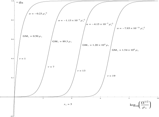
Figure 1: The positive branch. $\Omega(x)F(x)$ for a fixed horizon area. The horizontal axis is $\log_{10}(\sqrt{\Omega(x)}/\rho_{+}).$ This function is the analogue of the logarithm of the radial coordinate in the Schwarzschild geometry, normalized to be zero at the horizon.

The definition of the location of the horizon can be used to find the value of the parameter $\alpha$ in terms of $x_{+}$ and $\eta$ and $\nu$. Finally, $\eta$ and $\alpha$ can be replaced in the negative of the lapse function to obtain $F(x)\Omega(x)$ as a function of $x$, $x_{+}$ and $\nu$. These graphs are independent of $\rho_{+}$. They depend on $x_{+}$ through the relation of the Komar mass and $\rho_{+}$ and the relation of $\alpha$ and $\rho_{+}^{-2}$.

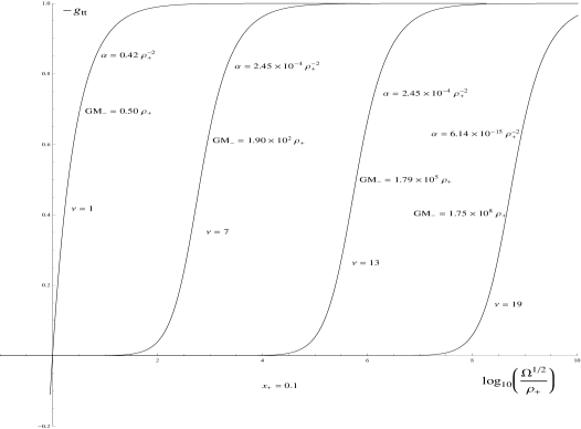
Figure 2: The negative branch. $\Omega(x)F(x)$ for a fixed horizon. The horizontal axis is $\log_{10}(\sqrt{\Omega(x)}/\rho_{+}).$This function is the analogue of the logarithm of the radial coordinate in the Schwarzschild geometry, normalized to be zero at the horizon.

The fact that the horizontal axis is on a logarithmic scale shows how flat can the gravitational field be made in the presence of the scalar field. This effect is a purely general relativistic effect. It is very interesting to note that the second derivative of the scalar field potential is zero at $\phi=0$, and therefore the scalar field is massless at infinity. However this massless scalar, due to the non-linear structure of the Einstein equations, has a strong effect in the gravitational field; it smoothly enhance the gravitational field from the Schwarzschild solution to large deviations from it.

6 The scalar field potential.

When $\Lambda=0$ the potential is odd, namely $V^{O}(\phi)=-V^{O}(-\phi)$. It follows that the stability of these solutions is an issue that should be addressed. While the actual calculation on the mechanical stability is a non-trival task, that will be addresed on a future work, this section shows that there are positive values of the cosmological constant that make the potential convex.

The more general potential (1), modifies the solution presented here in a simple way:

$$F^{\Lambda}(r)=F(r)-\frac{\Lambda}{3}.$$ (26)

To understand the structure of the potential when $\Lambda>0$, we note that, as follows from (1), the potential is even if $\alpha=\alpha_{E}\equiv\frac{\Lambda\left(\nu^{2}-4\right)}{6}$. In this case (1) takes the following form:

$$V^{\alpha=\alpha_{E}}(\phi)=\frac{\Lambda\left(\nu^{2}-4\right)}{6\kappa\nu^{2}}\left(\frac{\nu-1}{\nu+2}\cosh(\left(1+\nu\right)\phi l_{\nu})+\frac{\nu+1}{\nu-2}\cosh(\left(1-\nu\right)\phi l_{\nu})+4\frac{\nu^{2}-1}{\nu^{2}-4}\cosh\left(\phi l_{\nu}\right)\right).$$ (27)

From the form of the even potential it follows that its leading asymptotic form is:

$$V^{\alpha=\alpha_{E}}(\phi=\pm\infty)=\frac{\Lambda\left(\nu-2\right)\left(\nu-1\right)}{12\kappa\nu^{2}}\exp((\nu+1)\left|\phi\right|l_{\nu}).$$ (28)

More generally, the potential has the following asymptotic expansions for large values of $\phi$:

$$V(\phi =+\infty)=\frac{\alpha}{2\nu^{2}\kappa}\left(\frac{\nu-1}{\nu+2}\right)\exp(\left(1+\nu\right)\phi l_{\nu}),$$ (29)

$$V(\phi =-\infty)=\frac{1}{2\nu^{2}\kappa}\left(\frac{\nu-1}{\nu+2}\right)\left(-\alpha+\frac{\Lambda\left(\nu^{2}-4\right)}{3}\right)\exp(-\left(1+\nu\right)\phi l_{\nu}).$$ (30)

When $\alpha=0$ the leading behavior of the potential is:

$$V^{\alpha=0}(\phi=+\infty)=\frac{\Lambda\left(\nu+2\right)\left(\nu+1\right)}{6\kappa\nu^{2}}e^{\left(\nu-1\right)\phi l_{\nu}},\qquad V^{\alpha=0}(\phi=-\infty)=\frac{\Lambda\left(\nu-2\right)\left(\nu-1\right)}{6\kappa\nu^{2}}e^{-\left(\nu+1\right)\phi l_{\nu}}.$$ (31)

It can be noticed from (30) that when $\alpha=2\alpha_{E}=\frac{\Lambda\left(\nu^{2}-4\right)}{3}$ the leading behavior at infinity is also different. In fact, $V^{\alpha=0}(\phi)=V^{\alpha=2\alpha_{E}}(-\phi)$. It is possible to make a classification of all the possible behaviors of the potential for different values of $\Lambda$, $\nu$ and $\alpha$. This classification will be reported separatedly because it contains more than twenty different situations. The case that is more compelling in favor of the stability is:

When $\nu>2$ and $\frac{\Lambda\left(\nu^{2}-4\right)}{3}>\alpha>0$. The potential is positive for large values of $\left|\phi\right|$. The scalar field potential has a minimum at $\phi=0$.

The reparametrization of the solution in terms of $x_{+}$, $\rho_{+}$ and $\nu$ implies that:

$$\alpha=\frac{(\nu^{2}-4)\nu^{2}x_{+}^{\nu}(\Lambda\rho_{+}^{2}-3x_{+})}{3\rho_{+}^{2}\left(x_{+}^{\nu}\left(x_{+}^{\nu+2}\left(\nu-2\right)+x_{+}^{2}\left(4-\nu^{2}\right)+\nu^{2}\right)-x_{+}^{2}(\nu+2)\right)}.$$ (32)

It follows from this expression that all the cases of the negative branch of the previous section can satisfy $\frac{\Lambda\left(\nu^{2}-4\right)}{3}>\alpha>0$ for a range of positive values for $\Lambda$. These values can be made as small as required for small enough $x_{+}$.

7 Final Remarks.

Before this work there was only one uncharged, spherically symmetric black hole in four dimensional general relativity; now there is an infinite family of them. Inded, we make reference to configurations that are everywhere regular except at the usual Schwarzschild singularity.

As follows from the analysis of the lapse function, the scalar field allows to have much larger than Schwarzschild ammounts of mass in a given region of the spacetime. If this scalar field would actually exist, relatively small black holes can be much more massive than one would expect based on the Schwarzschild solution. These smaller but massive black holes strongly modify the universal law of gravity not only in its near surroundings but also in arbitrarily far regions from their location. It is tempting to conjecture that these geometries can be usefull to describe the geodesic motion of actual test particles in an astrophysical situation, like the well known flat galactic rotation curves. However, this can be considered as a serious posibility only after a study of the stability of these solutions is made. This, indeed, will be addressed in a future publication.

8 Acknowledgments.

We thank the useful coments of Nicolas Grandi about this work. Research of A.A. is supported in part by the Alexander von Humboldt foundation and by the Conicyt grant Anillo ACT-91: “Southern Theoretical Physics Laboratory” (STPLab). The work of J. O. was supported by FONDECYT grant 11090281.

References

- [1] J. D. Bekenstein, ‘No Hair’: Twenty–five Years After, chapter in Proceedings of the Second International Andrei D. Sakharov Conference in Physics, edited by I. M. Dremin and A. M. Semikhatov (World Scientific, Singapore, 1997).
- [2] M. Heusler, “A Mass bound for spherically symmetric black hole space-times,” Class. Quant. Grav. 12 (1995) 779 [gr-qc/9411054].
- [3] D. Sudarsky, “A Simple proof of a no hair theorem in Einstein Higgs theory,,” Class. Quant. Grav. 12 (1995) 579.
- [4] U. Nucamendi and M. Salgado, “Scalar hairy black holes and solitons in asymptotically flat space-times,” Phys. Rev. D 68 (2003) 044026 [gr-qc/0301062].
- [5] L. Sadeghian and C. M. Will, “Testing the black hole no-hair theorem at the galactic center: Perturbing effects of stars in the surrounding cluster,” Class. Quant. Grav. 28 (2011) 225029 [arXiv:1106.5056 [gr-qc]]. C. M. Will, “Testing the general relativistic no-hair theorems using the Galactic center black hole SgrA*,” arXiv:0711.1677 [astro-ph].
- [6] A. Anabalon, “Exact Black Holes and Universality in the Backreaction of non-linear Sigma Models with a potential in (A)dS4,” arXiv:1204.2720 [hep-th].
- [7] P. Amaro-Seoane, J. Barranco, A. Bernal and L. Rezzolla, “Constraining scalar fields with stellar kinematics and collisional dark matter,” JCAP 1011 (2010) 002 [arXiv:1009.0019 [astro-ph.CO]].
- [8] P. Amaro-Seoane, “Stellar dynamics and extreme-mass ratio inspirals,” arXiv:1205.5240 [astro-ph.CO].
- [9] M. Henneaux, C. Martinez, R. Troncoso and J. Zanelli, “Asymptotically anti-de Sitter spacetimes and scalar fields with a logarithmic branch,” Phys. Rev. D 70 (2004) 044034 [hep-th/0404236]. M. Henneaux, C. Martinez, R. Troncoso and J. Zanelli, “Asymptotic behavior and Hamiltonian analysis of anti-de Sitter gravity coupled to scalar fields,” Annals Phys. 322 (2007) 824 [hep-th/0603185].
- [10] C. Martínez, R. Troncoso, and J. Zanelli, “De Sitter black hole with a conformally coupled scalar field in four dimensions,” Phys. Rev. D 67, 024008 (2003) [arXiv:hep-th/0205319]. C. Martínez, J. P. Staforelli, and R. Troncoso, “Charged topological black hole with a conformally coupled scalar field,” Phys. Rev. D 74, 044028 (2006) [arXiv:hep-th/0512022]. E. Radu and E. Winstanley, “Conformally coupled scalar solitons and black holes with negative cosmological constant,” Phys. Rev. D 72, 024017 (2005) [arXiv:gr-qc/0503095]. A. Anabalon, H. Maeda, “New Charged Black Holes with Conformal Scalar Hair,” Phys. Rev. D81 (2010) 041501. [arXiv:0907.0219 [hep-th]]. C. Charmousis, T. Kolyvaris, and E. Papantonopoulos, “Charged C-metric with conformally coupled scalar field,” Class. Quant. Grav. 26, 175012 (2009) [arXiv:0906.5568 [gr-qc]]. T. Kolyvaris, G. Koutsoumbas, E. Papantonopoulos and G. Siopsis, “A New Class of Exact Hairy Black Hole Solutions,” Gen. Rel. Grav. 43 (2011) 163 [arXiv:0911.1711 [hep-th]]. M. J. Duff, J. T. Liu, “Anti-de Sitter black holes in gauged N = 8 supergravity,” Nucl. Phys. B554 (1999) 237-253. [hep-th/9901149]. T. Kolyvaris, G. Koutsoumbas, E. Papantonopoulos and G. Siopsis, “Einstein Hair,” arXiv:1111.0263 [gr-qc]. S. G. Saenz and C. Martinez, “Anti-de Sitter massless scalar field spacetimes in arbitrary dimensions,” arXiv:1203.4776 [hep-th]. A. Anabalon, F. Canfora, A. Giacomini and J. Oliva, “Black Holes with Primary Hair in gauged N=8 Supergravity,” arXiv:1203.6627 [hep-th]. A. Anabalon and A. Cisterna, “Asymptotically (anti) de Sitter Black Holes and Wormholes with a Self Interacting Scalar Field in Four Dimensions,” arXiv:1201.2008 [hep-th]. A. Anabalon and H. Maeda, “New Charged Black Holes with Conformal Scalar Hair,” Phys. Rev. D 81 (2010) 041501 [arXiv:0907.0219 [hep-th]]. A. Anabalon, F. Canfora, A. Giacomini and J. Oliva, “Black Holes with Primary Hair in gauged N=8 Supergravity,” arXiv:1203.6627 [hep-th]. Y. Bardoux, M. M. Caldarelli and C. Charmousis, “Conformally coupled scalar black holes admit a flat horizon due to axionic charge,” arXiv:1205.4025 [hep-th].
- [11] R. M. Wald, General Relativity, (University of Chicago Press, 1984), p.491.