A minimal model for the inelastic mechanics of biopolymer networks and cells

Abstract

Live cells have ambiguous mechanical properties. They were often described as either elastic solids or viscoelastic fluids and have recently been classified as soft glassy materials characterized by weak power-law rheology. Nonlinear rheological measurements have moreover revealed a pronounced inelastic response indicative of a competition between stiffening and softening. It is an intriguing question whether these observations can be explained from the material properties of much simpler in-vitro reconstituted networks of biopolymers that serve as reduced model systems for the cytoskeleton. Here, we explore the mechanism behind the inelastic response of cells and biopolymer networks, theoretically. Our analysis is based on the model of the inelastic glassy wormlike chain that accounts for the nonlinear polymer dynamics and transient crosslinking in biopolymer networks. It explains how inelastic and kinematic-hardening type behavior naturally emerges from the antagonistic mechanisms of viscoelastic stress-stiffening due to the polymers and inelastic fluidization due to bond breaking. It also suggests a simple set of schematic constitutive equations which faithfully reproduce the rich inelastic phenomenology of biopolymer networks and cells.

I Introduction

The mechanical properties of cells strongly influence processes in living organisms on all length scales, from the locomotion of single cells to the expansion of whole tissues during breathing. Therefore, studying the material properties of cells has a long tradition Pelling2008 . One of the major lessons learned so far is that cells are neither solid nor fluid, but can tune their mechanical state according to their needs. It is clear by now that this mechanical state is not simply predefined by biochemical processes, but that cells can be characterized as complex materials with nontrivial nonlinear mechanical feedback. Cell mechanics also couples back to the physiological response of cells Fletcher2010 , for example to the spreading behavior Pelham1997 or even to stem cell differentiation Discher2005 . In this contribution, we aim at elucidating the fundamental physics providing cells with their unique material properties. We make use of the fact that the mechanical response of the cell can be ascribed to the cytoskeleton Alberts2002 , a complex biopolymer network. Within the constituents of the cytoskeleton the dominant response is contributed by the actin cortex, a semiflexible polymer network connected by weak, reversible crosslinks. It is the microstructure of this actin cortex that we use as starting point for modeling. More precisely, we base our discussion on a model for transiently crosslinked biopolymer networks, called the inelastic glassy wormlike chain (inelastic Gwlc) Wolff2010 . From the inelastic Gwlc, which is numerically still quite demanding, we extract a reduced constitutive model that is more tractable both analytically and numerically. We restrict ourselves to reversible (“no-slip”) on-off kinetics, but find the model nevertheless capable of describing a large part of the known experimental data. For illustration, we evaluate the response to a standard deformation protocol.

II The inelastic Gwlc

The inelastic glassy wormlike chain (inelastic Gwlc) Wolff2010 is a phenomenological mean-field type model that describes a test polymer fluctuating against a background network. The slowing-down of the conformational dynamics of the test polymer by the surrounding network is phenomenologically represented by a stretching of its mode spectrum. More precisely, the single mode relaxation time $\tau_{n}$ of the $n$th eigenmode of a free polymer is modified according to

$$\tau_{n}\to\tilde{\tau}_{n}=\left\{\begin{array}[]{c c}\tau_{n}&\lambda_{n}<\Lambda\\ \tau_{n}\exp\left[\mathcal{E}(\lambda_{n}/\Lambda-1)\right]&\lambda_{n}\geq\Lambda\end{array}\right..$$ (1)

In the spirit of a mean-field model, $\mathcal{E}$ and $\Lambda$ are below interpreted as the characteristic free energy barrier of, and the average contour distance between, weak transient bonds, respectively, and $\lambda_{n}$ is the wavelength of the $n$th mode of the polymers’s transverse contour fluctuations $r_{\perp}(s,t)$. Inserting the modified relaxation spectrum, Eq. (1), into the expression for the mechanical response of an isolated wormlike chain in solution yields a highly successful phenomenological parametrization of the equilibrium response of sticky biopolymer networks Semmrich2007 and even of living cells Kroy2009 . For example, the susceptibility of a test polymer of bending rigidity $\kappa$ to a transverse point force is given by Kroy2007

$$\alpha(\omega)=\frac{\Lambda^{3}}{\kappa\pi^{4}}\int_{0}^{\infty}d\tilde{n}\frac{1}{(\tilde{n}^{4}+\tilde{n}^{2}f/f_{\Lambda})(1+i\omega\tilde{\tau}_{\tilde{n}})},$$ (2)

where $f_{\Lambda}$ is the Euler buckling force.

We found the above interpretation of the mathematical expression in terms of physical network parameters particularly useful for non-equilibrium processes, in which the bond network is driven out of equilibrium so that the average bond distance $\Lambda$ deviates from its force-free reference value $\Lambda_{0}$ according to

$$\frac{\Lambda}{\Lambda_{0}}=\frac{\nu_{0}}{\nu},$$ (3)

where $\nu$ quantifies the fraction of broken bonds and $\nu_{0}$ is the respective equilibrium value. For simplicity, we model $\nu$ by a first-order kinetic equation with two possible states, bound and unbound, characterized by on and off rates $k_{+}$ and $k_{-}$, respectively Wolff2010

$$\dot{\nu}(t,f)=-\left\{k_{+}(f)+k_{-}(f)\right\}\nu(t)+k_{+}(f).$$ (4)

The rates are prescribed by Kramers‘ theory Kramers1940 and an exponential force dependence according to Bell’s model Bell1978 , i.e. 

$$k_{+}(f)=ke^{U-\Delta x_{u}f},$$ (5)

and

$$k_{-}(f)=ke^{\Delta x_{b}f},$$ (6)

with $k\sim\tau_{0}^{-1}e^{-\mathcal{E}}$. They depend on the height $\mathcal{E}k_{\rm B}T$ of the the energy barrier separating bound and unbound state, the relative binding affinity $e^{U}$, and the widths $\Delta x_{b}$ and $\Delta x_{u}$ of the bound and unbound state, respectively. In the following, the thermal energy $k_{\rm B}T$ is set to one for convenience.

III Simplified constitutive equations

The crucial feature of the inelastic Gwlc is that the mutual interaction of the “stiff” polymer response and the “soft” bond network generates a huge variety of phenomena, depending on the particular stimulus. Here, we are interested in the long-time quasi-plastic response, and not in short-time effects and the particular shape of the relaxation spectrum, which we discussed elsewhere Wolff2010 . We therefore refrain from reproducing all the details of the full model and concentrate on those aspects that are most important in this respect, namely a nearly exponential strain stiffening and the softening due to the reversible breaking of weak bonds. This leads to a reduced simplified formulation of the inelastic Gwlc that allows for the analytical derivation of constitutive equations for transiently crosslinked biopolymer networks.

To arrive at these equations, we cast the model equations into a form that emphasizes common aspects of plasticity theory. As a starting point, the system size $L$ is related to the initial size $L_{0}$ by a scaling function $\alpha^{\rm nl}$ that characterizes the nonlinear compliance in terms of the dimensionless bond fraction $\nu$,

$$L=L_{0}\alpha^{\rm nl}\left[f,\nu(f)\right].$$ (7)

The inelastic Gwlc model predicts a monotonic decrease of the material stiffness with the bond fraction Wolff2010 , i.e. the more bonds are broken, the more susceptible the material becomes to deformations. For the sake of the argument, we approximate the precise functional form by a simple reciprocal dependence of the nonlinear susceptibility on the bond fraction,

$$\alpha^{\rm nl}\left[f,\nu(f)\right]\equiv\frac{\nu_{0}}{\nu}\delta(f,\nu_{0}).$$ (8)

Here, we have introduced the (nonlinearly) elastic component $\delta$. It only depends on the equilibrium bond fraction $\nu_{0}$ under zero external force, while the dependence on the current bond fraction $\nu$ is isolated into the prefactor. Defining the inelastic length $\mathcal{L}$ as the part of the extension that is not due to elastic deformations,

$$\mathcal{L}\equiv L_{0}\nu_{0}/\nu,$$ (9)

the actual system length can now be written as

$$L=\mathcal{L}\cdot\delta.$$ (10)

Stressing the similarities to plasticity theory, we can associate a “rest force” $\mathcal{F}$ with the inelastic length, defined by the condition $\mathcal{\dot{L}}=0$. Given our knowledge of the bond kinetics, the rest force is easily calculated. According to Eq. (9), $\mathcal{\dot{L}}=0\Leftrightarrow\dot{\nu}=0$. The rest force $\mathcal{F}$ is therefore determined by the following condition

$$\mathcal{F}:\dot{\nu}(t)|_{\mathcal{F}}=0.$$ (11)

By Eqs. (4)-(6), for a given force $f$, $\dot{\nu}=0\Leftrightarrow\nu=\left(1+e^{(\Delta x_{b}+\Delta x_{u})f-U}\right)^{-1}$, yielding

$$(\Delta x_{b}+\Delta x_{u})\mathcal{F}=U+\ln\left(\frac{\mathcal{L}}{L_{0}\nu_{0}}-1\right),$$ (12)

where we solved for f and replaced $\nu$ using relation (9). In the context of bond kinetics, $\mathcal{F}$ is the force that would have to be maintained to render the current bond fraction stationary. Taking a time derivate, the rest force is seen to inherit its dynamics from the inelastic deformation rate $\dot{\mathcal{L}}$, a phenomenon commonly denoted as kinematic hardening. However, in contrast to the common linear kinematic hardening ($\dot{\mathcal{F}}\propto\dot{\mathcal{L}}$), bond breaking leads to the phenomenology of logarithmic kinematic hardening, $\dot{\mathcal{F}}\propto\dot{\mathcal{L}}/\mathcal{L}$. Note that $\mathcal{F}$ is finite for ${\mathcal{L}}>L_{0}\nu_{0}$ and that, by definition, $\mathcal{F}=0$ for $\mathcal{L}=L_{0}$.

The corresponding flow rule can be found by decomposing the total mechanical force $f=\mathcal{F}+\Delta f$ into the rest force $\mathcal{F}$ and an overstress $\Delta f$, and inserting it into the force-dependent bond kinetics, Eqs. (4)-(6). Eliminating $\mathcal{F}$ using Eq. (12), and expressing the result in terms of the inelastic length $\mathcal{L}$, the flow rule is given by

$$e^{-\epsilon\cdot U}\cdot\tau_{0}e^{\mathcal{E}}\cdot\frac{\dot{\mathcal{L}}}{\mathcal{L}}\cdot\left(\frac{\mathcal{L}}{L_{0}\nu_{0}}-1\right)^{-\epsilon}=\left(e^{\Delta x_{b}\Delta f}-e^{-\Delta x_{u}\Delta f}\right),$$ (13)

where we introduced the abbreviation $\epsilon\equiv\Delta x_{b}/(\Delta x_{b}+\Delta x_{u})$. At any instant $t$, Eq. (13) uniquely determines $\mathcal{L}$, given the overstress history $\Delta f(t)$. Note that the equations derived above do not depend on the particular choice of the elastic response $\delta$.

To summarize this section, we found a set of constitutive equations from an approximate model based on the molecular structure of the cytoskeleton, describing the inelastic mechanical response of a transiently crosslinked biopolymer network. We can now proceed to evaluate the equations and to numerically examine the responses to a simple deformation protocol.

IV Quasi-plastic response

We consider the response of the model to a deformation ramp $\dot{\Gamma}\equiv\dot{L}/L_{0}=\dot{\Gamma}_{0}\equiv{\rm const.}$, followed by a plateau $\dot{\Gamma}=0$ and an inverse ramp, $\dot{\Gamma}=-\dot{\Gamma}_{0}$ (Fig. 1, lower panel, inset). The elastic contribution of the inelastic Gwlc is well approximated by exponential elasticity, $f(\delta)\propto(\delta-1)e^{\gamma\cdot(\delta-1)^{2}}$, which has been observed for a multitude of biomaterials Fung1993 . For simplicity, we also neglect the viscous component of the viscoelastic polymer response, as it is not essential for the following argumentation. The qualitative effects presented in the following do not depend on these technically motivated simplifications.

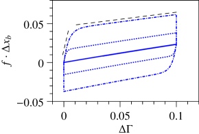
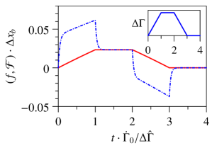
Figure 1: Response of the simplified schematic model for biopolymer networks, Eqs. (10)-(13), derived from the inelastic Gwlc, to a piece-wise linear deformation protocol (loading-waiting-unloading, see inset of lower panel). The relative deformation amplitude is $\Delta\hat{\Gamma}=10\%$, and ramp and plateau durations are $\Delta\hat{\Gamma}/\dot{\Gamma}_{0}$. Upper panel: force-displacement curves [deformation rates $\dot{\Gamma}_{0}\tau_{0}e^{\mathcal{E}}=$ 0.004 (solid lines), 0.64 (dotted lines), and 1.6 (dot-dashed lines)]; dashed lines indicating elastic and apparent kinematic hardening regimes, respectively, reminiscent of what is observed for living cells Fernandez2008 . Lower panel: time-dependent force for the highest deformation rate (dot-dashed lines) compared to the time-dependent rest force $\mathcal{F}$ (solid lines); forces are normalized by the natural force scale $\Delta x_{\rm b}^{-1}$ (in units of $k_{\rm B}T$) of the bound state.

The force-displacement curves exhibit rate-dependent hysteresis (Fig. 1, upper panel), which in our model is a signature of dissipation caused by inelastic reversible bond breaking. In the limit of an infinitely slow deformation, the bonds are always in equilibrium and the hysteresis vanishes (solid lines in the upper panel of Fig. 1), since we dismissed the viscoelastic hysteresis present in the Gwlc model and real biopolymer materials, here. For low to moderate rates (the time scale is set by the intrinsic time scale $\tau_{0}e^{\mathcal{E}}$ of the bonds), all force-displacement curves share characteristic features. Most prominently, the response to a linear ramp is characterized by two approximately linear regimes, emphasized by the dashed lines in the upper panel of Fig. 1. The first linear regime can be interpreted as an elastic response. The second regime is explained by a quasi-plastic deformation with slowly increasing rest force $\mathcal{F}$, a signature of the apparent kinematic hardening identified above [see Eq. (12)], where we found that the rest force depends logarithmically on the inelastic deformation, suggesting the notion of “logarithmic kinematic hardening”. Corresponding deviations from the linear force-displacement curve become discernible for deformations with amplitudes much larger than $10\%$ (not shown). The phenomenology is reminiscent of experimental results obtained for living cells Fernandez2008 .

The interpretation of an elastic and an inelastic regime is substantiated by comparing the time-dependent rest force $\mathcal{F}$ to the total mechanical force $f$ (Fig. 1, lower panel). While during a ramp, the total mechanical force initially strongly diverges from the rest force, it quickly settles on a course parallel to the rest force, consistent with a constant elastic contribution. The elastic contribution is relaxed upon halting the deformation. The force characterizing the transition between elastic and inelastic regime can be interpreted as an effective yield threshold. For infinitely slow deformations, the total mechanical force equals the rest force, and no predominantly elastic regime is present. In other words, also the effective yield threshold depends on the deformation rate. This observation sets our biopolymer network apart from usual models for hard solids. The reason for this behavior is that, by construction, the bonds will always yield if the stimulus is slow compared to the bond-opening time scale. Only for sufficiently fast deformation, an initial predominantly elastic response can be obtained.

V Conclusions

Starting from a minimal model of a transiently crosslinked biopolymer network, we derived quasi-plastic constitutive equations exhibiting logarithmic kinematic hardening. In contrast to “truly” plastic materials, the inelastic deformations are rooted in the inelastic, reversible softening due to the transient breaking of weak bonds, as presumed by the cell rheological model of the inelastic Gwlc.

From the perspective of biomechanics, the present work may lead to an intuitive understanding of the mechanical properties of biopolymer materials and cells. It also provides a simple but accurate model to simulate the large-scale behavior of the materials, e.g. using finite element methods. From the perspective of materials science, our work sheds light on a new class of materials, which can bear a kind of strain that is both recoverable and dissipative, as opposed to the “usual” reversible elastic and the irreversible plastic strain. This recoverable inelastic strain bears resemblance to the quasi-plastic-elastic (QPE) model recently proposed in relation with DP steel alloys Sun2011 . In contrast to the QPE strain, however, our recoverable inelastic strain is rate-dependent, due to the underlying slow bond dynamics. It is an intriguing question whether the QPE strain might emerge from the bond-breaking approach in some special limiting case. As an outlook, we would like to mention that it would be straightforward to extend our model to account for true plastic strains Fernandez2008 (by associating some slip with each bond breaking event) as well as for the physiologically important internally generated active stresses Wang2002 ; Stamenovic2004 .

- (1) A. E. Pelling and M. A. Horton, Pflügers Archiv : European journal of physiology 456, 3 (Apr. 2008), ISSN 0031-6768, http://www.ncbi.nlm.nih.gov/pubmed/18064487
- (2) D. A. Fletcher and R. D. Mullins, Nature 463, 485 (Jan. 2010), ISSN 1476-4687, http://www.ncbi.nlm.nih.gov/pubmed/20110992
- (3) R. J. Pelham and Y. L. Wang, Proceedings of the National Academy of Sciences of the United States of America 94, 13661 (Dec. 1997), ISSN 0027-8424, http://www.ncbi.nlm.nih.gov/pubmed/11536880
- (4) D. E. Discher, P. Janmey, and Y.-L. Wang, Science (New York, N.Y.) 310, 1139 (Nov. 2005), ISSN 1095-9203, http://www.ncbi.nlm.nih.gov/pubmed/16293750
- (5) B. Alberts, A. Johnson, J. Lewis, M. Reff, K. Roberts, and P. Walter, Molecular Biology of the Cell, 4th ed. (Garland Science, 2002)
- (6) L. Wolff, P. Fernandez, and K. Kroy, New Journal of Physics 12, 053024 (May 2010), ISSN 1367-2630, http://stacks.iop.org/1367-2630/12/i=5/a=053024?key=crossref.5c7f25e310%f89bc6d9fa12696fb7e701
- (7) C. Semmrich, T. Storz, J. Glaser, R. Merkel, A. R. Bausch, and K. Kroy, Proceedings of the National Academy of Sciences of the United States of America 104, 20199 (Dec. 2007), ISSN 1091-6490, http://www.pubmedcentral.nih.gov/articlerender.fcgi?artid=2154408&tool%=pmcentrez&rendertype=abstract
- (8) K. Kroy and J. Glaser, AIP Conference Proceedings 1151, 52 (2009), http://link.aip.org/link/?APCPCS/1151/52/1
- (9) K. Kroy and J. Glaser, New Journal of Physics 9, 416 (Nov. 2007), ISSN 1367-2630, r7
- (10) H. Kramers, Physica VII, 284 (1940), http://linkinghub.elsevier.com/retrieve/pii/S0031891440900982
- (11) G. Bell, Science 200, 618 (May 1978), ISSN 0036-8075, http://www.sciencemag.org/cgi/doi/10.1126/science.347575
- (12) Y. Fung, Biomechanics: Mechanical Properties of Living Tissues (Springer, 1993)
- (13) P. Fernández and A. Ott, Physical Review Letters 100, 238102 (Jun. 2008), ISSN 0031-9007, http://link.aps.org/doi/10.1103/PhysRevLett.100.238102
- (14) L. Sun and R. Wagoner, International Journal of Plasticity 27, 1126 (Jul. 2011), ISSN 07496419, http://linkinghub.elsevier.com/retrieve/pii/S0749641910001889
- (15) N. Wang, I. Tolic-Norrelykke, J. Chen, S. M. Mijailovich, J. P. Butler, J. J. Fredberg, and D. Stamenović, American Journal of Cell Physiology 282, 606 (2002), http://ajpcell.physiology.org/cgi/content/abstract/282/3/C606
- (16) D. Stamenovic, B. Suki, B. Fabry, N. Wang, and J. J. Fredberg, Journal of applied physiology (Bethesda, Md. : 1985) 96, 1600 (May 2004), ISSN 8750-7587, http://www.ncbi.nlm.nih.gov/pubmed/14707148