A Domain-Specific Compiler for
Linear Algebra Operations

Abstract

We present a prototypical linear algebra compiler that automatically exploits domain-specific knowledge to generate high-performance algorithms. The input to the compiler is a target equation together with knowledge of both the structure of the problem and the properties of the operands. The output is a variety of high-performance algorithms, and the corresponding source code, to solve the target equation. Our approach consists in the decomposition of the input equation into a sequence of library-supported kernels. Since in general such a decomposition is not unique, our compiler returns not one but a number of algorithms. The potential of the compiler is shown by means of its application to a challenging equation arising within the genome-wide association study. As a result, the compiler produces multiple “best” algorithms that outperform the best existing libraries.

1 Introduction

In the past 30 years, the development of linear algebra libraries has been tremendously successful, resulting in a variety of reliable and efficient computational kernels. Unfortunately these kernels are limited by a rigid interface that does not allow users to pass knowledge specific to the target problem. If available, such knowledge may lead to domain-specific algorithms that attain higher performance than any traditional library [1]. The difficulty does not lay so much in creating flexible interfaces, but in developing algorithms capable of taking advantage of the extra information.

In this paper, we present preliminary work on a linear algebra compiler, written in Mathematica, that automatically exploits application-specific knowledge to generate high-performance algorithms. The compiler takes as input a target equation and information on the structure and properties of the operands, and returns as output algorithms that exploit the given information. In the same way that a traditional compiler breaks the program into assembly instructions directly supported by the processor, attempting different types of optimization, our linear algebra compiler breaks a target operation down to library-supported kernels, and generates not one but a family of viable algorithms. The decomposition process undergone by our compiler closely replicates the thinking process of a human expert.

We show the potential of the compiler by means of a challenging operation arising in computational biology: the genome-wide association study (GWAS), an ubiquitous tool in the fields of genomics and medical genetics [2, 3, 4]. As part of GWAS, one has to solve the following equation

$$\left\{{\begin{aligned} b_{ij}&:=(X_{i}^{T}M_{j}^{-1}X_{i})^{-1}X_{i}^{T}M_{j}^{-1}y_{j}\\ M_{j}&:=h_{j}\Phi+(1-h_{j})I\end{aligned}}\right.\;{\begin{aligned} \text{ with }&1\leq i\leq m\\ \text{ and }&1\leq j\leq t,\end{aligned}}$$ (1)

where $X_{i}$, $M_{j}$, and $y_{j}$ are known quantities, and $b_{ij}$ is sought after. The size and properties of the operands are as follows: $b_{ij}\in\mathcal{R}^{p}$, $X_{i}\in\mathcal{R}^{n\times p}$ is full rank, $M_{j}\in\mathcal{R}^{n\times n}$ is symmetric positive definite (SPD), $y_{j}\in\mathcal{R}^{n}$, $\Phi\in\mathcal{R}^{n\times n}$, and $h_{j}\in\mathcal{R}$; $10^{3}\leq n\leq 10^{4}$, $1\leq p\leq 20$, $10^{6}\leq m\leq 10^{7}$, and $t$ is either $1$ or of the order of $10^{5}$.

At the core of GWAS lays a linear regression analysis with non-independent outcomes, carried out through the solution of a two-dimensional sequence of the Generalized Least-Squares problem (GLS)

$$b:=(X^{T}M^{-1}X)^{-1}X^{T}M^{-1}y.$$ (2)

While GLS may be directly solved, for instance, by MATLAB, or may be reduced to a form accepted by LAPACK [5], none of these solutions can exploit the specific structure pertaining to GWAS. The nature of the problem, a sequence of correlated GLSs, allows multiple ways to reuse computation. Also, different sizes of the input operands demand different algorithms to attain high performance in all possible scenarios. The application of our compiler to GWAS, Eq. 1, results in the automatic generation of dozens of algorithms, many of which outperform the current state of the art by a factor of four or more.

The paper is organized as follows. Related work is briefly described in Section 2. Sections 3 and 4 uncover the principles and mechanisms upon which the compiler is built. In Section 5 we carefully detail the automatic generation of multiple algorithms, and outline the code generation process. In Section 6 we report on the performance of the generated algorithms through numerical experiments. We draw conclusions in Section 7.

2 Related work

A number of research projects concentrate their efforts on domain-specific languages and compilers. Among them, the SPIRAL project [6] and the Tensor Contraction Engine (TCE) [7], focused on signal processing transforms and tensor contractions, respectively. As described throughout this paper, the main difference between our approach and SPIRAL is the inference of properties. Centered on general dense linear algebra operations, one of the goals of the FLAME project is the systematic generation of algorithms. The FLAME methodology, based on the partitioning of the operands and the automatic identification of loop-invariants [8, 9], has been successfully applied to a number of operations, originating hundreds of high-performance algorithms.

The approach described in this paper is orthogonal to FLAME. No partitioning of the operands takes place. Instead, the main idea is the mapping of operations onto high-performance kernels from available libraries, such as BLAS [10] and LAPACK.

3 The compiler principles

In this section we expose the human thinking process behind the generation of algorithms for a broad range of linear algebra equations. As an example, we derive an algorithm for the solution of the GLS problem, Eq. 2, as it would be done by an expert. Together with the derivation, we describe the rationale for every step of the algorithm. The exposed rationale highlights the key ideas on top of which we founded the design of our compiler.

Given Eq. 2, the first concern is the inverse operator applied to the expression $X^{T}M^{-1}X$. Since $X$ is not square, the inverse cannot be distributed over the product and the expression needs to be processed first. The attention falls then on $M^{-1}$. The inversion of a matrix is costly and not recommended for numerical reasons; therefore, since $M$ is a general matrix, we factor it. Given the structure of $M$ (SPD), we choose a Cholesky factorization, resulting in

$$LL^{T} =M$$

$$b: =(X^{T}(LL^{T})^{-1}X)^{-1}X^{T}(LL^{T})^{-1}y,$$ (3)

where $L$ is square and lower triangular. As $L$ is square, the inverse may now be distributed over the product $LL^{T}$, yielding $L^{-T}L^{-1}$. Next, we process $X^{T}L^{-T}L^{-1}X$; we observe that the quantity $L^{-1}X$ appears multiple times, and may be computed and reused to save computation:

$$W :=L^{-1}X$$

$$b :=(W^{T}W)^{-1}W^{T}L^{-1}y.$$ (4)

At this point, since $W$ is not square and the inverse cannot be distributed, there are two alternatives: 1) multiply out $W^{T}W$; or 2) factor $W$, for instance through a QR factorization. In this example, we choose the former:

$$S :=W^{T}W$$

$$b :=S^{-1}W^{T}L^{-1}y.$$ (5)

One can prove that $S$ is SPD, suggesting yet another factorization. We choose a Cholesky factorization and distribute the inverse over the product:

$$GG^{T} =S$$

$$b :=G^{-T}G^{-1}W^{T}L^{-1}y.$$ (6)

Now that all the remaining inverses are applied to triangular matrices, we are left with a series of products to compute the final result. Since all operands are matrices except the vector $y$, we compute Eq. 6 from right to left to minimize the number of flops. The final algorithm is shown in Alg. 1, together with the names of the corresponding BLAS and LAPACK building blocks.

Algorithm 1: Solution of the GLS problem as derived by a human expert

⬇

1 $LL^{T}=M$ (potrf)

2 $W:=L^{-1}X$ (trsm)

3 $S:=W^{T}W$ (syrk)

4 $GG^{T}=S$ (potrf)

5 $y:=L^{-1}y$ (trsv)

6 $b:=W^{T}y$ (gemv)

7 $b:=G^{-1}b$ (trsv)

8 $b:=G^{-T}b$ (trsv)

Three ideas stand out as the guiding principles for the thinking process:

• The first concern is to deal, whenever it is not applied to diagonal or triangular matrices, with the inverse operator. Two scenarios may arise: a) it is applied to a single operand, $A^{-1}$. In this case the operand is factored with a suitable factorization according to its structure; b) the inverse is applied to an expression. This case is handled by either computing the expression and reducing it to the first case, or factoring one of the matrices and analyzing the resulting scenario.

• When decomposing the equation, we give priority to a) common segments, i.e., common subexpressions, and b) segments that minimize the number of flops; this way we reduce the amount of computation performed.

• If multiple alternatives leading to viable algorithms arise, we explore all of them.

4 Compiler overview

Our compiler follows the above guiding principles to closely replicate the thinking process of a human expert. To support the application of these principles, the compiler incorporates a number of modules ranging from basic matrix algebra support to analysis of dependencies, including the identification of building blocks offered by available libraries. In the following, we describe the core modules.

Matrix algebra

The compiler is written using Mathematica from scratch. We implement our own operators: addition (plus), negation (minus), multiplication (times), inversion (inv), and transposition (trans). Together with the operators, we define their precedence and properties, as commutativity, to support matrices as well as vectors and scalars. We also define a set of rewrite rules according to matrix algebra properties to freely manipulate expressions and simplify them, allowing the compiler to work on multiple equivalent representations.

Inference of properties

In this module we define the set of supported matrix properties. As of now: identity, diagonal, triangular, symmetric, symmetric positive definite, and orthogonal. On top of these properties, we build an inference engine that, given the properties of the operands, is able to infer properties of complex expressions. This module is extensible and facilitates incorporating additional properties.

Building blocks interface

This module contains an extensive list of patterns associated with the desired building blocks onto which the algorithms will be mapped. It also contains the corresponding cost functions to be used to construct the cost analysis of the generated algorithms. As with the properties module, if a new library is to be used, the list of accepted building blocks can be easily extended.

Analysis of dependencies

When considering a sequence of problems, as in GWAS, this module analyzes the dependencies among operations and between operations and the dimensions of the sequence. Through this analysis, the compiler rearranges the operations in the algorithm, reducing redundant computations.

Code generation

In addition to the automatic generation of algorithms, the compiler includes a module to translate such algorithms into code. So far, we support the generation of MATLAB code for one instance as well as sequences of problems.

To complete the overview of our compiler, we provide a high-level description of the compiler’s reasoning. The main idea is to build a tree in which the root node contains the initial target equation; each edge is labeled with a building block; and each node contains intermediate equations yet to be mapped. The compiler progresses in a breadth-first fashion until all leaf nodes contain an expression directly mapped onto a building block.

While processing a node’s equation, the search space is constrained according to the following criteria:

1. if the expression contains an inverse applied to a single (non-diagonal, non-triangular) matrix, for instance $M^{-1}$, then the compiler identifies a set of viable factorizations for $M$ based on its properties and structure;

2. if the expression contains an inverse applied to a sub-expression, for instance $(W^{T}W)^{-1}$, then the compiler identifies both viable factorizations for the operands in the sub-expression (e.g., $QR=W$), and segments of the sub-expression that are directly mapped onto a building block (e.g., $S:=W^{T}W$);

3. if the expression contains no inverse to process (as in $G^{-T}G^{-1}W^{T}L^{-1}y$, with $G$ and $L$ triangular), then the compiler identifies segments with a mapping onto a building block.

When inspecting expressions for segments, the compiler gives priority to common segments and segments that minimize the number of flops.

All three cases may yield multiple building blocks. For each building block —either a factorization or a segment— both a new edge and a new children node are created. The edge is labeled with the corresponding building block, and the node contains the new resulting expression. For instance, the analysis of Eq. 4 creates the following sub-tree:

In addition, thanks to the Inference of properties module, for each building block, properties of the output operands are inferred from those of the input operands.

Each path from the root node to a leaf represents one algorithm to solve the target equation. By assembling the building blocks attached to each edge in the path, the compiler returns a collection of algorithms, one per leaf.

Our compiler has been successfully applied to equations such as pseudo-inverses, least-squares-like problems, and the automatic differentiation of BLAS and LAPACK operations. Of special interest are the scenarios in which sequences of such problems arise; for instance, the study case presented in this paper, genome-wide association studies, which consist of a two-dimensional sequence of correlated GLS problems.

The compiler is still in its early stages and the code is not yet available for a general release. However, we include along the paper details on the input and output of the system, as well as screenshots of the actual working prototype.

5 Compiler-generated algorithms

We detail now the application to GWAS of the process described above. Box 1 includes the input to the compiler: the target equation along with domain-specific knowledge arising from GWAS, e.g, operands’ shape and properties. As a result, dozens of algorithms are automatically generated; we report on three selected ones.

equation = {
   equal[b,
      times[
         inv[times[
               trans[X],
               inv[plus[ times[h, Phi], times[plus[1, minus[h]], id] ]],
               X]
         ],
         trans[X],
         inv[plus[ times[h, Phi], times[plus[1, minus[h]], id] ]],
         y
      ]
   ]
};

operandProperties = {
   {X,   {‘‘Input’’,  ‘‘Matrix’’, ‘‘FullRank’’} },
   {y,   {‘‘Input’’,  ‘‘Vector’’ } },
   {Phi, {‘‘Input’’,  ‘‘Matrix’’, ‘‘Symmetric’’} },
   {h,   {‘‘Input’’,  ‘‘Scalar’’ } },
   {b,   {‘‘Output’’, ‘‘Vector’’ } }
};

expressionProperties = {
   inv[plus[ times[h, Phi], times[plus[1, minus[h]], id] ]], ‘‘SPD’’ };

sizeAssumptions = { rows[X] > cols[X] };

Box 1 Mathematica input to the compiler.

5.1 Algorithm 1

To ease the reader, we describe the process towards the generation of an algorithm similar to Alg. 1. The starting point is Eq. 1. Since $X$ is not square, the inverse operator applied to $X^{T}(h\Phi+(1-h)I)^{-1}X$ cannot be distributed over the product; thus, the inner-most inverse is $(h\Phi+(1-h)I)^{-1}$. The inverse is applied to an expression, which is inspected for viable factorizations and segments. Among the identified alternatives are a) the factorization of the operand $\Phi$ according to its properties, and b) the computation of the expression $h\Phi+(1-h)I$. Here we concentrate on the second case. The segment $h\Phi+(1-h)I$ is matched as the scal-add building block (scaling and addition of matrices); the operation is made explicit and replaced:

$$M :=h\Phi+(1-h)I$$

$$b :=(X^{T}M^{-1}X)^{-1}X^{T}M^{-1}y.$$ (7)

Now, the inner-most inverse is applied to a single operand, $M$, and the compiler decides to factor it using multiple alternatives: Cholesky ($LL^{T}=M$), QR ($QR=M$), eigendecomposition ($ZWZ^{T}=M$), and SVD ($U\Sigma V^{T}=M$). All the alternatives are explored; we focus now on the Cholesky factorization (potrf routine from LAPACK):

$$LL^{T} =M$$

$$b: =(X^{T}L^{-T}L^{-1}X)^{-1}X^{T}L^{-T}L^{-1}y.$$ (8)

After $M$ is factored and replaced by $LL^{T}$, the inference engine propagates a number of properties to $L$ based on the properties of $M$ and the factorization applied. Concretely, $L$ is square, triangular and full-rank.

Next, since $L$ is triangular, the inner-most inverse to be processed in Eq. 8 is $(X^{T}L^{-T}L^{-1}X)^{-1}$. In this case two routes are explored: either factor $X$ ($L$ is triangular and does not need further factorization), or map a segment of the expression onto a building block. We consider this second alternative. The compiler identifies the solution of a triangular system (trsm routine from BLAS) as a common segment appearing three times in Eq. 8, makes it explicit, and replaces it:

$$W :=L^{-1}X$$

$$b :=(W^{T}W)^{-1}W^{T}L^{-1}y.$$ (9)

Since $L$ is square and full-rank, and X is also full-rank, $W$ inherits the shape of $X$ and is labelled as full-rank. As $W$ is not square, the inverse cannot be distributed over the product yet. Therefore, the compiler faces again two alternatives: either factoring $W$ or multiplying $W^{T}W$. We proceed describing the latter scenario while the former is analyzed in Sec. 5.2. $W^{T}W$ is identified as a building block (syrk routine of BLAS), and made explicit:

$$S :=W^{T}W$$

$$b :=S^{-1}W^{T}L^{-1}y.$$ (10)

The inference engine plays an important role deducing properties of $S$. During the previous steps, the engine has inferred that $W$ is full-rank and rows[W] > cols[W]; therefore the following rule states that $W$ is SPD.

isSPDQ[ times[ trans[ A_?isFullRankQ ], A_ ] /; rows[A] > cols[A]
  := True;

This knowledge is now used to determine possible factorizations for $S$. We concentrate on the Cholesky factorization:

$$GG^{T} =S$$

$$b :=G^{-T}G^{-1}W^{T}L^{-1}y.$$ (11)

In Eq. 11, all inverses are applied to triangular matrices; therefore, no more treatment of inverses is needed. The compiler proceeds with the final decomposition of the remaining series of products. Since at every step the inference engine keeps track of the properties of the operands in the original equation as well as the intermediate temporary quantities, it knows that every operand in Eq. 11 are matrices except for the vector $y$. This knowledge is used to give matrix-vector products priority over matrix-matrix products, and Eq. 11 is decomposed accordingly. In case the compiler cannot find applicable heuristics to lead the decomposition, it explores the multiple viable mappings onto building blocks. The resulting algorithm, and the corresponding output from Mathematica, are assembled in Alg. 2, chol-gwas.

Algorithm 2: chol-gwas

⬇

1 $M:=h\Phi+(1-h)I$ (scal-add)

2 $LL^{T}=M$ (potrf)

3 $W:=L^{-1}X$ (trsm)

4 $S:=W^{T}W$ (syrk)

5 $GG^{T}=S$ (potrf)

6 $y:=L^{-1}y$ (trsv)

7 $b:=W^{T}y$ (gemv)

8 $b:=G^{-1}b$ (trsv)

9 $b:=G^{-T}b$ (trsv)

5.2 Algorithm 2

In this subsection we display the capability of the compiler to analyze alternative paths, leading to multiple viable algorithms. At the same time, we expose more examples of algebraic manipulation carried out by the compiler. The presented algorithm results from the alternative path arising in Eq. 10, the factorization of $W$. Since $W$ is a full-rank column panel, the compiler analyzes the scenario where $W$ is factored using a QR factorization (geqrf routine in LAPACK):

$$QR :=W$$

$$b :=((QR)^{T}QR)^{-1}(QR)^{T}L^{-1}y.$$ (12)

At this point, the compiler exploits the capabilities of the Matrix algebra module to perform a series of simplifications:

$$b :=((QR)^{T}QR)^{-1}(QR)^{T}L^{-1}y;$$

$$b :=(R^{T}Q^{T}QR)^{-1}R^{T}Q^{T}L^{-1}y;$$

$$b :=(R^{T}R)^{-1}R^{T}Q^{T}L^{-1}y;$$

$$b :=R^{-1}R^{-T}R^{T}Q^{T}L^{-1}y;$$

$$b :=R^{-1}Q^{T}L^{-1}y.$$ (13)

First, it distributes the transpose operator over the product. Then, it applies the rule

        times[ trans[ q_?isOrthonormalQ, q_ ] -> id,

included as part of the knowledge-base of the module. The rule states that the product $Q^{T}Q$, when $Q$ is orthogonal with normalized columns, may be rewritten (->) as the identity matrix. Next, since $R$ is square, the inverse is distributed over the product. More mathematical knowledge allows the compiler to rewrite the product $R^{-T}R^{T}$ as the identity.

In Eq. 13, the compiler does not need to process any more inverses; hence, the last step is to decompose the remaining computation into a sequence of products. Once more, $y$ is the only non-matrix operand. Accordingly, the compiler decomposes the equation from right to left. The final algorithm is put together in Alg. 3, qr-gwas.

Algorithm 3: qr-gwas

⬇

1 $M:=h\Phi+(1-h)I$ (scal-add)

2 $LL^{T}$ = $M$ (potrf)

3 $W$ := $L^{-1}X$ (trsm)

4 $QR=W$ (geqrf)

5 $y$ := $L^{-1}y$ (trsv)

6 $b$ := $Q^{T}y$ (gemv)

7 $b$ := $R^{-1}b$ (trsv)

5.3 Algorithm 3

This third algorithm exploits further knowledge from GWAS, concretely the structure of $M$, in a manner that may be overlooked even by human experts.

Again, the starting point is Eq. 1. The inner-most inverse is $(h\Phi+(1-h)I)^{-1}$. Instead of multiplying out the expression within the inverse operator, we now describe the alternative path also explored by the compiler: factoring one of the matrices in the expression. We concentrate in the case where an eigendecomposition of $\Phi$ (syevd or syevr from LAPACK) is chosen:

$$ZWZ^{T} =\Phi$$

$$b :=(X^{T}(hZWZ^{T}+(1-h)I)^{-1}X)^{-1}$$

$$\quad\quad X^{T}(hZWZ^{T}+(1-h)I)^{-1}y$$ (14)

where $Z$ is a square, orthogonal matrix with normalized columns, and $W$ is a square, diagonal matrix.

In this scenario, the Matrix algebra module is essential; it allows the compiler to work with alternative representations of Eq. 14. We already illustrated an example where the product $Q^{T}Q$, $Q$ orthonormal, is replaced with the identity matrix. The freedom gained when defining its own operators, allows the compiler to perform also the opposite transformation:

       id -> times[ Q, trans[ Q ] ];
       id -> times[ trans[ Q ], Q ];

To apply these rules, the compiler inspects the expression $hZWZ^{T}+(1-h)I$ for orthonormal matrices: $Z$ is found to be orthonormal and used instead of $Q$ in the right-hand side of the previous rules. The resulting expression is

$$b :=(X^{T}(hZWZ^{T}+(1-h)ZZ^{T})^{-1}X)^{-1}$$

$$\quad\quad X^{T}(hZWZ^{T}+(1-h)ZZ^{T})^{-1}y.$$ (15)

The algebraic manipulation capabilities of the compiler lead to the derivation of further multiple equivalent representations of Eq. 15. We recall that, although we focus on a concrete branch of the derivation, the compiler analyzes the many alternatives. In the branch under study, the quantities $Z$ and $Z^{T}$ are grouped on the left- and right-hand sides of the inverse, respectively:

$$(X^{T}(Z(hW+(1-h)I)Z^{T})^{-1}X)^{-1};$$

then, since both $Z$ and $hW+(1-h)I$ are square, the inverse is distributed:

$$(X^{T}(Z^{-T}(hW+(1-h)I)^{-1}Z^{-1})X)^{-1};$$

finally, by means of the rules:

        inv[ q_?isOrthonormalQ ] -> trans[ q ];
        inv[ trans[ q_?isOrthonormalQ ] ] -> q;

which state that the inverse of an orthonormal matrix is its transpose, the expression becomes:

$$(X^{T}Z(hW+(1-h)I)^{-1}Z^{T}X)^{-1}.$$

The resulting equation is

$$b :=(X^{T}Z(hW+(1-h)I)^{-1}Z^{T}X)^{-1}$$

$$\quad\quad X^{T}Z(hW+(1-h)I)^{-1}Z^{T}y.$$ (16)

The inner-most inverse in Eq. 16 is applied to a diagonal object ($W$ is diagonal and $h$ a scalar). No more factorizations are needed, $hW+(1-h)I$ is identified as a scal-add building block, and exposed:

$$D :=hW+(1-h)I$$

$$b :=(X^{T}ZD^{-1}Z^{T}X)^{-1}X^{T}ZD^{-1}Z^{T}y.$$ (17)

$D$ is a diagonal matrix; hence only the inverse applied to $X^{T}ZD^{-1}Z^{T}X$ remains to be processed. Among the alternative steps, we consider the mapping of the common segment $X^{T}Z$, that appears three times, onto the gemm building block (matrix-matrix product):

$$K :=X^{T}Z$$

$$b :=(KD^{-1}K^{T})^{-1}KD^{-1}Z^{T}y.$$ (18)

From this point on, the compiler proceeds as shown for the previous examples, and obtains, among others, Alg. 4, eig-gwas.

Algorithm 4: eig-gwas

⬇

1 $ZWZ^{T}$ = $\Phi$ (syevx)

2 $D:=hW+(1-h)I$ (add-scal)

3 $K:=X^{T}Z$ (gemm)

4 $V:=KD^{-1}$ (scal)

5 $S$ := $VK^{T}$ (gemm)

6 $QR$ = $S$ (geqrf)

7 $y:=Z^{T}y$ (gemv)

8 $b:=Vy$ (gemv)

9 $b:=Q^{T}b$ (gemv)

10 $b:=R^{-1}b$ (trsv)

At first sight, Alg. 4 might seem to be a suboptimal approach. However, as we show in Sec. 6, it is representative of a family of algorithms that play a crucial role when solving a certain sequence of GLS problems within GWAS.

5.4 Cost analysis

We have illustrated how our compiler, closely replicating the reasoning of a human expert, automatically generates algorithms for the solution of a single GLS problem. As shown in Eq. 1, in practice one has to solve one-dimensional ($t=1$) or two-dimensional ($t\approx 10^{5}$) sequences of such problems. In this context we have developed a module that performs a loop dependence analysis to identify loop-independent operations and reduce redundant computations. For space reasons, we do not further describe the module, and limit to the automatically generated cost analysis.

The list of patterns for the identification of building blocks included in the Building blocks interface module also incorporates the corresponding computational cost associated to the operations. Given a generated algorithm, the compiler composes the cost of the algorithm by combining the number of floating point operations performed by the individual building blocks, taking into account the loops over the problem dimensions.

Table 1 includes the cost of the three presented algorithms, which attained the lowest complexities for one- and two-dimensional sequences. While qr-gwas and chol-gwas share the same cost for both types of sequences, suggesting a very similar behavior in practice, the cost of eig-gwas differs in both cases. For the one-dimensional sequence the cost of eig-gwas is not only greater in theory, the practical constants associated to its terms increase the gap. On the contrary, for the two-dimensional sequence, the cost of eig-gwas is lower than the cost of the other two. This analysis suggests that qr-gwas and chol-gwas are better suited for the one-dimensional case, while eig-gwas is better suited for the two-dimensional one. In Sec. 6 we confirm these predictions through experimental results.

Scenario	yqr-gwasy	ychol-gwasy	yeig-gwasy
One instance	$O(n^{3})$	$O(n^{3})$	$O(n^{3})$
1D sequence	$O(n^{3}+mpn^{2})$	$O(n^{3}+mpn^{2})$	$O(n^{3}+mpn^{2}+mp^{2}n)$
2D sequence	$O(tn^{3}+mtpn^{2})$	$O(tn^{3}+mtpn^{2})$	$O(n^{3}+mpn^{2}+mtp^{2}n)$

Table 1: Computational cost for the three algorithms selected by the compiler.

5.5 Code generation

The translation from algorithms to code is not a straightforward task; in fact, when manually performed, it is tedious and error prone. To overcome this difficulty, we incorporate in our compiler a module for the automatic generation of code. As of now, we support MATLAB; an extension to Fortran, a much more challenging target language, is planned. We provide here a short overview of this module.

Given an algorithm as derived by the compiler, the code generator builds an abstract syntax tree (AST) mirroring the structure of the algorithm. Then, for each node in the AST, the module generates the corresponding code statements. Specifically, for the nodes corresponding to for loops, the module not only generates a for statement but also the specific statements to extract subparts of the operands according to their dimensionality; as for the nodes representing the building blocks, the generator must map the operation to the specific MATLAB routine or matrix expression. As an example of automatically generated code, the MATLAB routine corresponding to the aforementioned eig-gwas algorithm for a two-dimensional sequence is illustrated in Fig. 1.

Figure 1: MATLAB code corresponding to eig-gwas.

6 Performance experiments

We turn now the attention to numerical results. In the experiments, we compare the algorithms automatically generated by our compiler with LAPACK and GenABEL [11], a widely used package for GWAS-like problems. For details on GenABEL’s algorithm for GWAS, gwfgls, we refer the reader to [12]. We present results for the two most representative scenarios in GWAS: one-dimensional ($t=1$), and two-dimensional ($t>1$) sequences of GLS problems.

The experiments were performed on an 12-core Intel Xeon X5675 processor running at 3.06 GHz, with 96GB of memory. The algorithms were implemented in C, and linked to the multi-threaded GotoBLAS and the reference LAPACK libraries. The experiments were executed using 12 threads.

We first study the scenario $t=1$. We compare the performance of qr-gwas and chol-gwas, with GenABEL’s gwfgls, and gels-gwas, based on LAPACK’s gels routine. The results are displayed in Fig. 2. As expected, qr-gwas and chol-gwas attain the same performance and overlap. Most interestingly, our algorithms clearly outperform gels-gwas and gwfgls, obtaining speedups of 4 and 8, respectively.

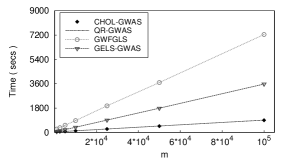
Figure 2: Timings for a one-dimensional sequence of GLS problems within GWAS. Problem sizes: $n=10{,}000$, $p=4$, $t=1$. The improvement in the performance of our algorithms is due to a careful exploitation of both the properties of the operands and the sequence of GLS problems.

Next, we present an even more interesting result. The current approach of all state-of-the-art libraries to the case $t>1$ is to repeat the experiment $t$ times with the same algorithm used for $t=1$. On the contrary, our compiler generates the algorithm eig-gwas, which particularly suits such scenario. As Fig. 3 illustrates, eig-gwas outperforms the best algorithm for the case $t=1$, chol-gwas, by a factor of 4, and therefore outperforms gels-gwas and gwfgls by a factor of 16 and 32 respectively.

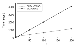
Figure 3: Timings for a two-dimensional sequence of GLS problems within GWAS. Problem sizes: $n=5{,}000$, $p=4$, $m=10^{6}$. chol-gwas is best suited for the scenario $t=1$, while eig-gwas is best suited for the scenario $t>>1$.

The results remark two significant facts: 1) the exploitation of domain-specific knowledge may lead to improvements in state-of-the-art algorithms; and 2) the library user may benefit from the existence of multiple algorithms, each matching a given scenario better than the others. In the case of GWAS our compiler achieves both, enabling computational biologists to target larger experiments while reducing the execution time.

7 Conclusions

We presented a linear algebra compiler that automatically exploits domain-specific knowledge to generate high-performance algorithms. Our linear algebra compiler mimics the reasoning of a human expert to, similar to a traditional compiler, decompose a target equation into a sequence of library-supported building blocks.

The compiler builds on a number of modules to support the replication of human reasoning. Among them, the Matrix algebra module, which enables the compiler to freely manipulate and simplify algebraic expressions, and the Properties inference module, which is able to infer properties of complex expressions from the properties of the operands.

The potential of the compiler is shown by means of its application to the challenging genome-wide association study equation. Several of the dozens of algorithms produced by our compiler, when compared to state-of-the-art ones, obtain n-fold speedups.

As future work we plan an extension to the Code generation module to support Fortran. Also, the asymptotic operation count is only a preliminary approach to estimate the performance of the generated algorithms. There is the need for a more robust metric to suggest a “best” algorithm for a given scenario.

8 Acknowledgements

The authors gratefully acknowledge the support received from the Deutsche Forschungsgemeinschaft (German Research Association) through grant GSC 111.

References

- [1] Bientinesi, P., Eijkhout, V., Kim, K., Kurtz, J., van de Geijn, R.: Sparse direct factorizations through unassembled hyper-matrices. Computer Methods in Applied Mechanics and Engineering 199 (2010) 430–438
- [2] Lauc, G., et al.: Genomics Meets Glycomics–The First GWAS Study of Human N-Glycome Identifies HNF1 as a Master Regulator of Plasma Protein Fucosylation. PLoS Genetics 6(12) (12 2010) e1001256
- [3] Levy, D., et al.: Genome-wide association study of blood pressure and hypertension. Nature Genetics 41(6) (Jun 2009) 677–687
- [4] Speliotes, E.K., et al.: Association analyses of 249,796 individuals reveal 18 new loci associated with body mass index. Nature Genetics 42(11) (Nov 2010) 937–948
- [5] Anderson, E., Bai, Z., Bischof, C., Blackford, S., Demmel, J., Dongarra, J., Du Croz, J., Greenbaum, A., Hammarling, S., McKenney, A., Sorensen, D.: LAPACK Users’ Guide. Third edn. Society for Industrial and Applied Mathematics, Philadelphia, PA (1999)
- [6] Püschel, M., Moura, J.M.F., Johnson, J., Padua, D., Veloso, M., Singer, B., Xiong, J., Franchetti, F., Gacic, A., Voronenko, Y., Chen, K., Johnson, R.W., Rizzolo, N.: SPIRAL: Code generation for DSP transforms. Proceedings of the IEEE, special issue on “Program Generation, Optimization, and Adaptation” 93(2) (2005) 232– 275
- [7] Baumgartner, G., Auer, A., Bernholdt, D.E., Bibireata, A., Choppella, V., Cociorva, D., Gao, X., Harrison, R.J., Hirata, S., Krishnamoorthy, S., Krishnan, S., chung Lam, C., Lu, Q., Nooijen, M., Pitzer, R.M., Ramanujam, J., Sadayappan, P., Sibiryakov, A., Bernholdt, D.E., Bibireata, A., Cociorva, D., Gao, X., Krishnamoorthy, S., Krishnan, S.: Synthesis of high-performance parallel programs for a class of ab initio quantum chemistry models. In: Proceedings of the IEEE. (2005) 2005
- [8] Fabregat-Traver, D., Bientinesi, P.: Knowledge-based automatic generation of partitioned matrix expressions. In Gerdt, V., Koepf, W., Mayr, E., Vorozhtsov, E., eds.: Computer Algebra in Scientific Computing. Volume 6885 of Lecture Notes in Computer Science., Springer Berlin / Heidelberg (2011) 144–157
- [9] Fabregat-Traver, D., Bientinesi, P.: Automatic generation of loop-invariants for matrix operations. In: Computational Science and its Applications, International Conference, Los Alamitos, CA, USA, IEEE Computer Society (2011) 82–92
- [10] Dongarra, J., Croz, J.D., Hammarling, S., Duff, I.S.: A set of level 3 basic linear algebra subprograms. ACM Trans. Math. Softw. 16(1) (1990) 1–17
- [11] Aulchenko, Y.S., Ripke, S., Isaacs, A., van Duijn, C.M.: Genabel: an R library for genome-wide association analysis. Bioinformatics 23(10) (May 2007) 1294–6
- [12] Fabregat-Traver, D., Aulchenko, Y.S., Bientinesi, P.: Fast and scalable algorithms for genome studies. Technical report, Aachen Institute for Advanced Study in Computational Engineering Science (2012) Available at http://www.aices.rwth-aachen.de:8080/aices/preprint/documents/AICES-2012-05-01.pdf.