Ghost propagator and the Coulomb form factor from the lattice

Abstract

We calculate the Coulomb ghost propagator $G(|\mathbf{p}|)$ and the static Coulomb potential $V_{C}(|\mathbf{r}|)$ for $SU(2)$ Yang-Mills theory on the lattice. In view of possible scaling violations related to deviations from the Hamiltonian limit we use anisotropic lattices to improve the temporal resolution. We find that the ghost propagator is infrared enhanced with an exponent $\kappa_{\rm gh}\gtrsim 0.5$ while the Coulomb potential exhibits a string tension larger than the Wilson string tension, $\sigma_{C}\simeq 2\sigma$. This agrees with the Coulomb “scaling” scenario derived from the Gribov-Zwanziger confinement mechanism.

I Introduction

Yang-Mills theories in Coulomb gauge have attracted increasing interest in the last years, both in the continuum and on the lattice. Non-perturbative analytic predictions based on the Gribov-Zwanziger confinement mechanism Gribov (1978); Zwanziger (1997) turn out to be concise and elegant in this gauge and numerical simulations have confirmed them so far.

In covariant gauges the Gribov-Zwanziger approach requires a restriction of the functional integral beyond the Faddeev-Popov mechanism Faddeev and Popov (1967), which has long been known to be insufficient to extract a unique field representative along the gauge orbit and thus cannot be used to define the partition function beyond perturbation theory Gribov (1978); Singer (1978); Killingback (1984). As a remedy one adds extra terms to the action which are, in general, non-local and often referred to as the Horizon function or Horizon condition. The purpose of these extra terms is to limit the fields in the functional integral to the so-called fundamental modular region $\Lambda$, which contains only absolute minima of the gauge fixing functional and thus eliminates the over-counting of gauge copies from the same orbit (except for topologically non-trivial copies).

In practice, however, it is almost impossible to limit the functional integral beyond the so-called first Gribov region $\Omega\supseteq\Lambda$, where the Faddeev-Popov operator is positive definite. Moreover, any restriction on the integration range imposed other than through the Faddeev-Popov mechanism will break the Becchi-Rouet-Stora-Tyutin (BRST) symmetry Becchi et al. (1976); Tyutin (1975). Whether such enlarged action including Horizon terms exhibits some other symmetry and what the possible consequences in covariant gauges are (e.g. in terms of contributions from non-standard condensates Burgio et al. (1998); Akhoury and Zakharov (1998); Boucaud et al. (2000); Dudal et al. (2010)) is still under active debate, cfr. Ref. Vandersickel and Zwanziger (2012); Dudal and Sorella (2012) and references therein for recent results.

In contrast to the situation in covariant gauges sketched above, the physical implications of the Gribov-Zwanziger approach are quite transparent in Coulomb gauge. In the Hamiltonian formulation Christ and Lee (1980); Szczepaniak and Swanson (2002); Feuchter and Reinhardt (2004a, b), for instance, the Gribov-Zwanziger idea amounts to a mere projection of the physical Hilbert space onto the subspace of states satisfying Gauß’s law Reinhardt and Watson (2009); Reinhardt and Schleifenbaum (2009). Besides being conceptually simpler, this has at least two advantages:

• Unlike the Kugo-Ojima approach Kugo and Ojima (1979) in covariant gauges, where the existence of a globally conserved BRST charge $Q_{\rm BRST}|\Psi\rangle_{\mbox{\scriptsize ph}}=0$ is essential, the Hamiltonian approach in Coulomb gauge requires no additional assumptions to ensure Gauß’s law, i.e. a vanishing colour charge on physical states, $Q_{c}|\Psi\rangle_{\mbox{\scriptsize ph}}=0$.

• The construction of the physical Hilbert space in Coulomb gauge is much simpler than in the fully gauge-invariant Hamiltonian approach Burgio et al. (2000). In fact, the consequences of Gauß’s law in Coulomb gauge can be implemented exactly in a functional integral, which is therefore well suited for further approximations without the impediment of additional constraints such as the conservation of $Q_{\rm BRST}$.

The Horizon condition in Coulomb gauge implies both a static (i.e. equal-time) transverse gluon propagator Gribov (1978) which vanishes at zero momentum, and a ghost dressing function which diverges in the same limit Zwanziger (1997). Physically, the last statement means that the Yang-Mills vacuum behaves as a perfect color dia-electric medium (i.e. a dual superconductor), because the dielectric function of the Yang-Mills vacuum agrees with the inverse ghost dressing function Reinhardt (2008). As a consequence the dual Meissner effect, which has long been a model for the origin of the confining force in so-called Abelian gauges, can also be applied to Coulomb gauge. A natural quantity to study confinement in Coulomb gauge is the non-Abelian Coulomb potential, which provides an upper bound for the quark-antiquark free energy $V(r)\leq V_{C}(r)$, i.e. there is no confinement without Coulomb confinement Zwanziger (2003).

For all these reasons Coulomb gauge is best suited for direct investigations of the QCD wave functional. After pioneering analytical Drell et al. (1979); Greensite (1979); Arisue et al. (1983) and numerical work Velikson and Weingarten (1985), such studies have experienced a broad popularity in the literature, cfr. Hecht et al. (1993); Kogan and Kovner (1995); Karabali and Nair (1996); Brown (1998); Brown and Kogan (1999); Karabali et al. (1998); Leigh et al. (2006); Greensite and Olejnik (2008); Quandt et al. (2010); Reinhardt et al. (2012). In particular, the Hamiltonian approach lends itself to variational formulations Szczepaniak and Swanson (2002); Feuchter and Reinhardt (2004b); Velikson and Weingarten (1985), which allow to address non-perturbative problems in Yang-Mills theory in a rather direct and concise way. A main ingredient in these techniques are static (equal-time) two-point functions, so that a direct investigation of the Gribov-Zwanziger scenario for such correlators is important.

There have been a number of studies of this subject in the literature Langfeld and Moyaerts (2004); Voigt et al. (2007); Nakagawa et al. (2008a); Nakagawa et al. (2009a). From previous analyses of the gluon propagator in Coulomb gauge Burgio et al. (2009, 2008, 2010a, 2012) it is known that the difficulties in reaching the Hamiltonian limit on a lattice with a finite time-resolution can have drastic consequences: the resulting scaling violations, if untreated, prevent a multiplicative renormalization of the gluon propagator and also affect the correct analysis in the deep infrared. We therefore compute the Green functions on anisotropic lattices with a high temporal resolution and study the effects of approaching the Hamiltonian limit. We also employ a high quality of gauge fixing, particularly important for the ghost propagator.

The paper is organized as follows: in the next section, we discuss the exact definition of the relevant correlators, both in the continuum and on the lattice. We will also display the expectations on the conformal behaviour of the correlators in the deep-infrared, as raised by variational and functional methods. Section 3 contains a description of our numerical setup, as well as a detailed discussion of our results for both the two-point functions and the Coulomb potential. We also compare to continuum methods and give arguments to explain possible deviations. Finally, we conclude in section 4 with a brief summary and outlook.

II Correlators in Coulomb gauge

II.1 Correlators in the continuum

At fixed time $t$, the Coulomb gauge condition $\mathbf{\nabla}\cdot\mathbf{A}=0$ is complete (up to possible singularities and Gribov ambiguities, see Ref. Jackiw et al. (1978)), i.e. any residual gauge symmetry is space-independent and thus acts as a global gauge at fixed time $t$. In this situation, we are interested in the static (i.e. equal time) propagators,

$$D(\mathbf{p}) = \frac{\delta^{ab}\,\delta_{ij}}{2\,N_{A}}\,\big{\langle}{A}^{a}_{i}(\mathbf{p},t){A}^{b}_{j}(-\mathbf{p},t)\big{\rangle}=\frac{\delta^{ab}\,\delta_{ij}}{2\,N_{A}}\,\int\frac{d\,p_{0}}{2\pi}\,\big{\langle}{A}^{a}_{i}(p){A}^{b}_{j}(-p)\big{\rangle}$$ (1)

$$G(\mathbf{p}) = \frac{d(\mathbf{p})}{|\mathbf{p}|^{2}}=\frac{\delta^{ab}}{N_{A}}\,\big{\langle}{\bar{c}}^{a}(\mathbf{p}){c}^{b}(-\mathbf{p})\big{\rangle}=\mathrm{tr}\,\big{\langle}\,(-\mathbf{D}\cdot\mathbf{\nabla})^{-1}\,\big{\rangle}$$ (2)

$$D_{0}(\mathbf{p}) = \frac{\delta^{ab}}{N_{A}}\,\big{\langle}{A}^{a}_{0}(\mathbf{p},t){A}^{b}_{0}(-\mathbf{p},t)\big{\rangle}\,\sim$$ (3)

$$\sim V_{C}(\mathbf{p})\equiv g^{2}\,\mathrm{tr}\,\big{\langle}(-\mathbf{D}\cdot\mathbf{\nabla})^{-1}(-\mathbf{\nabla}^{2})(-\mathbf{D}\cdot\mathbf{\nabla})^{-1}\big{\rangle}\,,$$ (4)

where in the last equation contributions from non contact terms have been dropped Zwanziger (1998). $N_{A}$ is the dimension of the adjoint colour representation and $\mathrm{tr}$ is the normalized colour trace; we use the colour group $G=SU(2)$ with $N_{A}=3$ throughout this paper. Moreover, the covariant derivative in the adjoint representation reads $\mathbf{D}^{ab}\equiv\nabla\,\delta^{ab}+g\epsilon^{abc}\mathbf{A}^{c}$, and $(-\mathbf{D}\cdot\nabla)$ is the Faddeev-Popov operator in Coulomb gauge.

Within the Hamiltonian variational approach one finds two sets of solutions for the gap equations, called “critical” Feuchter and Reinhardt (2004b); Epple et al. (2007) and “subcritical” Epple et al. (2008). Here we will be mainly interested in the critical solution, which is also believed to be the physically relevant one. In this case one finds a Coulomb potential Eq. (4) which rises linearly as a function of the distance Epple et al. (2007). Furthermore, the gluon and ghost propagators in Eq. (1,2) exhibit a conformal scaling in the deep infrared, i.e. they behave as a power of momentum $|\mathbf{p}|\ll 1$,

$$D(\mathbf{p})\sim\frac{1}{|\mathbf{p}|^{\kappa_{\rm gl}}}\,,\qquad\qquad d(\mathbf{p})\sim\frac{1}{|\mathbf{p}|^{\kappa_{\rm gh}}}\,.$$ (5)

Similarly, asymptotic freedom indicates that the large momentum behaviour of the propagators essentially follows from the bare action, modified by logarithmic corrections with appropriate anomalous dimensions,

$$D(\mathbf{p})\sim\frac{1}{|\mathbf{p}|\log^{\gamma_{\rm gl}}{\frac{|\mathbf{p}|}{m}}}\,,\qquad\quad d(\mathbf{p})\sim\frac{1}{\log^{\gamma_{\rm gh}}{\frac{|\mathbf{p}|}{m}}}\,.$$ (6)

In both regimes, the relevant exponents are further constrained by the assumption that the (static) ghost-gluon vertex is essentially trivial. i.e. proportional to the bare vertex, for any kinematical configuration. This leads directly to the so-called sum rules Epple et al. (2008)

$$\kappa_{\rm gl}+2\kappa_{\rm gh} = 1$$

$$\gamma_{\rm gl}+2\gamma_{\rm gh} = 1\,.$$ (7)

The two solutions of the variational approach are derived under the same assumption, with the specific values for the exponents Feuchter and Reinhardt (2004b); Schleifenbaum et al. (2006); Epple et al. (2007, 2008):

$$\kappa^{c}_{\rm gl}=-1 \kappa^{c}_{\rm gh}=1$$ (8)

$$\kappa^{s}_{\rm gl}\simeq-0.6 \kappa^{s}_{\rm gh}\simeq 0.8$$ (9)

$$\gamma_{\rm gl}=0 \gamma_{\rm gh}=\frac{1}{2}\,.$$ (10)

Notice that Eq. (5) implies, in general, an infrared mass generation for both gluon and ghost, unless $\kappa_{\rm gl}=1$ and $\kappa_{\rm gh}=0$, their tree-level values. Such an infrared behaviour agrees with the original analysis of Gribov Gribov (1978) and, in particular, implies an infrared vanishing static gluon propagator $D(\mathbf{p})\to 0$ and an infrared divergent ghost form factor $d(\mathbf{p})\to\infty$, as $|\mathbf{p}|\to 0$. Physically, these findings translate into a diverging gluon self-energy $\omega(\mathbf{p})\sim D(\mathbf{p})^{-1}$, and a vanishing dielectric function of the Yang-Mills vacuum, $\epsilon(\mathbf{p})\sim d(\mathbf{p})^{-1}$, which in turn implies dual superconductivity Reinhardt (2008). In Ref. Leder et al. (2011) the ghost and gluon propagator were also calculated from the renormalization group flow equations, assuming a bare ghost-gluon vertex and UV propagators with vanishing anomalous dimensions ($\gamma_{\rm gl}=\gamma_{\rm gh}=0$); the corresponding IR exponents $\kappa_{\rm gl}\simeq-0.28$ and $\kappa_{\rm gh}\simeq 0.64$ turn out to be somewhat smaller than in Eq. (10).

The large momentum behaviour cited above for both propagators shows interesting non-perturbative effects as well. Despite asymptotic freedom (and in contrast to Landau gauge), the predictions Eq. (10) for the anomalous dimensions cannot be directly compared to perturbation theory Watson and Reinhardt (2007, 2008), since no obvious rainbow-ladder-like re-summation technique is available in Coulomb gauge. In fact, it is not even clear whether static propagators can be accessed in standard perturbation theory in the first place: the Slavnov-Taylor identities imply a highly non-trivial energy (i.e. $p_{0}$) dependence in the Green’s functions Watson and Reinhardt (2010a), which could spoil the naive static limit and thus require a non-perturbative treatment anyhow Watson and Reinhardt (2010b); Andrasi and Taylor (2011, 2012). Alternatively, a perturbative approach based on the functional renormalization group has been attempted in Ref. Campagnari et al. (2009a, b); their prediction $\gamma_{\rm gl}=3/11$ and $\gamma_{\rm gh}=4/11$ differs, however, quite substantially from the non-perturbative results in Eq. (10).

II.2 Correlators on the Lattice

A comparison between continuum and lattice Coulomb propagators was pioneered in Ref. Cucchieri and Zwanziger (2002); later studies with different techniques gave, however, contradicting results Langfeld and Moyaerts (2004); Voigt et al. (2007); Nakagawa et al. (2008a); Nakagawa et al. (2009a). The difficulty lies in the fact that most continuum results for static quantities are naturally obtained in the gauge $A_{0}=0$, which cannot be attained directly in lattice calculations because of the compactified time direction. Furthermore, any finite lattice has a finite time resolution and the associated discretization artifacts preclude the Hamiltonian limit and give rise to severe renormalization problems. A way to circumvent these issues was first proposed in Ref. Burgio et al. (2009, 2008, 2010a). There it was shown that the static gluon propagator of Eq. (1) agrees, after dealing with compactification and renormalization artifacts, with the exponents in Eq. (10). More precisely, the static gluon propagator in $D=3+1$ was shown to be surprisingly well described, over the whole momentum range, by Gribov’s original proposal Gribov (1978):

$$D(\mathbf{p})=\frac{|\mathbf{p}|}{2\,\sqrt{|\mathbf{p}|^{4}+M^{4}}}\,.$$ (11)

As argued in Ref. Burgio et al. (2009, 2008), the problem in the “naive” extraction of $D(\mathbf{p})$ from the lattice data lies in the standard, isotropic discretization of Yang-Mills theories. The use of anisotropic lattices, which approach the Hamiltonian limit Burgio et al. (2003) for large anisotropy $\xi=a_{s}/a_{t}$ (see Sec. III.1), was therefore proposed as a general tool in Coulomb gauge investigations. Further independent studies in Ref. Nakagawa et al. (2009b); Nakagawa et al. (2011) have confirmed the presence of such effects and the improvement of lattice results for $\xi>1$ for the gluon correlators. Incidentally, the authors there were still not able to extract a coulomb string tension from the analysis of the temporal propagator, Eq. (3); the supposed equivalence between Eq. (3) and Eq. (4) Zwanziger (1997, 2003) remains therefore an open issue.

In this paper we will continue and complete the lattice analysis of Green’s functions in Coulomb gauge for pure $SU(2)$ Yang-Mills theory at $T=0$, which was started in Ref. Burgio et al. (2009, 2010a). We will concentrate on the ghost form factor $d(\mathbf{p})$ and the Coulomb potential $V_{C}(\mathbf{p})$, and study, in particular, the anisotropy effects and the validity of the confinement scenario sketched above. A study of the Coulomb gauge quark propagator with light dynamical fermions has been published elsewhere Burgio et al. (2012).

III Results

III.1 Numerical setup

Pure Yang-Mills theory, as any continuum field theory, can be formulated in the Hamiltonian picture Kogut and Susskind (1975), where space and time are treated separately. Upon discretization, simple RG-group arguments Kogut et al. (1979) indicate that for any given isotropic lattice version of the field theory in question a corresponding anisotropic counterpart lying in the same universality class exists Svetitsky and Yaffe (1982). The latter describes the same physics, albeit with two different lattice spacings $a_{s}$ and $a_{t}$ for the space and time directions. For Yang-Mills actions in $D=d+1$ dimensions built in terms of the character $\chi$ of $m\times n$ Wilson loops $P_{\mu\nu}(x;m,n)$,

$$S(\chi;m,n)=\beta^{\chi}\sum_{x}\sum_{\mu>\nu=1}^{d+1}\left(1-\frac{1}{\mbox{dim}(\chi)}\chi\left[P_{\mu\nu}(x;m,n)\right]\right)$$ (12)

the anisotropic counterpart will read (see Ref. Burgio et al. (2003) and references therein):

$$S^{\prime}(\chi;m,n) = \sum_{x}\Bigg{\{}\beta_{s}^{\chi}\sum_{i>j=1}^{d}\left(1-\frac{1}{\mbox{dim}(\chi)}\chi\left[P_{ij}(x;m,n)\right]\right)$$ (13)

$$\quad{}+\beta_{t}^{\chi}\sum_{i=1}^{d}\left(1-\frac{1}{\mbox{dim}(\chi)}\chi\left[P_{i,d+1}(x;m,n)\right]\right)\Bigg{\}}\,.$$

For each choice of $\beta_{s}^{\chi}\neq\beta_{t}^{\chi}$ the two lattice spacings $a_{s}$ and $a_{t}$ have to be determined non-perturbatively. The couplings are usually parametrized as $\beta_{s}^{\chi}=\beta^{\chi}\cdot\gamma$ and $\beta_{t}^{\chi}=\beta^{\chi}\cdot\gamma^{-1}$, where $\beta^{\chi}$ is a common coupling factor, while $\gamma$ is the bare anisotropy; it is related to the true (renormalized) anisotropy $\xi=a_{s}/a_{t}$ through the renormalization constant $\eta$, i.e. we have $\xi=\gamma\cdot\eta$. The non-perturbative value of $\eta$ can be shown to slowly approach, in the weak coupling limit, its perturbative expression Burgio et al. (2003, 2004). In much the same fashion, the transition from an isotropic action such as eq. (12) to its anisotropic counterpart eq. (13) can be generalized to lattice actions of the form $S=\sum_{\chi,mn}c_{\chi,mn}\,S(\chi;m,n)$. Such anisotropic models are very useful in lattice applications, see e.g. Ref. Burgio et al. (2003); Morningstar and Peardon (1999) and references therein.

Turning to our specific case, we will concentrate on the standard Wilson one-plaquette action in 3+1 dimensions, which for $SU(N_{c})$ pure gauge theory reads:

$$S_{W}=\sum_{x}\beta\sum_{\mu>\nu=1}^{4}\left(1-\frac{1}{N_{c}}\mathsf{Re}\left[\mbox{Tr}\left(P_{\mu\nu}(x)\right)\right]\right)\,,$$ (14)

while its anisotropic version is given by:

$$S^{\prime}_{W} = \sum_{x}\left\{\beta_{s}\sum_{i>j=1}^{3}\left(1-\frac{1}{N_{c}}\mathsf{Re}\left[\mbox{Tr}\left(P_{ij}(x)\right)\right]\right)+\beta_{t}\sum_{i=1}^{3}\left(1-\frac{1}{N_{c}}\mathsf{Re}\left[\mbox{Tr}\left(P_{i4}(x)\right)\right]\right)\right\}$$

$$= \beta\sum_{x}\left\{\gamma\sum_{i>j=1}^{3}\left(1-\frac{1}{N_{c}}\mathsf{Re}\left[\mbox{Tr}\left(P_{ij}(x)\right)\right]\right)+\frac{1}{\gamma}\sum_{i=1}^{3}\left(1-\frac{1}{N_{c}}\mathsf{Re}\left[\mbox{Tr}\left(P_{i4}(x)\right)\right]\right)\right\}\,.$$

The values for $a_{t}$ and $a_{s}=a_{t}\xi$ for various choices of $\beta$ and $\gamma$ have been extensively studied in the case $G=SU(3)$, see e.g. Ref. Nakagawa et al. (2011); Klassen (1998). For $SU(2)$ we are only aware of one study from the literature Ishiguro et al. (2002). In both cases non-perturbative effects turn out to be quite large, so that the analytic one-loop calculations for $\eta$, which are in principle available for any $N_{c}$, $\beta$ and $\xi$ Burgio et al. (2003), cannot be trusted for practical applications Klassen (1998); Burgio et al. (2004).

Since we will concentrate on the case of two colours, $N_{c}=2$, we have decided to re-determine the relevant parameters independently by imposing rotational invariance for the static potential extracted from space- and time-like Wilson loops Klassen (1998); Burgio et al. (2004). Our best estimates for $\gamma$ and $a_{s}$ are given in Tables 1 and 2 for a selection of values for $\beta$ and $\xi$. These results have been obtained on $L^{3}\times(\xi\,L)$ lattices of spacial extension up to $L=32$ and anisotropies up to $\xi=4$; we have sampled $\mathscr{O}(1000)$ configurations using a heath-bath algorithm combined with over-relaxation, which for $SU(2)$ can be easily extended to the anisotropic case. The same algorithm was also used to generate the configurations on which the measurement of Green’s functions described in the next section have been performed.

The results for $\gamma$ are mostly compatible within errors with those of Ref. Ishiguro et al. (2002), while we find some discrepancies in the scale $a_{s}$. We have checked that our predictions for $a_{s}=a_{t}$ in the isotropic case $\xi=1$ agree with others in the literature (cfr. e.g. Ref. Bloch et al. (2004)), while the results of Ref. Ishiguro et al. (2002) are always higher than ours at the lower end of the scaling window $\beta\lesssim 2.3$. Such discrepancies could be due to different systematics inherent to the method used; higher precision might be needed to settle the issue.

$\beta$ 2.15 2.2 2.3 2.4 2.5 2.6 2.7 $\xi=2$ 1.654(3) 1.672(3) 1.712(3) 1.754(4) 1.796(5) 1.835(6) 1.870(9) $\xi=3$ 2.375(3) 2.407(3) 2.474(4) 2.545(4) 2.608(5) 2.663(7) 2.710(9) $\xi=4$ 3.106(4) 3.151(4) 3.243(5) 3.331(5) 3.406(6) 3.466(7) 3.511(9)

Table 1: Bare anisotropy $\gamma$ vs. true anisotropy $\xi$, for various couplings $\beta$ in $SU(2)$.

$\beta$ 2.15 2.2 2.3 2.4 2.5 2.6 2.7 $\xi=1$ 1.196(6) 1.061(6) 0.821(6) 0.616(6) 0.441(5) 0.290(5) 0.231(5) $\xi=2$ 1.355(7) 1.206(6) 0.940(6) 0.711(6) 0.511(5) 0.338(5) 0.268(5) $\xi=3$ 1.391(7) 1.239(7) 0.968(6) 0.732(6) 0.526(5) 0.345(5) 0.270(5) $\xi=4$ 1.406(8) 1.254(7) 0.979(6) 0.739(6) 0.530(5) 0.346(5) 0.271(5)

Table 2: Spatial lattice spacing $a_{s}$ for the choices of $\gamma$ as in Table 1. Data are in GeV^-1, assuming a Wilson string tension of $\sigma=$ (440 MeV)². The first line gives our best estimate for the isotropic scale, cfr. e.g. Ref. Bloch et al. (2004).

It should be noticed that the scale $a_{s}$ raises with $\xi$ at a fixed coupling $\beta$, up to $\xi\gtrsim 3$ where a plateau is reached. In order to simulate at the same physical point for observables involving spatial links only (like the static correlators we are interested in), one thus needs to tune $\beta$ to $\xi$ as the latter increases.

III.2 Coulomb gauge and the lattice Hamiltonian limit

In Ref. Burgio et al. (2009, 2008), it was shown how to quantify and treat the explicit $a_{t}$ dependence appearing in static observables after integrating their non-static counterparts w.r.t the energy $p_{0}$. However, there are still more subtle effects of the finite time resolution in lattice simulations. In Ref. Morningstar and Peardon (1999) it was shown that the lattice Yang-Mills spectrum suffers from discretization effects of order $\mathscr{O}(a_{t}^{2})$ up to $\mathscr{O}(a_{t}^{4})$, depending on the quantum numbers at hand. Such effects are purely dynamical and linked to the rate at which the theory on an anisotropic lattice reaches the physical Hamiltonian limit $\xi\to\infty$ in which the eigenstates and the spectrum are well defined. Lattices with $\xi=5$ were eventually used in Ref. Morningstar and Peardon (1999) to extract the masses of the physical states.

The goal of our investigation is to compare Coulomb gauge lattice results with continuum Hamiltonian calculations. Discretization effects at least of the same order as for the glueballs, if not larger, should therefore not come as a surprise. Let us illustrate this effect using the Coulomb gauge functional as an example.

To fix Coulomb gauge on each MC generated configuration we adapt the algorithm of Ref. Bogolubsky et al. (2006, 2008) as described in Ref. Burgio et al. (2009, 2008, 2010a), i.e. we first fix one of the $N_{c}^{d}=2^{3}=8$ center flip sectors and then maximize, via a simulated annealing plus ensuing over-relaxation, separately at each time slice $t$ the gauge functional

$$F(t)=\frac{1}{3N_{c}L^{3}}\sum_{\mathbf{x},i}\mbox{Tr}~{}U^{g}_{i}(\mathbf{x},t)\;,\qquad U^{g}_{i}(\mathbf{x},t)=g(\mathbf{x},t)~{}U_{i}(\mathbf{x},t)~{}g^{\dagger}(\mathbf{x}+{\hat{i}},t)$$ (16)

with respect to local gauge transformations $g(\mathbf{x},t)\in SU(2)$. To further improve the gauge fixing quality, we start the gauge fixing engine with $n_{c}$ random gauge copies of the initial time slice (with usually $5\leq n_{c}\leq 10$), and select the gauge-fixed copy with the highest value of $F(t)$. We then combine these best gauge-fixed time slices into a best gauge-fixed configuration for the flip sector chosen. Finally, we proceed to the next sector and repeat the procedure, selecting in the end the sector which gave the highest global functional $F=\sum_{t}F(t)$. Every time slice in the final gauge-fixed copy for each configuration has therefore been selected among at least $n_{c}\cdot N_{c}^{d}=40\ldots 80$ gauge fixing runs with random starting points from all topological sectors. On top of this elaborated procedure to fix the spatial gauge freedom in each time slice separately we fix the residual temporal gauge symmetry $g(t)$ via the integrated Polyakov gauge, as described in Ref. Burgio et al. (2009, 2008, 2010a).

As we have seen in the previous section, a constant spatial cut-off $a_{s}$ for increasing anisotropy $\xi$ can be obtained by tuning $\beta$ to $\xi$; $a_{t}=\xi^{-1}\,a_{s}$ will then decrease linearly with $\xi^{-1}$. Naively one would then expect all observable which only depend on the spatial links to be independent of $\xi$. For instance, the Coulomb gauge functional Eq. (16) should, in principle, be a function of $a_{s}$ only, at least if our algorithm is good enough to approach the absolute minimum reliably, and if finite volume effects can be ignored . This is not the case, as can be seen from Figure 1: the left chart displays the best value of the gauge functional $F$ from our algorithm as a function of the anisotropy $\xi$, for three fixed values of the lattice spacing $a_{s}=$ 1.060(6), 0.556(5) and 0.350(5) GeV^-1.

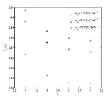
(a)

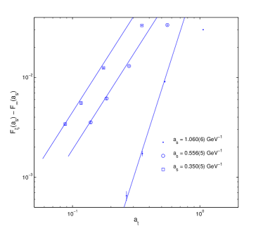
(b)

Figure 1: (a): dependence of the gauge fixing functional $F_{\xi}(a_{s})$ on the anisotropy $\xi$ at fixed spatial cut-off $a_{s}$. (b): Deviation of the gauge fixing functional from the Hamiltonian limit, $F_{\xi}(a_{s})-F_{\infty}(a_{s})$, as a function of the temporal lattice spacing $a_{t}$, together with its leading power corrections.

As the Hamiltonian limit is approached by increasing $\xi$, the functional $F$ decreases, i.e. the configurations at fixed time slice become “rougher” although $a_{s}$ is kept constant; as can be seen from the figure, the corrections with $\xi$ are several orders of magnitude higher than the Gribov noise. The leading order in the corrections to $F_{\xi}$ are well described by a power law in $\xi^{-1}\propto a_{t}$. Our best estimates for the asymptotic values $F_{\infty}$ together with the coefficient of the leading order corrections are given in Tab. 3, while the right chart of Fig. 1 shows $F_{\xi}-F_{\infty}$ versus the leading correction in $a_{t}$. For the stronger couplings, this leading correction is $\mathscr{O}(a_{t}^{4})$, while for weaker couplings we find it to scale as $\mathscr{O}(a_{t}^{2})$.

$F_{\infty}$ $c_{2}$ $c_{4}$ $a_{s}=1.060(6)$ GeV^-1 0.8333(2) $--$ 0.152(1) $a_{s}=0.556(5)$ GeV^-1 0.8620(2) 0.058(1) $--$ $a_{s}=0.350(5)$ GeV^-1 0.8737(2) 0.055(1) $--$

Table 3: Asymptotic extrapolation of $F_{\xi}$ together with the coefficient of the leading power correction of oder $\mathscr{O}(a_{t}^{4})$ ($a_{s}=1.060(6)$ GeV^-1) and $\mathscr{O}(a_{t}^{2})$ ($a_{s}=0.556(5)$ and $0.350(5)$ GeV^-1).

This sensitivity to $\xi$ (or $a_{t}$) does not only occur in the gauge fixing functional. In Ref. Burgio et al. (2008); Nakagawa et al. (2009b); Nakagawa et al. (2011) a strong dependence on the anisotropy was also seen for the temporal gluon propagator Eq. (3), although this was numerically shown to be energy (i.e. $U_{0}$) independent Burgio et al. (2009). Also, preliminary results indicate that the Gribov mass $M$ in Eq. (11) slightly increases with $\xi$, saturating to a value $M\simeq 1.2(2)$ for $\xi=3-4$. In Sec. III.3 and III.4 we will see that the ghost propagator Eq. (2) and the Coulomb potential Eq. (4), which are by definition independent of the time-like links, both turn out to be sensitive to the anisotropy.

From Fig. 1 one can infer that lattices with $\xi\gtrsim 6$ would be needed to minimize the $a_{t}$ corrections in $F$, i.e. to reach the plateau at $F_{\infty}$. Since we also need a large spatial extension $L\simeq 50$ to explore the deep infrared momentum region, the combination of these two requirements would force us to simulate on lattices of temporal extension $N_{t}\simeq 300$, beyond the computational power at our disposal. Moreover, not all observables need to be as sensitive to $\xi$ as the gauge functional. We will therefore restrict our investigation to $\xi=1\ldots 4$ and attempt to extrapolate to larger $\xi$ wherever necessary. Of course, a direct confirmation of our results on large lattices with high anisotropies would be highly desirable.

III.3 Ghost Form Factor

The ghost form factor in Coulomb gauge, Eq. (2), has been discussed in Refs. Langfeld and Moyaerts (2004); Nakagawa et al. (2007, 2009a); Burgio et al. (2010b); neither its ultraviolet nor its infrared behavior could be determined conclusively. In the UV, the primary goal is to check the sum rule for the anomalous dimensions in Eq. (7). In the IR, the main question is whether the ghost propagator is compatible with an infrared finite behaviour, as is the case in Landau gauge Bogolubsky et al. (2009). If this were true, it would of course spoil the Gribov-Zwanziger mechanism and the dual superconductor argument of Ref. Reinhardt (2008).

We calculate $d(\mathbf{p})$ by inverting the Coulomb gauge Faddeev-Popov (FP) operator through a conjugate gradient algorithm on lattices of spatial sizes up to $54^{3}$ and anisotropies up to $\xi=4$. Although for most configurations the algorithm works quite well, there are some ”exceptional” cases where very small eigenvalues of the FP operator make the inversion ill-conditioned, signaled by very bad convergence. On the other hand, we expect exactly these configurations to contribute substantially to the infrared divergence of the ghost form factor, since they lie close to the Gribov horizon. Our current procedure is to exclude such configurations from the Monte-Carlo ensemble; this obviously creates a bias in the data which potentially suppresses the ghost propagator at very low momenta.

Whether or not these near-horizon configurations have a measurable effect on the ghost propagator also depends on the frequency with which they appear within a MC sequence; contrary to Landau gauge Bogolubsky et al. (2006), this seems to be relatively stable upon improvement of the gauge fixing. In our studies we have observed an ill-defined FP operator in about one of every $300$ configurations, with very large uncertainties (i.e. there were also MC runs with over $1000$ configurations that did not show a single near-horizon configuration). Preliminary studies of individual singular configurations with improved pre-conditioners and numerics indicate that their contribution to the ghost form factor can be enhanced by up to a factor $40$ as compared to the ensemble average, again with large uncertainties due to the bad condition number. Clearly, this is a zero measure times infinite contribution problem that can only be decided by much improved statistics combined with better inversion algorithms. In this study we have not been able to resolve this issue quantitatively; the exponent which we will extract in the following must therefore be considered as a lower bound for the correct infrared behaviour.

Results for $d(\mathbf{p})$ at $\xi=1$ are shown in Fig. 2(a), while in Fig. 2(b) we give the coefficients $Z(\beta)$ needed to multiplicatively renormalize the data at different coupling, arbitrarily scaled such to let $d(\mathbf{p})\simeq 1$ at large momentum.

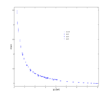
(a)

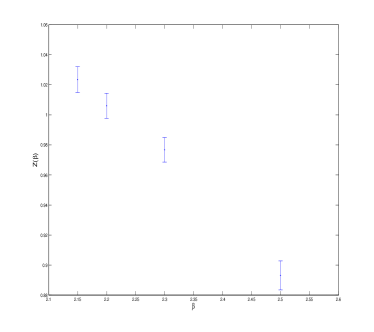
(b)

Figure 2: (a): Ghost form factor $d(|\mathbf{p}|)$ for anisotropy $\xi=1$. (b): Renormalization coefficients for the ghost propagator, as a function of the coupling $\beta$.

Although at first glance the data agree qualitatively with the above expectations, on a closer look two problems appear. First, small scaling violations can be measured within errors in the ultra-violet region; a fit to a logarithmic behavior is thus afflicted with large errors. Second, the infrared region shows two different behaviors for an intermediate momentum range $0.5$ GeV$\lesssim|\mathbf{p}|\lesssim 1.2$ GeV and a low momentum range 0.2 GeV $\lesssim|\mathbf{p}|\lesssim 0.5$ GeV. In the first regime the data are compatible with a power-law behavior

$$d(|\mathbf{p}|)\propto|\mathbf{p}|^{-\kappa},$$ (17)

with $\kappa\simeq 0.5$, while in the low-momentum region the effective $\kappa$ decreases, approaching a value $\kappa\lesssim 0.4$. By going to higher anisotropies this behavior softens and the data become more and more compatible with a stable power-law. To illustrate this effect, in Fig. 3(a) we highlight the infrared behavior showing $|\mathbf{p}|^{\kappa_{m}}d(\mathbf{p})$ for different anisotropies, where $\kappa_{m}=0.373(6)$ is the effective exponent we have measured for $L=54$, $\xi=1$ in the lowest momentum region. The data for $\xi=1$ go to a constant while for higher anisotropies a power-law still describes the data well. In Fig. 3(b) we show the IR exponents $\kappa$ obtained from three different fitting methods for each set of data at fixed anisotropy $\xi$, i.e. temporal cut-off $a_{t}$: the lower curve corresponds to a pure $|\mathbf{p}|^{-\kappa}$ behaviour cutting the data at $|\mathbf{p}|\lesssim 1.5$ GeV; the middle one adds a linear subleading correction and leaves the same cut; the higher one combines the linear correction to the power law with a cut at $|\mathbf{p}|\lesssim 1$ GeV. Fitting all these values of $\kappa$ to a constant $\kappa_{\rm gh}$, constrained to be the same for all three methods used, plus power law corrections in $a_{t}$ we find

$$\kappa_{\rm gh}=0.55(1)$$ (18)

with leading correction of order $\mathscr{O}(a_{t})$ and a $\chi^{2}$/d.o.f. $\simeq 0.3$.

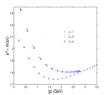
(a)

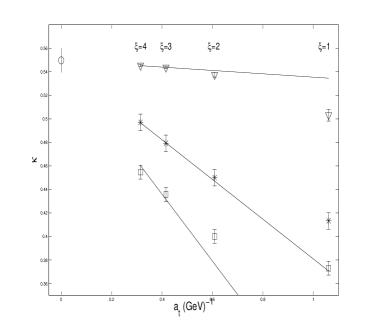
(b)

Figure 3: (a) Infrared behavior of $|\mathbf{p}|^{\kappa_{m}}\,d(\mathbf{p})$ for different anisotropies $\xi$. (b) $\kappa$ extrapolation for $a_{t}\to 0$; Different symbols correspond to different fitting methods to estimates $\kappa$; points at fixed $a_{t}$ ($\xi$) correspond to the same data set for $d(|\mathbf{p}|)$; lines give the leading correction $\propto a_{t}$ to $\kappa_{\rm gh}$.

Because of the cut on exceptional configurations discussed above we have of course introduced a bias in our data. Therefore the value in Eq. (18) can only be considered as a lower bound on the actual value of $\kappa_{\rm gh}$. Still, as far as we know, this is the first time that an IR enhanced ghost form factor can be reliably proven to exist on the lattice, making the Gribov-Zwanziger confinement scenario in Coulomb gauge fully consistent. Indeed, while in Ref. Burgio et al. (2010a) it was shown that the Gribov gluon propagator Eq. (11) is IR equivalent to the massive Landau gauge solution, in the latter case lattice simulations always give an IR finite, i.e. tree-level like ghost form factor. How this can be made to agree with the Gribov-Zwanziger mechanism is still a debated issue.

In general, although any divergence ($\kappa_{\rm gh}>0$) of the ghost form factor would be sufficient to support the Gribov-Zwanziger mechanism, the exact value of the infrared exponent $\kappa_{\rm gh}$ matters for the sum rule Eq. (7), which is violated by our findings combined with the results for Gluon propagator in Refs. Burgio et al. (2009, 2008, 2010a). There are several possible resolutions to this issue: first, our data for the ghost propagator only covers the range down to $|\mathbf{p}|\simeq 200\,\mathrm{MeV}$ with sufficient statistics and precision. Further changes in $\kappa_{\rm gh}$ at a much smaller scale $\lambda_{IR}\ll\Lambda_{QCD}$ can not be ruled out, although we currently do not see the onset of such deviations, while the appearance of an additional small scale in pure YM theory would raise a different kind of interpretation problem. Moreover, as we have explained above, our data for $\kappa_{\rm gh}$ is only a lower bound since we have neglected singular configurations from near the Gribov horizon. Whether or not these configurations contribute substantially to the ghost propagator and its exponent $\kappa_{\rm gh}$ cannot be predicted with our current computational resources. Most likely, it would also require algorithmic changes in the inversion method for ill-conditioned FP operators, and maybe even a change in the fundamental MC generator to better sample the near-horizon region in field space.

Besides these caveats at our numerical data, the origin of the sum rule Eq. (7) itself leaves room for discussion. In essence, it is based on the assumption that (i) the gluon and ghost propagators have conformal (power-like) behaviour in the infrared and (ii) the ghost-gluon vertex receives no radiative corrections (other than an overall multiplicative renormalization) at low momenta, i.e. it is essentially bare. Both results are borrowed from Landau gauge, where Taylor’s theorem gives a firm explanation why the ghost-gluon vertex is trivial as $p\to 0$. The ensuing sum rule for gluon and ghost propagator are then simple consequences, at least as long as massive solutions in the infrared can be ruled out, for which the ghost and gluon behaviour would decouple. All these assumptions are well confirmed by lattice simulations in Landau gauge.

For Coulomb gauge, however, the situation may be more involved. A careful analysis of the Slavnov-Taylor identities in Coulomb gauge exhibit a complicated interplay between transversal (spatial) and longitudinal (temporal) degrees of freedom, see Eq. (4.12) in Ref. Watson and Reinhardt (2010a). Integrating over all energies $p_{0}$ to reach the equal-time limit could therefore induce non-trivial structure in the static Green functions, even though the proof of Taylor’s theorem carries over to Coulomb gauge in the limit $|\mathbf{p}|\to 0$ at any fixed $p_{0}$. Unfortunately, no analytical calculations of the static vertex at low momenta based on the Slavnov-Taylor identities has so far been possible, and the corresponding calculation on the lattice have not been carried out. In Ref. Campagnari and Reinhardt (2012), within the Hamiltonian approach, the Dyson-Schwinger equation for the ghost-gluon vertex was solved at the one loop level and little dressing was found. Furthermore, Landau gauge calculations in three (euclidian) dimensions also exhibit little dressing of the ghost-gluon vertex; it is however unclear if these results simply carry over to the four-dimensional static quantities in Coulomb gauge.

Let us now consider the ultra-violet behavior, where exceptional configurations play no role and the situation is much clearer. As mentioned above, slight scaling violations can be measured in the data for $\xi=1$. These diminish as $\xi$ is increased and the anomalous dimension of the ghost field can be determined in the Hamiltonian limit. In Fig. 4 we compare $d(\mathbf{p})$ for the lowest and highest anisotropies $\xi$. For the latter we show our best fit to the expected asymptotic behaviour with $\gamma$ given by the sum-rule in Eq. (10); the ultra-violet mass scale from the fit is $m=0.21(1)$ GeV, cfr. Eq. (6).

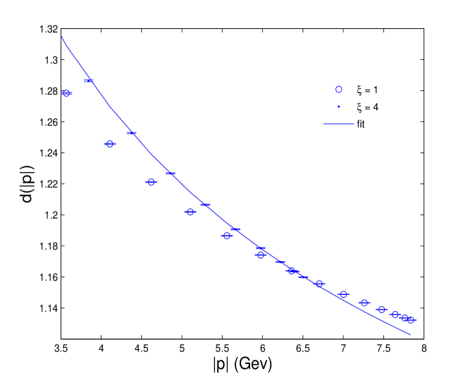
Figure 4: UV behavior of $d^{-1}(\mathbf{p})$ for different anisotropies $\xi$ compared with Eq. (6).

III.4 Coulomb Potential

The Coulomb potential, Eq. (4), has been intensively investigated in the literature Greensite and Olejnik (2003); Nakamura and Saito (2006); Nakagawa et al. (2006); Voigt et al. (2008); Nakagawa et al. (2008b, 2009b); Nakagawa et al. (2010). While there is general agreement that its infrared behavior is determined by a Coulomb string tension larger than the Wilson string tension Zwanziger (2003), the value quoted for the ratio $\sigma_{C}/\sigma$ varies among the above works.

We have calculated the Coulomb potential Eq. (4) for lattices of spatial extension up to $40^{3}$ and anisotropies up to $\xi=4$. Exceptional configurations did not play a major role in this case; this may be either due to the smaller volumes and lower statistics employed, since the computation of Eq. (4) is much more expensive than Eq. (2), or to the better pre-conditioning due to the Laplace inversion, or both. In Fig. 5 we show the infrared behavior of $|{\mathbf{p}}|^{4}\,V_{C}(\mathbf{p})/(8\pi\sigma)$ for different values of $\xi$; the reason for the normalization will be clear in the following.

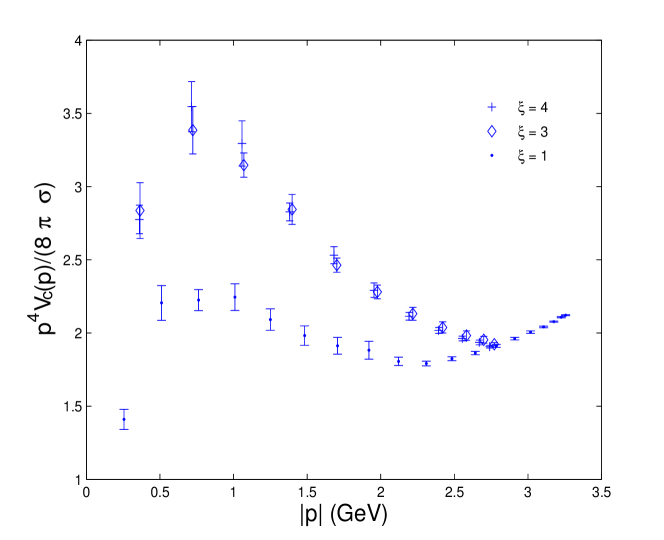
Figure 5: Infrared behavior of $|{\mathbf{p}}|^{4}\,V_{C}(\mathbf{p})/(8\pi\sigma)$ for different anisotropies $\xi$.

As in the case of the ghost form factor, we observe a change in the data in the Hamiltonian limit. The corrections due to the finite temporal resolution seem to saturate at our highest values of $\xi$, although error bars are still quite large. Also, the bending down of the data at $\simeq$ 0.5 – 1 GeV, observed in all above quoted analyses for $\xi=1$, becomes milder, although it does not disappear. Its presence should indeed not come as a surprise: at least for the physical potential $V(r)$, which we know to be given by Luscher et al. (1980)

$$V(r)=\sigma r+\mu-\frac{\pi}{12r}+\mathscr{O}(\frac{1}{r^{2}})\,,$$ (19)

we expect, after introducing a suitable IR cutoff $\lambda$ and taking $\lambda\to 0$ :

$$|{\mathbf{p}}|^{4}\,V(\mathbf{p})=8\pi\sigma+\frac{\pi^{2}}{3}|{\mathbf{p}}|^{2}+\mathscr{O}(|{\mathbf{p}}|^{3})\,,$$ (20)

since the contribution from $\mu$ in Eq. (19), which gives a term $\propto|{\mathbf{p}}|$ in Eq. (20), will vanish with $\lambda$. Thus $|{\mathbf{p}}|^{4}\,V(\mathbf{p})$ must have a minimum as $|{\mathbf{p}}|\to 0$; since its asymptotic UV behaviour is also, up to logarithmic correction, $\propto|{\mathbf{p}}|^{2}$, we only have two possibilities: either $|{\mathbf{p}}|^{4}\,V(\mathbf{p})$ is a monotonic function of $|{\mathbf{p}}|$ or, if it has some local minimum for some $|{\mathbf{p}}|_{m}>0$, then it must have a maximum in $0<|{\mathbf{p}}|_{M}<|{\mathbf{p}}|_{m}$.

If $V_{C}$ asymptotically behaves like $\sigma_{C}\,r$ the data in Fig. 5 must approach a constant as $|\mathbf{p}|\to 0$, giving direct access to the Coulomb string tension. It is natural to parametrize them as in Eq. (20):

$$\frac{|{\mathbf{p}}|^{4}\,V_{C}(\mathbf{p})}{8\pi\sigma}=\frac{\sigma_{C}}{\sigma}+\alpha|{\mathbf{p}}|+\gamma|{\mathbf{p}}|^{2}+\mathscr{O}(|{\mathbf{p}}|^{3})\,.$$ (21)

where we would expect $\gamma>0$ and $\alpha\to 0$ in the thermodynamic limit. Fitting the data to Eq. (21) and introducing different cuts at different momenta we obtain for the Coulomb string tension

$$\sigma_{C}=2.2(2)\,\sigma\,.$$ (22)

Notice that, even though we don’t have much data in the IR region, if we optimistically constrain $\alpha\equiv 0$ we obtain a higher value for the Coulomb string tension, $\sigma_{C}=2.5(1)\,\sigma$. Better statistics and data from larger lattices and/or anisotropies in the low momentum region would of course be welcome to improve the result.

IV Conclusions

We have shown that a sufficient approach to the Hamiltonian limit, which on the lattice translates into anisotropic lattices with a high temporal resolution, is crucial for a successful investigation of the ghost form factor and the Coulomb potential. The effect of the anisotropy on static correlators lies in the different dynamics for fixed spatial lattice spacing $a_{s}$ as $a_{t}$ decreases, as we have shown in Sec. III.2. This explains the dependence on $\xi$ found also for explicitly energy independent observables that can be evaluated in a single time slice.

In Sec. III.3 we have shown that the infrared exponent of the ghost form factor saturates at $\kappa_{\rm gh}\approx 0.55(1)$ when taking the Hamiltonian limit. Although our estimate may only be a lower bound due to the contribution of near-horizon configurations, the infrared divergence of the ghost form factor confirms the Gribov-Zwanziger Gribov (1978); Zwanziger (1997) confinement mechanism and the vanishing of the dielectric function for the Yang-Mills vacuum Reinhardt (2008). We have also confirmed quantitatively the sum rule for the anomalous dimensions of the static gluon and ghost fields in Coulomb gauge. The similar sum rule prediction in the infrared would require $\kappa_{\rm gh}=1$ in order to be compatible with the Gribov formula confirmed in ref. Burgio et al. (2010a). This is clearly violated by our best fit $\kappa_{\rm gh}\approx 0.55(1)$. We have discussed possible arguments to resolve this discrepancy, by critically analyzing both our data and the origin of the sum rule itself. A conclusive settlement of this issue must be left to a future investigation. Finally, in Sec. III.4 we have shown that the Coulomb potential is linearly rising in position space, and the corresponding Coulomb string tension settles nicely in the Hamiltonian limit $\xi\to\infty$, where we extract a value of $\sigma_{C}\simeq 2.2\,\sigma$.

As indicated above, future investigations in this direction should concentrate on the ghost form factor and Coulomb potential on much larger spatial lattices to probe lower momenta, with improved statistics and better numerics to tackle the rare near-horizon configurations. This may help to settle the remaining question of the infrared sum rule for the exponents in the power-law of the low order Green functions.

References

- Gribov (1978) V. N. Gribov, Nucl. Phys. B139, 1 (1978).
- Zwanziger (1997) D. Zwanziger, Nucl. Phys. B485, 185 (1997), eprint hep-th/9603203.
- Faddeev and Popov (1967) L. D. Faddeev and V. N. Popov, Phys. Lett. B25, 29 (1967).
- Singer (1978) I. M. Singer, Commun. Math. Phys. 60, 7 (1978).
- Killingback (1984) T. P. Killingback, Phys. Lett. B138, 87 (1984).
- Becchi et al. (1976) C. Becchi, A. Rouet, and R. Stora, Annals Phys. 98, 287 (1976).
- Tyutin (1975) I. V. Tyutin (1975), eprint 0812.0580.
- Burgio et al. (1998) G. Burgio, F. Di Renzo, G. Marchesini, and E. Onofri, Phys. Lett. B422, 219 (1998), eprint hep-ph/9706209.
- Akhoury and Zakharov (1998) R. Akhoury and V. I. Zakharov, Phys. Lett. B438, 165 (1998), eprint hep-ph/9710487.
- Boucaud et al. (2000) P. Boucaud et al., JHEP 04, 006 (2000), eprint hep-ph/0003020.
- Dudal et al. (2010) D. Dudal, O. Oliveira, and N. Vandersickel (2010), eprint 1002.2374.
- Vandersickel and Zwanziger (2012) N. Vandersickel and D. Zwanziger (2012), eprint 1202.1491.
- Dudal and Sorella (2012) D. Dudal and S. P. Sorella (2012), eprint 1205.3934.
- Christ and Lee (1980) N. H. Christ and T. D. Lee, Phys. Rev. D22, 939 (1980).
- Szczepaniak and Swanson (2002) A. P. Szczepaniak and E. S. Swanson, Phys. Rev. D65, 025012 (2002), eprint hep-ph/0107078.
- Feuchter and Reinhardt (2004a) C. Feuchter and H. Reinhardt (2004a), eprint hep-th/0402106.
- Feuchter and Reinhardt (2004b) C. Feuchter and H. Reinhardt, Phys. Rev. D70, 105021 (2004b), eprint hep-th/0408236.
- Reinhardt and Watson (2009) H. Reinhardt and P. Watson, Phys. Rev. D79, 045013 (2009), eprint 0808.2436.
- Reinhardt and Schleifenbaum (2009) H. Reinhardt and W. Schleifenbaum, Annals Phys. 324, 735 (2009), eprint 0809.1764.
- Kugo and Ojima (1979) T. Kugo and I. Ojima, Prog. Theor. Phys. Suppl. 66, 1 (1979).
- Burgio et al. (2000) G. Burgio, R. De Pietri, H. A. Morales-Tecotl, L. F. Urrutia, and J. D. Vergara, Nucl. Phys. B566, 547 (2000), eprint hep-lat/9906036.
- Reinhardt (2008) H. Reinhardt, Phys. Rev. Lett. 101, 061602 (2008), eprint 0803.0504.
- Zwanziger (2003) D. Zwanziger, Phys. Rev. Lett. 90, 102001 (2003), eprint hep-lat/0209105.
- Drell et al. (1979) S. D. Drell, H. R. Quinn, B. Svetitsky, and M. Weinstein, Phys. Rev. D19, 619 (1979).
- Greensite (1979) J. P. Greensite, Nucl. Phys. B158, 469 (1979).
- Arisue et al. (1983) H. Arisue, M. Kato, and T. Fujiwara, Prog. Theor. Phys. 70, 229 (1983).
- Velikson and Weingarten (1985) B. Velikson and D. Weingarten, Nucl. Phys. B249, 433 (1985).
- Hecht et al. (1993) M. W. Hecht et al., Phys. Rev. D47, 285 (1993), eprint hep-lat/9208005.
- Kogan and Kovner (1995) I. I. Kogan and A. Kovner, Phys. Rev. D52, 3719 (1995), eprint hep-th/9408081.
- Karabali and Nair (1996) D. Karabali and V. P. Nair, Nucl. Phys. B464, 135 (1996), eprint hep-th/9510157.
- Brown (1998) W. E. Brown, Int. J. Mod. Phys. A13, 5219 (1998), eprint hep-th/9711189.
- Brown and Kogan (1999) W. E. Brown and I. I. Kogan, Int. J. Mod. Phys. A14, 799 (1999), eprint hep-th/9705136.
- Karabali et al. (1998) D. Karabali, C.-j. Kim, and V. P. Nair, Phys. Lett. B434, 103 (1998), eprint hep-th/9804132.
- Leigh et al. (2006) R. G. Leigh, D. Minic, and A. Yelnikov, Phys. Rev. Lett. 96, 222001 (2006), eprint hep-th/0512111.
- Greensite and Olejnik (2008) J. Greensite and S. Olejnik, Phys. Rev. D77, 065003 (2008), eprint 0707.2860.
- Quandt et al. (2010) M. Quandt, H. Reinhardt, and G. Burgio, Phys. Rev. D81, 065016 (2010), eprint 1001.3699.
- Reinhardt et al. (2012) H. Reinhardt, M. Quandt, and G. Burgio, Phys.Rev. D85, 025001 (2012), eprint 1110.2927.
- Langfeld and Moyaerts (2004) K. Langfeld and L. Moyaerts, Phys. Rev. D70, 074507 (2004), eprint hep-lat/0406024.
- Voigt et al. (2007) A. Voigt, E.-M. Ilgenfritz, M. Muller-Preussker, and A. Sternbeck, PoS LAT2007, 338 (2007), eprint 0709.4585.
- Nakagawa et al. (2008a) Y. Nakagawa, A. Nakamura, T. Saito, and H. Toki, Mod. Phys. Lett. A23, 2352 (2008a).
- Nakagawa et al. (2009a) Y. Nakagawa et al., Phys. Rev. D79, 114504 (2009a), eprint 0902.4321.
- Burgio et al. (2009) G. Burgio, M. Quandt, and H. Reinhardt, Phys. Rev. Lett. 102, 032002 (2009), eprint 0807.3291.
- Burgio et al. (2008) G. Burgio, M. Quandt, and H. Reinhardt, PoS CONFINEMENT8, 051 (2008), eprint 0812.3786.
- Burgio et al. (2010a) G. Burgio, M. Quandt, and H. Reinhardt, Phys. Rev. D81, 074502 (2010a), eprint 0911.5101.
- Burgio et al. (2012) G. Burgio, M. Schrock, H. Reinhardt, and M. Quandt (2012), eprint 1204.0716.
- Jackiw et al. (1978) R. Jackiw, I. Muzinich, and C. Rebbi, Phys. Rev. D17, 1576 (1978).
- Zwanziger (1998) D. Zwanziger, Nucl.Phys. B518, 237 (1998).
- Epple et al. (2007) D. Epple, H. Reinhardt, and W. Schleifenbaum, Phys. Rev. D75, 045011 (2007), eprint hep-th/0612241.
- Epple et al. (2008) D. Epple, H. Reinhardt, W. Schleifenbaum, and A. P. Szczepaniak, Phys. Rev. D77, 085007 (2008), eprint 0712.3694.
- Schleifenbaum et al. (2006) W. Schleifenbaum, M. Leder, and H. Reinhardt, Phys. Rev. D73, 125019 (2006), eprint hep-th/0605115.
- Leder et al. (2011) M. Leder, J. M. Pawlowski, H. Reinhardt, and A. Weber, Phys.Rev. D83, 025010 (2011), eprint 1006.5710.
- Watson and Reinhardt (2007) P. Watson and H. Reinhardt, Phys. Rev. D76, 125016 (2007), eprint 0709.0140.
- Watson and Reinhardt (2008) P. Watson and H. Reinhardt, Phys. Rev. D77, 025030 (2008), eprint 0709.3963.
- Watson and Reinhardt (2010a) P. Watson and H. Reinhardt, Eur.Phys.J. C65, 567 (2010a), eprint 0812.1989.
- Watson and Reinhardt (2010b) P. Watson and H. Reinhardt (2010b), eprint 1007.2583.
- Andrasi and Taylor (2011) A. Andrasi and J. C. Taylor, Annals Phys. 326, 1053 (2011), eprint 1010.5911.
- Andrasi and Taylor (2012) A. Andrasi and J. Taylor (2012), eprint 1204.1722.
- Campagnari et al. (2009a) D. R. Campagnari, H. Reinhardt, and A. Weber, Phys. Rev. D80, 025005 (2009a), eprint 0904.3490.
- Campagnari et al. (2009b) D. Campagnari, A. Weber, H. Reinhardt, F. Astorga, and W. Schleifenbaum (2009b), eprint 0910.4548.
- Cucchieri and Zwanziger (2002) A. Cucchieri and D. Zwanziger, Phys. Rev. D65, 014001 (2002), eprint hep-lat/0008026.
- Burgio et al. (2003) G. Burgio, A. Feo, M. J. Peardon, and S. M. Ryan (TrinLat), Phys. Rev. D67, 114502 (2003), eprint hep-lat/0303005.
- Nakagawa et al. (2009b) Y. Nakagawa, A. Nakamura, T. Saito, and H. Toki, PoS LAT2009, 230 (2009b), eprint 0911.2550.
- Nakagawa et al. (2011) Y. Nakagawa, A. Nakamura, T. Saito, and H. Toki, Phys.Rev. D83, 114503 (2011), eprint 1105.6185.
- Kogut and Susskind (1975) J. B. Kogut and L. Susskind, Phys. Rev. D11, 395 (1975).
- Kogut et al. (1979) J. B. Kogut, R. B. Pearson, and J. Shigemitsu, Phys. Rev. Lett. 43, 484 (1979).
- Svetitsky and Yaffe (1982) B. Svetitsky and L. G. Yaffe, Nucl. Phys. B210, 423 (1982).
- Burgio et al. (2004) G. Burgio, A. Feo, M. J. Peardon, and S. M. Ryan, Nucl. Phys. Proc. Suppl. 129, 396 (2004), eprint hep-lat/0310036.
- Morningstar and Peardon (1999) C. J. Morningstar and M. J. Peardon, Phys. Rev. D60, 034509 (1999), eprint hep-lat/9901004.
- Klassen (1998) T. R. Klassen, Nucl. Phys. B533, 557 (1998), eprint hep-lat/9803010.
- Ishiguro et al. (2002) K. Ishiguro, T. Suzuki, and T. Yazawa, JHEP 01, 038 (2002), eprint hep-lat/0112022.
- Bloch et al. (2004) J. C. R. Bloch, A. Cucchieri, K. Langfeld, and T. Mendes, Nucl. Phys. B687, 76 (2004), eprint hep-lat/0312036.
- Bogolubsky et al. (2006) I. L. Bogolubsky et al., Phys. Rev. D74, 034503 (2006), eprint hep-lat/0511056.
- Bogolubsky et al. (2008) I. L. Bogolubsky et al., Phys. Rev. D77, 014504 (2008), eprint 0707.3611.
- Not (a) Notice that the complexity of our gauge fixing algorithm scales with the spatial volume since all time slices are fixed independently.
- Nakagawa et al. (2007) Y. Nakagawa, A. Nakamura, T. Saito, and H. Toki, Phys. Rev. D75, 014508 (2007), eprint hep-lat/0702002.
- Burgio et al. (2010b) G. Burgio, M. Quandt, M. Schrock, and H. Reinhardt, PoS LATTICE2010, 272 (2010b), eprint 1011.0560.
- Bogolubsky et al. (2009) I. L. Bogolubsky, E. M. Ilgenfritz, M. Muller-Preussker, and A. Sternbeck, Phys. Lett. B676, 69 (2009), eprint 0901.0736.
- Campagnari and Reinhardt (2012) D. R. Campagnari and H. Reinhardt, Phys.Lett. B707, 216 (2012), eprint 1111.5476.
- Greensite and Olejnik (2003) J. Greensite and S. Olejnik, Phys. Rev. D67, 094503 (2003), eprint hep-lat/0302018.
- Nakamura and Saito (2006) A. Nakamura and T. Saito, Prog. Theor. Phys. 115, 189 (2006), eprint hep-lat/0512042.
- Nakagawa et al. (2006) Y. Nakagawa, T. Saito, H. Toki, and A. Nakamura, PoS LAT2006, 071 (2006), eprint hep-lat/0610128.
- Voigt et al. (2008) A. Voigt, E. M. Ilgenfritz, M. Muller-Preussker, and A. Sternbeck, Phys. Rev. D78, 014501 (2008), eprint 0803.2307.
- Nakagawa et al. (2008b) Y. Nakagawa, A. Nakamura, T. Saito, and T. Toki, Mod. Phys. Lett. A23, 2348 (2008b).
- Nakagawa et al. (2010) Y. Nakagawa, A. Nakamura, T. Saito, and H. Toki, Phys. Rev. D81, 054509 (2010), eprint 1003.4792.
- Luscher et al. (1980) M. Luscher, K. Symanzik, and P. Weisz, Nucl.Phys. B173, 365 (1980).
- Not (b) A Yukawa fall-off is convenient to perform the Fourier integrals, but any other IR cutoff, e.g. a finite lattice size, will work as well. Of course, the two limits and do not commute; the thermodinamic limit must be taken first.