Reconstruction of Planar Domains

from Partial Integral Measurements

D. Batenkov¹, V. Golubyatnikov ^2,3, Y. Yomdin ¹

1. Weizmann Institute of Science, Rehovot, Israel.

2. Sobolev Institute of Mathematics, Novosibirsk, Russia.

3. Novosibirsk State University, Russia.

Abstract

We consider the problem of reconstruction of planar domains from their moments. Specifically, we consider domains with boundary which can be represented by a union of a finite number of pieces whose graphs are solutions of a linear differential equation with polynomial coefficients. This includes domains with piecewise-algebraic and, in particular, piecewise-polynomial boundaries. Our approach is based on one-dimensional reconstruction method of [5] and a kind of “separation of variables” which reduces the planar problem to two one-dimensional problems, one of them parametric. Several explicit examples of reconstruction are given.

Another main topic of the paper concerns “invisible sets” for various types of incomplete moment measurements. We suggest a certain point of view which stresses remarkable similarity between several apparently unrelated problems. In particular, we discuss zero quadrature domains (invisible for harmonic polynomials), invisibility for powers of a given polynomial, and invisibility for complex moments (Wermer’s theorem and further developments). The common property we would like to stress is a “rigidity” and symmetry of the invisible objects.

————————————————

This research was supported by the ISF, Grants No. 639/09, and by the Minerva Foundation.

1 Introduction

In this paper we continue our study of nonlinear problems of reconstruction of multidimensional objects from incomplete collection of integral measurements. The paper has two parts, closely related but different in their goals. In the first part we present a method of reconstruction of planar domains of a certain special class from finite collections of moments. In the second part we discuss the structure of sets and functions “invisible” for a certain collection of moment measurements.

In more detail, the object we would like to reconstruct is a 2-dimensional finite domain $G\subset{\mathbb{R}}^{2}$ which we assume to belong to a certain finite-dimensional family $G_{\lambda}$ specified by a finite number of discrete and continuous parameters $\lambda$. Specifically, we shall assume that the boundary of $G$ is a union of a finite number of pieces whose graphs are solutions of a linear differential equation with polynomial coefficients.

The measurements are represented by finite collections of the moments $m_{\alpha,\beta}$ of the characteristic function $\chi_{G}(x,y)$ of the domain $G$:

$$m_{\alpha,\beta}=\iint_{R^{2}}\,\chi_{G}(x,y)\cdot x^{\alpha}y^{\beta}dxdy.$$ (1.1)

Our main problem is to provide an explicit (and potentially efficient) reconstruction method, and, in particular, to estimate a minimal possible set of these moments sufficient for unique reconstruction of the domain $G$.

Similar inverse problems have been intensively studied, including reconstruction from their moments of polygons, of quadrature domains, of certain “dynamic” semi-algebraic sets, see [7, 8, 17, 20, 33] and references therein. In a more general context the problem of domain reconstruction from its moments appears as a part of broad field of inverse problems in Potential Theory (see, for example, [36]). Rather similar questions arise in reconstruction from tomography measurements ([18, 19, 31]).

Our approach is based on one-dimensional reconstruction method of [5] applicable to piecewise continuous functions satisfying on each continuity interval a linear differential equation with polynomial coefficients. Then we use a kind of “separation of variables” which reduces the planar problem to two one-dimensional problems, one of them parametric.

We expect that a reconstruction method for piecewise-smooth functions given in [9] can be extended in a similar way also to planar and higher dimensional piecewise-smooth functions.

The second part of the present paper is devoted to “invisible sets” for various types of incomplete measurements. Here we do not provide new results (besides a couple of examples), but rather suggest a certain point of view which stresses remarkable similarity between several apparently unrelated “moment vanishing” problems. In particular, we discuss zero quadrature domains (invisible for harmonic polynomials), invisibility for polynomials annihilating other partial differential operators, invisibility for powers of a given polynomial, and invisibility for complex moments (Wermer’s theorem and further developments). In all these cases we stress a common property of “rigidity” and symmetry of the invisible objects.

2 One-dimensional case

Reconstruction problem in dimension one has been settled in a pretty satisfactory way for many important finite-dimensional families of functions. This includes linear combinations of shifts of known functions, signals with “finite rate of innovation”, piecewise D-finite functions which we use below, piecewise-smooth functions, and many other cases (see [5, 6, 9, 14, 35] and references therein).

2.1 Piecewise D-finite reconstruction

Let $g(x)$ be a function with a support $[a,b]\subset{\mathbb{R}}^{1}$, satisfying the following condition: there exists a finite set of ${\cal K}+2$ points $a=\xi_{0}<\xi_{1}<\ldots<\xi_{{\cal K}+1}=b$, such that on each segment $[\xi_{n},\xi_{n+1}],\ n=0,1,\ldots{\cal K}$, the function $g(x)$ is continuous and satisfies there a linear differential equation

$$D_{n}g(x)=\sum\limits_{j=0}^{N}p_{n,j}(x)\left(\frac{d^{j}g}{dx^{j}}\right)=0$$ (2.1)

with polynomial coefficients $p_{n,j}(x)=\sum\limits_{i=0}^{k_{n,j}}a_{n,i,j}x^{i}$, $\,p_{N,j}\neq 0$ on $[a,b]$. At the points $\xi_{n}$ the function $\,g(x)\,$ may have jumps. Such functions are described by a finite collection of discrete and continuous parameters, and they are called piecewise $D$-finite. Without loss of generality (at least theoretically) we can assume that all the operators $D_{n}=D$ are the same. In particular, piecewise-algebraic, and, specifically, piecewise-polynomial functions belong to this class. In the last case the differential operator is $D=\frac{d^{N+1}}{dx^{N+1}}$, where $N$ is the maximal degree of the polynomial pieces of $g$.

It was shown in [5] that the collection of “discrete” parameters ${\cal K}$, $N$, $\{k_{n,j}\}$, together with a sufficiently large collection of the moments

$$m_{\alpha}=\int\nolimits_{a}^{b}g(x)\cdot x^{\alpha}dx,\quad\alpha=0,1,2,\ldots,\mu$$

determine uniquely any $D$-finite function $g(x)$ with all the points $\xi_{0},\ldots\xi_{{\cal K}+1}$ of its possible discontinuity, as well as the coefficients of the differential operator $D$.

For piecewise-polynomial functions the number $\mu$ of the moments required for reconstruction, depends only on the discrete data: the number of jumps ${\cal K}$ and on the maximal degree $N$ of the pieces. It is shown in [5] that in piecewise-polynomial case

$$\mu=\mu({\cal K},N)={\rm max\,}\biggl{\{}2(N+1)\mathcal{K}-2,(\mathcal{K}+1)(N+1)\biggr{\}}.$$

A similar, but more complicated expression for $\mu$ can be written in piecewise-algebraic case. However, for general $D$-finite functions, with respect to a general second (and higher) order differential operators $D$, the number $\mu$ may depend also on specific coefficients of $D$.

Let us give a very simple example of this latter phenomenon. Let $L_{n}(x)$ be the $n$-th Legendre polynomial, defined as $L_{n}(x)={1\over{2^{n}n!}}{{d^{n}}\over{dx^{n}}}[(x^{2}-1)^{n}].$ Legendre polynomials are pairwise orthogonal on $[-1,1]$ and they satisfy the second order Legendre differential equation ${d\over{dx}}[(1-x^{2}){d\over{dx}}L_{n}(x)]+n(n+1)L_{n}(x)=0.$ Since $L_{j}(x),\ j\leq n,$ form a basis of the space of all polynomials of degree $n$ we conclude that $L_{n}(x)$ is orthogonal to $1,x,x^{2},\dots,x^{n-1}$. Hence the moments $m_{j}(L_{n})=\int_{-1}^{1}x^{j}L_{n}(x)dx$ vanish for $j=0,1,\dots,n-1$. We conclude that a $D$-finite function $L_{n}(x)$ on $[-1,1]$ cannot be reconstructed from less than $n+1$ its moments. So $\mu$ above depends not only on the order and degree of the Legendre operator, but also on a specific value of the parameter $n$ in it.

Notice that the leading coefficient of the Legendre equation vanishes at both the endpoints $-1,1$ of the interval.

The reconstruction procedure described in [5] consists of solving certain linear and non-linear algebraic equations whose coefficients are expressed through the moments $m_{\alpha}$. These equations have a very specific structure which we illustrate in the next section with the simplest example of the classical “Prony system”. The last step requires also finding a basis of the solution space of the differential equation $Dg=0$.

We shall apply below this reconstruction procedure, referring to it as to Procedure 1.

2.2 Prony system

Prony system appears as we try to solve a very simple version of the shifts reconstruction problem. Consider $F(x)=\sum_{j=1}^{N}a_{j}\delta(x-x_{i})$. We use as measurements the polynomial moments

$$m_{n}=\int_{-\infty}^{\infty}F(x)x^{n}dx.$$

After substituting $F$ into this integral we get $m_{n}=\int\sum_{j=1}^{N}a_{i}\delta(x-x_{j})x^{n}dx=\sum_{j=1}^{N}a_{j}x_{j}^{n}.$ Considering $a_{i}$ and $x_{i}$ as unknowns, we obtain equations

$$m_{n}=\sum_{j=1}^{N}a_{j}x_{j}^{n},\ n=0,1\dots.$$ (2.2)

This infinite set of equations is called Prony system. It can be traced at least to R. de Prony (1795, [32]) and it is used in a wide variety of theoretical and applied fields. See, for example, [6, 35] and references therein for a very partial list, as well as for a sketch of one of the solution methods. This method requires $2N$ equations from (2.2). It allows first to find the number of nonzero coefficients $a_{j}$. Then $a_{j}$ and $x_{j}$ are found via solving first a Hankel-type linear system of equations with coefficients formed by the moments $m_{l}$, interpreting the solution as the coefficients of a certain polynomial, and finding all the roots of this polynomial.

We shall apply below this Prony solution procedure in our specific situation, referring to it as to Procedure 2.

3 Main result

We assume that the domain $G\subset{\mathbb{R}}^{2}$ to be reconstructed has a “D-finite boundary”. More accurately, we have the following definition:

Definition 3.1

A compact domain $G\subset{\mathbb{R}}^{2}$ is called $D$-finite if the boundary $\partial G$ is a union of $\kappa$ segments $S_{j}$ with the following property: there exists a linear differential operator $D$ of the form (2.1) and with the leading coefficient not vanishing for $x$ in the projection of $G$, such that each $S_{j}$ is the graph of a function $y=\psi_{j}(x)$ satisfying $D\psi_{j}=0$.

In particular, if each $S_{j}$ is a graph of an algebraic function $y=\psi_{j}(x)$ and all the branches of these algebraic functions are regular over the projection of $G$, then $G$ is $D$-finite. The simplest but still important example of $D$-finite domain is when all $\psi_{j}$ are polynomials.

We do not restrict the topological type of $G$ — it may have “holes”.

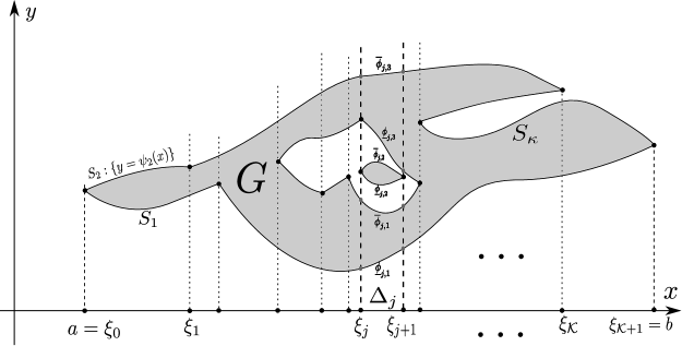
Figure 1: Schematic representation of the domain $G$.

Before we formulate the main result, let us introduce some notations. Let $[a,b]$ be the projection of $G$ onto the $x$-axis, and let $a=\xi_{0}<\xi_{1}<\ldots<\xi_{{\cal K}+1}=b$ be all the projections of the endpoints of the segments $S_{j}$ of the boundary $\partial G$ (see Figure 1). Certainly, ${\cal K}\leq\kappa$, while the maximal number of the intersection points of $\partial G$ with vertical lines is at most $\kappa-1$.

Write the linear differential operator $D$ in Definition 3.1 as

$$Dg(x)=\sum\limits_{j=0}^{N}p_{j}(x)\frac{d^{j}g}{dx^{j}}(x),$$ (3.1)

where $p_{j}(x)=\sum\limits_{i=0}^{k_{j}}a_{i,j}x^{i}$.

Theorem 3.1

Any $D$-finite domain with the discrete parameters $\kappa,N,k_{j}$ can be uniquely reconstructed from a collection of double moments

$$m_{\alpha,\beta}=\iint_{R^{2}}\,\chi_{G}(x,y)\cdot x^{\alpha}y^{\beta}dxdy,\ 0\leq\alpha\leq M(\kappa,N,k_{j}),\ 0\leq\beta\leq 2(\kappa-1).$$ (3.2)

The reconstruction procedure requires solving of certain linear and non-linear algebraic equations whose coefficients are expressed through the moments $m_{\alpha,\beta}$, and solving equation $Du=0$ with specific numerical coefficients found in previous stages.

Proof: Denote by $\Delta_{j}$ the interval $[\xi_{j},\xi_{j+1}],\ j=0,\dots,{\cal K}.$ Over each $\Delta_{j}$ the domain $G$ is a union of $s_{j}\leq{1\over 2}(\kappa-1)$ strips $\underline{\phi}_{j,l}\leq y\leq\overline{\phi}_{j,l},\ ,l=1,\dots,s_{j}$, (see Figure 1). We have

$$m_{\alpha,\beta}=\int_{a}^{b}x^{\alpha}\Psi_{\beta}(x)dx=\sum_{j=0}^{{\cal K}}\int_{\Delta_{j}}x^{\alpha}\Psi_{\beta,j}(x)dx,$$ (3.3)

where for $x\in\Delta_{j}$

$$\Psi_{\beta,j}(x)=\int_{\underline{\phi}_{j,1}(x)}^{\overline{\phi}_{j,s_{j}}(x)}y^{\beta}\chi_{G}(x,y)dy={1\over{\beta+1}}\sum_{l=1}^{s_{j}}[\overline{\phi}^{\beta+1}_{j,l}(x)-\underline{\phi}^{\beta+1}_{j,l}(x)].$$ (3.4)

The first conclusion is that for each $\beta\geq 0$ the function $\Psi_{\beta}$ is piecewise $D$-finite. Indeed, on each interval $\Delta_{j},\ j=0,\dots,{\cal K},\ \Psi_{\beta}=\Psi_{\beta,j}$ is a linear combination of the $\beta$-th powers of the functions $\underline{\phi}_{j,l},\overline{\phi}_{j,l},\ l=1,\dots,s_{j}$ which, by the assumption on $G$, satisfy $D\psi=0$. Hence $\Psi_{\beta}$ (i.e. each $\Psi_{\beta,j}$) satisfies another linear differential equation with polynomial coefficients $D_{\beta}\Psi_{\beta}=0$. The operator $D_{\beta}$ depends only on $D$, in particular, its order and degree depend only on the order and degree of $D$, and it has no singularities on $[a,b]$, if $D$ possesses this property.

We can find one-dimensional moments of $\Psi_{\beta}$ via (3.3):

$$m_{\alpha}(\Psi_{\beta})=\int_{a}^{b}x^{\alpha}\Psi_{\beta}(x)dx=m_{\alpha,\beta}.$$ (3.5)

Now we apply one-dimensional Procedure 1 from Section 2.1, and reconstruct $\Psi_{\beta}$ from the moments $m_{\alpha,\beta},\ \alpha=0,1,\dots,\mu_{\beta}\leq M(\kappa,N,k_{j})$ for each $\beta=0,1,\dots,2(\kappa-1)$. The reconstruction procedure requires solving of certain linear and non-linear algebraic equations whose coefficients are expressed through the moments $m_{\alpha,\beta}$, and solving differential equations $D_{\beta}u=0$ with specific numerical coefficients found in previous stages. Ultimately, $\Psi_{\beta}(x)=\Psi_{\beta,j}(x)$ is represented on each interval $\Delta_{j}$ as a linear combination of the basis solutions of $D_{\beta}u=0$.

Next, for each fixed $x\in\Delta_{j}$ we consider equalities (3.4) for different $\beta$ as a system of equations for the unknowns $\underline{\phi}_{j,l}(x),\overline{\phi}_{j,l}(x)$, with the known by now right hand side $\Psi_{\beta,j}(x)$. This system of equations is a special case of the Prony system, as described in the previous section. Here the amplitudes $a_{j}$ are known to be $\pm 1$. (3.4) does not give the first equation in the Prony system, but it is just the sum of the amplitudes $a_{j}$, and we know it to be zero. So finally, we apply Procedure 2 and solve system (3.4), reconstructing the functions $\underline{\phi}_{j,l}(x),\overline{\phi}_{j,l}(x)$ for each $x\in\Delta_{j}$. Now the functions $\underline{\phi}_{j,l}(x),\overline{\phi}_{j,l}(x)$ for $j=0,\dots,{\cal K},\ l=1,\dots,s_{j},$ completely determine the domain $G$. Theorem 3.1 is proved.

As it was mentioned above, for the case of algebraic boundary segments explicit bounds can be given on the number of the moments required for reconstruction. We provide these bounds in the case of polynomial boundaries, where the expressions are relatively simple and pretty sharp.

Theorem 3.2

Under the assumptions of Theorem 3.1 let us assume additionally that each boundary segment $S_{j}$ is a graph of a polynomial $y=\psi_{j}(x)$ of degree at most $d$. Then the domain $G$ can be uniquely reconstructed from a collection of double moments

$$\{m_{\alpha,\beta}:\;0\leq\beta\leq 2(\kappa-1),\;0\leq\alpha\leq M(N,\kappa,\beta)\}$$

where

$$M(d,\kappa,\beta)={\rm max\,}\biggl{\{}2(\beta N+1)\kappa-2,(\kappa+1)(\beta N+1)\biggr{\}}.$$

Proof: The functions $\Psi_{\beta}$ constructed in the proof of Theorem 3.1 are now piecewise-polynomials of degree at most $\beta N$, and the conclusion follows from the corresponding result of [5] given in Section 2 above.

4 Examples of Explicit Reconstruction

The main object considered in this section is a compact plane domain bounded by a part of an elliptic curve

$$y^{2}=ax^{3}+bx^{2}+cx+d\equiv f(x).$$

We assume that the roots $x_{1}<x_{2}$, and $\,x_{3}$ of the equation $f(x)=0$ are real, and that the function $f(x)$ is positive on the interval $(x_{1},x_{2})$. Hence, the equation $y^{2}=ax^{3}+bx^{2}+cx+d\,$ defines a compact domain $G\subset{\mathbb{R}}^{2}$.

Consider a finite collection of corresponding moments

$$m_{\alpha,\beta}=\int_{G}x^{\alpha}\cdot y^{\beta}\,dx\,dy.$$

Since the domain $G$ is symmetric with respect to the axis $Ox$, we have $m_{\alpha,\beta}=0$ for odd values of $\beta$, and

$$m_{\alpha,2\beta}=\frac{2}{2\beta+1}\int_{x_{1}}^{x_{2}}x^{\alpha}\cdot(ax^{3}+bx^{2}+cx+d)^{\beta+1/2}dx.$$

In order to simplify the formulae below, we introduce one more notation:

$$M_{\alpha,2\beta}=\frac{2\beta+1}{2}\cdot m_{\alpha,2\beta},$$

and we call it ”Moment”. So, the equation (4.2) implies that

$$M_{\alpha,2\beta+2}=a\cdot M_{\alpha+3,2\beta}+b\cdot M_{\alpha+2,2\beta}+c\cdot M_{\alpha+1,2\beta}+d\cdot M_{\alpha,2\beta}.$$

Our task is to determine the curve (4.1) from a finite (possibly minimal) collection of the Moments $M_{\alpha,2\beta}$.

Let us calculate the Moments $M_{\alpha,2\beta}$ for small values of the indices:

$M_{0,2}=a\cdot M_{3,0}+b\cdot M_{2,0}+c\cdot M_{1,0}+d\cdot M_{0,0}$; (4.4)

$M_{1,2}=a\cdot M_{4,0}+b\cdot M_{3,0}+c\cdot M_{2,0}+d\cdot M_{1,0}$.

Hence, one can obtain a system of relations with unknown coefficients $a,b,c,d$, and to verify compatibility of the ”data” $\{M_{\alpha,\beta}\}$.

Here are two more methods of construction of similar relations:

a). Consider the Moment

$$M_{\alpha,2}=\int_{x_{1}}^{x_{2}}x^{\alpha}\cdot(ax^{3}+bx^{2}+cx+d)^{3/2}dx.$$

Since $f(x_{1})=f(x_{2})=0$, integrating by parts:

$du=x^{\alpha}dx$, $\,\,v=(ax^{3}+bx^{2}+cx+d)^{3/2}$, shows that:

$$M_{\alpha,2}=-\frac{3}{2(\alpha+1)}\cdot(3a\cdot M_{\alpha+3,0}+2b\cdot M_{\alpha+2,0}+c\cdot M_{\alpha+1,0}).$$

In the cases $\alpha=1$, and $\alpha=0$ we get

$$-\frac{4}{3}\cdot M_{1,2}=3a\cdot M_{4,0}+2b\cdot M_{3,0}+c\cdot M_{2,0}.$$

and

$$-\frac{2}{3}\cdot M_{0,2}=3a\cdot M_{3,0}+2b\cdot M_{2,0}+c\cdot M_{1,0},$$

b). Similarly, since $f(x_{1})=f(x_{2})=0$, a simple change of the variables implies

$$\int_{x_{1}}^{x_{2}}(3ax^{2}+2bx+c)\cdot(ax^{3}+2bx^{2}+cx+d)dx=0,$$

and hence,

$$0=3a\cdot M_{2,0}+2b\cdot M_{1,0}+c\cdot M_{0,0}.$$

Consider now the system of three linear equations (4.5), (4.6), (4.7) with respect to the unknowns $a,b,c$. Let $\,L_{2,f}[x_{1},x_{2}]\,$ be the Hilbert space composed by corresponding functions defined on the segment $[x_{1},x_{2}]$, endowed with scalar product:

$$\langle F(x),H(x)\rangle:=\int_{x_{1}}^{x_{2}}F(x)\cdot H(x)\sqrt{f(x)}dx.$$

We have in these notations: $M_{4,0}=\langle x^{2},x^{2}\rangle$, $M_{3,0}=\langle x^{2},x^{1}\rangle$, $M_{1,0}=\langle x^{1},x^{0}\rangle$,

$M_{2,0}=\langle x^{2},x^{0}\rangle=\langle x^{1},x^{1}\rangle$, and $M_{0,0}=\langle x^{0},x^{0}\rangle$.

So, the determinant of the system (4.5), (4.6), (4.7) equals

$$6\cdot\left(\begin{array}[]{ccc}M_{4,0}&M_{3,0}&M_{2,0}\\ M_{3,0}&M_{2,0}&M_{1,0}\\ M_{2,0}&M_{1,0}&M_{0,0}\end{array}\right)=\,6\cdot\left(\begin{array}[]{ccc}\langle x^{2},x^{2}\rangle&\langle x^{2},x^{1}\rangle&\langle x^{2},x^{0}\rangle\\ \langle x^{2},x^{1}\rangle&\langle x^{1},x^{1}\rangle&\langle x^{1},x^{0}\rangle\\ \langle x^{2},x^{0}\rangle&\langle x^{1},x^{0}\rangle&\langle x^{0},x^{0}\rangle\end{array}\right),$$

and this coincides (up to the factor 6) with the determinant of the Gram matrix of system of three polynomial functions $x^{2}$, $x^{1}$, and $x^{0}$, which are linearly independent in the space $L_{2,f}[x_{1},x_{2}]$. It is well-known that this determinant is strictly positive, thus, the system of linear equations (4.6), (4.7), (4.8) has a unique solution $a,b,c$. Then the coefficient $\,d\,$ is uniquely determined from the equation (4.4), since we assume that $M_{0,0}>0$.

So, we have proved the following:

Theorem 4.1. ([8]) In order to reconstruct an elliptic curve (4.1) it is sufficient to know $7$ moments $m_{0,0}$, $m_{1,0}$, $m_{2,0}$, $m_{3,0}$, $m_{4,0}$, $m_{0,2}$ $m_{1,2}$.

Note that such an ”overdeterminancy” allows to obtain corresponding (nonlinear) relations between the moments listed above.

Similar calculations illustrate theorems 3.1, 3.2 in a very simple case: (${\cal K}=1$, $N=2$), see [7]. Here we reconstructed a triangle $T\subset{\mathbb{R}}^{2}$ with non-vertical edges from a given set of moments

$$m_{0,0},\quad m_{1,0},\quad m_{2,0},\quad m_{3,0},\quad m_{0,1},\quad m_{1,1}.$$

Cf. also [20].

5 Invisible sets and functions

Let ${\cal P}_{n}$ denote the space of polynomials $P(x_{1},\dots,x_{n})$ and let a collection $S\subset{\cal P}_{n}$ be fixed. We call a function $f$ on ${\mathbb{R}}^{n}$ $S$-invisible if $\int_{{\mathbb{R}}^{n}}P(x)f(x)dx=0$ for each $P\in S\subset{\cal P}_{n}$. A domain $G\subset{\mathbb{R}}^{n}$ is $S$-invisible together with its characteristic function. With obvious modifications this definition is extended to subsets of higher codimension and to distributions.

In this section we discuss some examples of invisible sets and functions, coming from different fields. Besides Propositions 5.1 and 5.4 below, we do not provide new results, but rather an initial attempt to find similarity between several apparently unrelated problems. The common property we would like to stress is a remarkable “rigidity” and symmetry of the invisible objects.

5.1 $S\subset{\cal P}_{n}$ annihilating a fixed differential operator

For a fixed partial differential operator ${\cal D}$ in $n$ variables it is natural to consider $S\subset{\cal P}_{n}$ consisting of all $P\in S$ with ${\cal D}P=0$.

5.1.1 Null quadrature domains

Put ${\cal D}=\Delta$ to be the Laplacian, and denote $S_{h}$ the corresponding set of harmonic polynomials $S_{h}=\{P\in{\cal P}_{n},\ \Delta P=0\}$.

A domain $G\subset{\mathbb{R}}^{n}$ is called a null quadrature domain if $\int_{G}hdx=0$ for all harmonic and integrable functions $h$. Taking $h=P\in S_{h}$ we get a closely related notion, so null quadrature domains are essentially all the $S_{h}$-invisible sets. This class of domains has been intensively studied, and it has wide applications, in particular, in the investigation of the Newtonian potential, and of the filtration flow of incompressible fluid (see [24, 25, 36] and references therein).

Null quadrature domains include half-spaces, exterior of ellipsoids, exterior of strips, exterior of elliptic paraboloids and cylinders over domains of these types. It is known that in ${\mathbb{R}}^{2}$ any null quadrature domain belongs to one of the categories above ([34]). A complete description of all null quadrature domains in higher dimensions has remained an open problem. A significant progress has been recently achieved (see [24, 25] and references therein).

5.1.2 Sets invisible for solutions of the wave equation

Here we consider a somewhat artificial example which however illustrates the situation for another type of the operator ${\cal D}$. We put $n=2$ and consider ${\cal D}=W={{\partial^{2}}\over{\partial x\partial y}}$. In this case $S_{W}$ consists of all the polynomials $P$ of the form $P(x,y)=Q(x)+R(y)$. A function $f(x,y)$ is $S_{W}$-invisible if and only if $\int_{{\mathbb{R}}^{2}}f(x,y)(Q(x)+R(y))=0$ for any polynomials $Q(x),R(y)$. In turn, this is equivalent to the vanishing of all the moments

$\int_{{\mathbb{R}}^{2}}x^{k}f(x,y)\,dx\,dy=\int x^{k}dx\int f(x,y)dy\,$ and

$\int_{{\mathbb{R}}^{2}}y^{l}f(x,y)\,dx\,dy=\int y^{l}dy\int f(x,y)dx.$

This is equivalent to the identical vanishing of the functions

$F(x)=\int f(x,y)dy=0$ and $H(y)=\int f(x,y)dx=0$. So we have the following result:

Proposition 5.1

$f(x,y)\,$ is $\,S_{W}$-invisible if and only if $\,F(x)=\int f(x,y)dy=0\,$ for each $x$ and $\,H(y)=\int f(x,y)dx=0$ for each $y$. In particular, this is true for functions given by finite or infinite sums of the products $\phi(x)\psi(y)$ with $\int\phi(x)dx=0,\ \int\psi(y)dy=0.$

5.1.3 Vanishing conjectures of W. Zhao

In a series of recent papers ([38, 39] and references therein) W. Zhao has studied a number of vanishing conjectures which relate polynomials annihilating certain differential operators, invisible sets, and the well known Jacobian conjecture ([4]).

For a given ${\cal D}$, specifically, for ${\cal D}=\Delta$ being the Laplacian, the polynomials $P$ have been considered satisfying the following condition: ${\cal D}^{l}P^{l}=0,\ l=1,\dots.$ This condition turned out to be closely related to the classical and generalized orthogonal polynomials. The following conjecture has been shown in [38] to be equivalent to the Jacobian conjecture:

Conjecture A If for a homogeneous polynomial $P$ of degree four $\Delta^{l}P^{l}=0,\ l=1,2,\dots$, then $\Delta^{l}P^{l+1}=0,\ l\gg 1$.

It was shown in [38] that the vanishing of ${\cal D}^{l}P^{l}$ is equivalent to $P$ being Hessian nilpotent — i.e. the Hessian matrix $H(P)=({{\partial^{2}P}\over{\partial x_{i}\partial x_{j}}})$ being nilpotent. In [39] Conjecture A has been closely related to the following Conjecture B:

Conjecture B For a compact domain $G\subset{\mathbb{R}}^{n}$, for a positive measure $\mu$ on $G$, and for a polynomial $P$ if all the moments $\int_{G}P^{k}d\mu$ vanish, then for any polynomial $q$ the moments $\int P^{k}q\ d\mu$ vanish for $k\gg 1$.

In our language this conjecture can be reformulated as follows: if $(G,\mu)$ is invisible for all the powers of $P$ then it is “eventually invisible” for the sequence of polynomials $P^{k}q$. Below we discuss this conjecture in somewhat more detail.

5.2 Sets invisible by powers of a fixed polynomial

In this section we discuss the vanishing problem for the moments $\int_{G}P^{k}d\mu$, i.e. the conditions of invisibility of $(G,\mu)$ for all the powers of $P$. Besides its appearance in Zhao’s study of the Jacobian conjecture as above, this question is related to a wide spectrum of problems in Analysis, Algebra, Differential Equations, and Signal Processing. We shortly mention below only a very few of these remarkable connections.

5.2.1 One-dimensional case

In one dimension the question is to describe all the univariate polynomials (Laurent polynomials, etc) $P(x)$ and $q(x)$ for which

$$m_{k}=\int^{b}_{a}P^{k}(x)q(x)dx=0,\ k=0,1\dots.$$ (5.1)

This question appears as a key step in understanding the classical Center-Focus problem of the Qualitative Theory of ODE’s in the case of Abel equation (see [10, 11] and references therein).

Even in this simplest case the answer (only recently obtained in [27, 29]) is far from being straightforward. In particular, it involves subtle properties of the polynomial composition algebra. To state the result we need the “composition condition” (CC) defined initially in [3] and further investigated in [10, 11, 12, 27, 28, 29, 30] and in many other publications.

Definition 5.1

Differentiable functions $f(x)$ and $g(x)$ on $[a,b]\subset{\mathbb{R}}$ are said to satisfy a composition condition (CC) on $[a,b]$ if there exists differentiable $W(x)$ defined on $[a,b]$ with $W(a)=W(b)$, and two differentiable functions $\tilde{F}$ and $\tilde{G}$ such that $F(x)=\int^{x}_{a}f(x)dx$ and $G(x)=\int^{x}_{a}g(x)dx$ satisfy

$$F(x)=\tilde{F}(W(x)),\ G(x)=\tilde{G}(W(x)),\ x\in[a,b].$$ (5.2)

If $f,g$ are polynomials and they satisfy (CC) then $W$ is necessarily also a polynomial.

Composition condition implies vanishing of all the moments $m_{k}$ (change of variables). Necessary and sufficient condition for vanishing of $m_{k}$ for $p,q$ polynomials is given by the following theorem:

Theorem 5.1

([27, 29]) The moments $m_{k}$ in (5.1) vanish for $k=0,1,\dots$ (i.e. $[a,b]$ is invisible for $P^{k}q$) if and only if  $q(x)=q_{1}(x)+\dots+q_{l}(x),$ with $l=1,2$ or $3$, where $q_{1},\dots,q_{l}$ satisfy composition condition (CC) with $P(x)$ on $[a,b]$, possibly with different right factors $W_{1},\dots,W_{l}$.

Analysis of the case of rational functions, and, in particular, of Laurent polynomials (directly related to the Poincaré Center-Focus problem for plane polynomial vector-fields) turns out to be significantly more difficult (see [28]).

If we allow $P,q$ above to be only piecewise-polynomial (piecewise-rational) then another form of composition condition becomes relevant: a “tree composition condition” (TCC) where $W$ maps $[a,b]$ not into ${\mathbb{R}}$, but into a certain topological tree. Still under some restrictions a result similar to Theorem 5.1 remains valid (see [12]). We hope that these recent developments can provide a better understanding of invisible $D$-finite domains, as above.

5.2.2 Some examples in higher dimensions

We start with a definition of a multidimensional composition condition (MCC) given in [16], which directly generalizes Definition 5.1. (MCC) provides a natural sufficient condition for the moments vanishing. However, as we shall see below, in $n>1$ variables this condition is much stronger than the vanishing of the “one-sided” moments $m_{k}=\int_{\Omega}F^{k}(x)g(x)dx,\ k=0,1,\dots$. In fact, it is exactly relevant to the vanishing of the $n$-fold moments

$$m_{\alpha}=\int_{\Omega}F_{1}^{\alpha_{1}}(x)\cdot...\cdot F_{n}^{\alpha_{n}}(x)g(x)dx,$$ (5.3)

for all the nonnegative multi-indices $\alpha=(\alpha_{1},\dots,\alpha_{n})$.

Let $\Omega$ be an open relatively compact domain of ${\mathbb{R}}^{n}$ with a smooth boundary $\partial\Omega$. First we need for maps $W:\Omega\rightarrow{\mathbb{R}}^{n}$ a definition generalizing to higher dimensions the requirement $W(a)=W(b)$ in dimension one.

Definition 5.2

([16]) A continuous mapping $W:\Omega\rightarrow{\mathbb{R}}^{n}$ is said to “flatten the boundary” $\partial\Omega$ of $\Omega$ if the topological index of $W|_{\partial\Omega}$ is zero with respect to each point $w\in{\mathbb{R}}^{n}\setminus W(\partial\Omega)$.

Informally, $W$ flattens the boundary $\partial\Omega$ of $\Omega$ if $W(\partial\Omega)$ “does not have interior” in ${\mathbb{R}}^{n}$. In particular, this is true if $W|_{\partial\Omega}$ can be factorized through a contractible $(n-1)$-dimensional space $X$. The simplest example is when $X$ is a point, so $W$ mapping $\partial\Omega$ to a point always flattens the boundary. We have the following simple fact:

Proposition 5.2

([16]) A mapping $W:\Omega\rightarrow{\mathbb{R}}^{n}$ flattens the boundary $\partial\Omega$ if and only if the integral $\int_{\Omega}H(W(x))dW(x)$ vanishes for any function $H(W)$.

Now let $F_{1},\dots,F_{s}$ be differentiable functions on $\Omega$ and let $\mu$ be a measure on $\Omega$ given by its density $g(x)$: $d\mu(x)=g(x)dx$.

Definition 5.3

([16]) Functions $F_{l},\ l=1,\dots,s$ and a measure $\mu$ on $\Omega$ satisfy multi-dimensional composition condition (MCC) if there exists a differentiable mapping $W:\Omega\rightarrow{\mathbb{R}}^{n}$, flattening the boundary $\partial\Omega$, functions $\tilde{F}_{l}(w),\ l=1,\dots,s,$ and $\tilde{g}(w)$ on ${\mathbb{R}}^{n}$ such that $F_{l}(x)=\tilde{F}_{l}(W(x)),\ l=1,\dots,s,$ and $\,d\mu(x)=g(x)dx=\tilde{g}(W(x))dW.$

The following simple proposition (implied directly by Proposition 5.1) shows that (MCC) is sufficient for moment vanishing:

Proposition 5.3

If a function $F$ and a measure $\mu$ on $\Omega$ satisfy (MCC), then all the moments $m_{k}=\int_{\Omega}F^{k}(x)g(x)dx,\ k=0,1,\dots,$ vanish.

Consider the following example: let $\Omega\subset{\mathbb{R}}^{n}$ be defined by $P(x)\leq 1$ for a certain polynomial $P(x),\ x=(x_{1},\dots,x_{n})\in{\mathbb{R}}^{n}$. For each $j=1,\dots,n$ define $S_{j}$ to be a collection of polynomials $S_{j}=\{Q^{n}(P){{\partial P}\over{\partial x_{j}}}\}$ with $Q$ an arbitrary univariate polynomial.

Proposition 5.4

For each $j=1,\dots,n,\ \ \Omega,\ Q(P),\ d\mu={{\partial P}\over{\partial x_{j}}}dx$ satisfy (MCC), so the domain $\Omega$ is invisible for $S_{j}$.

Proof: Define $W:\Omega\rightarrow{\mathbb{R}}^{n}$ by $W(x_{1},\dots,x_{n})=(y_{1},\dots,y_{n})$, with $y_{i}=x_{i},\ i\neq j,\ y_{j}=P(x_{1},\dots,x_{n})$. $W$ maps the boundary $\partial\Omega$ into the hyperplane $\{y_{j}=1\}\subset{\mathbb{R}}^{n}$, so it flattens $\partial\Omega$. Now, $Q(P)=\tilde{Q}(W)$, where $\tilde{Q}(y_{1},\dots,y_{n})=Q(y_{j}),$ and

$$d\mu={{\partial P}\over{\partial x_{j}}}dx=dx_{1}\cdots dx_{j-1}\cdot dP\cdot dx_{j+1}\cdots dx_{n}=dW.$$

Let us now describe a situation where (MCC) is a necessary and sufficient condition for invisibility. Consider double moments of the form

$$m_{k,l}=\int_{\Omega}P^{k}(x,y)Q^{l}(x,y)r(x,y)dxdy,\ k,l=0,1,\dots,\ \Omega\subset{\mathbb{R}}^{2}.$$ (5.4)

We shall assume that $P$ in the domain of consideration satisfies ${{\partial P}\over{\partial x}}\neq 0$ and consider $\Omega$ of the form $a\leq P(x,y)\leq b,\ c\leq y\leq d$. The functions $P,Q,r$ in (5.4) are assumed to be real analytic, and $Q$ is assumed to have a simple critical value on each level curve of $P$ inside $\Omega$.

Theorem 5.2

([16]) Under the above assumptions all the moments $m_{k,l},\ k,l=0,1,\dots,$ vanish if and only if $\Omega,P,Q,rdx$ satisfy (MCC).

So the domain $\Omega$ as above is $S$-invisible for $S$ consisting of all the products $P^{k}Q^{l}r$ if and only if $\Omega,P,Q,rdx$ satisfy (MCC).

5.2.3 Mathieu conjecture and Laurent polynomials

Zhao’s Conjecture B above has been motivated, in particular, by the following conjecture of O. Mathieu ([26]), closely related to many important questions in Representation Theory: let $M$ be a compact Lie group. Denote $F(M)$ the set of $M$-finite functions on $M$ (i.e. polynomials in all the characters on $M$) and let $\mu$ be the Haar measure on $M$.

Conjecture C. If for some $f(x)\in F(M)$

$$\int_{M}f^{k}(x)d\mu(x)=0,\ k=1,2,\dots$$ (5.5)

then for any $g(x)\in F(M)$ we have $\int_{M}f^{k}(x)g(x)d\mu(x)=0,\ k\gg 1$.

This conjecture is known to imply the Jacobian conjecture ([26]). In our language, it states that if $M$ is invisible for $f^{k}$, it is eventually invisible for $f^{k}g$ with any $M$-finite function $g$.

Conjecture C has been verified in [15] for the Abelian $M$, i.e. for $M$ being the $n$-dimensional torus $T^{n}$. In this case $M$-finite functions are Laurent polynomials in $z=(z_{1},\dots,z_{n}),\ z_{i}\in{\mathbb{C}},\ |z_{i}|=1$. In fact, the following result has been established in [15]:

Theorem 5.3

Let $f(z_{1},\dots,z_{n})$ be a Laurent polynomial. Then the constant term of $f^{k}$ vanishes for $k=1,2,\dots$ if and only if the convex hull of the support of $f$ does not contain zero.

Here the support of $f$ is the set of multi-indices of all the monomials in $f$ with nonzero coefficients. Theorem 5.3 immediately implies Conjecture C since under its conditions the support of $f^{k}$ eventually gets out of any compact set on ${\mathbb{Z}}^{n}$, in particular, out of the support of $g$.

Recently a rather accurate description of moment vanishing conditions for one-dimensional rational functions and, specifically, for Laurent polynomials has been obtained in [28]. In particular, an extension of the result of Duistermaat and van der Kallen ([15], Theorem 2.1 above) obtained in [28] provides such conditions:

Theorem 5.4

([28], Theorem 6.1). Let $L(z)$ and $m(z)$ be Laurent polynomials such that the coefficient of the term $1\over z$ in $m(z)$ is distinct from zero. Assume that $\int_{S^{1}}L^{k}(z)m(z)dz=0,\ k\gg 1$. Then $L(z)$ is either a polynomial with zero constant term in $z$, or a polynomial with zero constant term in $1\over z$.

As it was explained above, this property implies that $\int_{S^{1}}L^{k}(z)h(z)dz=0,\ k\gg 1$ for any Laurent polynomial $h(z)$. In particular, we get

$$\int_{S^{1}}L^{k}(z)g(z)m(z)dz=0,\ k\gg 1$$

for any Laurent polynomial $g(z)$. Therefore Zhao’s Conjecture A holds for $S^{1}$ and the measure $d\mu(z)=m(z)dz$.

In [30] under a stronger assumption of vanishing of the moments starting from the initial indices, we get the same conclusion assuming that only a “horizontal strip” of the moments vanish.

5.3 Complex moments

Problems of reconstruction of sets and functions from their complex moments, and, in particular, vanishing conditions for complex moments form an important field of investigation in Several Complex Variables, in Inverse Problems in PDE’s and in related fields. We give here only a few examples illustrating connections with our setting.

5.3.1 Wermer’s theorem and later developments

The classical theorem of Wermer ([37]) gives conditions for vanishing of all complex moments $\int_{\gamma}x^{i}y^{j}dx$ for a closed curve $\gamma\subset{\mathbb{C}}^{2}$: this happens if and only if $\gamma$ bounds a compact complex one-chain. See [13, 22, 23, 37] and references therein for an accurate statement and further developments. In our terms $\gamma$ is invisible for all complex moments if and only if it bounds a compact complex one-chain.

The theorem of Dolbeault-Henkin ([13]) gives a remarkable extension of Wermer’s condition to the case of curves $\gamma$ bounding a compact complex one-chain in the projective space. In particular, in such case the moment generating function satisfies a non-linear Burgers-type partial differential equation. This last fact can be reinterpreted as an invisibility of $\gamma$ for certain combinations of the complex moments.

Let’s assume now that $\gamma\subset{\mathbb{C}}^{2}$ is an image of a not necessarily closed curve $\sigma\subset{\mathbb{C}}$ under a rational mapping $(P,Q):\sigma\rightarrow{\mathbb{C}}^{2}$. In this case a more accurate form of Wermer’s theorem can be obtained:

Theorem 5.5

([28], Theorem 5.2) The moments $m_{i,j}=\int_{\gamma}x^{i}y^{j}dx$ vanish for $i,j\gg 1$ if and only if there exist rational functions $\tilde{P},\tilde{Q},W$ such that $P(z)=\tilde{P}(W(z)),Q(z)=\tilde{Q}(W(z))$, the curve $\bar{\sigma}=W(\sigma)\subset{\mathbb{C}}$ is closed, and all the poles of $\tilde{P},\tilde{Q}$ lie on one side of the curve $\bar{\sigma}$.

In particular, if the moments $m_{i,j}$ vanish for $i,j\gg 1$, they in fact vanish for all $i,j>0$.

In our terms, if the curve $\gamma=(P,Q)(\sigma)$ is eventually invisible for the complex moments $m_{i,j}$ then it is closed, it is an image under $\tilde{P},\tilde{Q}$ of the closed curve $\sigma\subset{\mathbb{C}}$, and $\gamma$ bounds the compact complex one-chain $(\tilde{P},\tilde{Q})(G)$ where $G\subset{\mathbb{C}}$ is the domain bounded by $\sigma$ and free of poles of $\tilde{P},\tilde{Q}$.

5.3.2 Complex moments of planar domains

This problem has been intensively studied, in particular, in relation with the filtration flow of incompressible fluid, and with the inverse problem of two-dimensional Potential Theory (see [36, 24, 25] and references therein). In particular, in [36] one can find a discussion of the non-uniqueness of reconstruction.

For reconstruction of polygonal domains see [17, 20]. In general, an important class of quadrature domains (see [2, 21] and references therein) provides a natural framework for a study of the “finite dimensional” reconstruction problem, as well as its possible non-uniqueness, in particular, the invisibility phenomenon.

6 Conclusions

The results of the present paper leave open some important questions:

1. We have insisted on a requirement that the singular points of the differential operator $D$ are outside the projection of the domain to be reconstructed. This requirement excludes some important classes of domains. In particular, it prevents reconstruction of general semi-algebraic domains $G$ on the plane. Indeed, typically the projection of $G$ to the $x$-axis will have singularities on the boundary $\partial G$. These singularities will be necessarily also singularities of the differential operator $D$ annihilating the corresponding algebraic functions. The construction of [5] allows for an adaptation to singular situations: just, on the last step we have to use the bases of “singular bounded solutions” of $D=0$. See, for example, [1].

2. An important parameter entering the procedure of reconstruction of a $D$-finite function $f$ is the maximal number $\mu$ of its initial moments that can vanish, unless all the moments vanish identically (see an example in Section 2.1 above). Recently we’ve shown that this number depends only on the combinatorial data in case where singular points of $D$ differ from the jump-points of $f$. If some of the singularities of $D$ are the jump-points, we expect an explicit bound on $\mu$ through the size of the coefficients of $D$.

3. Robustness estimates. A “quantitative version” of the question of bounding of the number $\mu$ is to bound all the moments of $f$ through its first $\mu$ moments (“moments domination”). We expect this problem to be a central one for the robustness estimates of the reconstruction procedure. Indeed, moments domination implies directly a bound on the norm of $f$ itself through its first $\mu$ moments. This question is also directly related to the analysis of periodic solutions of Abel equation ([11]).

References

- [1] A.A.Abramov, K.Balla, N.B.Koniuhova, Extension of boundary conditions from singular points of systems of ordinary differential equations. Communications on numerical mathematics. Moscow, Computing Center of USSR Academy of Sciences, 1981, 1 – 64. (In Russian).
- [2] D. Aharonov, H. S. Shapiro, Domains on which analytic functions satisfy quadrature identities, J. Anal. Math. 30 (1976), 39 – 73.
- [3] M.A.M. Alwash, N.G. Lloyd, Non-autonomous equations related to polynomial two-dimensional systems, Proceedings of the Royal Society of Edinburgh, 105A (1987), 129 – 152.
- [4] H. Bass, E. Connel, D. Wright, The Jacobian conjecture, reduction of degree and formal expansion of the inverse, Bull. Amer. Math. Soc. 7, (1982), 287 – 330.
- [5] D. Batenkov, Moment inversion problem for piecewise -finite functions, Inverse Problems, 25(10):105001, October 2009.
- [6] D. Batenkov, N. Sarig, Y. Yomdin, An ”algebraic” reconstruction of piecewisw-smooth functions from integral measurements, Proc. of Sampling Theory and Applications (SAMPTA), 2009, arXiv:09014659.
- [7] D. Batenkov, V. Golubyatnikov, Y. Yomdin, On a non-linear inverse problem of a reconstruction of a domain with singularities on the boundary from a finite number of measurements, Math. Proceedings of the Gorno-Altaisk University, Vol. 2 (2010) 17 – 23. (In Russian)
- [8] D. Batenkov, V. Golubyatnikov, Y. Yomdin, On a Reconstruction of an Elliptic Curve from a Finite Set of its Moments, Proceedings of Geometric Analysis Workshop, Teletsky Lake, 2011, 14 – 17. (In Russian)
- [9] D. Batenkov, Y. Yomdin, Algebraic Fourier Reconstruction of Piecewise Smooth Functions, Mathematics of Computations, Vol. 81 (2012), 277 – 318.
- [10] M. Briskin, J.-P. Francoise, Y. Yomdin, Center conditions, compositions of polynomials and moments on algebraic curve, Ergodic Theory Dyn. Syst. 19, no 5, 1201 – 1220 (1999).
- [11] M. Briskin, N. Roytvarf, Y. Yomdin, Center conditions at infinity for Abel differential equation, Annals of Math., Vol. 172, No. 1 (2010), 437 – 483.
- [12] A. Brudnyi, Y. Yomdin, Tree composition condition and Moments vanishing problem, to appear in “Nonlinearity”.
- [13] P. Dolbeault, G. Henkin, Surfaces de Riemann de bord donne dans , Contributions to complex analysis and analytic geometry, Aspects Math., E26, Vieweg, Braunschweig, 1994, 163 - 187.
- [14] P.L. Dragotti, M. Vetterli and T. Blu, Sampling Moments and Reconstructing Signals of Finite Rate of Innovation: Shannon Meets Strang-Fix, IEEE Transactions on Signal Processing, Vol. 55, Nr. 5, Part 1, 1741 – 1757, 2007.
- [15] J. J. Duistermaat, W. van der Kallen, Constant terms in powers of a Laurent polynomial, Indag. Math. (N.S.) 9 (1998), no. 2, 221 – 231.
- [16] J.-P. Francoise, F. Pakovich, Y. Yomdin, W. Zhao, Moments Vanishing Problem and Positivity: Some Examples, Bull. Sci. Math. France, Vol. 135 (2011), no. 1, 10 – 32.
- [17] G. H. Golub, B. Gustafsson, P. Milanfar, M. Putinar, J. Varah, Shape reconstruction from moments: theory, algorithms, and applications, SPIE Proceedings vol. 4116 (2000), Advanced Signal Processing, Algorithms, Architecture, and Implementations X (Franklin T.Luk, ed.), 406 – 416.
- [18] Golubyatnikov V.P., Ayupova N.B., Multidimensional cone-beam tomography algorithm, The Journal of 3-dimensional images. 2000, v. 14, N 2, 88 – 93.
- [19] Golubyatnikov V.P., Uniqueness questions in reconstruction of multidimensional objects from tomography-type projection data, VSP, Utrecht, 2000.
- [20] B. Gustafsson, C. He, P. Milanfar, M. Putinar, Reconstructing planar domains from their moments, Inverse Problems 16, no. 4 (2000), 1053 – 1070.
- [21] B. Gustafsson, M. Putinar, Selected topics on quadrature domains, Phys. D 235 (2007), no. 1-2, 90 - 100.
- [22] R. Harvey, B. Lawson, On boundaries of complex analytic varieties, Ann. Math. 102 (1975), 233 – 290.
- [23] R. Harvey, H. Blane Lawson, Jr., Boundaries of Varieties in Projective Manifolds, J. of Geom. Anal. 14, No. 4 (2004), 673 – 695.
- [24] L. Karp, On null quadrature domains, Comput. Methods Funct. Theory 8 (2008), no. 1-2, 57 - 72.
- [25] L. Karp, Global solutions to bubble growth in porous media, J. Math. Anal. Appl. 382 (2011), no. 1, 132 - 139.
- [26] O. Mathieu, Some conjectures about invariant theory and their applications, Algébre non commutative, groups quantiques et invariants (Reims 1995), 263-279, Semin. Congr., 2, Soc. Math. France, Paris, 1997.
- [27] M. Muzychuk, F. Pakovich, Solution of the polynomial moment problem, Proc. Lond. Math. Soc., 2009; doi: 10.1112/plms/pdp010.
- [28] F. Pakovich, On rational functions orthogonal to all powers of a given rational function on a curve, preprint, available on www.math.bgu.ac.il/p̃akovich.
- [29] F. Pakovich, Generalized ”second Ritt theorem” and explicit solution of the polynomial moment problem, preprint.
- [30] F. Pakovich, N. Roytvarf and Y. Yomdin, Cauchy type integrals of Algebraic functions, Isr. J. of Math. 144 (2004) 221-291.
- [31] Pickalov V.V., Golubyatnikov V.P., Kazantzev D.I., Generalizations of the central slice theorem to the fan-beam tomography problem, Computational methods and Programming, 2006, Moscow state university. v. 7, 180 – 184. (In Russian).
- [32] R. Prony, Essai experimental et analytique, J. Ec. Polytech.(Paris), 1795, 2, 24 – 76.
- [33] G. Putinar, M. Putinar, Reconstruction of algebraic sets from dynamic moments, Sér. 6 Vol. 16 no. 3 (2007), 647 – 664.
- [34] M. Sakai, Null quadrature domains, J. Analyse Math. 40 (1981), 144 – 154.
- [35] N. Sarig, Y. Yomdin, Signal Acquisition from Measurements via Non-Linear Models, C. R. Math. Rep. Acad. Sci. Canada Vol. 29 (4) (2007), 97 – 114.
- [36] A. N. Varchenko, P. I. Etingof, Why the boundary of a Round Drop Becomes a Curve of Order Four, AMS University Lecture Series, Vol. 3, Providence, Rhode Island, 1992.
- [37] J. Wermer, The hull of a curve in , Annals of Math. 68 (1958), 550 – 561.
- [38] W. Zhao, A vanishing conjecture on differential operators with constant coefficients, Acta Math. Vietnam. 32 (2007), no. 2-3, 259 – 286.
- [39] W. Zhao, Generalizations of the Image Conjecture and the Mathieu Conjecture. J. Pure Appl. Algebra, 214 (7), 1200 – 1216, 2010. See also arXiv:0902.0212v2 [math.CV].