Inverse limits as attractors in parameterized families

Abstract

We show how a parameterized family of maps of the spine of a manifold can be used to construct a family of homeomorphisms of the ambient manifold which have the inverse limits of the spine maps as global attractors. We describe applications to unimodal families of interval maps, to rotation sets, and to the standard family of circle maps.

1 Introduction

The use of inverse limits to construct and analyze examples has been an important tool in dynamical systems since Williams’s work [25] on expanding attractors. Given a continuous self-map $f\colon X\rightarrow X$ of a metric space, its natural extension $\hat{f}$ is a self-homeomorphism of the inverse limit space $X_{\infty}={\varprojlim}(X,f)$. The natural extension $\hat{f}\colon X_{\infty}\rightarrow X_{\infty}$ is, in a precise sense, the dynamically minimal extension of $f$ to a homeomorphism. The space $X_{\infty}$ is defined abstractly as a subspace of $X^{\mathbb{N}}$, but in many examples the inverse limit can be embedded inside a manifold $M$ which has the original space $X$ as a spine, and $\hat{f}\colon X_{\infty}\rightarrow X_{\infty}$ can be extended to a self-homeomorphism of $M$ for which $X_{\infty}$ is a global attractor.

In the simplest case, this provides a method for constructing homeomorphisms of surfaces from endomorphisms of graphs having the same homotopy type as the surface: the surface homeomorphisms have attracting sets – generally with complicated topology – on which the dynamics is derived from that of the graph endomorphism. This construction is useful because it is much easier to construct and analyze graph endomorphisms than surface homeomorphisms. More generally, the technique can often be used to embed non-invertible dynamics as an attractor of a higher-dimensional invertible system.

Barge and Martin [6] systematized this idea, describing a construction to embed the inverse limit of any interval endomorphism as a global attractor of a plane homeomorphism. As they commented, their construction readily generalizes to graphs other than the interval and to higher dimensions, and this generalization is a special case of the results presented here: a continuous self-map $f\colon X\rightarrow X$ of a boundary retract $X$ of a compact manifold $M$ gives rise to an appropriate homeomorphism $\Phi\colon M\rightarrow M$ provided that $f$ satisfies a certain topological condition (it unwraps in $M$).

The main purpose of this paper is to develop a parameterized version of the Barge-Martin construction. Continuously varying families of maps are of central importance in dynamical systems theory: apart from their obvious relevance in modelling, one of the best ways to understand complicated dynamics is to study the way that it is built up from simple dynamics in parameterized families. The main result of this paper, Theorem 3.1, states that the Barge-Martin construction can be carried out for a parameterized family $f_{t}\colon X\rightarrow X$ in such a way as to yield a continuously varying family $\Phi_{t}\colon M\rightarrow M$ of homeomorphisms, provided that each $f_{t}$ unwraps in $M$. Under a mild additional assumption (that there is some $m>0$ such that $f_{t}^{m+1}(X)=f_{t}^{m}(X)$ for all $t$), the attractors $\Lambda_{t}$ of $\Phi_{t}$ (on which the dymamics is given by the natural extension of $f_{t}$) vary Hausdorff continuously with the parameter.

The main tool in the Barge-Martin construction is a theorem of Morton Brown [9], that the inverse limit of a near-homeomorphism of a compact metric space $X$ is homeomorphic to $X$. The parameterized version of the construction requires this homeomorphism to vary continuously with the near-homeomorphism, and this extension of Brown’s theorem is presented in Section 2 (Theorem 2.2 and Corollary 2.4). The main theorem of the paper, the parameterized Brown-Barge-Martin (BBM) construction, is contained in Section 3.

Section 4 contains a brief summary of each of three areas of application. In Section 4.1, the construction is applied to the tent family and the quadratic family of unimodal interval endomorphisms to provide families of homeomorphisms of the disk $D^{2}$ with monotonically increasing dynamics. The inverse limits of these unimodal maps, their embeddings as attractors of homeomorphisms, and their relationship to Hénon maps have been much studied, and we relate our construction to other work in this area.

The original motivation for this paper was an attempt to understand the rotation sets that arise in continuously varying families of homeomorphisms of the torus. This problem, which had previously resisted analysis, becomes tractable in certain cases when it is reduced to a one-dimensional problem, allowing it to be attacked using methods of kneading theory. Section 4.2 provides a general description of the relationship between the rotation sets of the endomorphisms $f_{t}\colon X\rightarrow X$ and those of the homeomorphisms $\Phi_{t}\colon M\rightarrow M$. In Section 4.3, this is applied in another example, Arnol’d’s standard family $f_{b,w}$ of circle endomorphisms, yielding a continuously varying family $\Phi_{b,w}$ of annulus homeomorphisms with the same rotation sets as $f_{b,w}$.

Definitions and notation

Let $(X,d)$ and $(Y,e)$ be compact metric spaces. We write ${\mathcal{C}}(X,Y)$ and ${\mathcal{H}}(X,Y)$ respectively for the spaces of continuous maps and homeomorphisms $X\rightarrow Y$, endowed with the uniform metric.

A map $f\in{\mathcal{C}}(X,Y)$ is a near-homeomorphism if it is the uniform limit of homeomorphisms: that is, if it lies in the closure of ${\mathcal{H}}(X,Y)$ in ${\mathcal{C}}(X,Y)$. Every near-homeomorphism is onto, being the uniform limit of continuous surjections from a compact space.

Let $I$ be a compact metric space, which will be considered as a parameter space. A continuous family $\{f_{t}\}_{t\in I}$ in ${\mathcal{C}}(X,Y)$ is a near-isotopy if the map $X\times I\to Y$ given by $(x,t)\mapsto f_{t}(x)$ can be uniformly approximated by maps of the form $(x,t)\mapsto h_{t}(x)$, where $\{h_{t}\}_{t\in I}$ is a continuous family in ${\mathcal{H}}(X,Y)$. The term near-isotopy and the notation $I$ are intended to suggest the “standard” case $I=[0,1]$.

The question of whether or not a continuous family of near-homeomorphisms is necessarily a near-isotopy appears to be subtle. If $I=[0,1]$ and $X=Y$ is a compact manifold, then this follows straightforwardly from the deep result of Edwards and Kirby [14] that ${\mathcal{H}}(X,X)$ is uniformly locally contractible and thus uniformly locally path connected.

Let $\epsilon>0$. A map $g\in{\mathcal{C}}(X,Y)$ is called an $\epsilon$-map if $g(x_{1})=g(x_{2})$ implies $d(x_{1},x_{2})<\epsilon$. The set ${\mathcal{C}}_{\epsilon}(X,Y)$ of continuous $\epsilon$-maps from $X$ to $Y$ is an open subset of ${\mathcal{C}}(X,Y)$ since $X$ is compact.

The set of natural numbers ${\mathbb{N}}$ is considered to include $0$. We will use a standard metric $d_{\infty}$ on the product space $X^{\mathbb{N}}$, defined by

$$d_{\infty}\left({\underline{x}},{\underline{y}}\right)=\max_{i\in{\mathbb{N}}}\,\,\frac{\min(d(x_{i},y_{i}),1)}{i+1},$$

so that $d_{\infty}({\underline{x}},{\underline{y}})\leq 1/(k+2)$ if $x_{i}=y_{i}$ for $0\leq i\leq k$. To avoid excessive notation, we will generally denote the metric on any metric space indiscriminately by $d$.

2 Inverse limits and families of inverse limits

Recall that if $X$ is a metric space and $f\colon X\rightarrow X$ is continuous, the inverse limit is the metric space

$${\varprojlim}(X,f)=\{{\underline{x}}\in X^{\mathbb{N}}:f(x_{i+1})=x_{i}\ \text{for all}\ i\in{\mathbb{N}}\}\subset X^{\mathbb{N}}.$$

Where there is no ambiguity regarding the self-map $f$, we will use the shorter notation $X_{\infty}$ for ${\varprojlim}(X,f)$. The projection ${\underline{x}}\mapsto x_{k}$ from $X_{\infty}$ to the $k^{\text{th}}$ coordinate is denoted $\pi_{k}\colon X_{\infty}\rightarrow X$.

The natural extension of $f\colon X\rightarrow X$ is the homeomorphism $\hat{f}\colon X_{\infty}\rightarrow X_{\infty}$ defined by $\hat{f}({\underline{x}})=(f(x_{0}),x_{0},x_{1},\dots)$. The self-map $f$ is semi-conjugate to its natural extension provided that $f$ is onto, since $f\circ\pi_{0}=\pi_{0}\circ\hat{f}$ and $\pi_{0}$ is onto if and only if $f$ is. The relationship between the dynamics of $f$, the dynamics of $\hat{f}$, and the topology of ${\varprojlim}(X,f)$ has been much studied: we refer the reader to the book [19] and the references therein for more information. One simple fact that we need here is that $\pi_{0}$ restricts to a bijection from the set of periodic points of $\hat{f}$ to the set of periodic points of $f$.

If $f\colon X\rightarrow X$ is a homeomorphism, then it is clear that $\pi_{0}\colon X_{\infty}\to X$ is a homeomorphism which conjugates $f$ and $\hat{f}$. Morton Brown [9] shows that if $X$ is compact and $f$ is a near-homeomorphism, then $X_{\infty}$ is still homeomorphic to $X$.

As noted in the introduction, the parameterized BBM-construction requires a parameterized version of Brown’s Theorem applicable to near-isotopies. Let $I$ be a compact parameter space and $\{f_{t}\}_{t\in I}$ be a near-isotopy of a compact metric space $X$, and for each $t\in I$ write $X_{\infty}^{t}$ for the inverse limit ${\varprojlim}(X,f_{t})$. Brown’s theorem provides a homeomorphism $h_{t}\colon X_{\infty}^{t}\rightarrow X$ for each $t$. The parameterized version of Brown’s theorem guarantees that the family $\{h_{t}\}$ can be chosen to vary continuously with $t$: the easiest way to formulate this is using the language of fat maps.

Recall that if $\{f_{t}\}_{t\in I}$ is a continuous family of self-maps of $X$, the corresponding fat map $F\colon X\times I\rightarrow X\times I$ is defined by

$$F(x,t)=(f_{t}(x),t).$$ (1)

A function $G\colon X\times I\rightarrow X\times I$ is called slice-preserving if it has the property that $G(X\times\{t\})\subset X\times\{t\}$ for all $t\in I$: we write ${\mathcal{C}}^{s}(X\times I,X\times I)$ and ${\mathcal{H}}^{s}(X\times I,X\times I)$ for the subsets of slice-preserving elements of ${\mathcal{C}}(X\times I,X\times I)$ and ${\mathcal{H}}(X\times I,X\times I)$. Any $F\in{\mathcal{C}}^{s}(X\times I,X\times I)$ can be written in the form (1), with $f_{t}(x)$ the first component of $F(x,t)$.

Remark 2.1.

It follows immediately from the definitions that the family $\{f_{t}\}$ in ${\mathcal{C}}(X,X)$ is a near-isotopy if and only if its fat map $F\colon X\times I\rightarrow X\times I$ lies in the closure of ${\mathcal{H}}^{s}(X\times I,X\times I)$ in ${\mathcal{C}}^{s}(X\times I,X\times I)$.

The inverse limit $(X\times I)_{\infty}$ of the fat map $F\colon X\times I\to X\times I$ provides a natural topology for the family of inverse limits $X_{\infty}^{t}={\varprojlim}(X,f_{t})$. Specifically, for each $t\in I$ there is a natural embedding $\iota_{t}\colon X_{\infty}^{t}\to(X\times I)_{\infty}$ given by $\iota_{t}(x_{0},x_{1},\ldots)=((x_{0},t),(x_{1},t),\ldots)$; moreover, $(X\times I)_{\infty}$ is the disjoint union of the subsets $\iota_{t}(X_{\infty}^{t})$, and

$$\begin{CD}X_{\infty}^{t}@>{\hat{f}_{t}}>{}>X_{\infty}^{t}\\ @V{}V{\iota_{t}}V@V{}V{\iota_{t}}V\\ (X\times I)_{\infty}@>{\hat{F}}>{}>(X\times I)_{\infty}\end{CD}$$ (2)

commutes for each $t\in I$.

The parameterized version of Brown’s theorem is:

Theorem 2.2.

Let $\{f_{t}\}_{t\in I}$ be a near-isotopy of the compact metric space $X$, and $F\colon X\times I\rightarrow X\times I$ be the corresponding fat map. Then for all $\epsilon>0$ there exists a homeomorphism $\beta\colon(X\times I)_{\infty}\rightarrow X\times I$ such that

1. $\beta\circ\iota_{t}(X_{\infty}^{t})=X\times\{t\}$ for all $t\in I$, and

2. $d(\beta,\pi_{0})<\epsilon$.

Proof 2.3.

The proof given here is an adaptation of Ancel’s short and elegant proof [1] of Brown’s Theorem.

To simplify notation, write $Z=X\times I$ and $Z_{\infty}=(X\times I)_{\infty}$. Observe that for each $k\in{\mathbb{N}}$, the projection $\pi_{k}\colon Z_{\infty}\rightarrow Z$ is a $1/(k+2)$-map, since if $\pi_{k}({\underline{x}})=\pi_{k}({\underline{y}})$ then $x_{i}=y_{i}$ for $0\leq i\leq k$.

Let ${\mathcal{F}}=\overline{{\mathcal{E}}}$ be the closure in ${\mathcal{C}}(Z_{\infty},Z)$ of

$${\mathcal{E}}=\{H\circ\pi_{k}\,:\,H\in{\mathcal{H}}^{s}(Z,Z)\text{ and }k\in{\mathbb{N}}\}.$$

Observe that every $\alpha\in{\mathcal{F}}$ is onto (each $\pi_{k}$ is onto, since $F$ is a near-homeomorphism, so that $\alpha$ is the uniform limit of onto maps defined on a compact space), and moreover satisfies $\alpha\circ\iota_{t}(X_{\infty}^{t})=X\times\{t\}$ for all $t$ (for $H\circ\pi_{k}\circ\iota_{t}({\underline{x}})=H(x_{k},t)\in X\times\{t\}$, and $x_{k}$ takes every value in $X$ since $f_{t}$ is onto). We will show that injections (and therefore homeomorphisms which satisfy (a) of the theorem statement) are dense in ${\mathcal{F}}$: this will complete the proof, with (b) following because $\pi_{0}\in{\mathcal{F}}$.

Given $\delta>0$, let ${\mathcal{F}}(\delta)={\mathcal{F}}\cap{\mathcal{C}}_{\delta}(Z_{\infty},Z)$, an open subset of ${\mathcal{F}}$. We shall show that it is also dense in ${\mathcal{F}}$. For this, it suffices to show that for every $H\circ\pi_{k}\in{\mathcal{E}}$ and every $\eta>0$, there is some $G\in{\mathcal{F}}(\delta)$ with $d(G,H\circ\pi_{k})<\eta$. To find such a $G$, pick $j\geq k$ with $1/(j+2)<\delta$, and observe that

$$H\circ\pi_{k}=H\circ F^{j-k}\circ\pi_{j}.$$

By Remark 2.1, $F^{j-k}$ can be approximated arbitrarily closely by elements of ${\mathcal{H}}^{s}(Z,Z)$, so in particular there is some $H^{\prime}\in{\mathcal{H}}^{s}(Z,Z)$ with $d(H\circ H^{\prime}\circ\pi_{j},H\circ\pi_{k})<\eta$. Then $G=H\circ H^{\prime}\circ\pi_{j}$ lies in ${\mathcal{F}}(\delta)$ since $\pi_{j}$ is a $1/(j+2)$-map and $H\circ H^{\prime}$ is a homeomorphism.

By the Baire category theorem on the complete space ${\mathcal{F}}$, the set $\bigcap_{n\geq 1}\,{\mathcal{F}}(1/n)$ is dense in ${\mathcal{F}}$. However, elements of this set are injective since they are $1/n$-maps for all $n\geq 1$, completing the proof that injections are dense in ${\mathcal{F}}$ as required.

The following corollary will be used in the parameterized Barge-Martin construction.

Corollary 2.4.

Let $\{f_{t}\}_{t\in I}$ be a near-isotopy of the compact metric space $X$, and let the natural extension of $f_{t}$ to the inverse limit $X_{\infty}^{t}$ be denoted $\hat{f}_{t}$. Then for all $\epsilon>0$ there exist homeomorphisms $h_{t}\colon X_{\infty}^{t}\rightarrow X$ for each $t$ such that

1. $h_{t}\circ\hat{f}_{t}\circ h_{t}^{-1}$ is a continuous family of homeomorphisms of $X$, and

2. $d(h_{t},\pi_{0,t})<\epsilon$ for all $t$, where $\pi_{0,t}\colon X_{\infty}^{t}\rightarrow X$ is projection to the $0^{\text{th}}$ coordinate.

Moreover, if $X$ is a compact manifold and ${\partial}X$ is totally invariant under $f_{t}$ for all $t$, then

$${\partial}X_{\infty}^{t}=\{{\underline{x}}\in X_{\infty}^{t}\,:\,x_{0}\in{\partial}X\}.$$

Proof 2.5.

Given $\epsilon>0$, let $\beta\colon(X\times I)_{\infty}\to X\times I$ be a homeomorphism satisfying (a) and (b) of Theorem 2.2 (and constructed as in the proof of the theorem). Define $h_{t}\colon X_{\infty}^{t}\rightarrow X$ by $h_{t}=p_{1}\circ\beta\circ\iota_{t}$, where $p_{1}\colon X\times I\rightarrow X$ is projection onto the first coordinate: thus $\beta\circ\iota_{t}({\underline{x}})=(h_{t}({\underline{x}}),t)$. Then each $h_{t}$ is a homeomorphism: it is injective and continuous because $\iota_{t}$, $\beta$, and $p_{1}|_{X\times\{t\}}$ are; and it is surjective because $\beta\circ\iota_{t}(X_{\infty}^{t})=X\times\{t\}$. Now

$$h_{t}\circ\hat{f}_{t}\circ h_{t}^{-1}(x) = p_{1}\circ(\beta\circ\iota_{t})\circ\hat{f}_{t}\circ(\beta\circ\iota_{t})^{-1}(x,t)$$

$$= p_{1}\circ\beta\circ\hat{F}\circ\beta^{-1}(x,t)$$

by (2), and so depends continuously on $x$ and $t$. Hence $h_{t}\circ\hat{f}_{t}\circ h_{t}^{-1}$ is a continuous family of homeomorphisms of $X$ as required.

For (b), let ${\underline{x}}\in X_{\infty}^{t}$ and observe that

$$d(h_{t}({\underline{x}}),\pi_{0,t}({\underline{x}}))=d(h_{t}({\underline{x}}),x_{0})=d((h_{t}({\underline{x}}),t),(x_{0},t))=d(\beta\circ\iota_{t}({\underline{x}}),\pi_{0}\circ\iota_{t}({\underline{x}}))<\epsilon$$

since $d(\beta,\pi_{0})<\epsilon$.

For the final statement, if $X$ is a compact manifold and ${\partial}X$ is totally invariant under $f_{t}$, then every element ${\underline{x}}$ of $X_{\infty}^{t}$ either has $x_{i}\in{\partial}X$ for all $i$, or $x_{i}\not\in{\partial}X$ for all $i$. Now

$${\partial}X_{\infty}^{t}=h_{t}^{-1}({\partial}X)=\{{\underline{x}}\in X_{\infty}^{t}\,:\,\beta\circ\iota_{t}({\underline{x}})\in{\partial}X\times I\}.$$

Using the notation from the proof of Theorem 2.2, every $\alpha=H\circ\pi_{k}\in{\mathcal{E}}$ satisfies that $\alpha\circ\iota_{t}({\underline{x}})=H(x_{k},t)$ lies in ${\partial}X\times I$ if and only if $x_{k}\in{\partial}X$, which establishes the result.

3 The parameterized Barge-Martin construction

The parameterized BBM construction starts with a family of maps defined on a boundary retract of a compact manifold, with the additional property that the family unwraps. We begin by defining these and related terms.

Let $M$ be a compact manifold with non-empty boundary ${\partial}M$. A subset $E$ of $M$ is said to be a boundary retractof $M$ if there is a continuous map $\Psi\colon{\partial}M\times[0,1]\rightarrow M$ with the following properties:

1. $\Psi$ restricted to ${\partial}M\times[0,1)$ is a homeomorphism onto $M-E$,

2. $\Psi(\eta,0)=\eta$, for all $\eta\in{\partial}M$, and

3. $\Psi({\partial}M\times\{1\})=E$.

An alternative characterization is that $\Psi$ decomposes $M$ into a continuously varying family of arcs $\{\gamma_{\eta}\}_{\eta\in{\partial}M}$ defined by $\gamma_{\eta}(s)=\Psi(\eta,s)$, whose images are mutually disjoint except perhaps at their final points. The arc $\gamma_{\eta}$ has initial point $\eta$, final point in $E$, and interior disjoint from $E$. Thus, in particular, each point $x\in M-E$ can be written uniquely as $x=\Psi(\eta,s)$ for some $\eta\in{\partial}M$ and $s\in[0,1)$. The example of interest in the applications described in Section 4 is when $E$ is a graph embedded as the spine of a surface $M$ with boundary (Figure 1).

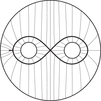
Figure 1: The figure 8, with a spike, as a boundary retract of the pair of pants. Each valence $k$ vertex is the endpoint of $k$ of the arcs $\gamma_{\eta}$.

Associated to $\Psi$ is the strong deformation retract $S\colon M\times[0,1]\rightarrow M$ of $M$ onto $E$ defined by $S(\Psi(\eta,s),t)=\Psi(\eta,s+t(1-s))$. The corresponding retraction $R\colon M\rightarrow E$ is defined by

$$R(\Psi(\eta,s))=\Psi(\eta,1).$$

If $E$ is a boundary retract of $M$ with associated retraction $R\colon M\rightarrow E$, then a continuous map $f\colon E\rightarrow E$ is said to unwrap in $M$ if there is a homeomorphism $\overline{f}\colon M\rightarrow M$ such that

1. $R\circ\overline{f}_{|E}=f$, and

2. There is some $k>0$ such that $\overline{f}^{k}$ is the identity on ${\partial}M$.

Such a homeomorphism $\overline{f}$ is called an unwrapping of $f$. A continuous family $\{f_{t}\}_{t\in I}$ in ${\mathcal{C}}(E,E)$ is said to unwrap in $M$ if it has a continuous family $\{\overline{f}_{t}\}_{t\in I}$ of unwrappings.

Finally, we say that $f\in{\mathcal{C}}(X,X)$ stabilizes at iterate $m$ if $f^{m+1}(X)=f^{m}(X)$ (there is no requirement for $m$ to be the least such integer). If $f$ stabilizes at iterate $m$ then

$${\varprojlim}(X,f)={\varprojlim}(f^{m}(X),f_{|f^{m}(X)}),$$

and the projection $\pi_{k}\colon{\varprojlim}(X,f)\to X$ has image $f^{m}(X)$ for all $k$.

The parameterized BBM construction can now be stated: the unparameterized version is obtained on taking the parameter space $I$ to be a point. Roughly speaking, the theorem states that a continuous family of continuous self-maps $f_{t}$ of $E$ which unwraps in $M$ and stabilizes at a common iterate gives rise to a continuous family of self-homeomorphisms $\Phi_{t}$ of $M$ having global attractors $\Lambda_{t}$ on which the dynamics of $\Phi_{t}$ is conjugate to that of $\hat{f}_{t}$. Moreover, the dynamics of $\Phi_{t}$ on $\Lambda_{t}$ is semi-conjugate to that of $f_{t}$ on $\bigcap_{k\geq 0}f_{t}^{k}(E)$ by a semi-conjugacy which can be extended to a continuous map $M\rightarrow M$ arbitrarily close to the identity; and the attactors $\Lambda_{t}\subset M$ vary continuously with $t$.

Theorem 3.1.

Let $M$ be a compact manifold with boundary ${\partial}M$, $E\subset M$ be a boundary retract of $M$, and $\{f_{t}\}_{t\in I}$ be a continuous family in ${\mathcal{C}}(E,E)$ which unwraps in $M$. Suppose moreover that there is some $m>0$ such that every $f_{t}$ stabilizes at iterate $m$. Then for each $\epsilon>0$ there is a continuous family $\{\Phi_{t}\}_{t\in I}$ in ${\mathcal{H}}(M,M)$ such that

1. For each $t\in I$ there is a compact $\Phi_{t}$-invariant subset $\Lambda_{t}$ of $M$ with the following properties:

   1. $\Phi_{t}|_{\Lambda_{t}}\colon\Lambda_{t}\rightarrow\Lambda_{t}$ is topologically conjugate to $\hat{f}_{t}\colon{\varprojlim}(E,f_{t})\rightarrow{\varprojlim}(E,f_{t})$.

   2. If $x\in M-{\partial}M$, the $\omega$-limit set $\omega(x,\Phi_{t})$ is contained in $\Lambda_{t}$.

   3. There is some $k>0$ such that each $\Phi_{t}^{k}$ is the identity on ${\partial}M$.

2. There is a continuous family $\{g_{t}\}_{t\in I}$ in ${\mathcal{C}}(M,M)$ with $d(g_{t},\operatorname{id})<\epsilon$, $g_{t}(\Lambda_{t})=f_{t}^{m}(E)$, and $f_{t}\circ g_{t}|_{\Lambda_{t}}=g_{t}\circ\Phi_{t}|_{\Lambda_{t}}$.

3. For each $t$, the semiconjugacy $g_{t}$ restricts to a bijection from the set of periodic points of $\Phi_{t}$ in $\Lambda_{t}$ to the set of periodic points of $f_{t}$.

4. The attractors $\Lambda_{t}$ vary Hausdorff continuously with $t\in I$.

Proof 3.2.

Let $\Psi\colon{\partial}M\times[0,1]\rightarrow M$ be the map expressing $E$ as a boundary retract of $M$. Let $\phi\colon[0,1]\rightarrow[0,1]$ be defined by $\phi(s)=2s$ for $s\in[0,1/2]$ and $\phi(s)=1$ for $s\in[1/2,1]$, and define $\Upsilon\colon M\rightarrow M$ by $\Upsilon(\Psi(\eta,s))=\Psi(\eta,\phi(s))$, which is well defined since $\phi(1)=1$. Because $\phi$ is the uniform limit of homeomorphisms $[0,1]\rightarrow[0,1]$, the map $\Upsilon$ is a near-homeomorphism.

Write $N(E)=\Psi(M\times[1/2,1])=\Upsilon^{-1}(E)$: thus $N(E)$ is a compact neighborhood of $E$ which is homeomorphic to $M$, by the homeomorphism $S\colon M\rightarrow N(E)$ defined by $S(\Psi(\eta,s))=\Psi(\eta,(s+1)/2)$.

Let $\{\overline{g}_{t}\}$ be the unwrapping of the family $\{f_{t}\}$, and define the family $\{\overline{f}_{t}\}$ in ${\mathcal{H}}(N(E),N(E))$ by $\overline{f}_{t}=S\circ\overline{g}_{t}\circ S^{-1}$. Extend $\{\overline{f}_{t}\}$ to a family in ${\mathcal{H}}(M,M)$ along the arc decomposition given by $\Psi$: that is, if $\lambda_{t}\colon{\partial}M\rightarrow{\partial}M$ is the homeomorphism defined by $\overline{f}_{t}(\Psi(\eta,1/2))=\Psi(\lambda_{t}(\eta),1/2)$, then $\overline{f}_{t}(\Psi(\eta,s))=\Psi(\lambda_{t}(\eta),s)$ for $s\in[0,1/2]$.

Now let $H_{t}=\Upsilon\circ\overline{f}_{t}\colon M\rightarrow M$ for each $t\in I$. Then $\{H_{t}\}$ is a near-isotopy, since $\Upsilon$ is a near-homeomorphism and each $\overline{f}_{t}$ is a homeomorphism. Moreover, for each $t\in I$ we have:

1. $H_{t}$ is equal to $f_{t}$ on $E$ (since $\Upsilon$ and $R$ restrict to the same retraction $\Psi(\eta,s)\mapsto\Psi(\eta,1)$ of $N(E)$ onto $E$, and $R\circ\overline{f}_{t}|_{E}=f_{t}$);

2. for all $x\in M-{\partial}M$, there is some $n\geq 0$ with $H_{t}^{n}(x)\in E$ (since $H_{t}(\Psi(\eta,s))=\Psi(\eta^{\prime},2s)$ for some $\eta^{\prime}$ if $s\leq 1/2$, and $H_{t}(\Psi(\eta,s))\in E$ if $s\geq 1/2$); and

3. there is some $k>0$ such that $H_{t}^{k}=\operatorname{id}$ on ${\partial}M$ (since $H_{t}=\overline{f}_{t}=\overline{g}_{t}$ on ${\partial}M$).

Let $h_{t}\colon M_{\infty}^{t}={\varprojlim}(M,H_{t})\rightarrow M$ be the homeomorphisms given by Corollary 2.4 (and constructed as in the proof of the corollary), so that $\{\Phi_{t}\}=\{h_{t}\circ\hat{H}_{t}\circ h_{t}^{-1}\}$ is a continuous family in ${\mathcal{H}}(M,M)$, and $d(h_{t},\pi_{0,t})<\epsilon$ for all $t$. We now show that (a), (b), (c), and (d) in the theorem statement hold for this family $\{\Phi_{t}\}$.

Property (a): By (I) above, there is a homeomorphic copy $\Omega_{t}$ of ${\varprojlim}(E,f_{t})$ embedded in $M_{\infty}^{t}$, namely

$$\Omega_{t}=\{{\underline{x}}\in M_{\infty}^{t}\,:\,x_{k}\in E\text{ for all }k\in{\mathbb{N}}\},$$

on which the restriction of $\hat{H}_{t}$ is topologically conjugate to $\hat{f}_{t}$. Hence $\Lambda_{t}=h_{t}(\Omega_{t})$ is a compact $\Phi_{t}$-invariant subset of $M$ with $\Phi_{t}|_{\Lambda_{t}}$ topologically conjugate to $\hat{f}_{t}\colon{\varprojlim}(E,f_{t})\rightarrow{\varprojlim}(E,f_{t})$.

By (II), $\omega({\underline{x}},\hat{H}_{t})\subset\Omega_{t}$ for all ${\underline{x}}\in M_{\infty}^{t}$ with $x_{0}\not\in{\partial}M$: that is, by the final statement of Corollary 2.4, for all ${\underline{x}}\not\in{\partial}M_{\infty}^{t}$. Hence $\omega(x,\Phi_{t})\subset\Lambda_{t}$ for all $x\not\in{\partial}M$. Similarly, (III) gives that $\hat{H}_{t}^{k}({\underline{x}})={\underline{x}}$ for all ${\underline{x}}\in M_{\infty}^{t}$ with $x_{0}\in{\partial}M$ (i.e. for all ${\underline{x}}\in{\partial}M_{\infty}^{t}$), from which it follows that $\Phi_{t}^{k}$ is the identity on ${\partial}M$.

Property (b): Let $g_{t}=\pi_{0,t}\circ h_{t}^{-1}\colon M\to M$: that is, using the notation of Theorem 2.2 and Corollary 2.4, $g_{t}(x)=y_{0}$, where $\beta^{-1}(x,t)=((y_{0},t),(y_{1},t),\ldots)$. It follows from the continuity of $\beta^{-1}$ that $\{g_{t}\}_{t\in I}$ is a continuous family in ${\mathcal{C}}(M,M)$. Moreover, $d(g_{t},\operatorname{id})<\epsilon$ for all $t$; and $g_{t}(\Lambda_{t})=g_{t}\circ h_{t}(\Omega_{t})=\pi_{0,t}(\Omega_{t})=f_{t}^{m}(E)$. Now

$$g_{t}\circ\Phi_{t}=\pi_{0,t}\circ\hat{H}_{t}\circ h_{t}^{-1}=H_{t}\circ\pi_{0,t}\circ h_{t}^{-1}=H_{t}\circ g_{t}\colon M\rightarrow M,$$

so that $g_{t}\circ\Phi_{t}|_{\Lambda_{t}}=f_{t}\circ g_{t}|_{\Lambda_{t}}$ by (I).

Property (c): This is an immediate consequence of the fact that $\pi_{0,t}$ restricts to a bijection from the set of periodic points of $\hat{H}_{t}$ to the set of periodic points of $H_{t}$, and $\operatorname{Per}(\Phi_{t})=h_{t}(\operatorname{Per}(\hat{H}_{t}))$.

Property (d): To show the Hausdorff continuity of $t\mapsto\Lambda_{t}$, we first show that the function $t\mapsto\Omega_{t}\subset M_{\infty}^{t}\subset M^{\mathbb{N}}$ is continuous as a function $I\rightarrow C(M^{\mathbb{N}})$ into the set of compact subsets of $M^{\mathbb{N}}$ with the Hausdorff metric. For this, it suffices to show that for all $\delta>0$ there is some $\eta>0$ such that if $d(s,t)<\eta$ then every point of $\Omega_{t}$ is within $\delta$ of a point of $\Omega_{s}$.

Recall that all of the $f_{t}$ stabilize at iterate $m$ so that $f_{t}\colon f_{t}^{m}(E)\rightarrow f_{t}^{m}(E)$ is surjective, and

$$\Omega_{t}=\{{\underline{x}}\in M_{\infty}^{t}\,:\,x_{k}\in f_{t}^{m}(E)\text{ for all }k\in{\mathbb{N}}\}.$$

Pick $J>1/\delta$ and $\eta>0$ such that

$$d(s,t)<\eta\implies d(f_{s}^{j},f_{t}^{j})<\delta\qquad\text{for }1\leq j<J+m$$ (3)

using the (uniform) continuity of $t\mapsto f_{t}^{j}$ for each $j$.

Let $s,t\in I$ with $d(s,t)<\eta$. Let ${\underline{x}}\in\Omega_{t}$, so that ${\underline{x}}=(x_{0},x_{1},x_{2},\ldots)$ with $x_{k}\in f_{t}^{m}(E)$ and $f_{t}(x_{k+1})=x_{k}$ for all $k$. Let $y\in E$ be such that $x_{J}=f_{t}^{m}(y)$. Define an element ${\underline{y}}=(y_{0},y_{1},y_{2},\ldots)$ of $(f_{s}^{m}(E))^{\mathbb{N}}$ by setting $y_{j}=f_{s}^{m}(f_{s}^{J-j}(y))$ for $0\leq j\leq J$, and then choosing $y_{j}\in f_{s}^{m}(E)$ for $j>J$ inductively to satisfy $f_{s}(y_{j})=y_{j-1}$.

Then ${\underline{y}}\in\Omega_{s}$, and $d({\underline{x}},{\underline{y}})<\delta$ as required, since

$$d(x_{j},y_{j})=d(f_{t}^{m+J-j}(y),f_{s}^{m+J-j}(y))<\delta\qquad\text{ for }0\leq j\leq J$$

by (3), and $1/(j+2)<\delta$ for $j>J$.

To complete the proof that $t\mapsto\Lambda_{t}$ is continuous, recall (using the notation of the proof of Corollary 2.4) that $\Lambda_{t}=h_{t}(\Omega_{t})=p_{1}\circ\beta\circ\iota_{t}(\Omega_{t})\subset M$. It is required to show that for all $\delta>0$ there is some $\eta>0$ such that, if $d(s,t)<\eta$, then every point of $\Lambda_{t}$ is within $\delta$ of a point of $\Lambda_{s}$. Now the map

$$K\colon\{({\underline{x}},t)\in M^{\mathbb{N}}\times I\,:\,{\underline{x}}\in\Omega_{t}\}\to(M\times I)_{\infty}$$

defined by $K({\underline{x}},t)=\iota_{t}({\underline{x}})$ is continuous, so we can pick $\xi>0$ such that if $d(({\underline{x}},t),({\underline{y}},s))<\xi$ then $d(p_{1}\circ\beta\circ K({\underline{x}},t),p_{1}\circ\beta\circ K({\underline{y}},s))<\delta$. By the first part of the proof, there is some $\eta>0$ such that if $d(s,t)<\eta$ and ${\underline{x}}\in\Omega_{t}$, then there is some ${\underline{y}}\in\Omega_{s}$ with $d(({\underline{x}},t),({\underline{y}},s))<\xi$.

Then, given $s,t\in I$ with $d(s,t)<\eta$ and $x\in\Lambda_{t}$, write $x=p_{1}\circ\beta\circ K({\underline{x}},t)$ for some ${\underline{x}}\in\Omega_{t}$. Let ${\underline{y}}\in\Omega_{s}$ with $d(({\underline{x}},t),({\underline{y}},s))<\xi$: then $y=p_{1}\circ\beta\circ K({\underline{y}},s)$ lies in $\Lambda_{s}$ with $d(x,y)<\delta$ as required.

1. The proof of part (a) of the theorem does not require the family to stabilize uniformly.

2. If condition (2) in the definition of an unwrapping is removed (so that an unwrapping $\overline{f}\in{\mathcal{H}}(M,M)$ is only required to satisfy $R\circ\overline{f}_{|E}=f$), then the theorem still holds except for part (a)(iii).

3. By part (a)(ii), if each boundary component of $M$ is collapsed to a point then each $\Phi_{t}$ becomes a homeomorphism of the resulting space (which in the surface case is a surface without boundary), for which every point except for a finite number of repelling periodic points has $\omega$-limit set contained in $\Lambda_{t}$.

4 Applications

4.1 Unimodal dynamics

The inverse limits of members of unimodal families of interval endomorphisms such as the tent family

$$T_{s}(x)=\min\{sx,s(1-x)\},\qquad 1\leq s\leq 2$$

and the quadratic family

$$f_{a}(x)=a-x^{2},\qquad-1/2\leq a\leq 2$$

have been intensively studied: a major recent advance is the proof by Barge, Bruin, and Štimac of Ingram’s conjecture, that if $1\leq t<s\leq 2$ then the inverse limits ${\varprojlim}(I,T_{t})$ and ${\varprojlim}(I,T_{s})$ are not homeomorphic (see [4] and the additional references therein).

Barge and Martin [6] showed that any map of the interval unwraps in the disk, and their construction gives a continuous family of unwrappings of any unimodal family. Thus Theorem 3.1 provides a continuously varying family $\Phi_{s}:D^{2}\rightarrow D^{2}$ of homeomorphisms of the disk, with $\Phi_{s}$ having ${\varprojlim}(I,T_{s})$ as a global attracting set. Moreover, since the family $T_{s}$ uniformly stabilizes at iterate one, these attractors vary continuously in the Hausdorff topology, although no two are homeomorphic. The family $\Phi_{s}$ has dynamics which increases monotonically with $s$: for example, the number of periodic orbits of each period increases with $s$, as does the topological entropy $h_{top}(\Phi_{s})=h_{top}(f_{s})=\log(s)$.

Extending the range of parameters to $s\in[0,2]$ illustrates the need for the stabilization hypothesis in Theorem 3.1. For $s\in[0,1)$ we have $T_{s}^{k}([0,1])\searrow\{0\}$ as $k\rightarrow\infty$, so these $T_{s}$ never stabilize and ${\varprojlim}(I,T_{s})$ is a point. On the other hand, $T_{1}$ is the identity on $T_{1}([0,1])=[0,1/2]$, so $T_{1}$ stabilizes at iterate 1 and ${\varprojlim}(I,T_{1})$ is an arc. Hence there is a discontinuous change in the attractor at $s=1$.

Theorem 3.1 may likewise be applied to the quadratic family, yielding a family of of plane homeomorphisms with monotonically increasing dynamics.

All of the constructions in this paper are strictly in the $C^{0}$-category. Embeddings of the inverse limits of members of the tent family as attractors of homeomorphisms with varying degrees of increased regularity have been carried out in [22, 24, 3, 11]. The fascinating question of which inverse limits and families of inverse limits can be embedded as attractors for $C^{r}$-diffeomorphisms is little understood. Barge and Holte [5] show that for certain parameter ranges the real Hénon attractor is conjugate to an inverse limit from the quadratic family. For example, for hyperbolic values of $a$ and small enough $b$, the Hénon map $H_{a,b}$ restricted to its attractor is conjugate to the inverse limit ${\varprojlim}(I,f_{a})$. As has been pointed out by several authors (for example [15, 16]), this cannot be extended to a uniform band of small values of $b$ in parameter space, since bifurcation curves for periodic orbits in the Hénon family cross arbitrarily close to $b=0$. In fact, the “antimonotonicity” results of [20] show that even if it were possible to embed the inverse limit of the unimodal family as a family of diffeomorphisms of the plane, it is not possible to do so with high regularity. Much of the work done to understand infinitely renormalizable Hénon maps [13, 21] is based on comparisons between them and the inverse limits of infinitely renormalizable unimodal maps.

The relationship of the inverse limit of the complex quadratic family to the complex Hénon family was used to great advantage in [17, 18]. More generally, the dynamics of families of homeomorphisms of ${\mathbb{R}}^{2}$ and ${\mathbb{C}}^{2}$ are often related to the inverse limits of 1-dimensional endomorphisms of graphs and (${\mathbb{R}}$-)trees and to branched surfaces (see [12]).

4.2 Rotation sets

If $\Phi\colon M\rightarrow M$ is a map of a compact, smooth manifold which acts as the identity on $H_{1}(M;{\mathbb{R}})$, one may define the rotation vector under $\Phi$ of a point $x\in M$. The usual way to do this is to lift $\Phi$ to $\tilde{\Phi}$ on the universal free Abelian cover $\tilde{M}_{A}$, and then use the lifts of a basis of closed one-forms to measure the average displacements of points ${\tilde{x}}\in\tilde{M}_{A}$ under $\tilde{\Phi}$ (see, for example, §3.3 of [8]). Because $\Phi$ acts as the identity on $H_{1}(M;{\mathbb{R}})$, $\tilde{\Phi}$ commutes with the deck transformations of $\tilde{M}_{A}$, and so the rotation vector is independent of the choice of lift ${\tilde{x}}\in\tilde{M}_{A}$ of a point $x\in M$. However, the rotation vector does depend in a simple way on the choice of lift $\tilde{\Phi}$. After fixing a lift $\tilde{\Phi}$ one defines the rotation set $\rho(\tilde{\Phi})$ (or $\rho(\Phi)$ if a lift is understood) as the collection of rotation vectors of points ${\tilde{x}}\in\tilde{M}_{A}$.

Now consider a self-map $f\colon E\rightarrow E$ of a boundary retract $E$ of $M$. Assume that $f$ acts as the identity on $H_{1}(E;{\mathbb{R}})$ and unwraps to a homeomorphism $\overline{f}\colon M\rightarrow M$ with $\overline{f}_{|{\partial}M}=\operatorname{id}$. Let $\Phi\colon M\rightarrow M$ be the BBM-extension homeomorphism obtained from Theorem 3.1 by taking the parameter space $I$ to be a point and $\epsilon<\operatorname{diam}(M)/10$. Since $E$ is a strong deformation retract of $M$, we also have that $\Phi_{*}=\operatorname{id}$ on $H_{1}(M;{\mathbb{R}})$. Thus both the rotation sets $\rho(\Phi)$ and $\rho(f)$ can be defined. They are essentially the same, provided that care is taken to choose corresponding lifts as will now be described.

By construction $\Phi_{|{\partial}M}=\operatorname{id}$, and we choose the lift $\tilde{\Phi}$ to $\tilde{M}_{A}$ which has $\tilde{\Phi}_{|{\partial}\tilde{M}_{A}}=\operatorname{id}$. Now we also lift the map $g\colon M\rightarrow M$ with $\tilde{d}(g,\operatorname{id})<\epsilon$ given by Theorem 3.1(b) to a $\tilde{g}\colon\tilde{M}_{A}\rightarrow\tilde{M}_{A}$ with $\tilde{d}(\tilde{g},\operatorname{id})<\epsilon$. If $\tilde{E}\subset\tilde{M}_{A}$ and $\tilde{\Lambda}\subset\tilde{M}_{A}$ are the lifts of $E$ and $\Lambda$ inside the universal free Abelian cover, we choose the lift $\tilde{f}\colon\tilde{E}\rightarrow\tilde{E}$ of $f$ so that $\tilde{f}\circ\tilde{g}({\tilde{z}})=\tilde{g}\circ\tilde{\Phi}({\tilde{z}})$ for all ${\tilde{z}}\in\tilde{\Lambda}$. Now the rotation set of a map is the same as its rotation set restricted to the recurrent set. Since by the BBM construction the recurrent set of $\Phi$ is contained in $\Lambda\cup{\partial}M$, we have $\rho(\tilde{\Phi})=\rho(\tilde{\Phi}_{|\tilde{\Lambda}})\cup\{0\}$. Finally, since $\tilde{d}(\tilde{g},\operatorname{id})<\epsilon$ we get that for any ${\tilde{z}}\in\tilde{\Lambda}$, $d(\tilde{\Phi}^{k}({\tilde{z}}),\tilde{f}^{k}(\tilde{g}({\tilde{z}})))<\epsilon$ for all $k\in{\mathbb{Z}}$. Thus since $\tilde{g}(\tilde{\Lambda})=\tilde{E}$, we have $\rho(\tilde{\Phi}_{|\tilde{\Lambda}})=\rho(\tilde{f})$, and so

$$\rho(\tilde{\Phi})=\rho(\tilde{f})\cup\{0\}.$$ (4)

By Theorem 3.1, (4) also holds for parameterized families and the attractors in the BBM-extension family vary continuously provided that the family stabilizes uniformly. An application is given in the authors’ forthcoming paper New rotation sets in a family of torus homeomorphisms, in which we consider a family of maps $k_{t}$ of the figure eight $E$ embedded as the spine of the two torus minus a disk. The resulting BBM-extension family is extended to a family of torus homeomorphisms $K_{t}$ as in Remark 3 (c). The intricate sequence of bifurcations of the rotation sets of the family $k_{t}$ can be described in detail using kneading theory techniques, and by (4) the rotation sets of the family $K_{t}$ of torus homeomorphisms undergo the same bifurcations.

4.3 The standard family of circle maps

The standard family of degree-one circle maps was introduced by Arnol’d [2]. This two-parameter family $f_{b,\omega}\colon S^{1}\rightarrow S^{1}$, for $b\geq 0$ and $0\leq\omega\leq 1$, is defined via its lifts $\tilde{f}_{b,\omega}\colon{\mathbb{R}}\rightarrow{\mathbb{R}}$, which are given by

$$\tilde{f}_{b,\omega}(x)=x+\omega+\frac{b}{2\pi}\sin(2\pi x).$$

The dynamics and bifurcations of this family have been much studied (see for example [7, 10, 23]). The main objects of interest in its parameter space are the so-called Arnol’d tongues $T_{r}$ given by

$$T_{r}=\{(b,\omega)\,:\,r\in\rho(f_{b,\omega})\}.$$

The core circle of an annulus $A$ is a boundary retract of $A$, and the family $f_{b,\omega}$ unwraps in $A$. Further, since each $f_{b,\omega}$ is onto, the family uniformly stabilizes at iterate zero. Thus, after restricting to the compact parameter space $b\in[0,b^{*}]$ for some large $b^{*}$, Theorem 3.1 yields a continuous family of annulus homeomorphisms $\Phi_{b,\omega}$ each having an attracting set $\Lambda_{b,\omega}$ homeomorphic to ${\varprojlim}(S^{1},f_{b,\omega})$ and, by (4), $\rho(\Phi_{b,\omega})=\rho(f_{b,\omega})\cup\{0\}$.

By composing each $\Phi_{b,\omega}$ with an appropriate lateral push on and near on the boundary we can obtain a new family of homeomorphisms $\Phi_{b,\omega}^{0}$ such that the rotation numbers of each $\Phi_{b,\omega}^{0}$ restricted to ${\partial}A$ are contained in $\rho(f_{b,\omega})$. We then have that

$$\rho(\Phi_{b,\omega}^{0})=\rho(f_{b,\omega})$$

for all $(b,\omega)\in[0,b^{*}]\times[0,1]$.

When $b\leq 1$, each $f_{b,\omega}$ is a homeomorphism and so the attractor of $\Phi_{b,\omega}^{0}$ is an invariant circle on which the dynamics is topologically conjugate to $f_{b,\omega}$. When $b>1$, however, the Arnol’d tongues $T_{r}$ for rational $r$ begin to overlap and for irrational $r$, $T_{r}$ opens from a Lipschitz curve into a tongue. These changes are accompanied by an elaborate sequence of bifurcations which are all shared by the family $\Phi_{b,\omega}^{0}$.

Philip Boyland
Department of Mathematics
University of Florida
372 Little Hall
Gainesville, FL 32611-8105, USA André de Carvalho
Departamento de Matemática Aplicada
IME-USP
Rua Do Matão 1010
Cidade Universitária
05508-090 São Paulo SP, Brazil Toby Hall
Department of Mathematical Sciences
University of Liverpool
Liverpool L69 7ZL, UK