Fast Distributed Computation in Dynamic Networks
via Random Walks

The paper investigates efficient distributed computation in dynamic networks in which the network topology changes (arbitrarily) from round to round. Random walks are a fundamental primitive in a wide variety of network applications; the local and lightweight nature of random walks is especially useful for providing uniform and efficient solutions to distributed control of dynamic networks. Given their applicability in dynamic networks, we focus on developing fast distributed algorithms for performing random walks in such networks.

Our first contribution is a rigorous framework for design and analysis of distributed random walk algorithms in dynamic networks. We then develop a fast distributed random walk based algorithm that runs in $\tilde{O}(\sqrt{\tau\Phi})$ rounds (with high probability), where $\tau$ is the dynamic mixing time and $\Phi$ is the dynamic diameter of the network respectively, and returns a sample close to a suitably defined stationary distribution of the dynamic network. We also apply our fast random walk algorithm to devise fast distributed algorithms for two key problems, namely, information dissemination and decentralized computation of spectral properties in a dynamic network.

Our next contribution is a fast distributed algorithm for the fundamental problem of information dissemination (also called as gossip) in a dynamic network. In gossip, or more generally, $k$-gossip, there are $k$ pieces of information (or tokens) that are initially present in some nodes and the problem is to disseminate the $k$ tokens to all nodes. We present a random-walk based algorithm that runs in $\tilde{O}(\min\{n^{1/3}k^{2/3}(\tau\Phi)^{1/3},nk\})$ rounds (with high probability). To the best of our knowledge, this is the first $o(nk)$-time fully-distributed token forwarding algorithm that improves over the previous-best $O(nk)$ round distributed algorithm [Kuhn et al., STOC 2010], although in an oblivious adversary model.

Our final contribution is a simple and fast distributed algorithm for estimating the dynamic mixing time and related spectral properties of the underlying dynamic network.

Keywords: Dynamic Network, Distributed Algorithm, Random walks, Random sampling, Information Dissemination, Gossip.

1 Introduction

Random walks play a central role in computer science spanning a wide range of areas in both theory and practice. Random walks are used as an integral subroutine in a wide variety of network applications ranging from token management and load balancing to search, routing, information propagation and gathering, network topology construction and building random spanning trees (e.g., see [12] and the references therein). They are particularly useful in providing uniform and efficient solutions to distributed control of dynamic networks [7, 29]. Random walks are local and lightweight and require little index or state maintenance which make them especially attractive to self-organizing dynamic networks such as peer-to-peer, overlay, and ad hoc wireless networks. In fact, in highly dynamic networks, where the topology can change arbitrarily from round to round (as assumed in this paper), extensive distributed algorithmic techniques that have been developed for the last few decades for static networks (see e.g., [27, 22, 28]) are not readily applicable. On the other hand, we would like distributed algorithms to work correctly and terminate even in networks that keep changing continuously over time (not assuming any eventual stabilization). Random walks being so simple and very local (each subsequent step in the walk depends only on the neighbors of the current node and does not depend on the topological changes taking place elsewhere in the network) can serve as a powerful tool to design distributed algorithms for such highly dynamic networks. However, it remains a challenge to show that one can indeed use random walks to solve non-trivial distributed computation problems efficiently in such networks, with provable guarantees. Our paper is a step in this direction.
A key purpose of random walks in many of the network applications is to perform node sampling. While the sampling requirements in different applications vary, whenever a true sample is required from a random walk of certain steps, typically all applications perform the walk naively — by simply passing a token from one node to its neighbor: thus to perform a random walk of length $\ell$ takes time linear in $\ell$. In prior work [12, 13], the problem of performing random walks in time that is significantly faster, i.e., sublinear in $\ell$, was studied. In [13], a fast distributed random walk algorithm was presented that ran in time sublinear in $\ell$, i.e., in $\tilde{O}(\sqrt{\ell D})$ rounds (where $D$ is the network diameter). This algorithm used only small sized messages (i.e., it assumed the standard CONGEST model of distributed computing [27]). However, a main drawback of this result is that it applied only to static networks. A major problem left open in [13] is whether a similar approach can be used to speed up random walks in dynamic networks.

The goals of this paper are two fold: (1) giving fast distributed algorithms for performing random walk sampling efficiently in dynamic networks, and (2) applying random walks as a key subroutine to solve non-trivial distributed computation problems in dynamic networks. Towards the first goal, we first present a rigorous framework for studying random walks in a dynamic network (cf. Section 2). (This is necessary, since it is not immediately obvious what the output of random walk sampling in a changing network means.) The main purpose of our random walk algorithm is to output a random sample close to the “stationary distribution” (defined precisely in Section 2) of the underlying dynamic network. Our random walk algorithms work under an oblivious adversary that fully controls the dynamic network topology, but does not know the random choices made by the algorithms (cf. Section 4 for a precise problem statements and results). We present a fast distributed random walk algorithm that runs in $\tilde{O}(\sqrt{\tau\Phi})$ with high probability (w.h.p.) , where $\tau$ is (an upper bound on) the dynamic mixing time and $\Phi$ is the dynamic diameter of the network respectively (cf. Section 6). Our algorithm uses small-sized messages only and returns a node sample that is “close” to the stationary distribution of the dynamic network (assuming the stationary distribution remains fixed even as the network changes). (The precise definitions of these terms are deferred to Section 2). We further extend our algorithm to efficiently perform and return $k$ independent random walk samples in $\tilde{O}(\min\{\sqrt{k\tau\Phi},k+\tau\})$ rounds (cf. Section 7). This is directly useful in the applications considered in this paper.

Towards the second goal, we present two main applications of our fast random walk sampling algorithm (cf. Section 8). The first key application is a fast distributed algorithm for the fundamental problem of information dissemination (also called as gossip) in a dynamic network. In gossip, or more generally, $k$-gossip, there are $k$ pieces of information (or tokens) that are initially present in some nodes and the problem is to disseminate the $k$ tokens to all nodes. In an $n$-node network, solving $n$-gossip allows nodes to distributively compute any computable function of their initial inputs using messages of size $O(\log n+d)$, where $d$ is the size of the input to the single node [19]. We present a random-walk based algorithm that runs in $\tilde{O}(\min\{n^{1/3}k^{2/3}(\tau\Phi)^{1/3},nk\})$ rounds with high probability (cf. Section 8.1). To the best of our knowledge, this is the first $o(nk)$-time fully-distributed token forwarding algorithm that improves over the previous-best $O(nk)$ round distributed algorithm [19], albeit under an oblivious adversarial model. A lower bound of $\Omega(nk/\log n)$ under the adaptive adversarial model of [19], was recently shown in [14]; hence one cannot do substantially better than the $O(nk)$ algorithm in general under an adaptive adversary.

Our second application is a decentralized algorithm for computing global metrics of the underlying dynamic network — dynamic mixing time and related spectral properties (cf. Section 8.2). Such algorithms can be useful building blocks in the design of topologically (self-)aware dynamic networks, i.e., networks that can monitor and regulate themselves in a decentralized fashion. For example, efficiently computing the mixing time or the spectral gap allows the network to monitor connectivity and expansion properties through time.

2 Network Model and Definitions

2.1 Dynamic Networks

We study a general model to describe a dynamic network with a fixed set of nodes. We consider an oblivious adversary which can make arbitrary changes to the graph topology in every round as long as the graph is connected. Such a dynamic graph process (or dynamic graph, for short) is also known as an Evolving Graph [3]. Suppose $V=\{v_{1},v_{2},\ldots,v_{n}\}$ be the set of nodes (vertices) and $\mathcal{G}=G_{1},G_{2},\ldots$ be an infinite sequence of undirected (connected) graphs on $V$. We write $G_{t}=(V,E_{t})$ where $E_{t}\in 2^{V\times V}$ is the dynamic edge set corresponding to round $t\in\mathbb{N}$. The adversary has complete control on the topology of the graph at each round, however it does not know the random choices made by the algorithm. In particular, in the context of random walks, we assume that it does not know the position of the random walk in any round (however, the adversary may know the starting position). Equivalently, we can assume that the adversary chooses the entire sequence $\langle G_{t}\rangle$ of the graph process $\mathcal{G}$ in advance before execution of the algorithm. This adversarial model has also been used in [3] in their study of random walks in dynamic networks.

We say that the dynamic graph process $\mathcal{G}$ has some property when each $G_{t}$ has that property. For technical reasons, we will assume that each graph $G_{t}$ is $d$-regular and non-bipartite. Later we will show that our results can be generalized to apply to non-regular graphs as well (albeit at the cost of a slower running time). The assumption on non-bipartiteness ensures that the mixing time is well defined, however this restriction can be removed using a standard technique: adding self-loops on each vertices (e.g., see [3]). Henceforth, we assume that the dynamic graph is a $d$-regular evolving graph unless otherwise stated (these two terms will be used interchangeably). Also we will assume that each $G_{t}$ is non-bipartite (and connected).

2.2 Distributed Computing Model

We model the communication network as an $n$-node dynamic graph process $\mathcal{G}=G_{1},G_{2},\ldots$. Every node has limited initial knowledge. Specifically, assume that each node is associated with a distinct identity number (id). (The node ids are of size $O(\log n)$.) At the beginning of the computation, each node $v$ accepts as input its own identity number and the identity numbers of its neighbors in $G_{1}$. The node may also accept some additional inputs as specified by the problem at hand (in particular, we assume that all nodes know $n$). The nodes are allowed to communicate through the edges of the graph $G_{t}$ in each round $t$. We assume that the communication occurs in synchronous rounds. In particular, all the nodes wake up simultaneously at the beginning of round $1$, and from this point on the nodes always know the number of the current round. We will use only small-sized messages. In particular, at the beginning of each round $t$, each node $v$ is allowed to send a message of size $B$ bits (typically $B$ is assumed to be $O(\operatorname{polylog}n)$) through each edge $e=(v,u)\in E_{t}$ that is adjacent to $v$. The message will arrive to $u$ at the end of the current round. This is a standard model of distributed computation known as the CONGEST(B) model [27, 25] and has been attracting a lot of research attention during last two decades (e.g., see [27] and the references therein). For the sake of simplifying our analysis, we assume that $B=O(\log^{2}n)$, although this is generalizable.

There are several measures of efficiency of distributed algorithms, but we will focus on one of them, specifically, the running time, i.e. the number of rounds of distributed communication. (Note that the computation that is performed by the nodes locally is “free”, i.e., it does not affect the number of rounds.)

2.3 Random Walks in a Dynamic Graph

Throughout, we assume the simple random walk in an undirected graph: In each step, the walk goes from the current node to a random neighbor, i.e., from the current node $v$, the probability to move in the next step to a neighbor $u$ is $\Pr(v,u)=1/d(v)$ for $(v,u)\in E$ and $0$ otherwise ($d(v)$ is the degree of $v$).

A simple random walk on dynamic graph $\mathcal{G}$ is defined as follows: assume that at time $t$ the walker is at node $v\in V$, and let $N(v)$ be the set of neighbors of $v$ in $G_{t}$, then the walker goes to one of its neighbors from $N(v)$ uniformly at random.

Suppose we have a random walk $v_{0}\rightarrow v_{1}\rightarrow\ldots\rightarrow v_{t}$ on a dynamic graph $\mathcal{G}$, where $v_{0}$ is the starting vertex. Then we get a probability distribution $P_{t}$ on $v_{t}$ starting from the initial distribution $P_{0}$ on $v_{0}$. We say that the distribution $P_{r}$ is stationary (or steady-state) for the graph process $\mathcal{G}$ if $P_{t+1}=P_{t}$ for all $t\geq r$. It is known that for every (undirected) static graph $G$, the distribution $\pi(v)=d(v)/2m$ is stationary. In particular, for a regular graph the stationary distribution is the uniform distribution. The mixing time of a random walk on a static graph $G$ is the time $t$ taken to reach “close” to the stationary distribution of the graph (see Definition 3.2 in Section 3 below). Similar to the static case, for a $d$-regular evolving graph, it is easy to verify that the stationary distribution is the uniform distribution. Also, for a $d$-regular evolving graph, the notion of dynamic mixing time (formally defined in Section 3) is similar to the static case and is well defined due to the monotonicity property of distributions (cf. Lemma 3.9 in Section 3). We show (cf. Theorem 3.6 in the next Section) that the dynamic mixing time is bounded by $O(\frac{1}{1-\lambda}\log n)$ rounds, where $\lambda$ is an upper bound of the second largest eigenvalue in absolute value of any graph in $\mathcal{G}$. Note that $O(\frac{1}{1-\lambda}\log n)$ is also an upper bound on the mixing time of the graph having $\lambda$ as its second largest eigenvalue and hence the dynamic mixing time is upper bounded by the worst-case mixing time of any graph in $\mathcal{G}$, which will be (henceforth) denoted by $\tau$. Since the second eigenvalue of the transition matrix of any regular graph is bounded by $1-1/n^{2}$ (cf. Corollary 3.8), this implies that $\tau$ of a $d$-regular evolving graph is bounded by $\tilde{O}(n^{2})$ (cf. Section 3). In general, the dynamic mixing time can be significantly smaller than this bound, e.g., when all graphs in $\mathcal{G}$ have $\lambda$ bounded from above by a constant (i.e., they are expanders — such dynamic graphs occur in applications e.g., [2, 19]), the dynamic mixing time is $O(\log n)$.

Another parameter affecting the efficiency of distributed computation in a dynamic graph is its dynamic diameter (also called flooding time, e.g., see [5, 9]). The dynamic diameter (denoted by $\Phi$) of an $n$-node dynamic graph $\mathcal{G}$ is the worst-case time (number of rounds) required to broadcast a piece of information from any given node to all $n$-nodes. The dynamic diameter can be much larger than the diameter ($D$) of any (individual) graph $G_{t}$.

3 Mixing Time of Regular Dynamic Graph

We have discussed the notion of random walk, probability distribution of a random walk , mixing time etc. on (dynamic) graph in Section 2.3 above. Here we formally define those notions.

Definition 3.1 (Distribution vector).

Let $\pi_{x}(t)$ define the probability distribution vector reached after $t$ steps when the initial distribution starts with probability $1$ at node $x$. Let $\pi$ denote the stationary distribution vector.

Definition 3.2.

[$\tau^{x}(\epsilon)$ ($\epsilon$-near mixing time for source $x$), $\tau^{x}_{mix}$ (mixing time for source $x$) and $\tau_{mix}$ (mixing time)] Define $\tau^{x}(\epsilon)=\min t:||\pi_{x}(t)-\pi||<\epsilon$. Define $\tau^{x}_{mix}=\tau^{x}(1/2e)$. Define $\tau_{mix}=\max_{x}\tau^{x}_{mix}$. ($\epsilon$ is a small constant).

We define the dynamic mixing time of a $d$-regular evolving graph $\mathcal{G}=G_{1},G_{2},\ldots$ as the maximum time taken for a simple random walk starting from any node to reach close to the uniform distribution on the vertex set. Therefore the definition of dynamic mixing time is similar to the static case. Let $\tau$ be the maximum mixing time of any (individual) graph $G_{t}$ in $\mathcal{G}$. (Note that $\tau$ is bounded by $\tilde{O}(n^{2})$ — follows from Theorem 3.6 and Corollary 3.8). We show that dynamic mixing time is well defined due to Theorem 3.6 and monotonicity property of distribution (cf. Section 3.1).

Definition 3.3.

[Dynamic mixing time] Define $\tau^{x}(\epsilon)$ ($\epsilon$-near mixing time for source $x$) is $\tau^{x}(\epsilon)=\min t:||\pi_{x}(t)-\pi||<\epsilon$. Note that $\pi_{x}(t)$ is the probability distribution on the graph $G_{t}$ in the dynamic graph process $\{G_{t}:t\geq 1\}$ when the initial distribution ($\pi_{x}(1)$) starts with probability $1$ at node $x$ on $G_{1}$. Define $\tau^{x}_{mix}$ (mixing time for source $x$) $=\tau^{x}(1/2e)$ and $\tau_{mix}=\max_{x}\tau^{x}_{mix}$. The dynamic mixing time is upper bounded by $\tau=\max\{$mixing time of all the static graph $G_{t}:t\geq 1\}$. Notice that $\tau\geq\tau_{mix}$ in general.

It is known that simple random walks on regular, connected, non-bipartite static graph have mixing time $O(\frac{\log n}{1-\lambda_{2}})$, where $\lambda_{2}$ is the second largest eigenvalue in absolute value of the graph. Interestingly, it turns out that similar result holds for $d$-regular, connected, non-bipartite evolving graphs. We show that the mixing time of a simple random walk on a dynamic graph $\mathcal{G}=G_{1},G_{2},\ldots$ is $O(\frac{\log n}{1-\lambda})$, where $\lambda$ is an upper bound of the second largest eigenvalue in absolute value of the graphs $\{G_{t}:t\geq 1\}$.

Lemma 3.4.

Let $G$ be an undirected connected non-bipartite $d$-regular graph on $n$ vertices and $p=(p_{1},\ldots,p_{n})$ be any probability distribution on its vertices. Let $A_{G}$ be the transition matrix of a simple random walk on $G$. Then,

$$\bigl{\|}pA_{G}-\frac{\textbf{1}}{n}\bigr{\|}\leq\bar{\lambda_{2}}\cdot\bigl{\|}p-\frac{\textbf{1}}{n}\bigr{\|}$$

where $\bar{\lambda_{2}}=\max_{i=2,\ldots,n}\lvert\lambda_{i}\rvert=\max\{\lambda_{2},-\lambda_{n}\}$ be the second largest eigenvalue in absolute value.

Proof.

Let $X_{1},X_{2},\ldots,X_{n}$ be an orthonormal set of eigenvectors of $A_{G}$ with corresponding eigenvalues $\lambda_{1}\geq\lambda_{2}\geq\ldots\geq\lambda_{n}$. Since $A_{G}$ is symmetric stochastic matrix, $\lambda_{1}=1$ and $X_{1}=\frac{\textbf{1}}{\sqrt{n}}$ and all eigenvectors and eigenvalues are real. Clearly,

$$\bigl{\|}pA_{G}-\frac{\textbf{1}}{n}\bigr{\|}=\bigl{\|}pA_{G}-\frac{\textbf{1}}{n}A_{G}\bigr{\|}=\bigl{\|}(p-\frac{\textbf{1}}{n})A_{G}\bigr{\|}$$

Since $p$ is a probability distribution, we can write it as $p=\beta_{1}X_{1}+\beta_{2}X_{2}+\ldots+\beta_{n}X_{n}$, where $\beta_{1},\beta_{2},\ldots,\beta_{n}\in\mathbb{R}$. Then $\beta_{1}=p\cdot X_{1}^{T}=\frac{1}{\sqrt{n}}\sum_{i}p_{i}=\frac{1}{\sqrt{n}}$, so that $\beta_{1}X_{1}=(\frac{1}{n},\frac{1}{n},\ldots,\frac{1}{n})$. Therefore, $p-\frac{\textbf{1}}{n}=\sum_{i=2}^{n}\beta_{i}X_{i}$. Hence,

$$\bigl{\|}p-\frac{\textbf{1}}{n}\bigr{\|}=\sqrt{\sum_{i=2}^{n}\beta_{i}^{2}}$$

Furthermore,

$$\bigl{\|}(p-\frac{\textbf{1}}{n})A_{G}\bigr{\|} =\bigl{\|}\sum_{i=2}^{n}\beta_{i}X_{i}A_{G}\bigr{\|}$$

$$=\bigl{\|}\sum_{i=2}^{n}\lambda_{i}\beta_{i}X_{i}\bigr{\|}$$

$$=\sqrt{\sum_{i=2}^{n}\lambda_{i}^{2}\beta_{i}^{2}}$$

$$\leq\max_{i=2,\ldots,n}|\lambda_{i}|\cdot\sqrt{\sum_{i=2}^{n}\beta_{i}^{2}}$$

$$=\bar{\lambda_{2}}\cdot\bigl{\|}p-\frac{\textbf{1}}{n}\bigr{\|}$$

Thus,

$$\bigl{\|}pA_{G}-\frac{\textbf{1}}{n}\bigr{\|}\leq\bar{\lambda_{2}}\cdot\bigl{\|}p-\frac{\textbf{1}}{n}\bigr{\|}$$

∎

An immediate corollary follows from the previous lemma:

Corollary 3.5.

Let $\mathcal{G}=G_{1},G_{2},\ldots$ be a sequence of undirected connected non-bipartite $d$-regular graphs on the same vertex set $V$. If $p_{0}$ is the initial probability distribution on $V$ and we perform a simple random walk on $\mathcal{G}$ starting from $p_{0}$, then the probability distribution $p_{t}$ of the walk after $t$ steps satisfies,

$$\bigl{\|}p_{t}-\frac{\textbf{1}}{n}\bigr{\|}\leq{\lambda}^{t}\bigl{\|}p_{0}-\frac{\textbf{1}}{n}\bigr{\|}$$

where $\lambda$ is an upper bound on the second largest eigenvalue in absolute value of the graphs $\{G_{t}:t\geq 1\}$.

Theorem 3.6.

For any $d$-regular connected non-bipartite evolving graph $\mathcal{G}$, the dynamic mixing time of a simple random walk on $\mathcal{G}$ is bounded by $O(\frac{1}{1-{\lambda}}\log n)$, where $\lambda$ is an upper bound of the second largest eigenvalue in absolute value of any graph in $\mathcal{G}$.

Proof.

Let the random walk starts from a given vertex with distribution $p_{0}=(1,0,\ldots,0)$. From Corollary 3.5 and the fact that $\bigl{\|}p_{0}-\frac{\textbf{1}}{n}\bigr{\|}=O(1)$ we have,

$$\bigl{\|}p_{t}-\frac{\textbf{1}}{n}\bigr{\|}\leq{\lambda}^{t}$$

So for $t=O(\frac{1}{1-{\lambda}}\log n)$ gives $\bigl{\|}p_{t}-\frac{\textbf{1}}{n}\bigr{\|}\leq\frac{1}{n^{O(1)}}$. ∎

Lemma 3.7.

Let $G$ be an undirected connected $d$-regular graph on $n$ vertices. Let $A_{G}$ be the transition matrix of $G$. If $\lambda_{1}\geq\lambda_{2}\geq\ldots\geq\lambda_{n}$ are the eigenvalues of $A_{G}$, then $\lambda_{1}=1$ and for $i\geq 2,\lambda_{i}\leq 1-\frac{1}{dDn}$, where $D$ is the diameter of the graph.

Proof.

The normalized eigenvector corresponding to $\lambda_{1}=1$ is $X_{1}=\frac{1}{\sqrt{n}}(1,1,\ldots,1)$. Consider any normalized real eigenvector $X\perp X_{1}$ with its eigenvalue $\lambda$. Hence, $\sum_{i=1}^{n}x_{i}^{2}=1$ and $\sum_{i=1}^{n}x_{i}=0$, where $X=(x_{1},x_{2},\ldots,x_{n})$. Let $x_{t}$ and $x_{s}$ be the respectively largest and smallest co-ordinates of $X$. Clearly $x_{t}\geq 1/\sqrt{n}$ and $x_{s}<0$. Let $s=v_{1}\to v_{2}\to\ldots\to v_{k}=t$ be the vertices on a shortest path from $s$ to $t$ in $G$. Consider $X(\mathbb{I}-A_{G})X^{T}$. Then,

$$1-\lambda =X(\mathbb{I}-A_{G})X^{T}=\frac{1}{d}\cdot\sum_{\{i,j\}\in E(G)}(x_{i}-x_{j})^{2}$$

$$\geq\frac{1}{d}\cdot\sum_{i=1}^{k-1}(x_{v_{i}}-x_{v_{i+1}})^{2}$$

$$\geq\frac{1}{d(k-1)}\cdot\left(\sum_{i=1}^{k-1}x_{v_{i}}-x_{v_{i+1}}\right) [\text{by Cauchy-Schwarz inequality}]$$

$$=\frac{1}{d(k-1)}\cdot(x_{s}-x_{t})^{2}$$

$$\geq\frac{1}{dDn}$$

where $k-1\leq D$, the diameter of the graph. ∎

Corollary 3.8.

$(1-\frac{1}{n^{2}})$ is an upper bound of the second largest eigenvalue $\bar{\lambda_{2}}$ of the transition matrix of any undirected connected regular graph on $n$-vertices.

Proof.

This follows from the Lemma 3.7 and the fact that the diameter of any connected regular graph is bounded by $O(\frac{n}{d})$. ∎

3.1 Monotonicity property of the distribution vector

Let $\pi_{x}(t)$ define the probability distribution vector of a simple random walk reached after $t$ steps when the initial distribution starts with probability $1$ at node $x$. Let $\pi$ denote the stationary distribution vector. We show in the following lemma that the vector $\pi_{x}(t)$ gets closer to $\pi$ as $t$ increases.

Lemma 3.9.

$||\pi_{x}(t+1)-\pi||\leq||\pi_{x}(t)-\pi||$.

Proof.

We need to show that the definition of mixing times are consistent, i.e. monotonic in $t$, the walk length of the random walk. Let $A$ be the transition matrix of a simple random walk on a $d$-regular evolving graph $\mathcal{G}$ which in fact changes from round to round. The entries $a_{ij}$ of $A$ denotes the probability of transitioning from node $i$ to node $j$. The monotonicity follows from the fact that for any transition matrix $A$ of any regular graph and for any probability distribution vector $p$,

$$||(p-\frac{\mathbf{1}}{n})A||<||p-\frac{\mathbf{1}}{n}||.$$

This result follows from the above Lemma 3.4 and the fact that $\bar{\lambda_{2}}<1$.

Let $\pi$ be the stationary distribution of the matrix $A$. Then $\pi=(\frac{1}{n},\frac{1}{n},\ldots,\frac{1}{n})$. This implies that if $t$ is $\epsilon$-near mixing time, then $||pA^{t}-\pi||\leq\epsilon$, by definition of $\epsilon$-near mixing time. Now consider $||pA^{t+1}-\pi||$. This is equal to $||pA^{t+1}-\pi A||$ since $\pi A=\pi$. However, this reduces to $||(pA^{t}-\pi)A||<||pA^{t}-\pi||\leq\epsilon$. It follows that $(t+1)$ is $\epsilon$-near mixing time and $||pA^{t+1}-\pi||<||pA^{t}-\pi||$. ∎

4 Problem Statements and Our Results

We formally state the problems and our main results.

The Single Random Walk problem.

Given a $d$-regular evolving graph $\mathcal{G}=(V,E_{t})$ and a starting node $s\in V$, our goal is to devise a fast distributed random walk algorithm such that, at the end, a destination node, sampled from a $\tau$-length walk, outputs the source node’s ID (equivalenty, one can require $s$ to output the destination node’s ID), where $\tau$ is (an upper bound on) the dynamic mixing time of $\mathcal{G}$ (cf. Section 3), under the assumption that $\mathcal{G}$ is modified by an oblivious adversary (cf. Section 2). Note that this distribution will be “close” to the stationary distribution of $\mathcal{G}$ (stationary distribution and $\tau$ are both well-defined — cf. Section 3). Since we are assuming a $d$-regular evolving graph, our goal is to sample from (or close to) the uniform distribution (which is the stationary distribution) using as few rounds as possible. Note that we would like to sample fast via random walk — this is also very important for the applications considered in this paper. On the other hand, if one had to simply get a uniform random sample, it can be accomplished by other means, e.g., it is easy to obtain it in $O(\Phi)$ rounds (by using flooding).

For clarity, observe that the following naive algorithm solves the above problem in $O(\tau)$ rounds: The walk of length $\tau$ is performed by sending a token for $\tau$ steps, picking a random neighbor in each step. Then, the destination node $v$ of this walk outputs the ID of $s$. Our goal is to perform such sampling with significantly less number of rounds, i.e., in time that is sublinear in $\tau$, in the CONGEST model, and using random walks rather than naive flooding techniques. As mentioned earlier this is needed for the applications discussed in this paper. Our result is as follows.

Theorem 4.1.

The algorithm Single-Random-walk (cf. Algorithm 1) solves the Single Random Walk problem in a dynamic graph and with high probability finishes in $\tilde{O}(\sqrt{\tau\Phi})$ rounds.

The above algorithm assumes that nodes have knowledge of $\tau$ (or at least some good estimate of it). (In many applications, it is easy to have a good estimate of $\tau$ when there is knowledge of the structure of the individual graphs — e.g., each $G_{t}$ is an expanders as in [2, 26].) Notice that in the worst case the value of $\tau$ is $\tilde{\Theta}(n^{2})$, and hence this bound can be used even if nodes have no knowledge. Therefore putting $\tau=\tilde{\Theta}(n^{2})$ in the above Theorem 4.1, we see that our algorithm samples a node from the uniform distribution through a random walk in $\tilde{O}(n\sqrt{\Phi})$ rounds w.h.p. Our algorithm can also be generalized to work for non-regular evolving graphs also (cf. Section 6.3).

We also consider the following extension of the Single Random Walk problem, called the $k$ Random Walks problem: We have $k$ sources $s_{1},s_{2},...,s_{k}$ (not necessarily distinct) and we want each of the $k$ destinations to output an ID of its corresponding source, assuming that each source initiates an independent random walk of length $\tau$. (Equivalently, one can ask each source to output the ID of its corresponding destination.) The goal is to output all the ID’s in as few rounds as possible. We show that:

Theorem 4.2.

The algorithm Many-Random-Walks (cf. Algorithm 2) solves the $k$ Random Walks problem in a dynamic graph and with high probability finishes in $\tilde{O}\left(\min(\sqrt{k\tau\Phi},k+\tau)\right)$ rounds.

Information dissemination (or $k$-gossip) problem.

In $k$-gossip, initially $k$ different tokens are assigned to a set $V$ of $n(\geq k)$ nodes. A node may have more than one token. The goal is to disseminate all the $k$ tokens to all the $n$ nodes. We present a fast distributed randomized algorithm for $k$-gossip in a dynamic network. Our algorithm uses Many-Random-Walks as a key subroutine; to the best of our knowledge, this is the first subquadratic time fully-distributed token forwarding algorithm.

Theorem 4.3.

The algorithm K-Information-Dissemination (cf. Algorithm 3) solves $k$-gossip problem in a dynamic graph with high probability in $\tilde{O}(\min\{n^{1/3}k^{2/3}(\tau\Phi)^{1/3},nk\})$ rounds.

Mixing time estimation.

Given a dynamic network, we are interested in (approximately) computing the dynamic mixing time, assuming that the mixing time of the (individual) graphs do not change. We present an efficient distributed algorithm for estimating the mixing time. In particular, we show the following result where $\tau^{x}_{mix}$ is the dynamic mixing time with respect to a starting node $x$. We formally define these notions in Section 3. This gives an alternative algorithm to the only previously known approach by Kempe and McSherry [18] that can be used to estimate $\tau^{x}_{mix}$ in a static graph in $\tilde{O}(\tau^{x}_{mix})$ rounds.

Theorem 4.4.

Given connected $d$-regular evolving graphs with dynamic diameter $\Phi$, a node $x$ can find, in $\tilde{O}(n^{1/4}\sqrt{\Phi\tau^{x}(\epsilon)})$ rounds, a time $\tilde{\tau}^{x}_{mix}$ such that $\tau^{x}_{mix}\leq\tilde{\tau}^{x}_{mix}\leq\tau^{x}(\epsilon)$, where $\epsilon=\frac{1}{6912e\sqrt{n}\log n}$.

5 Related Work and Technical Overview

Dynamic networks.

As a step towards understanding the fundamental computational power in dynamic networks, recent studies (see e.g., [8, 19, 20, 14] and the references therein) have investigated dynamic networks in which the network topology changes arbitrarily from round to round. In the worst-case model that was studied by Kuhn, Lynch, and Oshman [19], the communication links for each round are chosen by an online adversary, and nodes do not know who their neighbors for the current round are before they broadcast their messages. Unlike prior models on dynamic networks, the model of [19] (like ours) does not assume that the network eventually stops changing; therefore it requires that the algorithms work correctly and terminate even in networks that change continually over time.

The work of [3] studied the cover time of random walks in an evolving graph (cf. Section 2) in an oblivious adversarial model. In a regular evolving graph, they show that the cover time is always polynomial, while this is not true in general if the graph is not regular — the cover time can be exponential. However, they show that a lazy random walk (i.e., walk with self loops) has polynomial cover time on all graphs. We also use a similar strategy to show that our distributed random walk algorithms can work on non-regular graphs also, albeit at the cost of an increase in run time. While the work of [3] addressed the cover time of random walks on dynamic graphs, this paper is concerned with distributed algorithms for computing random walk samples fast with the goal towards applying it to fast distributed computation problems in dynamic networks.

Recently, the work of [10], studies the flooding time of Markovian evolving dynamic graphs, a special class of evolving graphs.

Distributed random walks.

Our fast distributed random walk algorithms are based on previous such algorithms designed for static networks [12, 13]. These were the first sublinear (in the length of the walk) time algorithms for performing random walks in graphs. The algorithm of [13] performed a random walk of length $\ell$ in $\tilde{O}(\sqrt{\ell D})$ rounds (with high probability) on an undirected network, where $D$ is the diameter of the network. (Subsequently, the algorithm of [13] was shown to be almost time-optimal (up to polylogarithmic factors) in [24].) The general high-level idea of the above algorithm is using a few short walks in the beginning (executed in parallel) and then carefully concatenating these walks together later as necessary. A main contribution of the present work is showing that building on the approach of [13] yields speed up in random walk computations even in dynamic networks. However, there are some challenging technical issues to overcome in this extension given the continuous dynamic nature (cf. Section 6). One key technical lemma (called the Random walk visits Lemma) that was used to show the almost-optimal run time of $\tilde{O}(\sqrt{\ell D})$ does not directly apply to dynamic networks. In the static setting, this lemma gives a bound on the number of times any node is visited in an $\ell$-length walk, for any length that is not much larger than the cover time. More precisely, the lemma states that w.h.p. any node $x$ is visited at most $\tilde{O}(d(x)\sqrt{\ell})$ times, in an $\ell$-length walk from any starting node ($d(x)$ is the degree of $x$). In this paper, we show that a similar bound applies to an $\ell$-length random walk on any $d$-regular evolving graph (cf. Lemma 6.4). A key ingredient in the above proof is showing that a technical result due to Lyons [23] can be made to work on an evolving graph.

Other recent work involving multiple random walks in static networks, but in different settings include Alon et. al. [1], Elsässer et. al. [6], and Cooper et al. [11].

Information spreading.

The main application of our random walks algorithm is an improved algorithm for information spreading or gossip in dynamic networks. To the best of our knowledge, it gives the first subquadratic, fully distributed, token forwarding algorithm in dynamic networks, partially answering an open question raised in [14]. Information spreading is a fundamental primitive in networks which has been extensively studied (see e.g., [14] and the references therein). Information spreading can be used to solve other problems such as broadcasting and leader election.

This paper’s focus is on token-forwarding algorithms, which do not manipulate tokens in any way other than storing and forwarding them. Token-forwarding algorithms are simple, often easy to implement, and typically incur low overhead. [19] showed that under their adversarial model, $k$-gossip can be solved by token-forwarding in $O(nk)$ rounds, but that any deterministic online token-forwarding algorithm needs $\Omega(n\log k)$ rounds. In [14], an almost matching lower bound of $\Omega(nk/\log n)$ is shown. The above lower bound indicates that one cannot obtain efficient (i.e., subquadratic) token-forwarding algorithms for gossip in the adversarial model of [19]. This motivates considering other weaker (and perhaps more realistic) models of dynamic networks.

[14] presented a polynomial-time offline centralized token-forwarding algorithm that solves the $k$-gossip problem on an $n$-node dynamic network in $O(\min\{nk,n\sqrt{k\log n}\})$ rounds with high probability. This is the first known subquadratic time token-forwarding algorithm but it is not distributed, and furthermore, the centralized algorithm needs to know the complete evolution of the dynamic graph in advance. It was left open in [14] whether one can obtain a fully-distributed and localized algorithm that also does not know anything about how the network evolves. In this paper, we resolve this open question in the affirmative. Our algorithm runs in $\tilde{O}(\min\{n^{1/3}k^{2/3}(\tau\Phi)^{1/3},nk\})$ rounds with high probability. This is significantly faster than the $O(nk)$-round algorithm of [19] as well as the above centralized algorithm of [14] when $\tau$ and $\Phi$ are not too large. Note that $\Phi$ is bounded by $O(n)$ and in regular graphs $\tau$ is $O(n^{2})$ ($O(n^{3})$ in general graphs) and so in general, our bounds cannot be better than $O(nk)$.

We note that an alternative approach based on network coding was due to  [15, 16], which achieves an $O(nk/\log n)$ rounds using $O(\log n)$-bit messages (which is not significantly better than the $O(nk)$ bound using token-forwarding), and $O(n+k)$ rounds with large message sizes (e.g., $\Theta(n\log n)$ bits). It thus follows that for large token and message sizes there is a factor $\Omega(\min\{n,k\}/\log n)$ gap between token-forwarding and network coding. We note that in our model we allow only one token per edge per round and thus our bounds hold regardless of the token size.

6 Algorithm for Single Random Walk

6.1 Description of the Algorithm

We develop an algorithm called Single-Random-Walk (cf. Algorithm 1) for $d$-regular evolving graph ($\mathcal{G}=(V,E_{t})$). The algorithm performs a random walk of length $\tau$ (the dynamic mixing time of $\mathcal{G}$ — cf. Section 2.3) in order to sample a destination from (close to) the uniform distribution on the vertex set $V$.

The high-level idea of the algorithm is to perform “many” short random walks in parallel and later “stitch” the short walks to get the desired walk of length $\tau$. In particular, we perform the algorithm in two phases, as follows. For simplicity we call the messages used in Phase 1 as “coupons” and in Phase 2 as “tokens”. In Phase 1, we perform $d$ (degree of the graph) “short” (independent) random walks of length $\lambda$ (to bound the running time correctly, we show later that we do short walks of length approximately $\lambda$, instead of $\lambda$) from each node $v$, where $\lambda$ is a parameter whose value will be fixed in the analysis. This is done simply by forwarding $d$ “coupons” having the ID of $v$ from $v$ (for each node $v$) for $\lambda$ steps via random walks.

In Phase 2, starting at source $s$, we “stitch” (see Figure 1) some of short walks prepared in Phase 1 together to form a longer walk. The algorithm starts from $s$ and randomly picks one coupon distributed from $s$ in Phase 1. We now discuss how to sample one such coupon randomly and go to the destination vertex of that coupon. This can be done easily as follows: In the beginning of Phase 1, each node $v$ assigns a coupon number for each of its $d$ coupons. At the end of Phase 1, the coupons originating at $s$ (containing ID of $s$ plus a coupon number) are distributed throughout the network (after Phase 1). When a coupon needs to be sampled, node $s$ chooses a random coupon number (from the unused set of coupons) and informs the destination node (which will be the next stitching point) holding the coupon $C$ through flooding. Let $C$ be the sampled coupon and $v$ be the destination node of $C$. $s$ then sends a “token” to $v$ (through flooding) and $s$ deletes coupon $C$ (so that $C$ will not be sampled again next time at $s$, otherwise, randomness will be destroyed). The process then repeats. That is, the node $v$ currently holding the token samples one of the coupons it distributed in Phase 1 and forwards the token to the destination of the sampled coupon, say $v^{\prime}$. Nodes $v,v^{\prime}$ are called “connectors” - they are the endpoints of the short walks that are stitched. A crucial observation is that the walk of length $\lambda$ used to distribute the corresponding coupons from $s$ to $v$ and from $v$ to $v^{\prime}$ are independent random walks. Therefore, we can stitch them to get a random walk of length $2\lambda$. We therefore can generate a random walk of length $3\lambda,4\lambda,\ldots$ by repeating this process. We do this until we have completed more than $\tau-\lambda$ steps. Then, we complete the rest of the walk by doing the naive random walk algorithm.

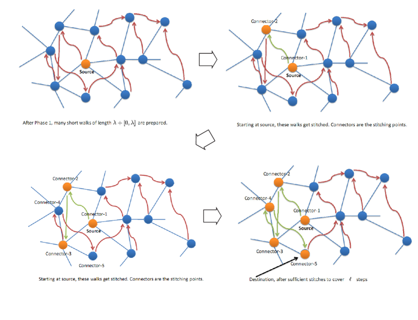
Figure 1: Figure illustrating the Algorithm of stitching short walks together.

To understand the intuition behind this algorithm, let us analyze its running time. First, we claim that Phase 1 needs $O(\lambda)$(see Lemma 6.2) rounds with high probability. Recall that, in Phase 1, each node prepares $d$ independent random walks of length $\lambda$ (approximately). We start with $d=\deg(v)$ coupons from each node $v$ at the same time, each edge in the current graph should receive two coupons in the average case. In other words, there is essentially no congestion (i.e., not too many coupons are sent through the same edge). Therefore sending out (just) $d$ coupons from each node for $\lambda$ steps will take $O(\lambda)$ rounds in expectation. This argument can be modified to show that we need $O(\lambda)$ rounds with high probability in our model (see full proof of the Lemma 6.2). Now by the definition of dynamic diameter, flooding takes $\Phi$ rounds. We show that sample a coupon can be done in $O(\Phi)$ rounds (cf. Lemma 6.3) and it follows that Phase 2 needs $\tilde{O}(\Phi\cdot\tau/\lambda)$ rounds. Therefore, the algorithm needs $\tilde{O}(\lambda+\Phi\cdot\tau/\lambda)$ which is $\tilde{O}(\sqrt{\tau\Phi})$ when we set $\lambda=\sqrt{\tau\Phi}$.

The reason the above algorithm for Phase 2 is incomplete is that it is possible that $d$ coupons are not enough: We might forward the token to some node $v$ many times in Phase 2 and all coupons distributed by $v$ in the first phase are deleted. (In other words, $v$ is chosen as a connector node many times, and all its coupons have been exhausted.) If this happens then the stitching process cannot progress. To fix this problem, we will show (in the next section) an important property of the random walk which says that a random walk of length $O(\tau)$ will visit each node $v$ at most $\tilde{O}(\sqrt{\tau}d)$ times (cf. Lemma 6.4). But this bound is not enough to get the desired running time, as it does not say anything about the distribution of the connector nodes. We use the following idea to overcome it: Instead of nodes performing walks of length $\lambda$, each such walk $i$ do a walk of length $\lambda+r_{i}$ where $r_{i}$ is a random number in the range $[0,\lambda-1]$. Since the random numbers are independent for each walk, each short walks are now of a random length in the range $[\lambda,2\lambda-1]$. This modification is needed to claim that each node will be visited as a connector only $\tilde{O}(\sqrt{\tau}d/\lambda)$ times (cf. Lemma 6.12). This implies that each node does not have to prepare too many short walks. It turns out that this aspect requires quite a bit more work in the dynamic setting and therefore needs new ideas and techniques. The compact pseudo code is given in Algorithm 1.

Algorithm 1 Single-Random-Walk($s$, $\tau$)

Input: Starting node $s$, desired walk length $\tau$ and parameter $\lambda$.
Output: Destination node of the walk outputs the ID of $s$.

Phase 1: (Each node $v$ performs $d=\deg(v)$ random walks of length $\lambda+r_{i}$ where $r_{i}$ (for each $1\leq i\leq d$) is chosen independently at random in the range $[0,\lambda-1]$. At the end of the process, there are $d$ (not necessarily distinct) nodes holding a “coupon” containing the ID of v.)

1:  for each node $v$ do

2:     Generate $d$ random integers in the range $[0,\lambda-1]$, denoted by $r_{1},r_{2},\ldots,r_{d}$.

3:     Construct $d$ messages containing its ID, a counter number and in addition, the $i$-th message contains the desired walk length of $\lambda+r_{i}$. We will refer to these messages created by node $v$ as “coupons created by $v$”.

4:  end for

5:  for $i=1$ to $2\lambda$ do

6:     This is the $i$-th round. Each node $v$ does the following: Consider each coupon $C$ held by $v$ which is received in the $(i-1)$-th round. If the coupon $C$’s desired walk length is at most $i$, then $v$ keeps this coupon ($v$ is the desired destination). Else, $v$ picks a neighbor $u$ uniformly at random for each coupon $C$ and forward $C$ to $u$.

7:  end for

Phase 2: (Stitch short walks by token forwarding. Stitch $\Theta(\tau/\lambda)$ walks, each of length in $[\lambda,2\lambda-1]$.)

1:  The source node $s$ creates a message called “token” which contains the ID of $s$

2:  The algorithm will forward the token around and keep track of a set of connectors, denoted by $C$. Initially, $C=\{s\}$

3:  while Length of walk completed is at most $\tau-2\lambda$ do

4:     Let $v$ be the node that is currently holding the token.

5:     $v$ sample one of the coupons distributed by $v$ uniformly at random (by randomly chosen one counter number from the unused set of coupons). Let $v^{\prime}$ be the destination node of the sampled coupon, say $C$.

6:     $v$ sends the token to $v^{\prime}$ through broadcast and delete the coupon $C$.

7:     $C=C\cup\{v\}$

8:  end while

9:  Walk naively until $\tau$ steps are completed (this is at most another $2\lambda$ steps)

10:  A node holding the token outputs the ID of $s$

6.2 Analysis

We first show the correctness of the algorithm and then analyze the time complexity.

6.2.1 Correctness

Lemma 6.1.

The algorithm Single-Random-Walk, with high probability, outputs a node sample that is close to the uniform probability distribution on the vertex set $V$.

Proof.

(sketch) We know (from Theorem 3.6) that any random walk on a regular evolving graph reaches “close” to the uniform distribution at step $\tau$ regardless of any changes of the graph in each round as long as it is $d$-regular, non-bipartite and connected. Therefore it is sufficient to show that Single-Random-Walk finishes with a node $v$ which is the destination of a true random walk of length $\tau$ on some appropriate dynamic graph from the source node $s$. We show this below in two steps.
First we show that each short walk (of length approximately $\lambda$) created in phase 1 is a true random walk on a dynamic graph sequence $G_{1},G_{2},\ldots,G_{\tilde{\lambda}}$ ($\tilde{\lambda}$ is some approximate value of $\lambda$). This means that in every step $t$, each walk moves to some random neighbor from the current node on the graph $G_{t}$ and each walk is independent of others. The proof of the Lemma 6.2 shows that w.h.p there is at most $O(\log^{2}n)$ bits congestion in any edge in any round in Phase 1. Since we consider CONGEST($\log^{2}n$) model, at each round $O(\log^{2}n)$ bits can be sent through each edge from each direction. Hence effectively there will be no delay in Phase 1 and all walks can extend their length from $i$ to $i+1$ in one round. Clearly each walk is independent of others as every node sends messages independently in parallel. This proves that each short walk (of a random length in the range $[\lambda,2\lambda-1]$) is a true random walk on the graph $G_{1},G_{2},\ldots,G_{\tilde{\lambda}}$.
In Phase 2, we stitch short walks to get a long walk of length $\tau$. Therefore, the $\tau$-length random walk is not from the dynamic graph sequence $G_{1},G_{2},\ldots,G_{\tau}$; rather it is from the sequence:
$G_{1},G_{2},\ldots,G_{\tilde{\lambda}},G_{1},G_{2},\ldots,G_{\tilde{\lambda}},\ldots,$ ($\tau/\lambda$ times approximately). The stitching part is done on the graph sequence from $G_{\tilde{\lambda}+1},G_{\tilde{\lambda}+2},\ldots$ onwards. This does not affect the distribution of probability on the vertex set in each step, since the graph sequence from $G_{\tilde{\lambda}+1},G_{\tilde{\lambda}+2},\ldots$ is used only for communication. Also note that since we define $\tau$ to be the maximum of any static graph $G_{t}$’s mixing time, it clearly reaches close to the uniform distribution after $\tau$ steps of walk in the graph sequence $G_{1},G_{2},\ldots,G_{\tilde{\lambda}},G_{1},G_{2},\ldots,G_{\tilde{\lambda}},\ldots,$ ($\tau/\lambda$ times approximately).
Finally, when we stitch at a node $v$, we are sampling a coupon (short walk) uniformly at random among many coupons (and therefore, short walks starting at $v$) distributed by $v$. It is easy to see that this stitches short random walks independently and hence gives a true random walk of longer length. Thus it follows that the algorithm Single-Random-Walk returns a destination node of a $\tau$-length random walk (starting from $s$) on some evolving graph. ∎

6.2.2 Time Analysis

We show the running time of algorithm Single-Random-Walk (cf. Theorem 4.1) using the following lemmas.

Lemma 6.2.

Phase 1 finishes in $O(\lambda)$ rounds with high probability.

Proof.

In phase 1, each node $v$ performs $d$ walks of length $\lambda$. Initially all the node starts with $d$ coupons (or messages) and each coupon takes a random walk. We prove that after any given number of steps $j$, the expected number of coupons at node any $v$ is still $d$. Though the edges are changes round to round, but at any round, every node has $d$-neighbors connected with it. So at each step every node can send (as well as receive) $d$ messages. Now the number of messages we started at any node $v$ is proportional to its degree and stationary distribution is uniform here.Therefore, in expectation the number of messages at any node remains same. Thus in expectation the number of messages, say $X$ that go through an edge in any round is at most $2$ (from both end points). Using Chernoff’s bound we get ($\Pr[X\geq 4\log n]\leq 2^{-4\log n}=n^{-4}$). It follows easily from there that the number of messages can go through any edge in any round is at most $4\log n$ with high probability. Hence there will be at most $O(\log^{2}n)$ bits w.h.p. in any edge per round . Since we consider CONGEST($\log^{2}n$) model, so there will be delay due to congestion. Hence, phase 1 finishes in $O(\lambda)$ rounds with high probability. ∎

Lemma 6.3.

Sample-Coupon always finishes within $O(\Phi)$ rounds.

Proof.

The proof follows directly from the definition of dynamic diameter $\Phi$. Since one can sample-coupon by at most flooding time and $\Phi$ is maximum of all flooding time of all vertex. ∎

We note that the adversary can force the random walk to visit any particular vertex several times. Then we need many short walks from each vertex which increases the round complexity. We show the following key technical lemma (Lemma 6.4) that bounds the number of visits to each node in a random walk of length $\ell$. In a $d$-regular dynamic graph, we show that no node is visited more than $\tilde{O}(\sqrt{\tau}d/\lambda)$ times as a connector node of a $\tau$-length random walk. For this we need a technical result on random walks that bounds the number of times a node will be visited in a $\ell$-length (where $\ell=O(\tau)$) random walk. Consider a simple random walk on a connected $d$-regular evolving graphs on n vertices. Let $N_{x}^{t}(y)$ denote the number of visits to vertex $y$ by time $t$, given the walk started at vertex $x$. Now, consider $k$ walks, each of length $\ell$, starting from (not necessary distinct) nodes $x_{1},x_{2},\ldots,x_{k}$.

Lemma 6.4.

$($Random Walk Visits Lemma$)$. For any nodes $x_{1},x_{2},\ldots,x_{k}$,

$$\Pr\bigl{(}\exists y\ s.t.\ \sum_{i=1}^{k}N_{\ell}^{x_{i}}(y)\geq 32\ d\sqrt{k\ell+1}\log n+k\bigr{)}\leq 1/n\,.$$

To prove the above lemma we need to go through some crucial results. We start with the bound of the first moment of the number of visits at each node by each walk.

Proposition 6.5.

For any node $x$, node $y$ and $t=O(\tau)$,

$${\rm E}[N_{t}^{x}(y)]\leq 8\ d\sqrt{t+1}$$ (1)

To prove the above proposition, let $P$ denote the transition probability matrix of such a random walk and let $\pi$ denote the stationary distribution of the walk.

The basic bound we use is the estimate from Lyons lemma (see Lemma 3.4 in [23]). We show below that the Lyons lemma also holds for a regular evolving graph.

Lemma 6.6.

Let $Q$ denote the transition probability matrix of a $d$-regular evolving graph, with self-loop probability $\alpha>0$. Let $c=\min{\{\pi(x)Q(x,y):x\neq y\mbox{ and }Q(x,y)>0\}}>0\,$. Note that here $c=\frac{1}{nd}$, as $\pi$ is uniform distribution. Then for any vertex $x$ and all $k>0$, a positive integer (denoting time),

$$\bigl{|}\frac{Q^{k}(x,x)}{\pi(x)}-1\bigr{|}\leq\min\Bigl{\{}\frac{1}{\alpha c\sqrt{k+1}},\frac{1}{2\alpha^{2}c^{2}(k+1)}\Bigr{\}}\,.$$

Proof.

Let $G=(V,E)$ be any $d$-regular graph and $Q$ be the transition probability matrix of it. Write

$$c_{2}(x,y):=\pi(x)Q^{2}(x,y)$$

and note that for $(x,y)\in E$, we have

$$c_{2}(x,y)\geq\pi(x)\bigl{[}Q(x,x)Q(x,y)+Q(x,y)Q(y,y)\bigr{]}\geq 2\alpha c.$$

We write $\ell^{2}(V,\pi)$ for the vector space $\mathbb{R}^{V}$ equipped with the inner product defined by

$$(f_{1},f_{2})_{\pi}:=\sum_{x\in V}f_{1}(x)f_{2}(x)\pi(x).$$

We regard elements of $\mathbb{R}^{V}$ as functions from $V$ to $\mathbb{R}$. Therefore we will call eigenvectors of the matrix $Q$ as eigenfunctions. Recall that the transition matrix $Q$ is reversible with respect to the stationary distribution $\pi$. The reason for introducing the above inner product is

Claim 6.7.

Let $Q$ be a reversible transition matrix with respect to $\pi$. Then the inner product space $\langle\ell^{2}(V,\pi),(\cdot,\cdot)_{\pi}\rangle$ has an orthonormal basis of real-valued eigenfunctions $\{f_{i}\}_{j=1}^{|V|}$ corresponding to real eigenvalues $\{\lambda_{j}\}$.

Proof.

Denote by $(\cdot,\cdot)$ the usual inner product on $\mathbb{R}^{V}$, given by $(f_{1},f_{2}):=\sum_{x\in V}f_{1}(x)f_{2}(x)$. For a regular graph, $Q$ is symmetric. The more general version proof is given in Lemma 12.2 in [21] where $Q$ need not be symmetric. The spectral theorem for symmetric matrices guarantees that the inner product space $\langle\ell^{2}(V,\pi),(\cdot,\cdot)\rangle$ has an orthonormal basis $\{\varphi_{j}\}_{j=1}^{|V|}$ such that $\varphi_{j}$ is an eigenfunction with the real eigenvalue $\lambda_{j}$. It is known that $\sqrt{\pi}$ is an eigenfunction of $Q$ corresponding to the eigenvalue $1$; we set $\varphi_{1}=\sqrt{\pi}$ and $\lambda_{1}=1$. If $D_{\pi}$ denote the diagonal matrix with diagonal entries $D_{\pi}(x,x)=\pi(x)$, then $Q=D_{\pi}^{\frac{1}{2}}QD_{\pi}^{-\frac{1}{2}}$. Let $f_{j}=D_{\pi}^{-\frac{1}{2}}\varphi_{j}$, then $f_{j}$ is an eigenfunction of $Q$ with eigenvalue $\lambda_{j}$. Infact:

$$Qf_{j}=QD_{\pi}^{-\frac{1}{2}}\varphi_{j}=D_{\pi}^{-\frac{1}{2}}(D_{\pi}^{\frac{1}{2}}QD_{\pi}^{-\frac{1}{2}})\varphi_{j}=D_{\pi}^{-\frac{1}{2}}Q\varphi_{j}=D_{\pi}^{-\frac{1}{2}}\lambda_{j}\varphi_{j}=\lambda_{j}f_{j}$$

Although the eigenfunctions $\{f_{j}\}$ are not necessarily orthonormal with respect to the usual inner product, they are orthonormal with respect to the inner product $(\cdot,\cdot)_{\pi}$:

$$\delta_{ij}=(\varphi_{i},\varphi_{j})=(D_{\pi}^{\frac{1}{2}}f_{i},D_{\pi}^{\frac{1}{2}}f_{j})=(f_{i},f_{j})_{\pi},$$

the first equality follows since $\{\varphi_{j}\}$ is orthonormal with respect to the usual inner product. ∎

Let $\ell_{0}^{2}(V,\pi)$ be the orthogonal complement of the constants in $\ell^{2}(V,\pi)$. Note that 1 is an eigenfunction of $Q$ and that $\ell_{0}^{2}(V,\pi)$ is invariant under $Q$. Now we show in the following claim that each $f$ has at least one nonnegative value and at least one nonpositive value, such as $f\in\ell^{2}_{0}(V,\pi)$.

Claim 6.8.

Let $G$ be an undirected connected $d$-regular graph on $n$ vertices with transition matrix $A_{G}$. Let $\lambda_{1}\geq\lambda_{2}\geq\ldots\geq\lambda_{n}$ be the eigenvalues and $X_{1},X_{2},\ldots,X_{n}$ are the corresponding eigenvectors of $A_{G}$. Then for each eigenvector $X_{i},i=2,3,\ldots,n$, $($other than $X_{1})$, has at least one negative and at least one positive co-ordinates.

Proof.

It is known that $\lambda_{1}=1$ and the normalized eigenvector corresponding to $\lambda_{1}$ is $X_{1}=\frac{1}{\sqrt{n}}(1,1,\ldots,1)$. The set of eigenvectors $\{X_{i}:i=1,2,\ldots,n\}$ form a orthonormal basis of the eigenspace. Then for any normalized eigenvector $X\in\{X_{i}:i=2,3,\ldots,n\}$, we have $X\perp X^{1}$. Hence, $\sum_{i=1}^{n}x_{i}^{2}=1$ and $\sum_{i=1}^{n}x_{i}=0$, where $X=(x_{1},x_{2},\ldots,x_{n})$. Let $x_{l}$ and $x_{s}$ be the respectively largest and smallest co-ordinates of $X$. Then clearly $x_{l}\geq 1/\sqrt{n}$ and $x_{s}<0$. ∎

Let $x_{0}$ be a vertex where $|f|$ achieves its maximum. Then clearly it follows from the Claim 6.8

$$\lVert f\rVert_{\infty} =|f(x_{0})|\leq\frac{1}{2}\sum_{(x,y)\in E}\lvert f(x)-f(y)\rvert\leq\frac{1}{2}\sum_{x,y\in V}c_{2}(x,y)\lvert f(x)-f(y)\rvert/(2\alpha c)$$ (2)

where $\lVert\cdot\rVert_{\infty}$ denote the supremum norm and the factor $1/2$ arises from counting each pair $(x,y)$ in each order. Take $f\in\ell^{2}_{0}(V,\pi)$. Notice that $\sum_{x,y\in V}c_{2}(x,y)=\sum_{x\in V}\pi(x)=1$. Thus, we have from equation (2) by using Cauchy-Schwartz inequality that

$$(2\alpha c)^{2}\lVert f\rVert_{\infty}^{2} \leq\frac{1}{2}\sum_{x,y\in V}c_{2}(x,y)[f(x)-f(y)]^{2}$$

$$=\frac{1}{2}\sum_{x,y\in V}f(x)^{2}\pi(x)Q^{2}(x,y)$$

$$-\sum_{x,y\in V}f(x)f(y)\pi(x)Q^{2}(x,y)$$

$$+\frac{1}{2}\sum_{x,y\in V}f(y)^{2}\pi(x)Q^{2}(x,y)$$

By reversibility, $\pi(x)Q^{2}(x,y)=\pi(y)Q^{2}(y,x)$, and the first and last terms above are equal to common value

$$\frac{1}{2}\sum_{x\in V}f(x)^{2}\pi(x)\sum_{y\in V}Q^{2}(x,y)=\frac{1}{2}\sum_{x\in V}f(x)^{2}\pi(x).$$

Therefore the above inequality becomes,

$$(2\alpha c)^{2}\lVert f\rVert_{\infty}^{2} \leq\sum_{x\in V}f(x)^{2}\pi(x)-\sum_{x\in V}f(x)\bigl{[}\sum_{y\in V}f(y)Q^{2}(x,y)\bigr{]}\pi(x)$$

$$=(f,f)_{\pi}-(f,Q^{2}f)_{\pi}$$

$$=((\mathbb{I}-Q^{2})f,f)_{\pi}.$$

Alternatively, we may apply (2) to the function $\mbox{sgn}(f)f^{2}$. Using the trivial inequality

$$\lvert\mbox{sgn}(s)s^{2}-\mbox{sgn}(t)t^{2}\rvert\leq\lvert s-t\lvert\cdot(\lvert s\rvert+\lvert t\rvert),$$

valid for any real numbers $s$ and $t$, we obtain that

$$(2\alpha c)^{2}\lVert f\rVert_{\infty}^{4} \leq\left(\frac{1}{2}\sum_{x,y\in V}c_{2}(x,y)\lvert f(x)-f(y)\rvert\cdot(\lvert f(x)\rvert+\lvert f(y)\rvert)\right)^{2}$$

$$\leq\left(\frac{1}{2}\sum_{x,y\in V}c_{2}(x,y)[f(x)-f(y)]^{2}\right)\cdot\left(\frac{1}{2}\sum_{x,y\in V}c_{2}(x,y)[\lvert f(x)\rvert+\lvert f(y)\rvert]^{2}\right)$$

$$=((\mathbb{I}-Q^{2})f,f)_{\pi}\cdot((\mathbb{I}+Q^{2})\lvert f\rvert,\lvert f\rvert)_{\pi}$$

by the Cauchy-Schwartz inequality and same algebra as above. Therefore, if $(f,f)_{\pi}\leq 1$, we have $2(\alpha c)^{2}\lVert f\rVert_{\infty}^{4}\leq((\mathbb{I}-Q^{2})f,f)_{\pi}$.
Putting both these estimates together, we get

$$2(\alpha c)^{2}\max\{2\lVert f\rVert_{\infty}^{2},\lVert f\rVert_{\infty}^{4}\}\leq((\mathbb{I}-Q^{2})f,f)_{\pi}$$ (3)

for $(f,f)_{\pi}\leq 1$. Now we show that the above inequality is also holds for the regular evolving graph.

Claim 6.9.

Let $\mathcal{G}=G_{1},G_{2},\ldots$ be a $d$-regular, connected evolving graph with the same set $V$ of nodes. Let $A_{G_{i}}$ be the transpose of the transition matrix of $G_{i}$. Let the column vector $f=(p_{1},p_{2},\ldots,p_{n})^{T}$ be any probability distribution on $V$. Then $\lVert(A_{G_{i+1}}A_{G_{i}}\ldots A_{G_{1}})f\rVert_{\infty}\leq\lVert(A_{G_{i}}A_{G_{i-1}}\ldots A_{G_{1}})f\rVert_{\infty}$ for all $i\geq 1$.

Proof.

It is known that the transition matrix of any regular graph is doubly stochastic and if a matrix $Q$ is doubly stochastic then so is $Q^{2}$. Let $(A_{G_{i}}A_{G_{i-1}}\ldots A_{G_{1}})f=(p_{1}^{i},p_{2}^{i},\ldots,p_{n}^{i})^{T}$ and $\lVert(A_{G_{i}}A_{G_{i-1}}\ldots A_{G_{1}})f\rVert_{\infty}=\max\{p_{l}^{i}:l=1,2,\ldots,n\}=|p_{k}^{i}|$ (say). Then

$$(A_{G_{i+1}}A_{G_{i}}\ldots A_{G_{1}})f=\bigl{(}\sum_{j\in N(1)}a_{1j}p_{j}^{i},\sum_{j\in N(2)}a_{2j}p_{j}^{i},\ldots,\sum_{j\in N(n)}a_{nj}p_{j}^{i}\bigr{)}^{T}$$

where $N(v)$ is the set of neighbors of $v$ and $a_{ij}$ is the $ij$-th entries of the matrix $(A_{G_{i+1}}A_{G_{i}}\ldots A_{G_{1}})$. We show that the absolute value of any co-ordinates of $(A_{G_{i+1}}A_{G_{i}}\ldots A_{G_{1}})f$ is $\leq|p_{k}^{i}|$. Infact for any $l$,

$$|\sum_{j\in N(l)}a_{lj}p_{j}^{i}|\leq\sum_{j\in N(l)}\lvert a_{lj}\rvert\lvert p_{j}^{i}\rvert \leq\lvert p_{k}^{i}\rvert\sum_{j\in N(l)}a_{lj}=\lvert p_{k}^{i}|,$$

since the matrix is doubly stochastic, the last sum is $1$. ∎

Now apply the inequality (3) to $Q^{l}f$ for $l=0,1,\ldots,k$. Summing these inequalities and using Claim 6.9 to obtain,

$$(k+1)2(\alpha c)^{2}\max\{2\lVert Q^{k}f\rVert_{\infty}^{2},\lVert Q^{k}f\rVert_{\infty}^{4}\} \leq 2(\alpha c)^{2}\max\{2\sum_{l=0}^{k}\lVert Q^{l}f\rVert_{\infty}^{2},\sum_{l=0}^{k}\lVert Q^{k}f\rVert_{\infty}^{4}\}$$

$$\leq\sum_{l=0}^{k}((\mathbb{I}-Q^{2})Q^{l}f,Q^{l}f)_{\pi}$$

$$=\sum_{l=0}^{k}((\mathbb{I}-Q^{2})Q^{2l}f,f)_{\pi}$$

$$=((\mathbb{I}-Q^{2k+2})f,f)_{\pi}\leq 1$$

for $(f,f)_{\pi}\leq 1$. This shows that the norm of $Q^{k}:\ell^{2}_{0}(V,\pi)\rightarrow\ell^{\infty}(V)$ is bounded by

$$\beta_{k}:=\min\{[(2\alpha c)^{2}(k+1)]^{-1/2},[(\alpha c)^{2}(2k+2)]^{-1/4}\}.$$

Let $T:\ell^{2}(V,\pi)\rightarrow\ell^{2}_{0}(V,\pi)$ be the orthogonal projection $Tf:=f-(f,\textbf{1})_{\pi}\textbf{1}$. Given what we have shown, we see that the norm of $Q^{k}T:\ell^{(}V,\pi)\rightarrow\ell^{\infty}(V)$ is bounded by $\beta_{k}$. By duality, the same bound holds for $TQ^{k}:\ell^{1}(V,\pi)\rightarrow\ell^{2}(V,\pi)$. Therefore by composition of mapping we deduce that the norm of $Q^{k}TQ^{k}:\ell^{1}(V,\pi)\rightarrow\ell^{\infty}(V)$ is at most $\beta_{k}^{2}$ and the norm of $Q^{k}TQ^{k+1}:\ell^{1}(V,\pi)\rightarrow\ell^{\infty}(V)$ is at most $\beta_{k}\beta_{k+1}$. Applying these inequalities to $f:=\textbf{1}_{x}/\pi(x)$ gives the required bound. ∎

The more general case is proved in Lyons (see Lemma 3.4 and Remark 4 in [23]). Sometimes, it is more convenient to use the following bound; For $k=O(\tau)$ and small $\alpha$, the above can be simplified to the following bound; see Remark 3 in [23].

$$Q^{k}(x,y)\leq\frac{4\pi(y)}{c\sqrt{k+1}}=\frac{4d}{\sqrt{k+1}}\,.$$ (4)

Note that given a simple random walk on a graph $G$, and a corresponding matrix $P$, one can always switch to the lazy version $Q=(I+P)/2$, and interpret it as a walk on graph $G^{\prime}$, obtained by adding self-loops to vertices in $G$ so as to double the degree of each vertex. In the following, with abuse of notation we assume our $P$ is such a lazy version of the original one.

Proof of Proposition 6.5.

Remember that the evolving graph is $\mathcal{G}=G_{1},G_{2},\ldots$. Let $X_{0},X_{1},\ldots$ describe the random walk, with $X_{i}$ denoting the position of the walk at time $i\geq 0$ on $G_{i+1}$, and let ${\bf 1}_{A}$ denote the indicator (0-1) random variable, which takes the value 1 when the event $A$ is true. In the following we also use the subscript $x$ to denote the fact that the probability or expectation is with respect to starting the walk at vertex $x$. First the expectation.

$${\rm E}[N_{t}^{x}(y)]={\rm E}_{x}[\sum_{i=0}^{t}{\bf 1}_{\{X_{i}=y\}}] =\sum_{i=0}^{t}P^{i}(x,y)$$

$$\leq 4d\sum_{i=0}^{t}\frac{1}{\sqrt{i+1}},$$ (using the above inequality (4))

$$\leq 8d\sqrt{t+1}\,.$$

∎

Using the above proposition, we bound the number of visits of each walk at each node, as follows.

Lemma 6.10.

For $t=O(\tau)$ and any vertex $y\in\mathcal{G}$, the random walk started at $x$ satisfies:

$$\Pr\bigl{(}N^{x}_{t}(y)\geq 32\ d\sqrt{t+1}\log n\bigr{)}\leq\frac{1}{n^{2}}\,.$$

Proof.

First, it follows from the Proposition that

$$\Pr\bigl{(}N^{x}_{t}(y)\geq 4\cdot 8\ d\sqrt{t+1}\bigr{)}\leq\frac{1}{4}\,.$$ (5)

For any $r$, let $L^{x}_{r}(y)$ be the time that the random walk (started at $x$) visits $y$ for the $r^{th}$ time. Observe that, for any $r$, $N^{x}_{t}(y)\geq r$ if and only if $L^{x}_{r}(y)\leq t$. Therefore,

$$\Pr(N^{x}_{t}(y)\geq r)=\Pr(L^{x}_{r}(y)\leq t).$$ (6)

Let $r^{*}=32\ d\sqrt{t+1}$. By (5) and (6), $\Pr(L^{x}_{r^{*}}(y)\leq t)\leq\frac{1}{4}\,.$ We claim that

$$\Pr(L^{x}_{r^{*}\log n}(y)\leq t)\leq\left(\frac{1}{4}\right)^{\log n}=\frac{1}{n^{2}}\,.$$ (7)

To see this, divide the walk into $\log n$ independent subwalks, each visiting $y$ exactly $r^{*}$ times. Since the event $L^{x}_{r^{*}\log n}(y)\leq t$ implies that all subwalks have length at most $t$, (7) follows. Now, by applying (6) again,

$$\Pr(N^{x}_{t}(y)\geq r^{*}\log n)=\Pr(L^{x}_{r^{*}\log n}(y)\leq t)\leq\frac{1}{n^{2}}$$

as desired. ∎

We now extend the above lemma to bound the number of visits of all the walks at each particular node.

Lemma 6.11.

For $t=O(\tau)$, and for any vertex $y\in\mathcal{G}$, the random walk started at $x$ satisfies:

$$\Pr\bigl{(}\sum_{i=1}^{k}N^{x_{i}}_{t}(y)\geq 32\ d\sqrt{kt+1}\log n+k\bigr{)}\leq\frac{1}{n^{2}}\,.$$

Proof.

First, observe that, for any $r$,

$$\Pr\bigl{(}\sum_{i=1}^{k}N^{x_{i}}_{t}(y)\geq r-k\bigr{)}\leq\Pr[N^{y}_{kt}(y)\geq r].$$

To see this, we construct a walk $W$ of length $kt$ starting at $y$ in the following way: For each $i$, denote a walk of length $t$ starting at $x_{i}$ by $W_{i}$. Let $\tau_{i}$ and $\tau^{\prime}_{i}$ be the first and last time (not later than time $t$) that $W_{i}$ visits $y$. Let $W^{\prime}_{i}$ be the subwalk of $W_{i}$ from time $\tau_{i}$ to $\tau_{i}^{\prime}$. We construct a walk $W$ by stitching $W^{\prime}_{1},W^{\prime}_{2},...,W^{\prime}_{k}$ together and complete the rest of the walk (to reach the length $kt$) by a normal random walk. It then follows that the number of visits to $y$ by $W_{1},W_{2},\ldots,W_{k}$ (excluding the starting step) is at most the number of visits to $y$ by $W$. The first quantity is $\sum_{i=1}^{k}N^{x_{i}}_{t}(y)-k$. (The term ‘$-k$’ comes from the fact that we do not count the first visit to $y$ by each $W_{i}$ which is the starting step of each $W^{\prime}_{i}$.) The second quantity is $N^{y}_{kt}(y)$. The observation thus follows.

Therefore,

$$\Pr\bigl{(}\sum_{i=1}^{k}N^{x_{i}}_{t}(y)\geq 32\ d\sqrt{kt+1}\log n+k\bigr{)}$$

$$\leq\Pr\bigl{(}N^{y}_{kt}(y)\geq 32\ d\sqrt{kt+1}\log n\bigr{)}$$

$$\leq\frac{1}{n^{2}}$$

where the last inequality follows from Lemma 6.10. ∎

Now the Random Walk Visits Lemma (cf. Lemma 6.4) follows immediately from Lemma 6.11 by union bounding over all nodes.

The above lemma says that the number of visits to each node can be bounded. However, for each node, we are only interested in the case where it is used as a connector (the stitching points). The lemma below shows that the number of visits as a connector can be bounded as well; i.e., if any node appears $t$ times in the walk, then it is likely to appear roughly $t/\lambda$ times as connectors.

Lemma 6.12.

For any vertex $v$, if $v$ appears in the walk at most $t$ times then it appears as a connector node at most $t(\log n)^{2}/\lambda$ times with probability at least $1-1/n^{2}$.

Proof.

Intuitively, this argument is simple, since the connectors are spread out in steps of length approximately $\lambda$. However, there might be some periodicity that results in the same node being visited multiple times but exactly at $\lambda$-intervals. To overcome this we crucially use the fact that the algorithm uses short walks of length $\lambda+r$ (instead of fixed length $\lambda$) where $r$ is chosen uniformly at random from $[0,\lambda-1]$. Then the proof can be shown via constructing another process equivalent to partitioning the $\tau$ steps into intervals of $\lambda$ and then sampling points from each interval. The detailed proof follows immediately from the proof of the Lemma 2.7 in [13]. ∎

Now we are ready to proof the main result (Theorem 4.1) of this section.

Proof of the Theorem 4.1 (restated below)

Theorem 6.13.

The algorithm Single-Random-walk (cf. Algorithm 1) solves the Single Random Walk problem and with high probability finishes in $\tilde{O}(\sqrt{\tau\Phi})$ rounds.

Proof.

First, we claim, using Lemma 6.4 and 6.12, that each node is used as a connector node at most $\frac{32\ d\sqrt{\tau}(\log n)^{3}}{\lambda}$ times with probability at least $1-2/n$. To see this, observe that the claim holds if each node $x$ is visited at most $t(x)=32\ d\sqrt{\tau+1}\log n$ times and consequently appears as a connector node at most $t(x)(\log n)^{2}/\lambda$ times. By Lemma 6.4, the first condition holds with probability at least $1-1/n$. By Lemma 6.12 and the union bound over all nodes, the second condition holds with probability at least $1-1/n$, provided that the first condition holds. Therefore, both conditions hold together with probability at least $1-2/n$ as claimed.

Now, we choose $\lambda=32\sqrt{\tau\Phi}(\log n)^{3}$. By Lemma 6.2, Phase 1 finishes in $O(\lambda)=\tilde{O}(\sqrt{\tau\Phi})$ rounds with high probability. For Phase 2, Sample-Coupon is invoked $O(\frac{\tau}{\lambda})$ times (only when we stitch the walks) and therefore, by Lemma 6.3, contributes $O(\frac{\tau\Phi}{\lambda})=\tilde{O}(\sqrt{\tau\Phi})$ rounds.

Therefore, with probability at least $1-2/n$, the rounds are $\tilde{O}(\sqrt{\tau\Phi})$ as claimed. ∎

6.3 Generalization to non-regular evolving graphs

By using a lazy random walk strategy, we can generalize our results to work for a non-regular dynamic graph also. The lazy random walk strategy “converts” a random walk on an non-regular graph to a slower random walk on a regular graph.

Definition 6.14.

At each step of the walk pick a vertex $v$ from $V$ uniformly at random and if there is an edge from the current vertex to the vertex $v$ then we move to $v$, otherwise we stay at the current vertex.

This strategy of lazy random walk in fact makes the graphs $n$-regular: every edge adjacent to the current vertex is picked with the probability $1/n$ and with the remaining probability we stay at the current vertex. Using this strategy, we can obtain the same results on non-regular graphs as well, but with a factor of $n$ slower. In fact, we can do better, if nodes know an an upper bound $d_{max}$ on the maximum degree of the dynamic network. Modify the lazy walk such that at each step of the walk stay at the current vertex $u$ with probability $1-(d(u)/(d_{max}+1))$ and with the remaining probability pick a neighbors uniformly at random. This only results in a slow down by a factor of $d_{max}$ compared to the regular case.

7 Algorithm for $k$ Random Walks

The previous section was devoted to performing a single random walk of length $\tau$ (mixing time) efficiently to sample from the stationary distribution. In many applications, one typically requires a large number of random walk samples. A larger amount of samples allows for a better estimation of the problem at hand. In this section we focus on obtaining several random walk samples. Specifically, we consider the scenario when we want to compute $k$ independent walks each of length $\tau$ from different (not necessarily distinct) sources $s_{1},s_{2},\ldots,s_{k}$. We show that Single-Random-Walk (cf. Algorithm 1) can be extended to solve this problem. In particular, the algorithm Many-Random-Walks (for pseudocode cf. Algorithm 2) to compute $k$ walks is essentially repeating the Single-Random-Walk algorithm on each source with one common/shared phase, and yet through overlapping computation, completes faster than $k$ times the previous bound. The crucial observation is that we have to do Phase 1 only once and still ensure all walks are independent. The high level analysis is following.

Many-Random-Walks :

Let $\lambda=(32\sqrt{k\tau\Phi+1}\log n+k)(\log n)^{2}$. If $\lambda\geq\tau$ then run the naive random walk algorithm. Otherwise, do the following. First, modify Phase 2 of Single-Random-Walk to create multiple walks, one at a time; i.e., in the second phase, we stitch the short walks together to get a walk of length $\tau$ starting at $s_{1}$ then do the same thing for $s_{2}$, $s_{3}$, and so on. We show that Many-Random-Walks algorithm finishes in $\tilde{O}\left(\min(\sqrt{k\tau\Phi},k+\tau)\right)$ rounds with high probability. This result is also stated in the Theorem 4.2 (Section 4), but the formal proof is given below. The details of this specific extension is similar to the previous ideas even for the dynamic setting.

7.1 Proof of the Theorem 4.2 (restated below)

Theorem 7.1.

Many-Random-Walks (cf. Algorithm 2) finishes in $\tilde{O}\left(\min(\sqrt{k\tau\Phi},k+\tau)\right)$ rounds with high probability.

Proof.

Recall that we assume $\lambda=(32\sqrt{k\tau\Phi+1}\log n+k)(\log n)^{2}$. First, consider the case where $\lambda\geq\tau$. In this case, $\min(\sqrt{k\tau\Phi}+k,\sqrt{k\tau}+k+\tau)=\tilde{O}(\sqrt{k\tau}+k+\tau)$. By Lemma 6.4, each node $x$ will be visited at most $\tilde{O}(d(\sqrt{k\tau}+k))$ times. Therefore, using the same argument as Lemma 6.2, the congestion is $\tilde{O}(\sqrt{k\tau}+k)$ with high probability. Since the dilation is $\tau$, Many-Random-Walks takes $\tilde{O}(\sqrt{k\tau}+k+\tau)$ rounds as claimed. Since $2\sqrt{k\tau}\leq k+\tau$, this bound reduces to $\tilde{O}(k+\tau)$.

Now, consider the other case where $\lambda<\tau$. In this case, $\min(\sqrt{k\tau\Phi}+k,\sqrt{k\tau}+k+\tau)=\tilde{O}(\sqrt{k\tau\Phi}+k)$. Phase 1 takes $O(\lambda)=\tilde{O}(\sqrt{k\tau\Phi}+k)$. The stitching in Phase 2 takes $\tilde{O}(k\Phi\tau/\lambda)=\tilde{O}(\sqrt{k\tau\Phi})$. Since $k\Phi\tau/\lambda\geq k\Phi\geq k$, the total number of rounds required is $\tilde{O}(\sqrt{k\tau\Phi})$ as claimed. ∎

Algorithm 2 Many-Random-Walks($\{s_{j}\}$, $1\leq j\leq k$, $\tau$)

Input: Starting nodes $s_{1},s_{2},\ldots,s_{k}$, (not necessarily distinct) and desired walks length $\tau$ and parameter $\lambda$.
Output: Each destination node of the walks outputs the ID of its corresponding source.

Case 1. When $\lambda\geq\tau$. [we assumed $\lambda=(32\sqrt{k\tau\Phi+1}\log n+k)(\log n)^{2}$]

1:  Run the naive random walk algorithm, i.e., the sources find walks of length $\tau$ simultaneously by sending tokens.

Case 2. When $\lambda<\tau$.
Phase 1: (Each node $v$ performs $d$ random walks of length $\lambda+r_{i}$ where $r_{i}$ (for each $1\leq i\leq d$) is chosen independently at random in the range $[0,\lambda-1]$. At the end of the process, there are $d$ (not necessarily distinct) nodes holding a “coupon” containing the ID of $v$.)

1:  for each node $v$ do

2:     Perform $d$ walks of length $\lambda+r_{i}$, as in Phase 1 of algorithm Single-Random-Walk.

3:  end for

Phase 2: (Stitch $\Theta(\tau/\lambda)$ short walks for each source node $s_{j}$)

1:  for j = 1 to k do

2:     Consider source $s_{j}$. Use algorithm Single-Random-Walk to perform a walk of length $\tau$ from $s_{j}$.

3:     When algorithm Single-Random-walk terminates, the sampled destination outputs ID of the source $s_{j}$.

4:  end for

8 Applications

While the previous sections focused on performing the fundamental primitive of random walks efficiently in a dynamic network, in this section we show that these techniques actually directly help in specific applications in dynamic networks as well.

8.1 Information Dissemination (or $k$-Gossip)

We present a fully distributed algorithm for the $k$-gossip problem in $d$-regular evolving graphs (full pseudocode is given in Algorithm 3). Our distributed algorithm is based on the centralized algorithm of [14] which consists of two phases. The first phase consists of sending some $f$ copies (the value of the parameter $f$ will be fixed in the analysis) of each of the $k$ tokens to a set of random nodes. We use algorithm Many-Random-Walk (cf. algorithm 2) to efficiently do this. In the second phase we simply broadcast each token $t$ from the random places to reach all the nodes. We show that if every node having a token $t$ broadcasts it for $O(n\log n/f)$ rounds, then with high probability all the nodes will receive the token $t$.

Algorithm 3 K-Information-Dissemination($\mathcal{G}$, $k$)

Input: An evolving graphs $\mathcal{G}:G_{1},G_{2},\ldots$ and $k$ token in some nodes.
Output: To disseminate $k$ tokens to all the nodes.

Phase 1: (Send $f=n^{2/3}(k/\tau\Phi)^{1/3}$ copies of each token to random places)

1:  Every node holding token $t$, send $f=n^{2/3}(k/\tau\Phi)^{1/3}$ copies of each token to random nodes using algorithm Many-Random-Walk.

Phase 2: (Broadcast each token for $O(n\log n/f)$ rounds)

1:  for each token $t$ do

2:     For the next $2n\log n/f$ rounds, let all the nodes has token $t$ broadcast the token.

3:  end for

We show that our proposed $k$-gossip algorithm finishes in $\tilde{O}(n^{1/3}k^{2/3}(\tau\Phi)^{1/3})$ rounds w.h.p. To make sure that the algorithm terminates in $O(nk)$ rounds, we run the above algorithm in parallel with the trivial algorithm (which is just broadcast each of the $k$ tokens sequentially; clearly this will take $O(nk)$ rounds in total) and stops when one of the two algorithm stop. Thus the claimed bound in Theorem 4.3 holds. The formal proof is below.

Proof of the Theorem 4.3 (restated below)

Theorem 8.1.

The algorithm (cf. algorithm 3) solves $k$-gossip problem with high probability
in $\tilde{O}(\min\{n^{1/3}k^{2/3}(\tau\Phi)^{1/3},nk\})$ rounds.

Proof.

We are running both the trivial and our proposed algorithm in parallel. Since the trivial algorithm finishes in $O(nk)$ rounds, therefore we concentrate here only on the round complexity of our proposed algorithm.
We are sending $f$ copies of each $k$ token to random nodes which means we are sampling $kf$ random nodes from uniform distribution. So using the Many-Random-Walk algorithm, phase 1 takes $\tilde{O}(\sqrt{kf\tau\Phi})$ rounds.

Now fix a node $v$ and a token $t$. Let $S$ be the set of nodes which has the token $t$ after phase 1. Since the token $t$ is broadcast for $2n\log n/f$ rounds, there is a set $S_{v}^{t}$ of atleast $2n\log n/f$ nodes from which $v$ is reachable within $2n\log n/f$ rounds. This is follows from the fact that at any round at least one uninformed node will be informed as the graph being always connected. It is now clear that if $S$ intersects $S_{v}^{t}$, $v$ will receive token $t$. The elements of the set $S$ were sampled from the vertex set through the algorithm Many-Random-Walk which sample nodes from close to uniform distribution, not from actual uniform distribution. We can make it though very close to uniform by extending the walk length multiplied by some constant. Suppose Many-Random-Walk algorithm samples nodes with probability $1/n\pm 1/n^{2}$ which means each node in $S$ is sampled with probability $1/n\pm 1/n^{2}$. So the probability of a single node $w\in S$ does not intersect $S^{t}_{v}$ is at most $(1-|S^{t}_{v}|(\frac{1}{n}\pm\frac{1}{n^{2}}))=(1-\frac{2n\log n}{f}\times\frac{n\pm 1}{n^{2}})$. Therefore the probability of any of the $f$ sampled node in $S$ does not intersect $S^{t}_{v}$ is at most $(1-\frac{2(n\pm 1)\log n}{nf})^{f}\leq\frac{1}{n^{2\pm 2/n}}$. Now using union bound we can say that every node in the network receives the token $t$ with high probability. This shows that phase 2 uses $kn\log n/f$ rounds and sends all $k$ tokens to all the nodes with high probability. Therefore the algorithm finishes in $\tilde{O}(\sqrt{kf\tau\Phi}+kn/f)$ rounds. Now choosing $f=n^{2/3}(k/\tau\Phi)^{1/3}$ gives the bound as $\tilde{O}(n^{1/3}k^{2/3}(\tau\Phi)^{1/3})$. Hence, the $k$-gossip problem solves with high probability in $\tilde{O}(\min\{n^{1/3}k^{2/3}(\tau\Phi)^{1/3},nk\})$ rounds. ∎

Note that the mixing time $\tau$ of a regular dynamic graph is at most $O(n^{2})$ (follows from Theorem 3.6 and Corollary 3.8). Putting this in Theorem 4.3, yields a better bound for $k$-gossip problem in a regular dynamic graph.

8.2 Decentralized Estimation of Mixing Time

We focus on estimating the dynamic mixing time $\tau$ of a $d$-regular connected non-bipartite evolving graph $\mathcal{G}=G_{1},G_{2},\ldots$. We discussed in Section 3 that $\tau$ is maximum of the mixing time of any graph in $\{G_{t}:t\geq 1\}$. To make it appropriate for our algorithm, we will assume that all graphs $G_{t}$ in the graph process $\mathcal{G}$ have the same mixing time $\tau_{mix}$. Therefore $\tau=\tau_{mix}$. While the definition of $\tau$ (cf. Definition 3.3) itself is consistent, estimating this value becomes significantly harder in the dynamic context. The intuitive approach of estimating distributions continuously and then adapting a distribute-closeness test works well for static graphs, but each of these steps becomes far more involved and expensive when the network itself changes and evolves continuously. Therefore we need careful analysis and new ideas in obtaining the following results. We introduce related notations and definitions in Section 3.

The goal is to estimate $\tau^{x}_{mix}$ (mixing time for source $x$). Notice that the definition $\tau^{x}_{mix}$ and dynamic mixing time, $\tau$ (cf. Section 3) are consistent for a $d$-regular evolving graph $\mathcal{G}=G_{1},G_{2},\dots$ due to the monotonicity property (cf. Lemma 3.9) of distributions.

We now present an algorithm to estimate $\tau$. The main idea behind this approach is, given a source node, to run many random walks of some length $\ell$ using the approach described in Section 7, and use these to estimate the distribution induced by the $\ell$-length random walk. We then compare the the distribution at length $\ell$, with the stationary distribution to determine if they are close, and if not, double $\ell$ and retry.

For the case of static graph (with diameter $D$), Das Sarma et al. [13] shows that the one can approximate mixing time in $\tilde{O}(n^{1/4}\sqrt{D\tau^{x}(\epsilon)})$ rounds. We show here that this bound also holds to approximate mixing time even for the dynamic graphs which is $d$-regular. We use the technique of Batu et al. [4] to determine if the distribution is $\epsilon$-near to uniform distribution. Their result is restated in the following theorem.

Theorem 8.2 ([4]).

For any $\epsilon$, given $\tilde{O}(n^{1/2}poly(\epsilon^{-1}))$ samples of a distribution $X$ over $[n]$, and a specified distribution $Y$, there is a test that outputs PASS with high probability if $|X-Y|_{1}\leq\frac{\epsilon^{3}}{4\sqrt{n}\log n}$, and outputs FAIL with high probability if $|X-Y|_{1}\geq 6\epsilon$.

The distribution $X$ in our context is some distribution on nodes and $Y$ is the stationary distribution, i.e., $Y(v)=1/n$ (assume $|V|=n$ in the network). We now give a very brief description of the algorithm of Batu et. al. [4] to illustrate that it can in fact be simulated on the distributed network efficiently. The algorithm partitions the set of nodes in to buckets based on the steady state probabilities. Each of the $\tilde{O}(n^{1/2}poly(\epsilon^{-1}))$ samples from $X$ now falls in one of these buckets. Further, the actual count of number of nodes in these buckets for distribution $Y$ are counted. The exact count for $Y$ for at most $\tilde{O}(n^{1/2}poly(\epsilon^{-1}))$ buckets (corresponding to the samples) is compared with the number of samples from $X$; these are compared to determine if $X$ and $Y$ are close. Note that the total number of nodes n and $\epsilon$ can be broadcasted to all nodes in $O(\Phi)$ rounds and each node can determine which bucket it is in in $O(\Phi)$ rounds.We refer the reader to their paper [4] for a precise description.

Our algorithm starts with $\ell=1$ and runs $K=\tilde{O}(\sqrt{n})$ walks of length $\ell$ from the specified source $x$. As the test of comparison with the steady state distribution outputs FAIL (for choice of $\epsilon=1/12e$), $\ell$ is doubled. This process is repeated to identify the largest $\ell$ such that the test outputs FAIL with high probability and the smallest $\ell$ such that the test outputs PASS with high probability. These give lower and upper bounds on the required $\tau^{x}_{mix}$ respectively. Our resulting theorem is presented below.

Proof of the Theorem 4.4 (restated below)

Theorem 8.3.

Given connected $d$-regular evolving graphs with dynamic diameter $\Phi$, a node $x$ can find, in $\tilde{O}(n^{1/4}\sqrt{\Phi\tau^{x}(\epsilon)})$ rounds, a time $\tilde{\tau}^{x}_{mix}$ such that $\tau^{x}_{mix}\leq\tilde{\tau}^{x}_{mix}\leq\tau^{x}(\epsilon)$, where $\epsilon=\frac{1}{6912e\sqrt{n}\log n}$.

Proof.

Our goal is to check when the probability distribution (on vertex set $V$) of the random walk becomes stationary distribution which is uniform here. If a source node knows the total number of nodes in the network (which can be done through flooding in $O(\Phi)$ rounds), we only need $\tilde{O}(n^{1/2}poly(\epsilon^{-1}))$ samples from a distribution to compare it to the stationary distribution. This can be achieved by running MultipleRandomWalk to obtain $K=\tilde{O}(n^{1/2}poly(\epsilon^{-1}))$ random walks. We choose $\epsilon=1/12e$. To find the approximate mixing time, we try out increasing values of $\ell$ that are powers of $2$. Once we find the right consecutive powers of $2$, the monotonicity property admits a binary search to determine the exact value for the specified $\epsilon$.

We have shown previously that a source node can obtain $K$ samples from $K$ independent random walks of length $\ell$ in $\tilde{O}(\sqrt{K\ell\Phi})$ rounds. Setting $K=\tilde{O}(n^{1/2}poly(\epsilon^{-1}))$ completes the proof. ∎

Suppose our estimate of $\tau^{x}_{mix}$ is close to the dynamic mixing time of the network defined as $\tau=\max_{x}{\tau^{x}_{mix}}$, then this would allow us to estimate several related quantities. Given a dynamic mixing time $\tau$, we can approximate the spectral gap ($1-\lambda$) and the conductance ($\Psi$) due to the known relations that $\frac{1}{1-\lambda}\leq\tau\leq\frac{\log n}{1-\lambda}$ and $\Theta(1-\lambda)\leq\Psi\leq\Theta(\sqrt{1-\lambda})$ as shown in [17].

9 Conclusion

We presented fast and fully decentralized algorithms for performing several random walks in distributed dynamic networks. Our algorithms satisfy strong round complexity guarantees and is the first work to present robust techniques for this fundamental graph primitive in dynamic graphs. We further extend the work to show how it can be used for efficient sampling and other applications such as token dissemination. Our work opens several interesting research directions. In the recent years, several fundamental graph operatives are being explored in various distributed dynamic models, and it would be interesting to explore further along these lines and obtain new approaches for identifying sparse cuts or graph partitioning, and similar spectral quantities. As a specific question, it remains open whether the random walk techniques and subsequent bounds presented in this paper are optimal. Finally, these algorithmic ideas may be useful building blocks in designing fully dynamic self-aware distributed graph systems. It would be interesting to additionally consider total message complexity costs for these algorithms explicitly, even though they are implicitly encapsulated within the local per-edge bandwidth constraints of the CONGEST model.

References

- [1] N. Alon, C. Avin, M. Koucký, G. Kozma, Z. Lotker, and M. R. Tuttle. Many random walks are faster than one. In SPAA, pages 119–128, 2008.
- [2] J. Augustine, G. Pandurangan, P. Robinson, and E. Upfal. Towards robust and efficient computation in dynamic peer-to-peer networks. In SODA, 2012.
- [3] C. Avin, M. Koucký, and Z. Lotker. How to explore a fast-changing world (cover time of a simple random walk on evolving graphs). In Proc. of 35th Coll. on Automata, Languages and Programming (ICALP), pages 121–132, 2008.
- [4] T. Batu, E. Fischer, L. Fortnow, R. Kumar, R. Rubenfeld, and P. White. Testing random variables for independence and identity. In Proc. of the 42nd IEEE Symposium on Foundations of Computer Science (FOCS), pages 442–451, 2001.
- [5] H. Baumann, P. Crescenzi, and P. Fraigniaud. Parsimonious flooding in dynamic graphs. In PODC, pages 260–269, 2009.
- [6] P. Berenbrink, J. Czyzowicz, R. Elsässer, and L. Gasieniec. Efficient information exchange in the random phone-call model. In ICALP, pages 127–138, 2010.
- [7] M. Bui, T. Bernard, D. Sohier, and A. Bui. Random walks in distributed computing: A survey. In IICS, pages 1–14, 2004.
- [8] A. Casteigts, P. Flocchini, W. Quattrociocchi, and N. Santoro. Time-varying graphs and dynamic networks. CoRR, abs/1012.0009, 2010.
- [9] A. Clementi, C. Macci, A. Monti, F. Pasquale, and R. Silvestri. Flooding time in edge-markovian dynamic graphs. In PODC, pages 213–222, 2008.
- [10] A. Clementi, R. Silvestri, and L. Trevisan. Information spreading in dynamic graphs. In PODC, 2012.
- [11] C. Cooper, A. Frieze, and T. Radzik. Multiple random walks in random regular graphs. In Preprint, 2009.
- [12] A. Das Sarma, D. Nanongkai, and G. Pandurangan. Fast distributed random walks. In PODC, 2009.
- [13] A. Das Sarma, D. Nanongkai, G. Pandurangan, and P. Tetali. Efficient distributed random walks with applications. In PODC, pages 201–210, 2010.
- [14] C. Dutta, G. Pandurangan, R. Rajaraman, and Z. Sun. Information spreading in dynamic networks. CoRR, abs/1112.0384, 2011.
- [15] B. Haeupler. Analyzing network coding gossip made easy. In ACM STOC, pages 293–302, 2011.
- [16] B. Haeupler and D. Karger. Faster information dissemination in dynamic networks via network coding. In ACM PODC, pages 381–390, 2011.
- [17] M. Jerrum and A. Sinclair. Approximating the permanent. SIAM Journal of Computing, 18(6):1149–1178, 1989.
- [18] D. Kempe and F. McSherry. A decentralized algorithm for spectral analysis. Journal of Computer and System Sciences, 74(1):70–83, 2008.
- [19] F. Kuhn, N. Lynch, and R. Oshman. Distributed computation in dynamic networks. In Proc. of 42nd Symp. on Theory of Computing (STOC), pages 513–522, 2010.
- [20] F. Kuhn, R. Oshman, and Y. Moses. Coordinated consensus in dynamic networks. In In PODC, pages 1–10, 2011.
- [21] D. A. Levin, Y. Peres, and E. L. Wilmer. Markov Chains and Mixing times. American Mathematical Society, Providence, RI, USA, 2008.
- [22] N. Lynch. Distributed Algorithms. Morgan Kaufmann Publishers, San Mateo, CA, 1996.
- [23] R. Lyons. Asymptotic enumeration of spanning trees. Combinatorics, Probability & Computing, 14(4):491–522, 2005.
- [24] D. Nanongkai, A. Das Sarma, and G. Pandurangan. A tight unconditional lower bound on distributed randomwalk computation. In PODC, pages 257–266, 2011.
- [25] G. Pandurangan and M. Khan. Theory of communication networks. In Algorithms and Theory of Computation Handbook, Second Edition. CRC Press, 2009.
- [26] G. Pandurangan, P. Raghavan, and E. Upfal. Building low-diameter peer-to-peer networks. In Proc. of the 42nd IEEE Symposium on Foundations of Computer Science (FOCS), 2001.
- [27] D. Peleg. Distributed computing: a locality-sensitive approach. Society for Industrial and Applied Mathematics, Philadelphia, PA, USA, 2000.
- [28] G. Tel. Introduction to Distributed Algorithms. Cambridge University Press, UK, 1994.
- [29] M. Zhong and K. Shen. Random walk based node sampling in self-organizing networks. Operating Systems Review, 40(3):49–55, 2006.