Markovian Dynamics on Complex Reaction Networks

Abstract

Complex networks, comprised of individual elements that interact with each other through reaction channels, are ubiquitous across many scientific and engineering disciplines. Examples include biochemical, pharmacokinetic, epidemiological, ecological, social, neural, and multi-agent networks. A common approach to modeling such networks is by a master equation that governs the dynamic evolution of the joint probability mass function of the underling population process and naturally leads to Markovian dynamics for such process. Due however to the nonlinear nature of most reactions, the computation and analysis of the resulting stochastic population dynamics is a difficult task. This review article provides a coherent and comprehensive coverage of recently developed approaches and methods to tackle this problem. After reviewing a general framework for modeling Markovian reaction networks and giving specific examples, the authors present numerical and computational techniques capable of evaluating or approximating the solution of the master equation, discuss a recently developed approach for studying the stationary behavior of Markovian reaction networks using a potential energy landscape perspective, and provide an introduction to the emerging theory of thermodynamic analysis of such networks. Three representative problems of opinion formation, transcription regulation, and neural network dynamics are used as illustrative examples.

I Introduction

Complex interaction networks are at the core of many problems of scientific and engineering interest, and this realization has caused the interdisciplinary study of networks to burgeon over the past decade. Example applications include (but are not limited to): chemical reaction networks Heinrich and Schuster (1996); Newman (2003, 2010), cellular (signaling, transcriptional and metabolic) networks Newman (2003); Barabási and Oltvai (2004); Newman (2010), pharmacokinetic networks used to study the absorbtion, distribution, metabolism, and elimination of chemicals and drugs by the human body Bois et al. (1990), epidemiological (disease-spreading) networks Hethcote (2000); Newman (2010), ecological networks Newman (2003); Bascompte (2009); Powell and Boland (2009); Bascompte (2010); Newman (2010); Thébault and Fontaine (2010); Black and McKane (2012), social networks Newman (2003); Freeman (2004); Weidlich (2006); Borgatti et al. (2009); Hill et al. (2010); Masuda et al. (2010); Newman (2010), neural networks Newman (2003); Benayoun et al. (2010); Newman (2010), multi-agent networks comprised of intelligent agents that observe and act upon each other to achieve a certain objective Xi et al. (2006), and evolutionary game theory networks Szabo and Fath (2007).

A common approach to modeling the dynamic behavior of complex interaction networks is by a master equation that governs the time evolution of the joint probability mass function of the underling population processes and naturally leads to Markovian dynamics. Due however to the nonlinear nature of most interaction networks, computing the exact solution of the master equation is not possible in general. As a consequence, the analysis of nonlinear Markovian interaction networks is a formidable task. Deterministic approximations of the master equation have been developed to address this problem, but these approximations may fail to predict important system behavior McQuarrie et al. (1964); Thakur et al. (1978); Leonard and Reichl (1990); Zheng and Ross (1991); Rao and Arkin (2003); Goutsias (2007); Gómez-Uribe and Verghese (2007); Vellela and Qian (2007); Buice et al. (2010). For example, deterministic approximations cannot predict the emergence of noise-induced behavior, a fundamental property of nonlinear interaction networks with stochastic dynamics Artyomov et al. (2007, 2009); Qian et al. (2009); Bishop and Qian (2010); Zhang et al. (2010c); Qian (2010, 2011).

The earliest Markovian interaction network model proposed in the literature seems to be that of Delbrück (1940) who developed it to study statistical fluctuations in an autocatalytic reaction mechanism of chemical kinetics. This approach was subsequently adopted by several investigators who focused on models of simple reaction mechanisms in small systems that exhibit large fluctuations and developed methods for their analysis Singer (1953); Bartholomay (1958, 1959); Ishida (1958); Bartholomay (1962); McQuarrie (1963); Ishida (1964); McQuarrie et al. (1964); Darvey and Staff (1966); McQuarrie (1967); Kurtz (1972); Nicolis and Prigogine (1977); Haken (1975); Schnakenberg (1976). Parallel to these developments, the pioneering work of N. G. van Kampen and D. T. Gillespie provided fundamental analytical and computational methods for dealing with stochasticity in nonlinear chemical reaction networks through approximations of the master equation or Monte Carlo sampling  van Kampen (1961); Gillespie (1976); van Kampen (1976); Gillespie (1977, 1992, 1996, 2000, 2001); van Kampen (2007). These methods however were largely overlooked by the chemical modeling community which, for many decades, concentrated its main effort on developing system-based and control-theoretic methods for the analysis of chemical reaction networks using deterministic rate equations Heinrich and Schuster (1996). It turns out that the deterministic approach is theoretically and computationally much easier to handle than the stochastic approach. Successful application to numerous chemical modeling and analysis problems is one of the main reasons why deterministic approaches have garnered wide-spread popularity.

Strong experimental evidence has recently revealed that stochasticity plays a fundamental role in cell regulation Ross et al. (1994); McAdams and Arkin (1997); Hasty et al. (2000); Kepler and Elston (2001); Thattai and van Oudenaarden (2001); Elowitz et al. (2002); Blake et al. (2003); Munsky et al. (2012). This evidence has catalyzed a new effort on modeling biochemical reaction networks using stochastic (mainly Markovian) approaches, resulting in the development of novel mathematical, computational and experimental tools for quantitatively understanding the dynamic interplay between stochastic fluctuations and system function. In addition to refining previously suggested algorithms and developing new numerical and computational techniques for estimating or approximating the solution of the master equation, two important and related methodologies are emerging as fundamental to the analysis of nonlinear biochemical reaction networks. The first is based on a potential energy landscape perspective Ao (2004); Ao et al. (2007); Han and Wang (2007); Kim and Wang (2007); Lapidus et al. (2008); Wang et al. (2008); Wang et al. (2010a, b, c); Zhou and Qian (2011); Wang et al. (2011) and leads to a powerful approach for conceptualizing and quantifying emergent complex behavior in nonlinear biochemical reaction networks with stochastic dynamics. The second methodology is based on non-equilibrium stochastic thermodynamics Schnakenberg (1976); Schlögl (1980); Mou et al. (1986); Luo et al. (2002); Andrieux and Gaspard (2004); Jiang et al. (2004); Qian (2006); Andrieux and Gaspard (2007); Schmiedl and Seifert (2007); Han and Wang (2008); Ross (2008); Seifert (2008); Ge (2009); Qian (2009); Vellela and Qian (2009); van den Broeck and Esposito (2010); Demirel (2010); Esposito and van den Broeck (2010b); Ge and Qian (2010); Puglisi et al. (2010); Qian (2010); Ross and Villaverde (2010); Rao et al. (2011); Santillán and Qian (2011); Ge et al. (2012); Zhang et al. (2012) and can be effectively used to study the macroscopic behavior of Markovian biochemical reaction networks and, in particular, properties related to their self-organization, functional stability, robustness and evolutionary behavior Haken (1975); Prigogine (1978); Han and Wang (2008).

In parallel to the previous developments, substantial effort has been independently focused on modeling and analyzing stochastic behavior in problems of epidemiology Bartlett (1949); Bailey (1950); Haskey (1954); Bailey (1957); Bartlett (1957, 1960); Bailey (1963); Hill and Severo (1969); van Kampen (1973, 1976); Chen and Bokka (2005); Keeling and Ross (2008, 2009); Black and McKane (2010); Youssef and Scoglio (2011); Jenkinson and Goutsias (2012), ecology Bartlett (1960); Dilão and Domingos (2000); Datta et al. (2010); Li et al. (2011); Black and McKane (2012), sociology Weidlich (1972); Haken (1975); Weidlich and Haag (1983); Weidlich (1991, 2006), and theoretical neuroscience Haken (1975); Cowan (1991); Ohira and Cowan (1993); Buice and Cowan (2007); Soula and Chow (2007); El Boustani and Destexhe (2009); Bressloff (2009); Benayoun et al. (2010); Bressloff (2010); Buice et al. (2010). The main premise underlying this effort is the realization that environmental, demographic, behavioral, and biological factors fluctuate randomly and that the resulting stochasticity can cause dramatic deviation from what is predicted by deterministic approaches.

A common theme of most works cited above is the representation of stochasticity by a master equation that naturally leads to Markovian dynamics. This provides a direct mathematical and computational link with the techniques developed in stochastic chemical kinetics. As a matter of fact, there is a growing consensus among network researchers in diverse scientific disciplines that most mathematical, numerical, and computational tools developed for solving problems in stochastic chemical kinetics can also be used to solve problems within seemingly disparate fields of scientific inquiry. It turns out that Markovian reaction networks provide a unified mathematical framework for studying stochastic dynamics on networks in a variety of scientific and engineering applications.

Our main goal in this article is to provide a comprehensive and coherent coverage of recently developed approaches and methods to model complex nonlinear Markovian reaction networks and analyze their dynamic behavior. To achieve this, we first review in Section II a general framework for modeling Markovian reaction networks and subsequently discuss specific examples of this framework in Section III. In Section IV, we provide a comprehensive review of the main numerical and computational techniques available for estimating or approximating the solution of the master equation. Moreover, in Section V, we focus on multiscale methods for approximately computing the solution of stiff master equations. In addition, we review in Section VI several mathematical facts pertaining to the mesoscopic (probabilistic) behavior of the master equation. These facts are well-known from the theory of Markov processes, but we recast them here in the more specific form dictated by the framework of Markovian reaction networks. In Section VII, we discuss a recently developed approach for studying the stationary behavior of Markovian reaction networks using a potential energy landscape perspective, whereas, in Section VIII we present an introduction to the emerging theory of thermodynamic analysis of Markovian reaction networks. Finally, we provide in Section IX a general outlook of what we believe lies ahead in this very fundamental and exciting area of research and summarize our conclusions in Section X. To illustrate key concepts, we employ three representative examples dealing with opinion formation in social networks, transcriptional control in cell regulation, and avalanche formation in neural networks. The MATLAB software used to implement these examples is available on line and can be freely downloaded from www.cis.jhu.edu/$\sim$goutsias/CSS%20lab/software.html.

With such a rich and diverse subject matter, the authors regret that realistic limitations forbid an exhaustive treatise on the history and present state of the field. The references provided in this review can serve as a starting point to more in depth or diverse coverage. We sincerely apologize to the authors whose works do not receive recognition, but hope that the listed citations can provide a “path of least resistance” to early-stage investigators who may feel lost in the vast sea of publications available in the area of complex interaction networks.

II Reaction networks

II.1 Chemical systems and reaction networks

Networks of chemical reactions are used extensively to model biochemical activity in cells. It turns out that many physical and man-made systems of interest to science and engineering can be viewed as special cases of chemical reaction networks when it comes to mathematical and computational analysis. For this reason, chemical reaction networks can serve as archetypal systems when studying dynamics on complex networks.

A chemical reaction system is comprised of a (usually) large number of molecular species and chemical reactions. A group of molecular species, known as reactants, interact through a chemical reaction to create a new set of molecular species, known as products. In general, we can think of a set of chemical reactions as a system that consists of $N$ molecular species $X_{1},X_{2},\ldots,X_{\!N}$ that interact through $M$ coupled reactions of the form:

$$\sum_{n\in\mathcal{N}}\nu_{nm}X_{n}\rightarrow\sum_{n\in\mathcal{N}}\nu^{\prime}_{nm}X_{n},~{}~{}m\in\mathcal{M},$$ (1)

where $\mathcal{N}:=\{1,2,\ldots,N\}$ and $\mathcal{M}:=\{1,2,\ldots,M\}$. The quantities $\nu_{nm}\geq 0$ and $\nu^{\prime}_{nm}\geq 0$ are known as the stoichiometric coefficients of the reactants and products, respectively. These coefficients tell us how many molecules of the $n\text{-th}$ species are consumed or produced by the $m\text{-th}$ reaction. In particular, the notation used in (1) implies that occurrence of the $m\text{-th}$ reaction changes the molecular count of species $X_{n}$ by $s_{nm}:=\nu^{\prime}_{nm}-\nu_{nm}$, where $s_{nm}$ is known as the net stoichiometric coefficient.

The inter-connectivity between components in a chemical reaction system can be graphically represented as a network Klamt et al. (2009); Newman (2010) and, more specifically, by means of a directed, weighted, bipartite graph. Since molecular species react with each other to produce other molecular species, we can refer to this network in more general terms as a reaction network.

To illustrate how we can map a chemical reaction system to a network, let us consider the following reactions that correspond to a quadratic autocatalator with positive feedback Goutsias (2007):

                       

$$\begin{array}[]{rcl}\text{S}&\rightarrow&\text{P}\\[2.0pt] \text{D}+\text{P}&\rightarrow&\text{D}+2\text{P}\\[2.0pt] 2\text{P}&\rightarrow&\text{P}+\text{Q}\\[2.0pt] \text{P}+\text{Q}&\rightarrow&2\text{Q}\\[2.0pt] \text{P}&\rightarrow&\emptyset\\[2.0pt] \text{Q}&\rightarrow&\emptyset,\end{array}$$ (2)

where the last two reactions indicate the degradation of molecules P and Q. This chemical reaction system is comprised of $N=4$ molecular species that interact through the $M=6$ reactions given by (2). We can (arbitrarily) label the molecular species as $X_{1}=\text{S}$, $X_{2}=\text{P}$, $X_{3}=\text{D}$, $X_{4}=\text{Q}$, and the reactions as $1,2,\ldots,6$. We can now represent the system by the network of interactions depicted in Fig. 1. This network consists of two types of nodes: those representing the molecular species (white circles) and those representing the reactions (black circles). The directed edges represent interactions between molecular species and reactions and, naturally, connect only white nodes with black nodes. Edges emanating from white nodes and incident to black nodes correspond to the reactants associated with a particular reaction, whereas, edges emanating from black nodes and incident to white nodes correspond to the products of that reaction. Edges are labeled by their weights, which correspond to the stoichiometric coefficients associated with the molecular species represented by the white nodes and the reactions represented by the corresponding black nodes. For simplicity, an edge is not labeled when the value of the associated stoichiometric coefficient is one.

An alternative representation of a reaction network is by means of the two $N\times M$ stoichiometric matrices $\mathbb{V}$ and $\mathbb{V}^{\prime}$ with elements $\nu_{nm}$ and $\nu^{\prime}_{nm}$, respectively. These matrices play a similar role as the adjacency matrix of a simple graph Newman (2010). For the reaction network depicted in Fig. 1, we have that

$$\mathbb{V}=\left[\begin{array}[]{cccccc}1&0&0&0&0&0\\ 0&1&2&1&1&0\\ 0&1&0&0&0&0\\ 0&0&0&1&0&1\end{array}\right]~{}~{}\mbox{and}~{}~{}\mathbb{V}^{\prime}=\left[\begin{array}[]{cccccc}0&0&0&0&0&0\\ 1&2&1&0&0&0\\ 0&1&0&0&0&0\\ 0&0&1&2&0&0\end{array}\right].$$

It is not difficult to see that, given the two stoichiometric matrices $\mathbb{V}$ and $\mathbb{V}^{\prime}$, we can uniquely construct the chemical reaction system given by (2) and, therefore, the network depicted in Fig. 1. Hence, knowledge of the two stoichiometric matrices completely specifies the network topology. Note that a quick glance of these matrices may allow us to make some interesting observations about the chemical reaction system under consideration. For example, the fact that all but one of the elements of the first row of matrix $\mathbb{V}$ are zero indicates that the molecular species $X_{1}$ is a reactant only in one reaction, whereas, the fact that the first row of matrix $\mathbb{V}^{\prime}$ is zero indicates that this species is not produced by any reaction. Moreover, the last two zero columns of matrix $\mathbb{V}^{\prime}$ indicate that reactions 5 and 6 do not result in any products (i.e., they act as sink nodes).

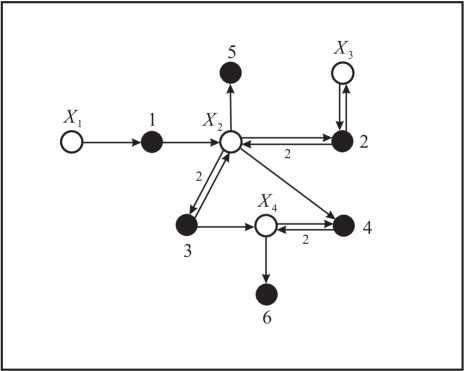
Figure 1: A directed, weighted, bipartite graphical representation of the chemical reaction system given by (2). The molecular species are represented by the white nodes, whereas, the reactions are represented by the black nodes. Edges emanating from white nodes and incident to black nodes correspond to the reactants associated with a particular reaction, whereas, edges emanating from black nodes and incident to white nodes correspond to the products of that reaction.

Although the mathematical study of the topological structure of a reaction network is an important topic of research, we will not consider this problem here. Moreover, we will not consider situations in which the topology of the network varies with time. The reader is referred to Newman (2010) and the references therein for such topological considerations. Instead, our objective is to discuss mathematical methods and computational techniques for the modeling and analysis of the dynamic behavior of reaction networks.

II.2 Stochastic dynamics on reaction networks

In many reaction networks of interest, the underlying reactions may occur at random times. If $Z_{m}(t)$ denotes the number of times that the $m\text{-th}$ reaction occurs within the time interval $[0,t)$, then $\{Z_{m}(t),t\geq 0\}$ will be a random counting process Ross (1996). By convention, we set $Z_{m}(0)=0$ (i.e., the reaction never occurs before the initial time $t=0$). We can employ the $M\times 1$ random vector $\boldsymbol{Z}(t)$ with elements $Z_{m}(t)$, $m=1,2,\ldots,M$, to characterize the state of the system at time $t>0$. $Z_{m}(t)$ is usually referred to as the degree of advancement (DA) of the $m\text{-th}$ reaction van Kampen (2007). For this reason, we refer to the multivariate counting process $\{\boldsymbol{Z}(t),t>0\}$ as the DA process.

An alternative way to characterize a reaction network is by using the $N\times 1$ random state vector

$$\boldsymbol{X}(t):=\boldsymbol{x}_{0}+\mathbb{S}\boldsymbol{Z}(t),$$ (3)

for $t\geq 0$, where $\mathbb{S}:=\mathbb{V}^{\prime}-\mathbb{V}$ is the net stoichiometric matrix of the reaction network and $\boldsymbol{x}_{0}$ is some known value of $\boldsymbol{X}(t)$ at time $t=0$. Usually, the $n\text{-th}$ element $X_{n}(t)$ of $\boldsymbol{X}(t)$ represents the population number of the $n\text{-th}$ species present in the system at time $t$, although this may not be true in certain problems (see the examples discussed in Sections III-D and III-E). We will be referring to the multivariate stochastic process $\{\boldsymbol{X}(t),t>0\}$ as the population process. For a given initial population vector $\boldsymbol{x}_{0}$, Eq. (3) allows us to uniquely determine the random population vector $\boldsymbol{X}(t)$ from the DAs $\boldsymbol{Z}(t)$, provided than $\boldsymbol{Z}(t)$ is finite with probability one.

II.2.1 Markovian dynamics

A large class of reaction networks can be characterized by Markovian dynamics, in which case we refer to them as Markovian reaction networks. Markovian reaction networks are based on the fundamental premise that, for a sufficiently small $dt$, the probability of one reaction to occur within the time interval $[t,t+dt)$ is proportional to $dt$, with proportionality factor that depends only on the species population present in the system at time $t$. Specifically, we have that $\Pr{\bigl{[}}\mbox{one reaction}~{}m~{}\mbox{occurs within}~{}[t,t+dt)\mid\boldsymbol{X}(t)=\boldsymbol{x}{\bigr{]}}$ $=$ $\pi_{m}(\boldsymbol{x})dt+o(dt)$, for some function $\pi_{m}(\boldsymbol{x})$ of the population, known as the propensity function Gillespie (2000), where $o(dt)$ is a term that goes to zero faster than $dt$. Under these assumptions, $\{Z_{m}(t),t>0\}$ is a Markovian counting process with intensity $\pi_{m}(\boldsymbol{X}(t))$. In particular, the probability $p_{\scriptscriptstyle\boldsymbol{Z}}(\boldsymbol{z};t):=\Pr[\boldsymbol{Z}(t)=\boldsymbol{z}\mid\boldsymbol{Z}(0)={\bf 0}]$ associated with this process satisfies the following partial differential equation Haseltine and Rawlings (2002); Goutsias (2005, 2006):

$$\!\!\!\!\!\!\!\!\!\!\!\!\!\!\frac{\partial p_{\scriptscriptstyle\boldsymbol{Z}}(\boldsymbol{z};t)}{\partial t}$$

$$\!\!\!\!\!\!\!\!\!\!\!=\!\!\!\sum_{m\in\mathcal{M}}\!\!{\Bigl{\{}}\alpha_{m}(\boldsymbol{z}-{\bf e}_{m})p_{\scriptscriptstyle\boldsymbol{Z}}(\boldsymbol{z}-{\bf e}_{m};t)-\alpha_{m}(\boldsymbol{z})p_{\scriptscriptstyle\boldsymbol{Z}}(\boldsymbol{z};t){\Bigr{\}}},$$ (4)

for $t>0$, where

$$\alpha_{m}(\boldsymbol{z}):=\left\{\begin{array}[]{ll}\pi_{m}(\boldsymbol{x}_{0}+\mathbb{S}\boldsymbol{z}),&\mbox{if~{}~{}$\boldsymbol{z}\geq 0$}\\[6.0pt] 0,&\mbox{otherwise}\>,\end{array}\right.$$

and ${\bf e}_{m}$ is the $m\text{-th}$ column of the $M\times M$ identity matrix. This equation is initialized by setting $p_{\scriptscriptstyle\boldsymbol{Z}}(\boldsymbol{z};0)=\Delta(\boldsymbol{z})$, where $\Delta(\boldsymbol{z})$ is the Kronecker delta function. It turns out that the population process $\{\boldsymbol{X}(t),t>0\}$ is a Markov process as well with probability $p_{\scriptscriptstyle\boldsymbol{X}}(\boldsymbol{x};t):=\Pr[\boldsymbol{X}(t)=\boldsymbol{x}\mid\boldsymbol{X}(0)=\boldsymbol{x}_{0}]$ that satisfies the following partial differential equation Gillespie (1992):

$$\!\!\!\!\!\!\!\!\!\!\!\!\!\!\frac{\partial p_{\scriptscriptstyle\boldsymbol{X}}(\boldsymbol{x};t)}{\partial t}$$

$$\!\!\!\!\!\!\!\!\!\!\!=\!\!\!\sum_{m\in\mathcal{M}}\!\!{\Bigl{\{}}\pi_{m}(\boldsymbol{x}-{\bf s}_{m})p_{\scriptscriptstyle\boldsymbol{X}}(\boldsymbol{x}-{\bf s}_{m};t)-\pi_{m}(\boldsymbol{x})p_{\scriptscriptstyle\boldsymbol{X}}(\boldsymbol{x};t){\Bigr{\}}},$$ (5)

for $t>0$, initialized by $p_{\scriptscriptstyle\boldsymbol{X}}(\boldsymbol{x};0)=\Delta(\boldsymbol{x}-\boldsymbol{x}_{0})$, where $\boldsymbol{s}_{m}$ is the $m\text{-th}$ column of the net stoichiometric matrix $\mathbb{S}$. For notational simplicity, we hide the dependency of $p_{\scriptscriptstyle\boldsymbol{X}}(\boldsymbol{x};t)$ on $\boldsymbol{x}_{0}$. Most often, Eqs. (4) and (5) are referred to as master equations although they are both special cases of the well-known forward Kolmogorov equations in the theory of Markov processes van Kampen (2007).

The previous master equations provide a suggestive interpretation on how the probabilities $p_{\scriptscriptstyle\boldsymbol{Z}}(\boldsymbol{z};t)$ and $p_{\scriptscriptstyle\boldsymbol{X}}(\boldsymbol{x};t)$ evolve as a function of time. For example, Eq. (5) implies that the probability $p_{\scriptscriptstyle\boldsymbol{X}}(\boldsymbol{x};t)$ of the population process $\boldsymbol{X}(t)$ taking value $\boldsymbol{x}$ increases during the time interval $[t,t+dt)$ by an amount $dt\sum_{m\in\mathcal{M}}\pi_{m}(\boldsymbol{x}-{\bf s}_{m})p_{\scriptscriptstyle\boldsymbol{X}}(\boldsymbol{x}-{\bf s}_{m};t)$ due to possible transitions from states $\boldsymbol{x}-\boldsymbol{s}_{m}$, $m\in\mathcal{M}$, at time $t$, to state $\boldsymbol{x}$ at time $t+dt$. However, during the same time period the probability $p_{\scriptscriptstyle\boldsymbol{X}}(\boldsymbol{x};t)$ also decreases by an amount $dt\sum_{m\in\mathcal{M}}\pi_{m}(\boldsymbol{x})p_{\scriptscriptstyle\boldsymbol{X}}(\boldsymbol{x};t)$ due to possible transitions from state $\boldsymbol{x}$ at time $t$ to states $\boldsymbol{x}+\boldsymbol{s}_{m}$, $m\in\mathcal{M}$, at time $t+dt$. Note finally that, in most practical situations, the elements of $\boldsymbol{x}$ are limited to being not larger than some finite value. As a consequence, we assume that $p_{\scriptscriptstyle\boldsymbol{X}}(\boldsymbol{x};t)=\pi_{m}(\boldsymbol{x})=0$, when at least one element of $\boldsymbol{x}$ is greater than that value.

II.2.2 Hidden Markov models

Although the DA process uniquely determines the population process via Eq. (3), the opposite is not true in general. This is due to the fact that the matrix $\mathbb{S}^{T}\mathbb{S}$ may not invertible. Invertibility of $\mathbb{S}^{T}\mathbb{S}$ is only possible when the nullity of $\mathbb{S}$ is zero, in which case $\boldsymbol{Z}(t)=(\mathbb{S}^{T}\mathbb{S})^{-1}\mathbb{S}^{T}[\boldsymbol{X}(t)-\boldsymbol{x}_{0}]$ and the DA process can be uniquely determined from the population process. Therefore, we can consider the DA process to be more informative in general than the population process. Note that, if the solution $p_{\scriptscriptstyle\boldsymbol{Z}}(\boldsymbol{z};t)$ of the master equation (4) is known, then we can calculate the probability mass function $p_{\scriptscriptstyle\boldsymbol{X}}(\boldsymbol{x};t)$ without having to solve Eq. (5). Since we are dealing with discrete random variables, we have that

$$p_{\scriptscriptstyle\boldsymbol{X}}(\boldsymbol{x};t)\>=\!\!\sum_{\boldsymbol{z}\in\mathcal{B}(\boldsymbol{x})}\!\!p_{\scriptscriptstyle\boldsymbol{Z}}(\boldsymbol{z};t),$$ (6)

for $t\geq 0$, where $\mathcal{B}(\boldsymbol{x}):=\{\boldsymbol{z}\!:~{}\boldsymbol{x}=\boldsymbol{x}_{0}+\mathbb{S}\boldsymbol{z}\}$.

In many reaction networks, it is much easier to observe the population process than the DA process, which is usually very difficult or impossible to measure. Thus, we can consider the elements of $\boldsymbol{Z}(t)$ as being the hidden state variables of the system under consideration and the elements of $\boldsymbol{X}(t)$ as being the observed state variables. If we choose to model the population process by Eq. (3), then we would be using what is known as a hidden Markov model (HMM) for our system Goutsias (2006). This opens the possibility of employing well-known techniques for the statistical analysis and stochastic control of HMMs to mathematically and computationally study stochastic dynamics on reaction networks.

II.2.3 Topological structure and propensity functions

At a first glance, Eqs. (4) and (5) may give the impression that the probability distributions $p_{\scriptscriptstyle\boldsymbol{Z}}(\boldsymbol{z};t)$ and $p_{\scriptscriptstyle\boldsymbol{X}}(\boldsymbol{x};t)$ of the DA and population processes associated with a reaction network do not depend on a detailed knowledge of the topological structure of the network. This is due to the fact that the previous master equations seem to depend only on the difference $\mathbb{S}=\mathbb{V}^{\prime}-\mathbb{V}$ between the stoichiometric matrices $\mathbb{V}$ and $\mathbb{V}^{\prime}$ and not on the individual matrices. This however is not true. It turns out that, for all reaction networks encountered in practice, the propensity function $\pi_{m}(\boldsymbol{x})$ associated with the $m\text{-th}$ reaction node in the network does not depend on all elements of the state vector $\boldsymbol{x}$ but only on those elements associated with the adjacent reactant nodes, as specified by the stoichiometric matrix $\mathbb{V}$. In other words, the propensity function does not depend on terms involving variables on non-adjacent nodes. As a consequence, the topological structure of a reaction network directly affects its dynamics through this mathematical property of the propensity functions.

III Examples

We now provide a few examples which clearly demonstrate that the previously discussed general framework for reaction networks, based on (1), is sufficiently general to characterize Markovian dynamics on many other important networks. Each example is associated with a set of “species” that affect each other’s population by interacting through well-defined “reactions.” To determine the DA and population dynamics, we only need to specify the mathematical form of the underlying propensity functions – from these, the dynamics follow by solving Eq. (4) or Eq. (5) for $p_{\scriptscriptstyle\boldsymbol{Z}}(\boldsymbol{z};t)$ and $p_{\scriptscriptstyle\boldsymbol{X}}(\boldsymbol{x};t)$, respectively.

III.1 Biochemical networks

When dealing with biochemical reactions, we usually assume that the system is well-stirred and in thermal equilibrium at fixed volume. It can be shown in this case that the probability of a randomly selected combination of reactant molecules at time $t$ to react through the $m\text{-th}$ reaction during the infinitesimally small time interval $[t,t+dt)$ is proportional to $dt$, with a proportionality factor $\kappa_{m}$ known as the specific probability rate constant of the reaction Gillespie (1992). As a consequence, $\Pr{\bigl{[}}\mbox{one reaction}~{}m~{}\mbox{occurs within}~{}[t,t+dt)\mid\boldsymbol{X}(t)=\boldsymbol{x}{\bigr{]}}$ $=$ $\kappa_{m}\gamma_{m}(\boldsymbol{x})dt+o(dt)$, where $\gamma_{m}(\boldsymbol{x})$ is the number of distinct subsets of molecules that can form a reaction complex at time $t$, given by

$$\gamma_{m}(\boldsymbol{x}) \!\!=\!\!\! \prod_{n\in\mathcal{N}}\binom{x_{n}}{\nu_{nm}}$$

$$\!\!=\!\!\! \prod_{n\in\mathcal{N}}\left[x_{n}\geq\nu_{nm}\right]\frac{x_{n}!}{\nu_{nm}!(x_{n}-\nu_{nm})!}~{},\vspace{-3pt}$$

with $[a_{1}\geq a_{2}]$ being the Iverson bracket. Note that the Iverson bracket guarantees that a reaction will proceed only if all reactants are present in the system. Moreover, we use the convention $0!=1$, so $\binom{x_{n}}{0}=1$, indicating that the rate of a reaction is only determined by the state of the reactants. As a consequence, we obtain the following propensity functions:

$$\pi_{m}(\boldsymbol{x})=\kappa_{m}\!\!\prod_{n\in\mathcal{N}}\binom{x_{n}}{\nu_{nm}}~{},\quad\mbox{for}~{}~{}m\in\mathcal{M},$$

which are said to follow the mass-action law.

We should note here that certain reactions cannot be adequately characterized by propensity functions that follow the mass-action law. For example, let us consider a reaction $X_{1}+X_{2}\rightarrow X_{3}$ that can occur only when a molecule $X_{1}$ is bound by at least one molecule $X_{2}$ at two independent binding sites with the same affinity $\theta$. It can be shown [e.g., see Dill and Bromberg (2011)] that the fraction of molecules $X_{1}$ bound by $X_{2}$ is given by $\theta x_{1}/(1+\theta x_{1})$. This leads to the following hyperbolic propensity function for the reaction:

$$\pi(x_{1},x_{2})=\frac{\kappa\theta x_{1}x_{2}}{1+\theta x_{1}},$$

where $\kappa$ is the associated specific probability rate constant. Clearly, the mathematical form of the propensity function of a given reaction depends on the underlying molecular mechanism.

III.2 Pharmacokinetic networks

Physiological pharmacokinetic models are used extensively to study the absorption, distribution, metabolism, and elimination of chemicals and drugs by the body of animals and humans. As a consequence, they are of crucial importance for drug dosing in clinical pharmacology Hardman and Limbird (2001). A large class of pharmacokinetic models is based on the notion of compartmentalization Macheras and Iliadis (2006). These models assume the existence of a central compartment (e.g., heart, lungs, brain, etc.), which serves as a site for drug administration to peripheral compartments (e.g., fat, muscles, central nervous system, and liver).

To illustrate the connection between pharmacokinetic models and Markovian reaction networks, we consider here a model for studying the effect of tetrachloroethylene, a widely used solvent, on carcinogenesis Bois et al. (1990). This model assumes a division of the human body into the lungs, which serve as the central compartment, and four peripheral compartments, namely fat tissue, poorly perfused tissue (muscles and skin), richly perfused tissue (central nervous system and viscera, except liver), and liver. To model this system, we denote by $X_{n}$ the solvent present in the $n\text{-th}$ compartment. Then, we can represent the system by $N=5$ species interacting by the following $M=10$ reactions:

$$\begin{array}[]{lrcl}\text{reaction}~{}1:{}{}&\emptyset&\rightarrow&X_{1}\\[2.0pt] \text{reaction}~{}2:{}{}&X_{1}&\rightarrow&X_{2}\\[2.0pt] \text{reaction}~{}3:{}{}&X_{2}&\rightarrow&X_{1}\\[2.0pt] \text{reaction}~{}4:{}{}&X_{1}&\rightarrow&X_{3}\\[2.0pt] \text{reaction}~{}5:{}{}&X_{3}&\rightarrow&X_{1}\\[2.0pt] \text{reaction}~{}6:{}{}&X_{1}&\rightarrow&X_{4}\\[2.0pt] \text{reaction}~{}7:{}{}&X_{4}&\rightarrow&X_{1}\\[2.0pt] \text{reaction}~{}8:{}{}&X_{1}&\rightarrow&X_{5}\\[2.0pt] \text{reaction}~{}9:{}{}&X_{5}&\rightarrow&X_{1}\\[2.0pt] \text{reaction}~{}10:{}{}&X_{5}&\rightarrow&\emptyset~{}.\\[2.0pt] \end{array}$$

The underlying reactions model the injection of solvent into lung blood (reaction 1), the exchange of one molecule of solvent between the lung blood and fat tissue (reactions 2 & 3), poorly perfused tissue (reactions 4 & 5), richly perfused tissue (reactions 6 & 7), and liver tissue (reactions 8 & 9), as well as the metabolic clearance of the solvent by the liver (reaction 10).

If we assume that all compartments are homogeneous, that the injection of solvent into the lung blood takes place at a constant rate $\kappa_{1}$, and that the probability of a randomly selected solvent molecule to move from compartment $n$ to compartment $n^{\prime}$ within an infinitesimally small time interval $[t,t+dt)$ is proportional to $dt$ with proportionality constant $\kappa_{nn^{\prime}}$, then we can model the previous pharmacokinetic system as a Markovian reaction network with linear mass-action propensity functions

$$\begin{array}[]{lll}\pi_{1}(\boldsymbol{x})=\kappa_{1},&\pi_{2}(\boldsymbol{x})=\kappa_{12}x_{1},&\pi_{3}(\boldsymbol{x})=\kappa_{21}x_{2},\\[4.0pt] \pi_{4}(\boldsymbol{x})=\kappa_{13}x_{1},&\pi_{5}(\boldsymbol{x})=\kappa_{31}x_{3},&\pi_{6}(\boldsymbol{x})=\kappa_{14}x_{1},\\[4.0pt] \pi_{7}(\boldsymbol{x})=\kappa_{41}x_{4},&\pi_{8}(\boldsymbol{x})=\kappa_{15}x_{1},&\pi_{9}(\boldsymbol{x})=\kappa_{51}x_{5},\end{array}$$

where the $n\text{-th}$ element $x_{n}$ of vector $\boldsymbol{x}$ denotes the population of tetrachloroethylene in the $n\text{-th}$ compartment. Moreover, if we assume that tetrachloroethylene metabolism in the liver is saturable according to the Michaelis-Menten relationship of enzyme kinetics Bois et al. (1990), then the propensity function of the last reaction will be given by the following nonlinear (hyperbolic) expression Sanft et al. (2011):

$$\pi_{10}(\boldsymbol{x})=\frac{Vx_{5}}{K+x_{5}},$$

where $V,K$ are two parameters associated with the underlying metabolic mechanism.

III.3 Epidemiological networks

Epidemiological networks study the spread of infectious diseases or agents through a population of individuals. Although numerous publications can be found on the subject, we refer the reader to Newman (2010) for an elementary introduction to epidemiological networks. For a mathematical review of deterministic epidemiological models, see Hethcote (2000), whereas, for a stochastic modeling approach to epidemiological modeling, see Chen and Bokka (2005).

To illustrate the connection between epidemiological networks and Markovian reaction networks, we consider the simplest and most widely used model, known as the SIR epidemic model. In this model, an individual in a population can be in one of three states with respect to a disease: susceptible (S), infected (I), or resistant (R). According to this model, there are two types of interactions that an individual may undergo: (a) if a susceptible individual comes into contact with an infectious individual, the susceptible person can be infected, and (b) an infected individual may become resistant if his immune system fights off the infection and confers resistance, or if the individual dies by the infection. These interactions can be modeled by a reaction network comprised of $N=3$ species (S, I, and R) that interact through the following $M=2$ reactions:

$$\begin{array}[]{rcl}X_{1}+X_{2}&\rightarrow&2X_{2}\\[2.0pt] X_{2}&\rightarrow&X_{3}~{},\end{array}$$ (7)

where $X_{1}=\text{S}$, $X_{2}=\text{I}$ and $X_{3}=\text{R}$. In this case,

$$\mathbb{V}=\left[\begin{array}[]{cc}1&0\\ 1&1\\ 0&0\end{array}\right]\!\!,~{}\mathbb{V}^{\prime}=\left[\begin{array}[]{cc}0&0\\ 2&0\\ 0&1\end{array}\right]\!\!,~{}\mbox{and}~{}\mathbb{S}=\left[\begin{array}[]{rr}-1&0\\ 1&-1\\ 0&1\end{array}\right]\!.$$

We can now assume that the probability of a randomly selected susceptible individual at time $t$ to become infected by a randomly selected infectious individual during an infinitesimally small time interval $[t,t+dt)$ is proportional to $dt$, with proportionality factor $\kappa_{1}$ that does not depend on the particular individuals involved. Moreover, we can assume that the probability of a randomly selected infected individual at time $t$ to recover or die from the disease during $[t,t+dt)$ is also proportional to $dt$, with proportionality factor $\kappa_{2}$ that does not depend on the particular infected individual. Then, the previous interactions lead to a Markovian reaction network with mass-action propensity functions given by Chen and Bokka (2005)

$$\pi_{1}(x_{1},x_{2},x_{3})=\kappa_{1}x_{1}x_{2}\quad\mbox{and}\quad\pi_{2}(x_{1},x_{2},x_{3})=\kappa_{2}x_{2},$$

where $x_{1},x_{2},x_{3}$ are the populations of susceptible, infectious, and resistant individuals, respectively.

We can use the previous 3-species/2-reactions motif, given by (7), to construct more complex Markovian reaction networks that model the spread of an infectious disease in a population of individuals grouped into classes (e.g., households, work spaces, cities, etc.); see Ben-Zion et al. (2010). We may group, for example, individuals into two classes, those living in Baltimore and Philadelphia, and give each class its own distinct set of variables, namely $X_{1},X_{2},X_{3}$, for susceptible, infected, and resistant individuals in Baltimore, as well as $X_{4},X_{5},X_{6}$, for susceptible, infected, and resistant individuals in Philadelphia. Each class will be characterized by the previous 3-species/2-reactions motif, resulting in the following four reactions:

$$\begin{array}[]{rcl}X_{1}+X_{2}&\rightarrow&2X_{2}\\[2.0pt] X_{2}&\rightarrow&X_{3}\\[2.0pt] X_{4}+X_{5}&\rightarrow&2X_{5}\\[2.0pt] X_{5}&\rightarrow&X_{6}~{}.\end{array}$$

In this case however there is also a flow (by air, road, or rail) of individuals between the two different cities, which we can model by using the following six reactions:

$$\begin{array}[]{rcl}X_{1}&\rightarrow&X_{4}\\[2.0pt] X_{4}&\rightarrow&X_{1}\\[2.0pt] X_{2}&\rightarrow&X_{5}\\[2.0pt] X_{5}&\rightarrow&X_{2}\\[2.0pt] X_{3}&\rightarrow&X_{6}\\[2.0pt] X_{6}&\rightarrow&X_{3}\>.\end{array}$$

The propensity functions associated with these new reactions will be proportional to the population of the input species, with the proportionality factor being the specific probability rate constant of an individual traveling from one city to the other. In this fashion, we can build complex Markovian reaction network models for epidemiological dynamics that are more realistic and more predictive than traditional deterministic models.

Likewise, new reactions may be incorporated into the epidemiological network to account for additional transitions between states. For instance, if we assume that a vaccine is available, then we must include the reaction $X_{1}\rightarrow X_{3}$ in the formulation. Vital dynamics (i.e., births and deaths) may also be included in this fashion. For example, if infants born at a fixed rate are always susceptible, then the reaction $\emptyset\rightarrow X_{1}$ must be included in the system. Finally, one may consider social networks on which epidemiological networks reside. Specifically, age stratification in the population Hethcote (2000), or the scale-free structure of social/sexual networks Newman (2010), may be handled in a manner similar – albeit not identical – to the aforementioned geographic considerations.

III.4 Ecological networks

Ecological networks aim to study interactions among organisms living in a particular area as well as between these organisms and nonliving physical components of the environment, such as air, soil, water, and sunlight. The main objective of this type of network is to model how mass and energy are transferred from primary producers (or autotrophs), who generate their own energy from the sun’s rays, up to the apex predators who gather their energy and body mass through the consumption of prey lower in the food chain. We illustrate here the fact that ecological networks can also be modeled as Markovian reaction networks using a simple example.

Consider a food web comprised of grass ($X_{1}$), rabbits ($X_{2}$) and wolves ($X_{3}$), whose net mass at time $t$ is given by $X_{1}(t)$, $X_{2}(t)$ and $X_{3}(t)$, respectively. These states can take non-integer values. In particular, $X_{1}(t)=x$ means that, at time $t$, the mass of grass equals $x$-times some reference value, and likewise for rabbits and wolves. More advanced models may also choose to keep track of the number of individuals Datta et al. (2010). Here however we consider a common situation in which the net mass of each species is sufficient to describe the system.

We can assume that changes in mass distribution are caused by discrete steps in body size as predators eat prey as well as by the mortality that comes with this process. In particular, we can model the predation of grass by rabbits and rabbits by wolves with the following two reactions Dilão and Domingos (2000):

$$\begin{array}[]{rcl}X_{1}+X_{2}&\rightarrow&(1+a_{1})X_{2}\\[6.0pt] X_{2}+X_{3}&\rightarrow&(1+a_{2})X_{3}\>,\end{array}$$

where $a_{1},a_{2}>0$ are constants representing the conversion factor of mass. Moreover, when rabbits or wolves die for reasons other than predation they fertilize the grass. We can model this conversion by Dilão and Domingos (2000)

$$\begin{array}[]{rcl}X_{2}&\rightarrow&b_{1}X_{1}\\[6.0pt] X_{3}&\rightarrow&b_{2}X_{1}\>,\end{array}$$

where $b_{1},b_{2}>0$ are appropriately chosen recycling constants. As a consequence, the stoichiometric matrices of the resulting reaction network, comprised of the $N=3$ species and the $M=4$ reactions above, are given by

$$\mathbb{V}=\left[\begin{array}[]{cccc}1&0&0&0\\ 1&1&1&0\\ 0&1&0&1\end{array}\right]\!\!,\quad\mathbb{V}^{\prime}=\left[\begin{array}[]{cccc}0&0&b_{1}&~{}~{}b_{2}\\ 1+a_{1}&0&0&~{}~{}0\\ 0&1+a_{2}&0&~{}~{}0\end{array}\right]\!\!,$$

$$\mathbb{S}=\left[\begin{array}[]{rrrr}-1&0&b_{1}&b_{2}\\ a_{1}&-1&-1&0\\ 0&a_{2}&0&-1\end{array}\right]\!\!.$$

Under appropriate assumptions, similar to the ones made before, the previous interactions lead to a Markovian reaction network with mass-action propensity functions given by Dilão and Domingos (2000)

$$\begin{array}[]{ll}\pi_{1}(\boldsymbol{x})=\kappa_{1}[x_{1},x_{2}\geq 1]x_{1}x_{2},&\!\!\!\!\!\!\!\!\!\!\!\!\pi_{2}(\boldsymbol{x})=\kappa_{2}[x_{2},x_{3}\geq 1]x_{2}x_{3}\\[6.0pt] \pi_{3}(\boldsymbol{x})=\kappa_{3}[x_{2}\geq 1]x_{2},&\!\!\!\!\!\!\!\!\!\!\!\!\pi_{4}(\boldsymbol{x})=\kappa_{4}[x_{3}\geq 1]x_{3},\end{array}$$

where the Iverson brackets are used to make sure that the reactions occur only when the net mass of a reactant species is at least as large as the corresponding reference value. Here, $\kappa_{1}$ is the specific probability rate constant of rabbits eating grass, $\kappa_{2}$ is the specific probability rate constant of wolves eating rabbits, and $\kappa_{3},\kappa_{4}$ are the specific probability rate constant of natural deaths of rabbits and wolves, respectively.

More complicated ecological reaction network models can include geographic considerations, direct competition, mutualism, and more complex food chains Lässig et al. (2001); Powell and Boland (2009); Thébault and Fontaine (2010). In addition, epidemiological networks can be combined with ecological networks to study the effects of a disease on a given ecosystem Auger et al. (2009).

III.5 Social networks

Recently, interest has emerged in developing mathematical models for social networks that can be used to better understand human behavior. In particular, much effort has been devoted to studying dynamics on social networks Moreno et al. (2004); Antal et al. (2006); Weidlich (2006); Zanette and Gil (2006); Hill et al. (2010); Masuda et al. (2010), a problem that has been investigated by the physics community many decades ago Haken (1975). Several models for dealing with dynamic processes on social networks are currently available, with many fitting nicely into the Markovian reaction framework discussed in this review. As an example, we focus on a model of opinion formation in social networks, a process that is of political, marketing, and general sociological interest.

The critical behavior of a society moving from a liberal to a totalitarian political system can be evaluated when individuals are endowed with two separate opinions: a publicly pronounced and a privately held opinion for/against the ideology of the ruling party. The public and private opinions of an individual can be different when, for example, public dissent against the ruling ideology is a punishable offence. Along these lines, let us consider a fixed homogeneous group of $2L$ individuals who react in the same manner to a given situation. An individual simultaneously holds a public and a private opinion that each takes values $1/2$ or $-1/2$ if it is for or against the ruling ideology, respectively. Let us denote by $X_{1}$ the net public opinion, which corresponds to the sum of the publicly held opinions of all $2L$ individuals. Likewise, let us denote by $X_{2}$ the net private opinion. We are now dealing with $N=2$ species interacting through the following $M=4$ reactions:

$$\begin{array}[]{ll}\text{reaction}~{}1:~{}~{}X_{1}+X_{2}\rightarrow 2X_{1}+X_{2}\\[4.0pt] \text{reaction}~{}2:~{}~{}X_{1}+X_{2}\rightarrow X_{2}\\[4.0pt] \text{reaction}~{}3:~{}~{}X_{1}+X_{2}\rightarrow X_{1}+2X_{2}\\[4.0pt] \text{reaction}~{}4:~{}~{}X_{1}+X_{2}\rightarrow X_{1}.\end{array}$$ (8)

The first two reactions model the influence of net private opinion $X_{2}$ on the net public opinion $X_{1}$ that results in a single individual changing her public opinion in support of (reaction 1) or against (reaction 2) the ruling ideology. In this case, the net private opinion remains unchanged, whereas, the net public opinion is increased by one in reaction 1 [due to a value change from $-1/2$ (against) to $1/2$ (for)] and decreased by one in reaction 2 [due to a value change from $1/2$ (for) to $-1/2$ (against)]. Likewise, the subsequent two reactions model the influence of net public opinion $X_{1}$ on the net private opinion $X_{2}$ that results in a single individual changing her private opinion in support of (reaction 3) or against (reaction 4) the ruling ideology. These reactions are governed by the following propensity functions Weidlich (2006):

$$\begin{array}[]{l}\pi_{1}(\boldsymbol{x})=\kappa_{1}(L-x_{1})\exp(a_{1}x_{1}+a_{2}x_{2})\\[4.0pt] \pi_{2}(\boldsymbol{x})=\kappa_{1}(L+x_{1})\exp(-a_{1}x_{1}-a_{2}x_{2})\\[4.0pt] \pi_{3}(\boldsymbol{x})=\kappa_{2}(L-x_{2})\exp(a_{3}x_{1})\\[4.0pt] \pi_{4}(\boldsymbol{x})=\kappa_{2}(L+x_{2})\exp(-a_{3}x_{1}),\end{array}$$ (9)

where $x_{1}$, $x_{2}$ represent the net values of all publicly and privately held opinions, respectively, $\kappa_{1},\kappa_{2}>0$ are two specific probability rate constants associated with the four reactions, and $a_{1}\geq 0$, $a_{2}>0$, $a_{3}$ are three model parameters. Note that $x_{1}$ and $x_{2}$ are integer-valued with $-L\leq x_{1},x_{2}\leq L$, where $-L$ represents total disapproval and $L$ represents total approval of the ruling ideology.

Parameter $a_{1}\geq 0$ controls pressure inflicted on public opinion due, for example, to oppression of this opinion by the ruling party (the value of this parameter is zero in the U.S. where free speech is protected, but strictly positive in countries where public dissidence has consequences). On the other hand, parameter $a_{2}>0$ controls the influence of privately held beliefs on publicly stated opinions, whereas, parameter $a_{3}$ controls how affirmative (for $a_{3}>0$) or dissident (for $a_{3}<0$) the private opinion is towards the ruling ideology. When the values of $a_{1}$ and $a_{3}$ vary, an abrupt change from a liberal to a totalitarian political system can be observed Weidlich (2006). This critical social behavior predicted by the model is reminiscent to the well-known phenomenon of phase transition in statistical mechanics and provides a crucial focus of study when dealing with opinion spreading in social networks.

III.6 Neural networks

A discussion on reaction networks cannot be complete without mentioning biological neural networks. With 100 billion or more neurons in the human brain connected by 100-500 trillion synapses, there is no other reaction network that can compete in size and complexity.

There is a large body of literature surrounding the modeling and analysis of biological neural networks. As an example, we consider a Markovian reaction model for neural networks recently proposed by Benayoun et al. (2010) that is intuitive enough for novices in neurobiology to comprehend and yet rich enough to be a viable candidate for understanding many features of this preeminent reaction network. The model consists of $L$ neurons, with each neuron being in either a quiescent or an active state. Let $X_{2l-1}$ and $X_{2l}$ denote a quiescent or active neuron $l$, respectively. We can assign the following two reactions to the $l\text{-th}$ neuron in the network:

$$\begin{array}[]{rcl}X_{2l-1}+{\displaystyle\sum_{l^{\prime}\neq\>l}}~{}\nu_{l^{\prime}l}X_{2l^{\prime}}&\rightarrow&X_{2l}+{\displaystyle\sum_{l^{\prime}\neq\>l}}~{}\nu_{l^{\prime}l}X_{2l^{\prime}}\\[6.0pt] X_{2l}&\rightarrow&X_{2l-1},\end{array}$$ (10)

where $\nu_{ij}$ measures the synaptic weight between neurons $i$ and $j$, with a positive value indicating an excitatory synapsis and a negative value indicating an inhibitory synapsis. Note that the first reaction models transition of the $l\text{-th}$ neuron from the quiescent to the active state, which is assumed to be influenced by appropriately weighted active neurons $X_{2l^{\prime}}$, $l^{\prime}\not=l$, in the network [see Eq. (11) below] that act as “catalysts.” On the other hand, the second reaction models transition of the neuron from the active to the quiescent state, which is assumed to occur constitutively. As a consequence, we obtain a reaction network with $N=2L$ species and $M=2L$ reactions.

We can describe this system by a $2L\times 1$ state vector $\boldsymbol{x}$ with binary-valued $0/1$ elements $x_{2l-1}$, $x_{2l}$ indicating the state of the $l\text{-th}$ neuron (with $0$ being quiescent and $1$ being active). Due to the fact that a neuron must be either quiescent or active, the state variables must satisfy the mass conservation relationships $x_{2l-1}+x_{2l}=1$, for $l=1,2,\ldots,L$. It has been suggested by Benayoun et al. (2010) that the probability of the $l\text{-th}$ neuron becoming active during an infinitesimally small time interval $[t,t+dt)$, given that the neuron is quiescent at time $t$, can be taken to be $x_{2l-1}[\phi_{l}(\boldsymbol{x})>0]\tanh[\phi_{l}(\boldsymbol{x})]dt+o(dt)$, where $[a>0]$ is the Iverson bracket and $\phi_{l}$ is the net synaptic input to the $l\text{-th}$ neuron, given by

$$\phi_{l}(\boldsymbol{x})=\sum_{l^{\prime}\neq\>l}\nu_{l^{\prime}l}x_{2l^{\prime}}+h_{l},$$ (11)

with $h_{l}$ being an external input to the neuron. The term $x_{2l-1}$ ensures that the neuron becomes active within $[t,t+dt)$ only when it is quiescent at time $t$. As a consequence, the propensity of the first reaction in (10) will be given by

$$\pi_{2l-1}(\boldsymbol{x})=x_{2l-1}[\phi_{l}(\boldsymbol{x})>0]\tanh[\phi_{l}(\boldsymbol{x})],$$ (12)

and therefore depends on the synaptic inputs from neurons connected to the $l\text{-th}$ neuron and any external input to that neuron. On the other hand, if we assume that the $l\text{-th}$ neuron decays from an active to a quiescent state at a constant rate $\gamma_{l}$, then the propensity of the second reaction will be given by

$$\pi_{2l}(\boldsymbol{x})=\gamma_{l}x_{2l},$$ (13)

where the term $x_{2l}$ ensures that the neuron becomes inactive within $[t,t+dt)$ only when it is active at time $t$.

III.7 Multi-agent networks

The study of multi-agent networks focuses on systems in which many intelligent agents, such as autonomous vehicles that observe and act upon their environment, interact with each other to achieve a certain goal. To illustrate the fact that multi-agent systems can also be modeled as Markovian processes on reaction networks, we consider here a system comprised of $L$ autonomous unmanned vehicles (AUVs) that can move over a two-dimensional bounded rectangular space in a discrete fashion Xi et al. (2006). For simplicity, we assume that, at each step, an AUV located at a discrete point $(i,j)$ in space can move towards one of four possible directions, namely east to point $(i+1,j)$, west to point $(i-1,j)$, north to point $(i,j+1)$, or south to point $(i,j-1)$. We want to develop a mathematical approach that can be used to describe vehicular motion so that the AUVs reach a spatial configuration $\boldsymbol{x}$ at steady-state with desired probability $\rho(\boldsymbol{x})$ which assigns high probability over configurations that maximize a given design objective and low or zero probability over the remaining configurations. The construction of such probability can be thought of as an inverse problem that can be solved using a statistical mechanics approach, as the one proposed by Cohn and Kumar (2009).

In the following, we employ two species $X_{2l-1}$ and $X_{2l}$ whose populations $x_{2l-1}$ and $x_{2l}$ denote the position of the $l\text{-th}$ AUV on the two-dimensional rectangular grid. For example, if the $l\text{-th}$ vehicle is located at point $(i,j)$ on the grid, then $x_{2l-1}=i$ and $x_{2l}=j$. We can now characterize the motion of all AUVs in the multi-agent network under consideration by $N=2L$ species interacting through the following $M=4L$ reactions:

$$\!\!\!\!\!\!\!\!\!\!\!\!\!\!\!\!\!\!\!\!X_{2l-1}+X_{2l}+{\displaystyle\sum_{l^{\prime}\neq\>l}(X_{2l^{\prime}-1}+X_{2l^{\prime}})}\rightarrow$$

$$~{}~{}~{}~{}~{}~{}2X_{2l-1}+X_{2l}+{\displaystyle\sum_{l^{\prime}\neq\>l}(X_{2l^{\prime}-1}+X_{2l^{\prime}})}$$

$$\!\!\!\!\!\!\!\!\!\!\!\!\!\!\!\!\!\!\!\!X_{2l-1}+X_{2l}+{\displaystyle\sum_{l^{\prime}\neq\>l}(X_{2l^{\prime}-1}+X_{2l^{\prime}})}\rightarrow$$

$$~{}~{}~{}~{}~{}~{}X_{2l}+{\displaystyle\sum_{l^{\prime}\neq\>l}(X_{2l^{\prime}-1}+X_{2l^{\prime}})}$$

$$\!\!\!\!\!\!\!\!\!\!\!\!\!\!\!\!\!\!\!\!X_{2l-1}+X_{2l}+{\displaystyle\sum_{l^{\prime}\neq\>l}(X_{2l^{\prime}-1}+X_{2l^{\prime}})}\rightarrow$$

$$~{}~{}~{}~{}~{}~{}X_{2l-1}+2X_{2l}+{\displaystyle\sum_{l^{\prime}\neq\>l}(X_{2l^{\prime}-1}+X_{2l^{\prime}})}$$

$$\!\!\!\!\!\!\!\!\!\!\!\!\!\!\!\!\!\!\!\!X_{2l-1}+X_{2l}+{\displaystyle\sum_{l^{\prime}\neq\>l}(X_{2l^{\prime}-1}+X_{2l^{\prime}})}\rightarrow$$

$$~{}~{}~{}~{}~{}~{}X_{2l-1}+{\displaystyle\sum_{l^{\prime}\neq\>l}(X_{2l^{\prime}-1}+X_{2l^{\prime}})}\>.$$ (14)

The first two reactions model one-step motion of the $l\text{-th}$ AUV towards east/west, whereas, the other two reactions model one-step motion towards north/south. Note that, when the first reaction occurs, the horizontal position $i$ of the $l\text{-th}$ AUV is increased by one (transition from $X_{2l-1}$ to $2X_{2l-1}$), whereas its vertical position $j$ remains unchanged (transition from $X_{2l}$ to itself). Moreover, this is done by using the positions $X_{2l^{\prime}-1}$, $X_{2l^{\prime}}$, $l^{\prime}\not=l$, of the remaining vehicles [see Eq. (16) below], which act as “catalysts” of the reaction. Similar remarks apply for the other three reactions as well.

Let us now define the potential energy $V(\boldsymbol{x})$ of the reaction system being in configuration $\boldsymbol{x}$ at steady-state by

$$V(\boldsymbol{x}):=\left\{\begin{array}[]{cl}-\ln{\displaystyle\frac{\rho(\boldsymbol{x})}{\rho(\boldsymbol{x}_{0})}},&\quad\mbox{for~{}~{}$\boldsymbol{x}\in\mathcal{D}$}\\[12.0pt] \infty,&\quad\mbox{otherwise},\end{array}\right.$$ (15)

where $\mathcal{D}$ is a set that contains all permissible vehicle configurations (e.g., $\boldsymbol{x}$ should not allow two vehicles to occupy the same grid position or positions occupied by obstacles, thus avoiding collisions or assignment of vehicles to grid positions outside the bounded rectangular region). Moreover, $\boldsymbol{x}_{0}\in\mathcal{D}$ is an appropriately chosen reference configuration of zero potential energy. Given that $\boldsymbol{X}(t)=\boldsymbol{x}$, we can assume that, during the infinitesimally small time interval $[t,t+dt)$, the $l\text{-th}$ AUV can move one step towards east if two events take place: (a) during $[t,t+dt)$, the AUV initiates motion with probability that is proportional to $dt$, with proportionality factor $\kappa_{l}$, and (b) given that the AUV initiates motion during $[t,t+dt)$, it moves with probability $\exp\left\{-V(\boldsymbol{x}+\boldsymbol{s}_{4l-3})\right\}$, where $\boldsymbol{s}_{m}$ denotes the $m\text{-th}$ column of the net stoichiometric matrix of the reaction network given by (14). As a consequence, the AUV will be moving east with higher probability if the motion produces a larger reduction in potential energy. Note that parameter $\kappa_{l}$ controls the speed of the $l\text{-th}$ vehicle, with higher values of $\kappa_{l}$ resulting in faster motion.

By making similar assumptions for vehicle motion towards the other three directions, the dynamics on the reaction network given by (14) will be Markovian with propensity functions

$$\pi_{m}(\boldsymbol{x})=\kappa_{l}e^{-V(\boldsymbol{x}+\boldsymbol{s}_{m})},$$ (16)

for $m=4l-3,4l-2,4l-1,4l$, $l=1,2,\ldots,L$. Note that $\boldsymbol{s}_{4l-3}$, $\boldsymbol{s}_{4l-2}$, $\boldsymbol{s}_{4l-1}$ and $\boldsymbol{s}_{4l}$ equal ${\textbf{e}}_{2l-1}$, $-{\textbf{e}}_{2l-1}$, ${\textbf{e}}_{2l}$, and $-{\textbf{e}}_{2l}$, respectively, where ${\textbf{e}}_{m}$ is the $m\text{-th}$ column of the $2L\times 2L$ identity matrix. It turns out that the resulting master equation governing the population process $\boldsymbol{X}(t)$ has a unique stationary distribution $\overline{p}_{\scriptscriptstyle\bf X}(\boldsymbol{x}):=\lim_{t\rightarrow\infty}p_{\scriptscriptstyle\boldsymbol{X}}(\boldsymbol{x};t)$, given by the Gibbs distribution

$$\overline{p}_{\scriptscriptstyle\bf X}(\boldsymbol{x})=\frac{1}{\zeta}\>e^{-V(\boldsymbol{x})},$$ (17)

where

$$\zeta:=\sum_{\boldsymbol{x}}e^{-V(\boldsymbol{x})}$$ (18)

is the associated partition function. As a consequence of Eqs. (15), (17) and (18), we have that $\overline{p}_{\scriptscriptstyle\bf X}(\boldsymbol{x})=\rho(\boldsymbol{x})$. Therefore, the AUVs will asymptotically position themselves in the two-dimensional space at locations $\boldsymbol{x}$ with probability $\rho(\boldsymbol{x})$, as desired.

III.8 Evolutionary game theory

Game theory deals with mathematical models of conflict and cooperation among intelligent and rational individuals. Evolutionary game theory extends the paradigm of classical game theory by removing some stringent assumptions and by naturally incorporating the dynamic aspects of learning and experimentation into the problem.

As an example of how evolutionary game theory can fit within the current context, suppose that a population of $L$ individuals play with each other a game with $N$ possible strategies $X_{1},X_{2},\ldots,X_{N}$. Let $X_{n}(t)$ be the number of individuals playing strategy $X_{n}$ at time $t$. Here, we consider a simple situation in which each individual competes with all other individuals. However, the framework presented in this paper is also capable of handling more general situations, such as those discussed by Szabo and Fath (2007). Given that $\boldsymbol{X}(t)=\boldsymbol{x}$, let $P_{n}(\boldsymbol{x})$ be the payoff to an individual playing the $n\text{-th}$ strategy at time $t$. Based on the current payoff, this individual may decide at a random time to follow a new strategy $X_{n^{\prime}}$ in an attempt to improve his payoff. This can be modeled by the following $M=N(N-1)$ reactions:

$$X_{n}+X_{n^{\prime}}+\!\!\!\!\sum_{n^{\prime\prime}\not=\>n,n^{\prime}}\!\!\!\!\!X_{n^{\prime\prime}}~{}\rightarrow~{}2X_{n^{\prime}}+\!\!\!\!\sum_{n^{\prime\prime}\not=\>n,n^{\prime}}\!\!\!\!\!X_{n^{\prime\prime}},\quad n^{\prime}\neq n.$$

Note that, in this case, the number of individuals $X_{n^{\prime\prime}}$ that follow strategies other than $n$ and $n^{\prime}$ affect the transition of an individual from strategy $n$ to strategy $n^{\prime}$ [see Eq. (19) below] without changing their own strategies and, therefore, act as “catalysts.”

There are many alternative propensity functions that can be chosen to dictate when players will change their strategy, with each corresponding to different learning techniques or update rules Szabo and Fath (2007). A common choice however is given by the imitation rule of the Moran process Moran (1962):

$$\pi(\boldsymbol{x})=\kappa\>\frac{x_{n}}{L}\>\frac{x_{n^{\prime}}P_{n}(\boldsymbol{x})}{\sum_{n^{\prime\prime}\in\mathcal{N}}x_{n^{\prime\prime}}P_{n^{\prime\prime}}(\boldsymbol{x})}\>,$$ (19)

where $\kappa>0$ is a specific probability rate constant detailing how often individuals choose to update their strategies. The second term in Eq. (19) is the fraction of individuals playing strategy $X_{n}$, whereas, the third term is the fraction of the net payoff paid to individuals who play strategy $X_{n^{\prime}}$. These propensity functions have been originally developed to model natural selection and genetic drift in an asexually reproducing population of $N$ genetically distinct individuals, where each genotype represents a strategy and the payoffs provide measures of reproductive fitness.

III.9 Petri nets

Petri nets have been extensively used to describe discrete-event distributed systems, a class of systems that are of particular interest in computer science applications Diaz (2009). A Petri net is a weighted, directed, bipartite graph, in which the nodes represent places and transitions. Places model passive system components, whereas, transitions correspond to events that inter-convert places. Directed arcs join places to transitions (connect places that can be converted during a transition) and transitions to places (connect a transition with the corresponding products). Weights associated with arcs indicate the multiplicity of the arc. Each place is associated with tokens, indicating the number of existing places. Whether or not a transition takes place is described by a rule, which may be deterministic or stochastic Haas (2002); Diaz (2009), that depends on the number of tokens available in the places connecting to the transition by incoming arcs. The occurrence of a transition results in removing a token from the input places and adding a token to the output places of the transition.

The flow of tokens on a Petri net can be used to model the dynamics on a reaction network. As a matter of fact, a number of investigators (including Petri himself) have already proposed using Petri nets for modeling biochemical reaction systems Reddy et al. (1996); Goss and Peccoud (1998); Chaouiya (2007); Heiner et al. (2008). This approach however is very similar to traditional methods for modeling biochemical reaction systems based on first-order differential equations or the chemical master equation, which have been extensively studied in the literature Gillespie (1992); Heinrich and Schuster (1996). In particular, Markovian Petri nets are identical to the Markovian reaction networks considered in this review, with the places playing the role of species and the transitions representing reactions. It is however important to carefully study the theory of stochastic Petri nets Haas (2002), since many results derived in that theory will likely prove very useful for the analysis of the Markovian reaction networks reviewed in this paper.

IV Solving the master equation

Although the algebraic form of the master equations (4) and (5) is simple, solving these equations [i.e., calculating the probabilities $p_{\scriptscriptstyle\boldsymbol{Z}}(\boldsymbol{z};t)$ and $p_{\scriptscriptstyle\boldsymbol{X}}(\boldsymbol{x};t)$ at each time $t>0$] is a very difficult task in general. Many methods have been proposed in the literature to address this problem, which can be grouped into the six general categories depicted in Fig. 2. In the following, we discuss the most prominent techniques available to date. Whether a technique can be applied to a particular problem depends on the size and complexity of the reaction network at hand.

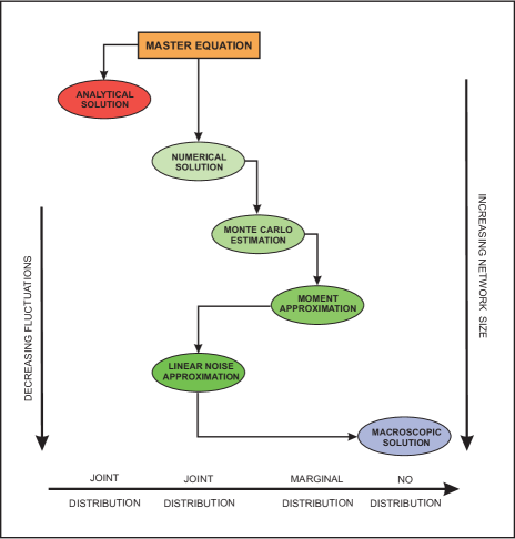
Figure 2: Six methods for solving the master equation. Some methods can be used to approximate the joint probability distributions of the DA and population processes while other methods can only be used to approximate marginal distributions. Analytical solutions can be obtained only in special cases. Numerical solutions are currently limited to small reaction networks. Large networks require use of a moment approximation scheme or adoption of linear noise approximation method as opposed to Monte Carlo sampling. For large reaction networks, computing the macroscopic solution may be the only feasible choice. This solution however can only be trusted at low fluctuation levels.

IV.1 Exact analytical solution

Deriving exact analytical solutions for $p_{\scriptscriptstyle\boldsymbol{Z}}(\boldsymbol{z};t)$ and $p_{\scriptscriptstyle\boldsymbol{X}}(\boldsymbol{x};t)$ is possible only in simple cases [e.g., see McQuarrie (1963); McQuarrie et al. (1964); Darvey and Staff (1966); Leonard and Reichl (1990); Laurenzi (2000); Gadgil et al. (2005); Zhang et al. (2005); Heuett and Qian (2006); Jahnke and Huisinga (2007); Gardiner (2010)]. For example, an analytical solution for the master equation (5) can be derived in the case of a linear reaction network (i.e., a network with linear propensity functions). It has been shown by Gadgil et al. (2005) that, for closed linear reaction networks (i.e., linear reaction networks with fixed net population), the solution of the master equation (5) is a multinomial distribution, provided that the initial joint distribution is also multinomial. Moreover, for open linear reaction networks (i.e., linear reaction networks with varying net population), the solution of the master equation (5) is a product Poisson distribution, provided that the initial joint distribution is also product Poisson [see also Heuett and Qian (2006)]. These results are special cases of a more general result derived by Jahnke and Huisinga (2007) who have shown that the probability distribution $p_{\scriptscriptstyle\boldsymbol{X}}(\boldsymbol{x};t)$ of the population process in a linear reaction network with initial state $\boldsymbol{x}_{0}$ can be expressed as the convolution of multinomial and product Poisson distributions with time-dependent parameters that evolve according to well-defined systems of first-order linear differential equations [see also Zhang et al. (2005)].

IV.2 Numerical solution

A substantial research effort has recently been focused on approximately solving the master equation (5) using numerical techniques. Although the methods developed so far show promise for addressing this problem, they are mostly limited to relatively small reaction networks. For this reason, we only provide a brief discussion here. The interested reader can find details in the references.

The master equation (5) can be expressed as a linear system of coupled first-order differential equations, given by

$$\frac{d\boldsymbol{p}(t)}{dt}=\mathbb{P}\>\boldsymbol{p}(t),$$ (20)

for $t>0$, where $\boldsymbol{p}(t)$ is a $K\times 1$ vector that contains the nonzero probabilities $p_{\scriptscriptstyle\boldsymbol{X}}(\boldsymbol{x};t)$, $\boldsymbol{x}\in\mathcal{X}$, of the population process $\boldsymbol{X}(t)$ and $\mathbb{P}$ is a large $K\times K$ sparse matrix whose structure can be inferred directly from the master equation. For example, when the columns of the stoichiometric matrix $\mathbb{S}$ are all different from each other, the only nonzero elements of the $i\text{-th}$ column of $\mathbb{P}$ are the $M$ off-diagonal elements, whose values are given by $\pi_{m}(\boldsymbol{x}_{i})$, and the diagonal element, whose value is given by $-\sum_{m=1}^{M}\pi_{m}(\boldsymbol{x}_{i})$, where $M\ll K$ is the number of reactions. If we assume that the cardinality $K$ of the state-space $\mathcal{X}$ is finite, then we can calculate the probabilities $p_{\scriptscriptstyle\boldsymbol{X}}(\boldsymbol{x};t)$ by solving Eq. (20), in which case

$$\boldsymbol{p}(t)=\exp(t\mathbb{P})\>\boldsymbol{p}(0),$$ (21)

for $t>0$. This simple idea has led to a numerical technique, proposed by Munsky and Khammash (2006), for approximately solving the master equation known as finite state projection (FSP). This method requires an appropriate truncation of the state-space to determine the smallest possible set $\mathcal{X}$ and development of a computationally feasible algorithm for calculating the matrix exponential in Eq. (21).

Although a number of methods are available for computing matrix exponentials [e.g., see Moler and van Loan (2003)], we briefly discuss here a popular technique known as Krylov subspace approximation (KSA) method Sidje (1998); Sidje and Stewart (1999). For a sufficiently small time step $\tau>0$, this is the best available method for approximating the vector $\boldsymbol{p}(t+\tau)=\exp(\tau\mathbb{P})\>\boldsymbol{p}(t)$, when $\mathbb{P}$ is a large and sparse matrix. This is done by using a polynomial series expansion of the form:

$$\widehat{\boldsymbol{p}}(t+\tau)=c_{0}\boldsymbol{p}(t)+c_{1}\tau\mathbb{P}\boldsymbol{p}(t)+\cdots+c_{\scriptscriptstyle K_{0}-1}(\tau\mathbb{P})^{K_{0}-1}\boldsymbol{p}(t),$$

where the coefficients $c_{0},c_{1},\ldots,c_{\scriptscriptstyle K_{0}-1}$ are estimated by minimizing the least-squares error $||\boldsymbol{p}(t+\tau)-\widehat{\boldsymbol{p}}(t+\tau)||_{2}^{2}$. It turns out that the optimal $K_{0}$-th order polynomial approximation of $\boldsymbol{p}(t+\tau)$ is a point in the $K_{0}$-dimensional Krylov subspace $\mathcal{K}(t)=\text{span}\!\left\{\boldsymbol{p}(t),\tau\mathbb{P}\boldsymbol{p}(t),\ldots,(\tau\mathbb{P})^{K_{0}-1}\boldsymbol{p}(t)\right\}$. This element can be approximated by

$$\widehat{\boldsymbol{p}}(t+\tau):=||\boldsymbol{p}(t)||_{2}\mathbb{V}(t)\exp\{\tau\mathbb{H}(t)\}\>\boldsymbol{e}_{1},$$

where $\mathbb{V}(t)$ is a $K\times K_{0}$ matrix whose columns form an orthonormal basis for the Krylov subspace $\mathcal{K}(t)$ and $\mathbb{H}(t)$ is a $K_{0}\times K_{0}$ Hessenberg matrix (upper triangular with an extra subdiagonal), both computed by the well-known Arnoldi procedure Sidje and Stewart (1999). Finally, $\boldsymbol{e}_{1}$ is the first column of the $K_{0}\times K_{0}$ identity matrix.

The KSA method reduces the problem of calculating the exponential of a large and sparse $K\times K$ matrix $\mathbb{P}$ to the problem of calculating the exponential of the much smaller and dense $K_{0}\times K_{0}$ matrix $\mathbb{H}$ ($K_{0}\ll K$, with $K_{0}=30$–$50$ being sufficient for many applications). Computation of the reduced size problem can be done by standard methods, such as a Chebyshev or Padé approximation Sidje (1998); Sidje and Stewart (1999); Moler and van Loan (2003). Note that we can recursively estimate the solution $\boldsymbol{p}(t)$ in Eq. (21) at some time $t_{j}$ by

$$\widehat{\boldsymbol{p}}(t_{j}) \!\!=\!\! \exp\{(t_{j}-t_{j-1})\mathbb{P}\}\>\widehat{\boldsymbol{p}}(t_{j-1})$$

$$\!\!=\!\! ||\widehat{\boldsymbol{p}}(t_{j-1})||_{2}\mathbb{V}(t_{j-1})\exp\{(t_{j}-t_{j-1})\mathbb{H}(t_{j-1})\}\boldsymbol{e}_{1},$$

for $j=1,2,\ldots$, where $\widehat{\boldsymbol{p}}(0)=\boldsymbol{p}(0)$ and $0=t_{0}<t_{1}<t_{2}<\cdots$ is an increasing sequence of (not necessarily uniformly spaced) time points. These points are selected automatically, in conjunction with an appropriately designed error estimation procedure, to ensure stability and accuracy of the overall algorithm Sidje (1998).

Unfortunately, and for most realistic reaction networks, $\mathcal{X}$ contains a very large number of states with non-negligible probability, thus making the practical implementation of FSP difficult. This is a direct consequence of the fact that $\mathcal{X}$ contains $R_{1}\times R_{2}\times\cdots\times R_{N}$ distinct elements, where $R_{n}$ is an assumed maximum copy number of the $n\text{-th}$ species. A number of approaches have been proposed in the literature to address this problem Peleš et al. (2006); Hegland et al. (2007); Munsky and Khammash (2007); Deuflhard et al. (2008); Hegland et al. (2008); Jahnke and Huisinga (2008); MacNamara et al. (2008); Wolf et al. (2010); Zhang et al. (2010a). Although some approaches perform well, most are limited to small reaction networks. It turns out that the most difficult issue associated with these methods is solving the resulting system of differential equations, which is usually prohibitively large.

We should point out here that another numerical approach has been recently proposed in the literature that also attempts to address the previous problem Jahnke (2010); Jahnke and Udrescu (2010). The method is based on representing the probability mass function of the population process by an appropriately chosen wavelet decomposition scheme whose basis elements and the associated wavelet coefficients are being adaptively updated in time by solving a much smaller system of linear equations. Although preliminary results indicate that the method works well, it is not clear at this point whether it can be efficiently used to evaluate population probabilities in reaction networks containing more than a few reactions and species.

The KSA method is based on several approximations, whose cumulative effect may appreciably affect its accuracy, numerical stability and computational efficiency. These drawbacks can be addressed by solving the master equation (4) associated with the DA process, instead of Eq. (5). This leads to a recently developed numerical technique for solving the master equation known as implicit Euler (IE) method Jenkinson and Goutsias (2012). Similarly to the KSA technique, derivation of the IE method starts by expressing the master equation (4) as a linear system of coupled first-order differential equations, given by

$$\frac{d\boldsymbol{q}(t)}{dt}=\mathbb{Q}\>\boldsymbol{q}(t),$$

for $t>0$, where $\boldsymbol{q}(t)$ is a $Q\times 1$ vector that contains the nonzero probabilities $p_{\scriptscriptstyle\boldsymbol{Z}}(\boldsymbol{z};t)$, $\boldsymbol{z}\in\mathcal{Z}$, of the DA process $\boldsymbol{Z}(t)$ and $\mathbb{Q}$ is a large $Q\times Q$ sparse matrix whose structure can be inferred directly from the master equation (each column of $\mathbb{Q}$ contains $M+1$ nonzero elements that sum to zero, where $M\ll Q$ is the number of reactions). Ordering the elements in $\mathcal{Z}$ lexicographically results in a matrix $\mathbb{Q}$ that is lower triangular. As a consequence, and for a given time step $\tau>0$, we can use the implicit Euler method for solving differential equations Press et al. (2007) to estimate $\boldsymbol{q}(t)$ at discrete time points $t_{j}:=j\tau$, $j=1,2,\ldots$. Thus, given an estimate $\widehat{\boldsymbol{q}}(t_{j-1})$ of $\boldsymbol{q}(t_{j-1})$, an estimate $\widehat{\boldsymbol{q}}(t_{j})$ of $\boldsymbol{q}(t_{j})$ can be obtained by solving the following system of linear equations:

$$(\mathbb{I}-\tau\mathbb{Q})\widehat{\boldsymbol{q}}(t_{j})=\widehat{\boldsymbol{q}}(t_{j-1}),$$

where $\mathbb{I}$ is the $Q\times Q$ identity matrix. It has been shown by Jenkinson and Goutsias (2012) that this is possible for any value of $\tau$ and can be efficiently done by a standard forward substitution scheme Press et al. (2007). Moreover, the resulting method is always stable, producing a valid probability vector at each iteration, whereas, its accuracy can be controlled by a single parameter, the step-size $\tau$. Finally, we can use Eq. (6) to obtain an estimate $\widehat{\boldsymbol{p}}(t)$ of the probabilities $p_{\scriptscriptstyle\boldsymbol{X}}(\boldsymbol{x};t)$ from $\widehat{\boldsymbol{q}}(t)$.

The IE method is computationally superior to KSA when the cardinality of the state-space $\mathcal{Z}$ is not appreciably larger than the cardinality of the state-space $\mathcal{X}$. This however is not always possible, since the DAs are non-decreasing, whereas, the population numbers can either increase or decrease in a way that their values remain within a fixed and bounded domain. As a consequence, this method can only be used when the number of reaction events are sufficiently constrained or remain small during a time interval of interest. The IE method has been used by Jenkinson and Goutsias (2012) to numerically approximate the solution of the SIR epidemic model discussed in Section III-C with remarkable success compared to the KSA method. In this case, the nullity of the stoichiometric matrix $\mathbb{S}$ is zero and, therefore, there is one-to-one correspondence between $\boldsymbol{Z}(t)$ and $\boldsymbol{X}(t)$, which implies that the state-spaces $\mathcal{Z}$ and $\mathcal{X}$ are isomorphic.

IV.3 Monte Carlo estimation

Numerical approaches for solving the master equation are not practical when the reaction network contains many reactions and species. In this case, Monte Carlo sampling Liu (2001) can be used to evaluate the statistical behavior of the network. If, by simulation, we generate $L$ sample trajectories $\{\boldsymbol{z}^{(l)}(t),t>0\}$, $l=1,2,\ldots,L$, of the DA process $\{\boldsymbol{Z}(t),t>0\}$, then we can estimate the dynamics of its moments, such as of the means $\{\mu_{\scriptscriptstyle\boldsymbol{Z}}(m;t):=\text{E}[Z_{m}(t)],t>0\}$ and covariances $\{c_{\scriptscriptstyle\boldsymbol{Z}}(m,m^{\prime};t):=\text{cov}[Z_{m}(t),Z_{m^{\prime}}(t)],t>0\}$, by using the following Monte Carlo estimators:

$$\widehat{\mu}_{\scriptscriptstyle\boldsymbol{Z}}(m;t) \!\!=\!\! \frac{1}{L}\sum_{l=1}^{L}z^{(l)}_{m}(t),$$

$$\widehat{c}_{\scriptscriptstyle\boldsymbol{Z}}(m,m^{\prime};t)$$

$$=\frac{1}{L-1}\sum_{l=1}^{L}\left[z^{(l)}_{m}(t)-\widehat{\mu}_{\scriptscriptstyle\boldsymbol{Z}}(m;t)\right]\left[z^{(l)}_{m^{\prime}}(t)-\widehat{\mu}_{\scriptscriptstyle\boldsymbol{Z}}(m^{\prime};t)\right]\!.$$

Moreover, we can estimate the probability distribution $p_{\scriptscriptstyle\boldsymbol{Z}}(\boldsymbol{z};t)$ by using

$$\widehat{p}_{\scriptscriptstyle\boldsymbol{Z}}(\boldsymbol{z};t)=\frac{1}{L}\sum_{l=1}^{L}\Delta(\boldsymbol{z}^{(l)}(t)-\boldsymbol{z}),$$

for $t>0$, where $\Delta(\boldsymbol{z})$ is the Kronecker delta function. Due to the simple relationship between the DA and population processes given by Eq. (3), we can use similar estimators to approximate the dynamic evolution of the corresponding population statistics.

Unfortunately, to obtain sufficiently accurate Monte Carlo estimates, we need a large number of sample trajectories, which is computationally inefficient, especially when estimating high-order moments or probability distributions. This problem can be addressed by developing computationally efficient approaches for sampling the master equation (4). In the following, we discuss a number of methods available in the literature.

IV.3.1 Exact sampling

The simplest way to draw samples from the master equation (4) is by using the Gillespie algorithm Gillespie (1976, 1977, 1992). This method can generate a trajectory $\{\boldsymbol{z}(t),t>0\}$ of the DA process by following two steps. First, given that the system is at state $\boldsymbol{z}(t)$ at time $t$, the time $t+\tau$ of the next reaction to occur can be determined by drawing a sample $\tau$ from the exponential distribution:

$$e_{t}(\tau)=\left\{\sum_{m\in\mathcal{M}}\!\!\alpha_{m}(\boldsymbol{z}(t))\right\}\exp\!\left\{-\tau\!\!\!\sum_{m\in\mathcal{M}}\!\!\alpha_{m}(\boldsymbol{z}(t))\right\},$$ (22)

for $\tau>0$. Then, which reaction occurs at time $t+\tau$ can be specified by drawing a sample from the probability mass function

$$r_{t}(m)=\frac{\alpha_{m}(\boldsymbol{z}(t))}{{\displaystyle\sum_{m^{\prime}\in\mathcal{M}}\!\!\alpha_{m^{\prime}}(\boldsymbol{z}(t))}}\>,$$ (23)

and by increasing the corresponding value of $\boldsymbol{z}$ by one.

Unfortunately, this algorithm is computationally demanding, especially when applied to large and highly reactive systems, due to the fact that every single reaction event must be simulated. Attempts by Gibson and Bruck (2000), Cao et al. (2004), and McCollum et al. (2006) to improve the computational efficiency of the Gillespie algorithm have produced sampling methods that significantly increase computational speed for large reaction networks. However, despite these efforts, the previous methods are still inefficient, especially when used in conjunction with Monte Carlo estimation. For this reason, work has focused on developing sampling techniques that appreciably reduce computational complexity by trading-off accuracy. We discuss some of these methods next.

IV.3.2 Langevin approximation

We can obtain a useful approximation to the master equation (4) by assuming that there exists a time step $\tau$ such that, for every time $t$, two conditions are satisfied: (a) occurrence of reactions within the time interval $[t,t+\tau)$ does not appreciably affect the propensity functions $\alpha_{m}(\boldsymbol{z}(t))$, $m\in\mathcal{M}$, and (b) the expected number of occurrences of each reaction during $[t,t+\tau)$ is much larger than one. In this case, we can approximate the DA process $\boldsymbol{Z}(t)$ by another process $\widehat{\boldsymbol{Z}}(t)$ that satisfies the following equations Gillespie (2000, 1976, 1977, 1992):

$$\widehat{Z}_{m}((j+1)\tau)\!=\!\widehat{Z}_{m}(j\tau)+\alpha_{m}(\widehat{\boldsymbol{Z}}(j\tau))\tau+\sqrt{\alpha_{m}(\widehat{\boldsymbol{Z}}(j\tau))\tau}\>G_{m},$$ (24)

for $j=0,1,\ldots,\quad m\in\mathcal{M}$, initialized by $\widehat{Z}_{m}(0)=0$, for every $m\in\mathcal{M}$, where $\{G_{m},m\in\mathcal{M}\}$ are mutually independent standard normal random variables that are statistically independent of $\widehat{\boldsymbol{Z}}$.

We can use Eq. (24) to approximately sample the master equation in an iterative fashion. Starting with zero DA values at time zero, we can approximate the DA process at time $\tau$ by setting $\widehat{z}_{m}(\tau)=\alpha_{m}({\bf 0})\tau+\sqrt{\alpha_{m}({\bf 0})\tau}\>g^{(0)}_{m}$, for every $m\in\mathcal{M}$, where $g^{(0)}_{m}$, $m\in\mathcal{M}$, are samples independently drawn from the standard normal distribution. Then, we can approximate the DA process at time $2\tau$ by setting $\widehat{z}_{m}(2\tau)=\widehat{z}_{m}(\tau)+\alpha_{m}({\widehat{\boldsymbol{z}}(\tau)})\tau+\sqrt{\alpha_{m}(\widehat{\boldsymbol{z}}(\tau))\tau}\>g^{(1)}_{m}$, for every $m\in\mathcal{M}$, where $g^{(1)}_{m}$, $m\in\mathcal{M}$, are new samples independently drawn from the standard normal distribution, and so on.

Unfortunately, the previous method may result in crude approximations of the DA and population processes Goutsias (2006). The main culprit is our difficulty in determining an appropriate time step $\tau$ so that the two required conditions mentioned above are simultaneously satisfied. For example, we may try to reduce $\tau$ so that the propensity functions do not change appreciably during any time interval $[t,t+\tau)$, thus satisfying the first condition. However, if the reaction network contains “slow” reactions (a situation that happens often in practice), these reactions will occur infrequently during the time interval $[t,t+\tau)$, which will result in violating the second condition. Finally, the method may produce reaction occurrences within a time interval $[j\tau,(j+1)\tau)$ that may result in negative species populations [see also the discussion by Mélykúti (2010), pp. 65-71], which may not be appropriate in certain types of networks (e.g., in biochemical reaction networks).

It is worthwhile noticing here that, in the limit as $\tau\rightarrow 0^{+}$, Eq. (24) converges to the following Langevin equations Gillespie (1996, 2000):

$$d\widehat{Z}_{m}(t)=\alpha_{m}(\widehat{\boldsymbol{Z}}(t))dt+\sqrt{\alpha_{m}(\widehat{\boldsymbol{Z}}(t))}\>dW_{m}(t),$$ (25)

for $t>0$, $m\in\mathcal{M}$, where $\{W_{m},m\in\mathcal{M}\}$ are mutually independent standard Brownian motions whose increments $\{dW_{m}(t),m\in\mathcal{M}\}$ at time $t$ are also independent of $\widehat{\boldsymbol{Z}}(t)$, which can be used to approximate the master equation (4). Note that Eq. (24) provides a numerical method for solving the Langevin equations, obtained by discretizing Eq. (25) using the well-known Euler-Maruyama method Higham (2001). For this reason, the approximation method based on Eq. (24), is usually referred to as the Langevin approximation (LA) method. Note that, when using Eq. (24), we must make sure that $\tau$ is small enough so that we obtain a good approximation to the time-continuous DA process $\widehat{\boldsymbol{Z}}(t)$ governed by the Langevin equations.

Finally, Mélykúti et al. (2010) has recently shown that there are many alternative ways to formulate the Langevin equations, which result in the same finite-dimensional joint probability distribution for the underlying population variables. It turns out that using one particular formulation can considerably accelerate implementation of Monte Carlo estimation. Despite this advantage, and for the reasons discussed above, caution should be exercised when replacing the master equation with the Langevin equations.

IV.3.3 Poisson approximation

The DA process satisfies the following equation Kurtz (1980):

$$Z_{m}(t)=P_{m}\!\left[\int_{0}^{t}\!\!\alpha_{m}(\boldsymbol{Z}(t^{\prime}))\>dt^{\prime}\right]\!,$$

for $t>0$, $m\in\mathcal{M}$, where $P_{m}$, $m\in\mathcal{M}$, are statistically independent Poisson random variables with unit rate. As a consequence of the Markovian nature of the process, we also have that

$$Z_{m}(t+\tau)=Z_{m}(t)+P_{m}\!\!\left[\int_{t}^{t+\tau}\!\!\!\!\!\!\!\!\alpha_{m}(\boldsymbol{Z}(t^{\prime}))\>dt^{\prime}\right]\!,$$ (26)

for $t>0$, $m\in\mathcal{M}$. This result can be used to construct a better technique than the LA method for approximately sampling the master equation. In particular, we can employ a time step $\tau$ so that occurrence of reactions within the time interval $[t,t+\tau)$ does not appreciably affect the propensity functions $\alpha_{m}(\boldsymbol{z}(t))$, $m\in\mathcal{M}$. This is the first condition required by the LA method, which is commonly referred to as the leap condition. In this case, given that $\boldsymbol{Z}(t)=\boldsymbol{z}(t)$, the number of occurrences of the $m\text{-th}$ reaction within the time interval $[t,t+\tau)$ will approximately follow a Poisson distribution with mean and variance $\alpha_{m}(\boldsymbol{z}(t))\tau$. As a consequence, Eq. (26) becomes

$$\widehat{Z}_{m}((j+1)\tau)=\widehat{Z}_{m}(j\tau)+P_{m}\!\left[\alpha_{m}(\widehat{\boldsymbol{Z}}(j\tau))\tau\right]\!,$$ (27)

for $j=0,1,\ldots,\quad m\in\mathcal{M}$, initialized by $\widehat{Z}_{m}(0)=0$, for every $m\in\mathcal{M}$. The resulting method is usually referred to as the Poisson approximation (PA) method.

By using Eq. (27), we expect to obtain accurate samples of the DA process, provided that we choose a time step $\tau$ that sufficiently satisfies the leap condition. Hence, an important practical problem here is to determine an appropriate value for $\tau$ so that the leaping condition is approximately satisfied. We would like this value to be as large as possible so that the resulting method is appreciably faster than exact sampling using the Gillespie algorithm. Practical considerations however dictate that $\tau$ must not be very large, otherwise the method may produce reaction occurrences within a time interval $[j\tau,(j+1)\tau)$ that may result in negative species populations, which is the same problem as the one encountered when using the LA method.

The problem of determining the largest value of $\tau$ so that the leap condition is satisfied has been addressed by Gillespie (2001), Gillespie and Petzold (2003), and Cao et al. (2006). The latest procedure is accurate, easy to code, and results in faster implementation than the previous methods. To avoid negative populations, it has been suggested by Tian and Burrage (2004) and Chatterjee et al. (2005a, b) to approximate the Poisson distribution by a binomial distribution. The main rationale behind this choice is that the maximum number of occurrences produced by a binomial distribution is always bounded and easily controlled by one of the two parameters used to specify the distribution. This however is not true for the Poisson distribution, which can produce a very large number of occurrences within a small time interval (a Poisson random variable takes values between $0$ and $\infty$) that can falsely result in negative populations. Some improvements of the original $\tau$-leaping methods can be found in Peng et al. (2007) and Pettigrew and Resat (2007).

It turns out that we can still use a Poisson distribution for the occurrence of reactions and always guarantee nonnegative populations. This has been recognized by Cao et al. (2005a), who proposed a sampling method that is easier to implement than the binomial $\tau$-leaping algorithm and is more accurate in general than the original Poisson $\tau$-leaping technique. An improved version of this approach, which employs a post-leap check to improve sampling accuracy, has been proposed by Anderson (2008).

Most $\tau$-leaping sampling methods available in the literature require specification of the mean occurrence of a reaction during a leap step. The value used is usually not the true mean value and, as a result, a bias is introduced that reduces the accuracy and speed of sampling. This problem has been addressed in Xu and Cai (2008) by specifying an appropriate value for the mean occurrence rate obtained directly from the master equation.

Finally, we refer the reader to Cai and Xu (2007), Lipshtat (2007), Hellander (2008), Slepoy et al. (2008), Cai and Wen (2009), Mjolsness et al. (2009), Ramaswamy et al. (2009), and Wu et al. (2011), for alternative simulation algorithms designed to accelerate exact Monte Carlo sampling of the master equation under certain conditions, as well as to Lu et al. (2004), Anderson (2007), Cai (2007), Ramaswamy and Sbalzarini (2011), and Yi et al. (2012) for methods dealing with time-varying propensity functions and delays.

IV.3.4 Weighted sampling

We can also use Monte Carlo sampling to estimate the probability of an event $\mathcal{E}$, where $\mathcal{E}$ is the collection of all trajectories sampled from the master equation that satisfy a specific condition of interest (e.g., that the population $X_{n}(t)$ of the $n\text{-th}$ species exceeds a given threshold during a time interval $[0,t_{0}]$). If $T_{l}=\{\boldsymbol{z}_{l}(t),t>0\}$, $l=1,2,\ldots,L$, are the trajectories obtained by sampling the master equation (4), then we can estimate the probability of an event $\mathcal{E}$ by employing the following Monte Carlo estimator:

$$\widehat{\Pr}[\mathcal{E}]=\frac{1}{L}\sum_{l=1}^{L}\>[T_{l}\in\mathcal{E}],$$ (28)

where $[\>\cdot\>]$ is the Iverson bracket.

To produce a sufficiently accurate probability estimate when using Eq. (28), we may need to use a prohibitively large number of samples, especially when $\mathcal{E}$ is a rare event (i.e., when $\Pr[\mathcal{E}]\ll 1$). Rare events are of particular interest, since they may produce a catastrophic behavior in reaction networks, such as the onset of cancer in biochemical networks or mass population causalities in epidemiological networks. When $\mathcal{E}$ represents a rare event, most trajectories sampled from the master equation will not be in $\mathcal{E}$ and, therefore, will not contribute to the summation in Eq. (28). In this case, we need to appreciably increase the value of $L$ in order to accurately estimate the probability $\Pr[\mathcal{E}]$.

We can remedy this situation by employing importance sampling Liu (2001), a classical method for reducing the variance of a Monte Carlo estimator and, thus, $L$. Importance sampling is based on generating samples drawn from a probability distribution which assigns more probability mass to trajectories that satisfy the desired condition and less probability mass to the remaining trajectories. This approach has been recently employed by Kuwahara and Mura (2008) to estimate rare event probabilities in stochastic chemical kinetics and has led to the development and refinement of an innovative approach for sampling the master equation, known as weighted sampling Kuwahara and Mura (2008); Gillespie et al. (2009); Roh et al. (2010); Daigle Jr. et al. (2011).

Weighted sampling is based on defining a new set $\{\alpha^{\prime}_{m}(\boldsymbol{z}),m\in\mathcal{M}\}$ of propensity functions, given by $\alpha^{\prime}_{m}(\boldsymbol{z})=\lambda_{m}\alpha_{m}(\boldsymbol{z})$, where $\lambda_{m},m\in\mathcal{M}$, are appropriately chosen positive constants so that sampling the master equation with propensity functions $\alpha^{\prime}$ produces trajectories $T^{\prime}_{l}$, $l=1,2,\ldots,L^{\prime}$, which are in $\mathcal{E}$ with high probability. In this case, the Monte Carlo estimator for the probability of event $\mathcal{E}$ to occur will be given by

$$\widehat{\Pr}[\mathcal{E}]=\frac{1}{L^{\prime}}\sum_{l=1}^{L^{\prime}}\>w_{l}(T^{\prime}_{l})[T^{\prime}_{l}\in\mathcal{E}],$$

where $w_{l}(T^{\prime}_{l})$, $l=1,2,\ldots,L^{\prime}$, are weights that account for the bias introduced by sampling the master equation with propensity functions $\alpha^{\prime}$ instead of $\alpha$.

To compute the weights, note that a trajectory $T^{\prime}_{l}$ can be specified as $T^{\prime}_{l}=\{\tau_{1},m_{1},\ldots,\tau_{K_{l}},m_{K_{l}}\}$, where $m_{1},\ldots,m_{K_{l}}$ are the $K_{l}$ reactions that occur within the time interval of interest $[0,t_{0}]$ and $\tau_{1},\ldots,\tau_{K_{l}}$ are the time steps leading to these reactions. Then, the probability of sampling a trajectory $T^{\prime}_{l}=\{\boldsymbol{z}^{\prime}_{l}(t),t\in[0,t_{0}]\}$ from the master equation with propensity functions $\alpha^{\prime}$ is given by

$$\Pr[T^{\prime}_{l}]=\prod_{i=1}^{K_{l}}\alpha^{\prime}_{m_{i}}(\boldsymbol{z}^{\prime}_{l}(t_{i}))\exp\!\left\{-\tau_{i}\!\sum_{m\in\mathcal{M}}\alpha^{\prime}_{m}(\boldsymbol{z}^{\prime}_{l}(t_{i}))\right\},$$

by virtue of Eqs. (22) and (23), where $t_{i}=\sum_{k=1}^{i}\tau_{k}$. It turns out that the weight of each biased trajectory must be equal to the ratio of the probability that the trajectory was sampled from the master equation with propensity functions $\alpha$ to the probability that it was sampled from the master equation with propensity functions $\alpha^{\prime}$. As a consequence,

$$w_{l}(T^{\prime}_{l})=\prod_{i=1}^{K_{l}}\frac{1}{\lambda_{m_{i}}}\exp\left\{\tau_{i}\!\left[\sum_{m\in\mathcal{M}}\!\!\left(1-\frac{1}{\lambda_{m}}\right)\!\alpha^{\prime}_{m}(\boldsymbol{z}^{\prime}_{l}(t_{i}))\right]\right\}\!.$$

In this way, the weighted sampling algorithm can be used to compute intractable rare event probabilities using the previously discussed (exact and approximate) sampling techniques, since accurate estimation of such probabilities usually requires $L^{\prime}\ll L$ number of sampled trajectories.

IV.3.5 Maximum entropy approximation

As we mentioned before, estimating the probability distributions $p_{\scriptscriptstyle\boldsymbol{Z}}(\boldsymbol{z};t)$ and $p_{\scriptscriptstyle\boldsymbol{X}}(\boldsymbol{x};t)$ by sampling the master equation can be computationally demanding and in most cases intractable. Depending on available data, the size of the reaction network at hand, and available computational resources, it may only be possible to accurately estimate the first few moments $\text{E}[X^{k}_{n}(t)]$, $k=1,2,\ldots,K$, of the population process $X_{n}(t)$. In this case, by invoking the principle of maximum entropy (MaxEnt), we may be able to approximately derive an analytical form for the marginal probability distribution $p_{\scriptscriptstyle\boldsymbol{X}}(x_{n};t):=\sum_{x_{1},\ldots,x_{n-1},x_{n+1},\ldots,x_{N}}p_{\scriptscriptstyle\boldsymbol{X}}(\boldsymbol{x};t)$. As a matter of fact, using MaxEnt to determine an appropriate distribution compatible with given moment information has produced surprisingly good results in many diverse scientific disciplines.

The principle of maximum entropy states that an appropriate approximation of the true-but-unknown distribution of $X_{n}(t)$ is the probability distribution $\widehat{p}_{\scriptscriptstyle\boldsymbol{X}}(x_{n};t)$ that maximizes the Shannon entropy

$$S(p_{\scriptscriptstyle\boldsymbol{X}};t)=-\!\sum_{x_{n}}p_{\scriptscriptstyle\boldsymbol{X}}(x_{n};t)\ln p_{\scriptscriptstyle\boldsymbol{X}}(x_{n};t),$$

subject to known information about $X_{n}(t)$ [e.g., knowledge of the support of $p_{\scriptscriptstyle\boldsymbol{X}}(x_{n};t)$ and of the moments $\text{E}[X^{k}_{n}(t)]$, $k=1,2,\ldots,K$] Mead and Papanicolaou (1984); Kapur (1990). This approach is based on a well-known principle of scientific objectivity that leads us to choose the probability distribution, out of all distributions consistent with the given information, which maximizes our uncertainly (Shannon entropy) about the true distribution. Given the moments $\text{E}[X^{k}_{n}(t)]$, $k=1,2,\ldots,K$, and the fact that $x_{n}$ is a nonnegative integer-valued variable, we can show that $\widehat{p}_{\scriptscriptstyle\boldsymbol{X}}(x_{n};t)$ is a univariate Gibbs distribution of the form:

$$\widehat{p}_{\scriptscriptstyle\boldsymbol{X}}(x_{n};t)=\frac{1}{\zeta(t)}\exp\left\{-\sum_{k=1}^{K}\lambda_{k}(t)x^{k}_{n}\right\},$$

for $x_{n}\geq 0$, $t>0$, where the partition function $\zeta(t)$ is defined by

$$\zeta(t):=\sum_{u_{n}}\exp\left\{-\sum_{k=1}^{K}\lambda_{k}(t)u^{k}_{n}\right\}.$$

The values of parameters $\lambda_{k}(t)$, $k=1,2,\ldots,K$, must be chosen so that

$$\sum_{x_{n}}x^{k}_{n}\>\!\widehat{p}_{\scriptscriptstyle\boldsymbol{X}}(x_{n};t)=\widehat{\mu}_{\scriptscriptstyle\boldsymbol{X}}^{(k)}(n;t),$$

for $t>0$, $k=1,2,\ldots,K$, where $\widehat{\mu}_{\scriptscriptstyle\boldsymbol{X}}^{(k)}(n;t)$ is the value of the $k\text{-th}$ moment of $X_{n}(t)$ obtained by Monte Carlo sampling of the master equation (5) or estimated from available data. When only an estimate $\widehat{\mu}_{\scriptscriptstyle\boldsymbol{X}}^{(1)}(n;t)$ of the mean of the population process $X_{n}(t)$ is available, the MaxEnt approximation of $p_{\scriptscriptstyle\boldsymbol{X}}(x_{n};t)$ is a geometric distribution, given by

                       

$$\widehat{p}_{\scriptscriptstyle\boldsymbol{X}}(x_{n};t)=\left[\frac{1}{1+\widehat{\mu}_{\scriptscriptstyle\boldsymbol{X}}^{(1)}(n;t)}\right]\left[\frac{\widehat{\mu}_{\scriptscriptstyle\boldsymbol{X}}^{(1)}(n;t)}{1+\widehat{\mu}_{\scriptscriptstyle\boldsymbol{X}}^{(1)}(n;t)}\right]^{x_{n}}\!\!\!\!\!\!\!,$$ (29)

for $x_{n}\geq 0$, $t>0$. On the other hand, when only estimates of the first two moments of the population process $X_{n}(t)$ are available, the MaxEnt approximation of $p_{\scriptscriptstyle\boldsymbol{X}}(x_{n};t)$ is a quadratic Gibbs distribution, given by

$$\widehat{p}_{\scriptscriptstyle\boldsymbol{X}}(x_{n};t) \!\!\!=\!\!\! \left(\sum_{u\geq 0}\exp{\Bigl{\{}}\!-\lambda_{1}(t)u-\lambda_{2}(t)u^{2}{\Bigr{\}}}\right)^{\!\!-1}$$

$$\!\!\!\!\times\exp{\Bigl{\{}}\!-\lambda_{1}(t)x_{n}-\lambda_{2}(t)x^{2}_{n}{\Bigr{\}}},$$

for $x_{n}\geq 0$, $t>0$. In this case however we need to specify the values of the parameters $\lambda_{1}(t)$ and $\lambda_{2}(t)$ so that $\widehat{p}_{\scriptscriptstyle\boldsymbol{X}}(x_{n};t)$ satisfies the underlying constraints imposed by knowing the first two moments. Although it is not possible to specify these parameters analytically, a number of numerical methods, such as the method proposed by Bandyopadhyay et al. (2005), can be used to address this problem [see also Mohammad-Djafari (1991)].

We can extend MaxEnt to deal with multivariate marginal probability distributions, such as $p_{\scriptscriptstyle\boldsymbol{X}}(x_{n},x_{n^{\prime}};t)$. Determining the MaxEnt distribution however becomes increasingly difficult as the dimensionality of the probability distribution increases Abramov (2010). Another problem associated with MaxEnt is that the method can produce a probability distribution that falsely assigns non-negligible probability mass over population values that are not stoichiometrically possible [i.e., values that do not satisfy Eq. (3)]. We may attempt to address this problem by calculating an approximation $\widehat{p}_{\scriptscriptstyle\boldsymbol{Z}}(\boldsymbol{z};t)$ of the joint probability distribution $p_{\scriptscriptstyle\boldsymbol{Z}}(\boldsymbol{z};t)$ using MaxEnt and by then estimating $p_{\scriptscriptstyle\boldsymbol{X}}(\boldsymbol{x};t)$ from Eq. (6) by replacing $p_{\scriptscriptstyle\boldsymbol{Z}}(\boldsymbol{z};t)$ with $\widehat{p}_{\scriptscriptstyle\boldsymbol{Z}}(\boldsymbol{z};t)$. This approach however is only feasible in the case of small reaction networks that contain very few reactions so that estimation of $p_{\scriptscriptstyle\boldsymbol{Z}}(\boldsymbol{z};t)$ by MaxEnt is possible.

IV.3.6 Stiffness

In Markovian reaction networks, the firing rates of the underlying reactions may vary widely. In this case, most computational effort associated with the previous Monte Carlo methods will be spent on faithfully simulating the firings of fast reactions (i.e., reactions with large propensity values), even if simulation of such reactions may not be important for determining a particular system behavior of interest. This leads to stiffness, a serious computational problem that results in inefficiently sampling the master equation.

To address stiffness, Rathinam et al. (2003) have proposed a modified version of the $\tau$-leaping method, known as implicit $\tau$-leaping, that allows larger $\tau$ values to be used when applied to stiff reaction networks than the original $\tau$-leaping method (which must use a small step-size in this case). Subsequently, Cao et al. (2007) proposed an adaptive method that identifies stiffness at each simulation step and automatically chooses between the standard and implicit $\tau$-leaping methods. Moreover, it provides an appropriate value for $\tau$ to be used during each iteration.

Although both approaches can appreciably decrease simulation time when compared to the standard $\tau$-leaping method, they may excessively damp fluctuations. As a consequence, these methods may underestimate the population variances and produce stochastic dynamics that evolve tightly around their means. This may not be accurate, especially when dominant stochastic fluctuations are present in the system. To ameliorate this problem, Rathinam et al. (2003) have proposed a strategy that attempts to restore overly damped fluctuations. It is not clear however whether this strategy performs well when used in more complex reaction networks than the simple networks considered by the investigators.

Another problem associated with the previous techniques is their difficulty in effectively dealing with very small populations of species involved in very fast reactions. Moreover, these methods may lead to non-integer and possibly negative populations, which may not be physically meaningful in certain types of networks (e.g., in biochemical reaction networks). Although a stoichiometrically consistent rounding step has been proposed by Rathinam et al. (2003) to remedy the last problem, it has been observed that rounding may seriously impair the performance of the resulting algorithm Rathinam and El Samad (2007). To address this issue, Rathinam and El Samad (2007) have proposed a method based on decomposing a Markovian reaction network into “motifs” and on constructing appropriate approximations for each individual motif. This method however is cumbersome and difficult to use, since its effectiveness relies heavily on identifying appropriate “motifs,” a task that may not be possible in large reaction networks.

Finally, a “partitioned leaping” approach has been proposed by Harris and Clancy (2006) [see also Harris et al. (2009)] that is closely related to $\tau$-leaping. At each step, the algorithm uses the expected number of firings of a reaction within a calculated step-size $\tau$ to classify the reaction into four distinct categories: very slow, slow, medium, and fast. Based on this classification, the simulation of very slow reactions proceeds using exact sampling. On the other hand, slow and medium reactions are simulated using the Poisson and Langevin approximations, respectively. Finally, the number of firings of a fast reaction is specified deterministically by multiplying the propensity function of the reaction with $\tau$.

“Partitioned leaping” is an attractive idea for speeding-up Monte Carlo sampling of the master equation. Its accuracy however depends on correctly classifying the reactions, which may not be always possible. Although the simple examples provided by Harris and Clancy (2006) and Harris et al. (2009) demonstrate its effectiveness for reducing computations while preserving accuracy, it is not clear how the method will perform when applied on larger and more complex networks with widely disparate reaction rates and how robust the method is to possible misclassification of reactions.

Stiffness in Markovian reaction networks is an important problem, directly related to the practical use of these networks. Unfortunately, no sufficient solution has been proposed to date a nd more research is needed to satisfactorily address this problem. We will revisit stiffness in Section V when we discuss multiscale approximations to the master equation.

IV.4 Moment approximation

When a reaction network contains many species and reactions, it may not be possible to accurately estimate, in a reasonable time, the statistical behavior of the DA and population processes by Monte Carlo sampling. In this case, we may try an alternative technique known as moment closure. This method can be derived by setting

$$Z_{m}(t)=\mu_{\scriptscriptstyle\boldsymbol{Z}}(m;t)+W_{m}(t),$$ (30)

for $t>0$, $m\in\mathcal{M}$, where $\mu_{\scriptscriptstyle\boldsymbol{Z}}(m;t)$ is the mean of $Z_{m}(t)$ and $W_{m}(t):=Z_{m}(t)-\mu_{\scriptscriptstyle\boldsymbol{Z}}(m;t)$. Note that $W_{m}(t)$ is additive zero-mean noise that quantifies fluctuations of the DA process around its mean. By using the master equation (4), we can show that the means $\mu_{\scriptscriptstyle\boldsymbol{Z}}(m;t)$ and covariances $c_{\scriptscriptstyle\boldsymbol{Z}}(m,m^{\prime};t):=\text{cov}[Z_{m}(t),Z_{m^{\prime}}(t)]$ $=$ $\text{E}[W_{m}(t)W_{m^{\prime}}(t)]$ of the DA process satisfy the following system of first-order differential equations:

$$\frac{d\mu_{\scriptscriptstyle\boldsymbol{Z}}(m;t)}{dt}=\text{E}{\bigl{[}}\alpha_{m}(\boldsymbol{Z}(t)){\bigr{]}},$$ (31)

for $t>0$, $m\in\mathcal{M}$, and

$$\frac{dc_{\scriptscriptstyle\boldsymbol{Z}}(m,m^{\prime};t)}{dt} \!\!=\!\! \text{E}{\bigl{[}}\alpha_{m}(\boldsymbol{Z}(t)){\bigr{]}}\Delta(m-m^{\prime})~{}~{}~{}~{}~{}~{}~{}~{}~{}~{}~{}~{}~{}~{}~{}~{}~{}~{}~{}~{}~{}~{}$$ (32)

$$+\>\text{E}{\bigl{[}}[Z_{m}(t)-\mu_{\scriptscriptstyle\boldsymbol{Z}}(m;t)]\>\alpha_{m^{\prime}}(\boldsymbol{Z}(t)){\bigr{]}}$$

$$+\>\text{E}{\bigl{[}}[Z_{m^{\prime}}(t)-\mu_{\scriptscriptstyle\boldsymbol{Z}}(m^{\prime};t)]\>\alpha_{m}(\boldsymbol{Z}(t)){\bigr{]}},$$

for $t>0$, $m,m^{\prime}\in\mathcal{M}$, where $\Delta$ is the Kronecker delta. Note that the derivatives $d\mu_{\scriptscriptstyle\boldsymbol{Z}}(m;t)/dt$ and $dc_{\scriptscriptstyle\boldsymbol{Z}}(m,m^{\prime};t)/dt$ always exist at finite times, since the master equation (4) is valid only when the probability mass function of the DA process is a continuous function of $t$. This implies that the means and covariances will also be continuous in $t$ and, thus, differentiable.

In general, we cannot derive an exact solution to the previous equations, unless we employ some approximation. Since $\boldsymbol{Z}(t)=\boldsymbol{\mu}_{\scriptscriptstyle\boldsymbol{Z}}(t)+\boldsymbol{W}(t)$, we can use the following Taylor series expansion of $\alpha_{m}(\boldsymbol{Z}(t))$ around the mean value $\boldsymbol{\mu}_{\scriptscriptstyle\boldsymbol{Z}}(t)$:

                       

$$\alpha_{m}(\boldsymbol{Z}(t)) \!\!\simeq\!\! \alpha_{m}(\boldsymbol{\mu}_{\scriptscriptstyle\boldsymbol{Z}}(t))\>+\!\!\sum_{m_{1}\in\mathcal{M}}\!\!h_{m,m_{1}}(\boldsymbol{\mu}_{\scriptscriptstyle\boldsymbol{Z}}(t))\>W_{m_{1}}(t)$$ (33)

$$+\frac{1}{2}\!\!\sum_{m_{1}\in\mathcal{M}}\sum_{m_{2}\in\mathcal{M}}\!\!h_{m,m_{1},m_{2}}(\boldsymbol{\mu}_{\scriptscriptstyle\boldsymbol{Z}}(t))\>W_{m_{1}}(t)W_{m_{2}}(t)$$

$$+\frac{1}{6}\!\!\sum_{m_{1}\in\mathcal{M}}\sum_{m_{2}\in\mathcal{M}}\sum_{m_{3}\in\mathcal{M}}\!\!h_{m,m_{1},m_{2},m_{3}}(\boldsymbol{\mu}_{\scriptscriptstyle\boldsymbol{Z}}(t))$$

$$\hskip 50.0pt\times W_{m_{1}}(t)W_{m_{2}}(t)W_{m_{3}}(t),$$

where $h_{m,m_{1}}(\boldsymbol{\mu}_{\scriptscriptstyle\boldsymbol{Z}}(t))$ is the first-order derivative of $\alpha_{m}(\boldsymbol{z})$ at the mean value $\boldsymbol{\mu}_{\scriptscriptstyle\boldsymbol{Z}}(t)$, whereas $h_{m,m_{1},m_{2}}(\boldsymbol{\mu}_{\scriptscriptstyle\boldsymbol{Z}}(t))$ and $h_{m,m_{1},m_{2},m_{3}}(\boldsymbol{\mu}_{\scriptscriptstyle\boldsymbol{Z}}(t))$ are the second- and third-order derivatives, respectively. Then, Eqs. (31)–(33) imply that

$$\frac{d\mu_{\scriptscriptstyle\boldsymbol{Z}}(m;t)}{dt}\simeq\alpha_{m}(\boldsymbol{\mu}_{\scriptscriptstyle\boldsymbol{Z}}(t))$$

$$+\frac{1}{2}\!\!\sum_{m_{1}\in\mathcal{M}}\sum_{m_{2}\in\mathcal{M}}\!\!h_{m,m_{1},m_{2}}(\boldsymbol{\mu}_{\scriptscriptstyle\boldsymbol{Z}}(t))\>c_{\scriptscriptstyle\boldsymbol{Z}}(m_{1},m_{2};t)$$

$$+\frac{1}{6}\!\!\sum_{m_{1}\in\mathcal{M}}\sum_{m_{2}\in\mathcal{M}}\sum_{m_{3}\in\mathcal{M}}h_{m,m_{1},m_{2},m_{3}}(\boldsymbol{\mu}_{\scriptscriptstyle\boldsymbol{Z}}(t))$$

$$\hskip 80.0pt\times\>c_{\scriptscriptstyle\boldsymbol{Z}}(m_{1},m_{2},m_{3};t),$$ (34)

for $t>0$, $m\in\mathcal{M}$, and

$$\frac{dc_{\scriptscriptstyle\boldsymbol{Z}}(m,m^{\prime};t)}{dt}\simeq\alpha_{m}(\boldsymbol{\mu}_{\scriptscriptstyle\boldsymbol{Z}}(t))\Delta(m-m^{\prime})$$

$$+\!\!\!\sum_{m_{1}\in\mathcal{M}}{\Bigl{[}}h_{m^{\prime},m_{1}}(\boldsymbol{\mu}_{\scriptscriptstyle\boldsymbol{Z}}(t))\>c_{\scriptscriptstyle\boldsymbol{Z}}(m,m_{1};t)$$

$$\hskip 56.9055pt+\>h_{m,m_{1}}(\boldsymbol{\mu}_{\scriptscriptstyle\boldsymbol{Z}}(t))\>c_{\scriptscriptstyle\boldsymbol{Z}}(m^{\prime},m_{1};t){\Bigr{]}}$$

$$+\frac{1}{2}{\Bigl{[}}\!\!\sum_{m_{1}\in\mathcal{M}}\sum_{m_{2}\in\mathcal{M}}h_{m,m_{1},m_{2}}(\boldsymbol{\mu}_{\scriptscriptstyle\boldsymbol{Z}}(t))\>c_{\scriptscriptstyle\boldsymbol{Z}}(m_{1},m_{2};t){\Bigr{]}}$$

$$\hskip 85.35826pt\times\>\Delta(m-m^{\prime})$$

$$+\frac{1}{2}\!\!\!\sum_{m_{1}\in\mathcal{M}}\sum_{m_{2}\in\mathcal{M}}{\Bigl{[}}h_{m^{\prime},m_{1},m_{2}}(\boldsymbol{\mu}_{\scriptscriptstyle\boldsymbol{Z}}(t))\>c_{\scriptscriptstyle\boldsymbol{Z}}(m,m_{1},m_{2};t)$$

$$\hskip 71.13188pt+\>h_{m,m_{1},m_{2}}(\boldsymbol{\mu}_{\scriptscriptstyle\boldsymbol{Z}}(t))\>c_{\scriptscriptstyle\boldsymbol{Z}}(m^{\prime},m_{1},m_{2};t){\Bigr{]}}$$

$$+\frac{1}{6}{\Bigl{[}}\!\!\!\sum_{m_{1}\in\mathcal{M}}\sum_{m_{2}\in\mathcal{M}}\sum_{m_{3}\in\mathcal{M}}\!\!\!h_{m,m_{1},m_{2},m_{3}}(\boldsymbol{\mu}_{\scriptscriptstyle\boldsymbol{Z}}(t))$$

$$\hskip 85.35826pt\times\>c_{\scriptscriptstyle\boldsymbol{Z}}(m_{1},m_{2},m_{3};t){\Bigr{]}}\Delta(m-m^{\prime})$$

$$+\frac{1}{6}\!\sum_{m_{1}\in\mathcal{M}}\sum_{m_{2}\in\mathcal{M}}\sum_{m_{3}\in\mathcal{M}}{\Bigl{[}}h_{m^{\prime},m_{1},m_{2},m_{3}}(\boldsymbol{\mu}_{\scriptscriptstyle\boldsymbol{Z}}(t))$$

$$\hskip 113.81102pt\times\>c_{\scriptscriptstyle\boldsymbol{Z}}(m,m_{1},m_{2},m_{3};t)$$

$$\hskip 17.07164pt+\>h_{m,m_{1},m_{2},m_{3}}(\boldsymbol{\mu}_{\scriptscriptstyle\boldsymbol{Z}}(t))\>c_{\scriptscriptstyle\boldsymbol{Z}}(m^{\prime},m_{1},m_{2},m_{3};t){\Bigr{]}},$$ (35)

for $t>0$, $m,m^{\prime}\in\mathcal{M}$, where $c_{\scriptscriptstyle\boldsymbol{Z}}(m_{1},m_{2},m_{3};t)$ and $c_{\scriptscriptstyle\boldsymbol{Z}}(m_{1},m_{2},m_{3},m_{4};t)$ are the third- and fourth-order central moments of $\boldsymbol{Z}(t)$, respectively. Eqs. (34) and (35) show that the mean and covariance dynamics of the DA process $\boldsymbol{Z}(t)$ are in general governed by a system of coupled first-order differential equations driven by the third- and fourth-order central moments. Moreover, the dependency of these equations on propensity function derivatives tells us how the mean and fluctuation dynamics are affected by the presence of nonlinearities in the propensity functions.

Knowledge of the mean and covariance dynamics $\{\boldsymbol{\mu}_{\scriptscriptstyle\boldsymbol{Z}}(t)$, $\mathbb{C}_{\scriptscriptstyle\boldsymbol{Z}}(t)$, $t>0\}$ of the DA process allows us to directly calculate the mean and covariance dynamics of the population process by $\boldsymbol{\mu}_{\scriptscriptstyle\boldsymbol{X}}(t)=\boldsymbol{x}_{0}+\mathbb{S}\boldsymbol{\mu}_{\scriptscriptstyle\boldsymbol{Z}}(t)$ and $\mathbb{C}_{\scriptscriptstyle\boldsymbol{X}}(t)=\mathbb{S}\mathbb{C}_{\scriptscriptstyle\boldsymbol{Z}}(t)\mathbb{S}^{\scriptscriptstyle T}$, respectively. These relationships can be used to derive differential equations similar to Eqs. (34) and (35) that govern the mean and covariance dynamics associated with the population process.

If the propensity functions are all linear, then the means can be calculated independently from the covariances and, in general, the equations for the $k\text{-th}$ order moments will decouple from all moments of order greater than $k$ Engblom (2006). In all other cases however, evaluation of the mean and covariance dynamics using the previous differential equations requires calculating the dynamics of at least third-order central moments. In theory, these dynamics can be evaluated by differential equations similar to the ones above, which require evaluation of higher-order central moments. However, calculating high-order moment dynamics is a formidable task, especially when dealing with large reaction networks. Note that a reaction network comprised of $M$ reactions requires $M$ equations for the DA means, $M(M+1)/2$ equations for the DA covariances and, in general, $\mathcal{O}(M^{\!k})$ equations for the $k\text{-th}$-order DA moments. As a consequence, including differential equations governing the dynamics of third- and higher-order central moments of the DA process may make sense only when dealing with very small reaction networks. Therefore, a practical treatment of reaction networks by calculating moments is most often limited to evaluating only the mean and covariance dynamics.

When the propensity functions are nonlinear, the moment equations always form an infinite hierarchy, with lower order moments depending on higher order moments, indicating that exact solutions cannot be obtained in practice. To address this problem, we can replace the moments at some stage of the hierarchy with appropriately chosen functions of lower-order moments Whittle (1957); Keeling (2000); Murrell et al. (2004); Krishnarajah et al. (2005); Gillespie (2009). This approach results in a moment closure scheme that produces a self-contained system of differential equations whose solution provides approximate values for the moments of the DA and populations processes. The resulting method is usually referred to as the moment approximation (MA) method.

A method to construct appropriate functions for moment closure is based on making an ansatz for the joint probability distributions of the DA or population process. For example, we may assume a joint probability distribution for the DA process that can be uniquely specified from the means and covariances. This distribution will then impose functional relationships between the third-order central moments and the means and covariances of $\boldsymbol{Z}(t)$, which can be used to close the system of Eqs. (34) and (35). Evaluation of the mean and covariance dynamics will now require solving a coupled system of first-order differential equations comprised of $M$ equations for the means and $M(M+1)/2$ equations for the covariances.

To illustrate this method, let us consider a reaction network whose propensity functions are at most quadratic. If we make the ansatz that the probability distribution of the DA process $\boldsymbol{Z}(t)$ is approximately normal, then the third-order central moment will be zero and, in this case, Eqs. (34) and (35) will be exact, resulting in

$$\frac{d\mu_{\scriptscriptstyle\boldsymbol{Z}}(m;t)}{dt}=\alpha_{m}(\boldsymbol{\mu}_{\scriptscriptstyle\boldsymbol{Z}}(t))$$

$$+\frac{1}{2}\!\!\sum_{m_{1}\in\mathcal{M}}\sum_{m_{2}\in\mathcal{M}}\!\!h_{m,m_{1},m_{2}}\>c_{\scriptscriptstyle\boldsymbol{Z}}(m_{1},m_{2};t),$$ (36)

for $t>0$, $m\in\mathcal{M}$, and

$$\frac{dc_{\scriptscriptstyle\boldsymbol{Z}}(m,m^{\prime};t)}{dt}={\Bigl{[}}\alpha_{m}(\boldsymbol{\mu}_{\scriptscriptstyle\boldsymbol{Z}}(t))$$

$$+\frac{1}{2}\!\!\sum_{m_{1}\in\mathcal{M}}\sum_{m_{2}\in\mathcal{M}}h_{m,m_{1},m_{2}}\>c_{\scriptscriptstyle\boldsymbol{Z}}(m_{1},m_{2};t){\Bigr{]}}\!\Delta(m-m^{\prime})$$

$$+\!\!\!\sum_{m_{1}\in\mathcal{M}}{\Bigl{[}}h_{m^{\prime},m_{1}}(\boldsymbol{\mu}_{\scriptscriptstyle\boldsymbol{Z}}(t))\>c_{\scriptscriptstyle\boldsymbol{Z}}(m,m_{1};t)$$

$$\hskip 40.0pt+\>h_{m,m_{1}}(\boldsymbol{\mu}_{\scriptscriptstyle\boldsymbol{Z}}(t))\>c_{\scriptscriptstyle\boldsymbol{Z}}(m^{\prime},m_{1};t){\Bigr{]}},$$ (37)

for $t>0$, $m,m^{\prime}\in\mathcal{M}$, where the second-order derivatives $h_{m,m_{1},m_{2}}$ of the propensity functions do not depend on the means. More details on this normal MA scheme can be found in Goutsias (2007), Gómez-Uribe and Verghese (2007), Ferm et al. (2008), El Boustani and Destexhe (2009), Lee et al. (2009), Ullah and Wolkenhauer (2009), Lafuerza and Toral (2010), and Milner et al. (2011).

In addition to the normal distribution, a number of alternative approximating distributions have been suggested in the literature, such as log-normal Krishnarajah et al. (2005); Nåsell (2003a); Keeling (2000), Poisson Nåsell (2003a) and near-Poisson Buice et al. (2010), binomial Nåsell (2003a); Kiss and Simon (2012), beta binomial Krishnarajah et al. (2005), and mixtures of distributions Krishnarajah et al. (2005); Krishnarajan et al. (2007). Using the log-normal distribution has some advantages over using the normal distribution Keeling (2000); Nåsell (2003a); Krishnarajah et al. (2005). In particular, the log-normal distribution has nonnegative support and exhibits nonzero skewness, two properties that are important in the context of certain nonlinear reaction networks, such as biochemical reaction networks. On the other hand, the beta binomial distribution is a discrete distribution with a flexible shape that, in some cases, can capture the dynamic evolution of the true probability distribution of the population process better than other distributions Krishnarajah et al. (2005). Its use however is limited to closed reaction networks (i.e., reaction networks with fixed total population) that contain only two species. Finally, using mixture distributions for deriving a moment closure scheme shows great promise but has only been employed in few limited cases Krishnarajah et al. (2005); Krishnarajan et al. (2007).

We should note here that it may be difficult to specify an appropriate probability distribution for the population process, since this distribution must assign zero probability to stoichiometrically impossible populations [i.e., populations that do not satisfy Eq. (3)]. On the other hand, it may be easier to specify a probability distribution for the DA process, since this process is usually confined within a well-defined subset of the positive orthant of the multidimensional DA state-space. Note also that approximating the moments of the DA process by employing continuous distributions, such as log-normal, may be difficult to justify due to the discrete nature of this process (see however the following subsection for a case in which this may be possible). But more importantly, assuming a specific form for the probability distributions of the DA process may lead to serious problems, since the differential equations derived from the master equation will not be consistent with the moment structure imposed by the assumed distribution, unless the solution to the master equation coincides with that distribution. To ameliorate this problem, note that we do not necessarily need to specify the exact probability distribution for the DA process in order to close the system of moment equations. For example, we can use Eqs. (34) and (35) and assume that, for every $t>0$, the third- and fourth-order central moments are related to the first- and second-order central moments by the same formulas as the ones associated with a multivariate normal or log-normal distribution Isserlis (1918); Skoulakis (2008); Lafuerza and Toral (2010). This is a weaker ansatz than assuming that the probability distribution of the DA process is multivariate normal or log-normal, which may work well in certain circumstances. As a matter of fact, it has been shown by Singh and Hespanha (2007, 2011) that, under certain conditions (at most quadratic propensity functions and a moment closure formula that has a particular separable form), this assumption is a consequence of matching time derivatives of the exact (not closed) moment equations at the initial time $t=0$ with that of the approximate (closed) moment equations.

Although, in some problems, the previous strategy may lead to a sufficiently accurate estimation of the low-order moments of the DA and population processes, it cannot provide an analytical expression for the probability distributions of these processes. We can however address this problem by using the MaxEnt approach discussed in Section IV-C-5. For example, if the propensity functions of the reaction network at hand are at most quadratic and if we employ a log-normal-based moment closure scheme, then the MaxEnt approximation of the probability distribution $p_{\scriptscriptstyle\boldsymbol{Z}}(z_{m};t)$ of the DA process $Z_{m}(t)$ associated with the $m\text{-th}$ reaction will be given by the following Gibbs distribution:

$$\widehat{p}_{\scriptscriptstyle\boldsymbol{Z}}(z_{m};t)\!=\!{\Bigl{(}}\sum_{u\geq 0}\exp{\Bigl{\{}}\!-\lambda_{1}(t)u-\lambda_{2}(t)u^{2}-\lambda_{3}(t)u^{3}{\Bigr{\}}}{\Bigr{)}}^{\!\!-1}$$

$$\hskip 40.0pt\times\exp{\Bigl{\{}}\!-\lambda_{1}(t)z_{m}-\lambda_{2}(t)z_{m}^{2}-\lambda_{3}(t)z_{m}^{3}{\Bigr{\}}},$$

where the coefficients $\lambda_{1}(t)$, $\lambda_{2}(t)$, and $\lambda_{3}(t)$ must be determined so that

$$\sum_{z_{m}\geq 0}\!z_{m}\widehat{p}_{\scriptscriptstyle\boldsymbol{Z}}(z_{m};t)=\mu_{\scriptscriptstyle\boldsymbol{Z}}(m;t)$$

$$\sum_{z_{m}\geq 0}\!z^{2}_{m}\widehat{p}_{\scriptscriptstyle\boldsymbol{Z}}(z_{m};t)=c_{\scriptscriptstyle\boldsymbol{Z}}(m,m;t)+\mu_{\scriptscriptstyle\boldsymbol{Z}}^{2}(m;t)$$

$$\sum_{z_{m}\geq 0}\!z^{3}_{m}\widehat{p}_{\scriptscriptstyle\boldsymbol{Z}}(z_{m};t)=\left[\frac{c_{\scriptscriptstyle\boldsymbol{Z}}(m,m;t)+\mu_{\scriptscriptstyle\boldsymbol{Z}}^{2}(m;t)}{\mu_{\scriptscriptstyle\boldsymbol{Z}}(m;t)}\right]^{3}\!\!\!,$$

where the last constraint is due to the fact that

$$\text{E}[Z_{1}(t)Z_{2}(t)Z_{3}(t)]$$

$$=\frac{\text{E}[Z_{1}(t)Z_{2}(t)]\text{E}[Z_{1}(t)Z_{3}(t)]\text{E}[Z_{2}(t)Z_{3}(t)]}{\text{E}[Z_{1}(t)]\text{E}[Z_{2}(t)]\text{E}[Z_{3}(t)]}$$ (38)

for the adopted log-normal-based moment closure scheme. In this case, the mean and covariance dynamics can be calculated from Eqs. (34) and (35), by setting the fourth-order derivatives $h_{m_{1},m_{2},m_{3},m_{4}}$ equal to zero and by using the relation in Eq. (38) for the third-order moments.

Another approach to deal with the problem of moment closure is to replace the true (but unknown) values of the higher-order moments required by the MA method [such as the third- and fourth-order central moments in Eqs. (34) and (35)] with estimated values derived from available data or from sampling the master equation using Monte Carlo Chevalier and El-Samad (2011); Ruess et al. (2011). A technique proposed by Ruess et al. (2011) employs a small number of Monte Carlo samples to obtain crude estimates of the higher-order moments. The resulting estimates are interpreted as noisy measurements of the true moment values and an extended Kalman filtering approach is then used to obtain more accurate estimates of these values. On the other hand, a strategy proposed by Chevalier and El-Samad (2011) replaces the unknown moment values with estimated values obtained from available data. Both approaches may work well when the estimation error is small. However, large errors may lead to erroneous calculations due to potential amplification of these errors when solving the differential equations that govern the dynamic evolution of the lower-order moments [such as Eqs. (34) and (35)]. To address this problem, a large number of Monte Carlo samples may be needed when estimating the higher-order moments, which can appreciably decrease the computational efficiency of the first method. On the other hand, the second approach requires a large amount of data to be available for reliable estimation of moments and, therefore, it is limited to a small number of problems in which this may be possible.

IV.5 Linear noise approximation

In certain circumstances, the joint probability distributions of the DA and population processes can be well approximated by multivariate normal distributions. To see why this is true, we will assume the existence of a system parameter $\Omega$ that measures the relative size of stochastic fluctuations in a Markovian reaction network, such that fluctuations are small for large $\Omega$. This is motivated by the fact that, in chemical reaction systems, stochastic fluctuations gradually diminish as the system approaches the thermodynamic limit at which the population of each species and the system volume approach infinity in a way that the concentrations remain the same.

It is intuitive to expect that the probability of a reaction to occur within the infinitesimally small time interval $[t,t+dt)$ depends on the “density” $\boldsymbol{x}(t)/\Omega$ of the population process at time $t$ and that this probability does not change when $\Omega$ varies as long as the population densities remain fixed van Kampen (2007). This implies that the propensity functions $\pi_{m}$ must satisfy $\pi_{m}(\boldsymbol{x};\Omega)$ $=$ $\widetilde{\pi}_{m}(\boldsymbol{x}/\Omega)$, where $\widetilde{\pi}_{m}$ does not depend on $\Omega$. To be more general, we may also add a term $\Omega^{-1}\widetilde{\pi}^{\prime}_{m}(\boldsymbol{x}/\Omega)$, in which case we would like $\pi_{m}(\boldsymbol{x};\Omega)=\widetilde{\pi}_{m}(\boldsymbol{x}/\Omega)+\Omega^{-1}\widetilde{\pi}^{\prime}_{m}(\boldsymbol{x}/\Omega)$. Moreover, we can assume that $\widetilde{\pi}_{m}(\>\cdot\>)$ and $\widetilde{\pi}^{\prime}_{m}(\>\cdot\>)$ are analytic. Finally, we may allow an arbitrary positive factor $f(\Omega)$, such that

$$\pi_{m}(\boldsymbol{x};\Omega)=f(\Omega)\left[\widetilde{\pi}_{m}(\boldsymbol{x}/\Omega)+\Omega^{-1}\widetilde{\pi}^{\prime}_{m}(\boldsymbol{x}/\Omega)\right].$$ (39)

As a consequence, we can assume the following scaling law for the propensity functions of the DA process:

$$\alpha_{m}(\boldsymbol{z};\Omega)=f(\Omega)\!\left[\widetilde{\alpha}_{m}(\boldsymbol{z}/\Omega)+\Omega^{-1}\widetilde{\alpha}^{\prime}_{m}(\boldsymbol{z}/\Omega)\right],$$ (40)

for $m\in\mathcal{M}$, where $\widetilde{\alpha}_{m}(\boldsymbol{z}/\Omega)$ $:=$ $\widetilde{\pi}_{m}(\boldsymbol{x}_{0}/\Omega+\mathbb{S}\boldsymbol{z}/\Omega)$ and $\widetilde{\alpha}^{\prime}_{m}(\boldsymbol{z}/\Omega)$ $:=$ $\widetilde{\pi}^{\prime}_{m}(\boldsymbol{x}_{0}/\Omega+\mathbb{S}\boldsymbol{z}/\Omega)$.

To proceed, we can make the following ansatz:

$$\widetilde{Z}_{m}(t;\Omega)=\zeta_{m}(t)+\frac{1}{\sqrt{\Omega}}\>\Xi_{m}(t),$$ (41)

for $t>0$, $m\in\mathcal{M}$, where $\widetilde{Z}_{m}(t;\Omega)$ is the “density” $Z_{m}(t;\Omega)/\Omega$ of the DA process, $\Xi_{m}(t)$ is a noise component that quantifies the fluctuations associated with the DA process, and $\zeta_{m}(t)$ is a deterministic process that satisfies:

$$\frac{d\zeta_{m}(t)}{dt}=\widetilde{\alpha}_{m}(\boldsymbol{\zeta}(t)),$$ (42)

for $t>0$ and $m\in\mathcal{M}$, initialized with $\zeta_{m}(0)=0$. For each $\Omega$, Eq. (41) decomposes the random DA density $\widetilde{Z}_{m}(t;\Omega)$ into a deterministic component $\zeta_{m}(t)$ and an additive noise component $\Xi_{m}(t)$. Clearly, this equation is based on the premise that the fluctuations diminish to zero as fast as $\Omega^{-1/2}$. In contrast to Eq. (30), which is exact, Eq. (41) must be justified. This can be done by a central limit theorem for the behavior of the probability density function of the DA density process $\widetilde{\boldsymbol{Z}}(t;\Omega)$, as $\Omega\rightarrow\infty$, similar to that shown by Kurtz (1971, 1972) for the case of biochemical reaction networks.

By using Eqs. (40)–(42) and the $\Omega$-expansion method of van Kampen, it can be shown that, for a sufficiently large $\Omega$, the dynamic evolution of the probability density function $p_{\scriptscriptstyle\bf\Xi}(\boldsymbol{\xi};t)$ of the noise vector $\boldsymbol{\Xi}(t)$ is approximately governed by the following linear Fokker-Planck equation van Kampen (1961, 1976, 2007):

$$\frac{\partial p_{\scriptscriptstyle\bf\Xi}(\boldsymbol{\xi};t)}{\partial t} \!\!=\!\! \frac{1}{2}\sum_{m\in\mathcal{M}}\widetilde{\alpha}_{m}(\boldsymbol{\zeta}(t))\frac{\partial^{2}p_{\scriptscriptstyle\bf\Xi}(\boldsymbol{\xi};t)}{\partial\xi^{2}_{m}}$$

$$-\sum_{m\in\mathcal{M}}\sum_{m^{\prime}\in\mathcal{M}}\frac{\partial\widetilde{\alpha}_{m}(\boldsymbol{\zeta}(t))}{\partial\zeta_{m^{\prime}}}\frac{\partial[\xi_{m^{\prime}}p_{\scriptscriptstyle\bf\Xi}(\boldsymbol{\xi};t)]}{\partial\xi_{m}},$$

for $t>0$, initialized with $p_{\scriptscriptstyle\bf\Xi}(\boldsymbol{\xi};0)=\delta(\boldsymbol{\xi})$, where $\delta(\cdot)$ is the Dirac delta function. In this case, ${\bf\Xi}(t)$ will approximately be a normal random vector with zero mean and correlation matrix $\mathbb{C}_{\scriptscriptstyle\bf\Xi}(t)$ that satisfies the following Lyapunov matrix differential equation:

$$\frac{d\mathbb{C}_{\scriptscriptstyle\bf\Xi}(t)}{dt}=\mathbb{A}(t)+\mathbb{G}(t)\mathbb{C}_{\scriptscriptstyle\bf\Xi}(t)+\mathbb{C}_{\scriptscriptstyle\bf\Xi}(t)\mathbb{G}^{T}(t),$$ (43)

for $t>0$, initialized with $\mathbb{C}_{\scriptscriptstyle\bf\Xi}(0)=0$. In this equation, $\mathbb{A}(t)$ and $\mathbb{G}(t)$ are two $M\times M$ matrices with elements

$$a_{m,m^{\prime}}(t) \!\!=\!\! \widetilde{\alpha}_{m}(\boldsymbol{\zeta}(t))\>\Delta(m-m^{\prime})$$

$$g_{m,m^{\prime}}(t) \!\!=\!\! \frac{\partial\widetilde{\alpha}_{m}(\boldsymbol{\zeta}(t))}{\partial\zeta_{m^{\prime}}}\>,$$

respectively, where $\Delta$ is the Kronecker delta function. As a consequence, and for a sufficiently large $\Omega$, we can approximate the probability distribution $p_{\scriptscriptstyle{\widetilde{\boldsymbol{Z}}}}(\widetilde{\boldsymbol{z}};t)$ of the DA density process by a multivariate normal probability density function with mean $\boldsymbol{\zeta}(t)$ and covariance matrix $\mathbb{C}_{\scriptscriptstyle\bf\Xi}(t)/\Omega$. Due to Eq. (3), this also allows us to approximate the probability distribution $p_{\scriptscriptstyle{\widetilde{\boldsymbol{X}}}}(\widetilde{\boldsymbol{x}};t)$ of the population density process $\widetilde{\boldsymbol{X}}(t;\Omega):=\boldsymbol{X}(t)/\Omega$ by a multivariate normal probability density function with mean $\boldsymbol{x}_{0}/\Omega+\mathbb{S}\boldsymbol{\zeta}(t)$ and covariance matrix $\mathbb{S}\mathbb{C}_{\scriptscriptstyle\bf\Xi}(t)\mathbb{S}^{T}$. As a consequence, and since $\boldsymbol{Z}(t)=\Omega\widetilde{\boldsymbol{Z}}(t)$, we can also approximate the probability distribution $p_{\scriptscriptstyle\boldsymbol{Z}}(\boldsymbol{z};t)$ of the DA process with a multivariate normal distribution, with mean $\Omega\boldsymbol{\zeta}(t)$ and covariance matrix $\Omega\mathbb{C}_{\scriptscriptstyle\bf\Xi}(t)$, whereas, we can approximate the probability distribution $p_{\scriptscriptstyle\boldsymbol{X}}(\boldsymbol{x};t)$ of the population process with a multivariate normal distribution with mean $\boldsymbol{x}_{0}+\Omega\mathbb{S}\boldsymbol{\zeta}(t)$ and covariance matrix $\Omega\mathbb{S}\mathbb{C}_{\scriptscriptstyle\bf\Xi}(t)\mathbb{S}^{T}$.

Because the fluctuations in the reaction network are governed by the linear “signal-plus-noise” ansatz given by Eq. (41), the previous method is known as linear noise approximation (LNA). Its use requires specification of an appropriate fluctuation size parameter $\Omega$, such that Eq. (41) is satisfied, and a sufficiently large value for this parameter so that the method produces a reasonable approximation of the two probability distributions $p_{\scriptscriptstyle\widetilde{\boldsymbol{Z}}}(\widetilde{\boldsymbol{z}};t)$ and $p_{\scriptscriptstyle\widetilde{\boldsymbol{X}}}(\widetilde{\boldsymbol{x}};t)$. Implementation of the method requires one to separately solve the system of $M$ first-order differential equations (42) and the system of $M(M+1)/2$ first-order differential equations (43). In sharp contrast to the MA method, the LNA method decouples the computation of the means from the computation of the covariances. It turns out that the LNA method is substantially faster than Monte Carlo estimation and can be used to provide a rapid assessment of the statistical behavior of some Markovian reaction networks Goutsias (2006). This method has already been used to study biochemical reaction networks Elf and Ehrenberg (2003); Tomioka et al. (2004); Hayot and Jayaprakash (2004); Tao et al. (2005); Scott et al. (2006), epidemiological networks Chen and Bokka (2005), ecological networks Datta et al. (2010), social networks de la Lama et al. (2006), and neural networks Bressloff (2009); Benayoun et al. (2010).

IV.6 Macroscopic solution

For large nonlinear reaction networks, the MA and LNA methods can become computationally intractable, since evaluation of the covariances requires solving a system of $\mathcal{O}(M^{2})$ differential equations. If that turns out to be the case, then the only option left to characterize the dynamic behavior of the reaction network is in terms of DA or population densities by using, for example, the macroscopic (fluctuation-free) system of $M$ differential equations given by Eq. (42). As a matter of fact, Eq. (41) implies that, for any $t>0$, the DA density process $\widetilde{Z}_{m}(t;\Omega)$ converges in distribution to $\zeta_{m}(t)$ as $\Omega\rightarrow\infty$. On the other hand, the difference between the DA density dynamics predicted by the macroscopic system and the MA method grows as $\Omega$ decreases. Indeed, let $\delta\zeta_{m}(t;\Omega):=\mu_{\scriptscriptstyle\boldsymbol{Z}}(m;t)/\Omega-\zeta_{m}(t)$, where $\mu_{\scriptscriptstyle\boldsymbol{Z}}(m;t)$ is the mean value of the DA process $Z_{m}(t)$ predicted by the MA method. Then, from Eqs. (30) and (41) we have $\Omega^{-1}W_{m}(t)=\Omega^{-1/2}\Xi_{m}(t)-\delta\zeta_{m}(t;\Omega)$ and, since $W_{m}(t)$ is zero mean, we obtain

$$\delta\zeta_{m}(t;\Omega)=\frac{1}{\sqrt{\Omega}}\>\text{E}[\Xi_{m}(t)]=\mathcal{O}(\Omega^{-1/2}),$$

for $t>0$ and $m\in\mathcal{M}$. Clearly, for sufficiently large $\Omega$, $\delta\zeta_{m}(t;\Omega)\simeq 0$, in which case the macroscopic density dynamics obtained by Eq. (42) and the mean density dynamics obtained by the MA method will approximately coincide. However, for small $\Omega$, $\delta\zeta_{m}(t;\Omega)\not\simeq 0$ and Eq. (42) may fail to correctly predict the mean density dynamics of the DA process. As a matter of fact, it has been demonstrated in the literature that, for reaction networks with small species populations and appreciable stochastic fluctuations (a situation that occurs at small $\Omega$ values), the MA method may reveal behavior that cannot be predicted by the macroscopic equation (42) McQuarrie et al. (1964); Thakur et al. (1978); Leonard and Reichl (1990); Zheng and Ross (1991); Srivastava et al. (2002); Rao and Arkin (2003); Goutsias (2007); Gómez-Uribe and Verghese (2007); Vellela and Qian (2007).

Similarly to the DA density process, the population density process $\widetilde{\boldsymbol{X}}(t;\Omega)$ converges in distribution, as $\Omega\rightarrow\infty$, to the deterministic process $\boldsymbol{\chi}(t)$ that satisfies the following macroscopic equations:

$$\frac{d\chi_{n}(t)}{dt}=\!\!\sum_{m\in\mathcal{M}}\!\!s_{nm}\widetilde{\pi}_{m}(\boldsymbol{\chi}(t)),$$ (44)

for $t>0$, $n\in\mathcal{N}$, where $\widetilde{\pi}_{m}(\widetilde{\boldsymbol{x}}):=\Omega^{-1}\pi_{m}(\Omega\widetilde{\boldsymbol{x}})$, provided that these equations are initialized with the same condition as the master equation (5). This is clearly true at finite times. It is also true in the limit as $t\rightarrow\infty$, provided that the macroscopic equations (44) have a unique asymptotically stable stationary solution that is independent of the initial state Mansour et al. (1981); van Kampen (2007).

IV.7 Remarks

1. It has been shown by Grima et al. (2011) that, for monostable Markovian reaction networks, the LA method produces means and covariances that are accurate to $\mathcal{O}(\Omega^{-3/2})$ for systems of size $\Omega$ which are away from thermodynamic equilibrium (i.e., systems that do not obey detailed balance – see Section VIII) and at least accurate to $\mathcal{O}(\Omega^{-2})$ for systems that are at thermodynamic equilibrium (i.e., obey detailed balance). As a consequence, the LA method will in general result in more accurate means and covariances than the LNA method, which produces means accurate to $\mathcal{O}(\Omega^{-1/2})$ and covariances accurate to $\mathcal{O}(\Omega^{-3/2})$. Therefore, Monte Carlo estimation of the means and covariances of the DA and population processes based on the LA method will result in excellent estimation of the exact values at sufficiently large system sizes $\Omega$, provided that we use a small time step $\tau$ and a large number $L$ of Monte Carlo samples. However, the LA method will produce continuous-valued DA trajectories $\{\boldsymbol{z}(t)$, $t>0\}$, which disagrees with the fact that these trajectories are integer-valued.

2. It can be seen from Eqs. (26) and (27) that, in the limit as $\tau\rightarrow 0^{+}$, the means and covariances of the approximating DA process $\widehat{\boldsymbol{Z}}(t)$ associated with the PA method will approach the means and covariances of the actual DA process $\boldsymbol{Z}(t)$ governed by the master equation. Therefore, Monte Carlo estimation of the means and covariances of the DA process based on the PA method will result in excellent estimates of the exact values, provided that we use a sufficiently small time step $\tau$ and a sufficiently large number $L$ of Monte Carlo samples. Note also that, in sharp contrast to the Langevin approximation, the Poisson approximation produces DA trajectories $\{\boldsymbol{z}(t)$, $t>0\}$ that are integer-valued.

3. When the propensity functions of a Markovian reaction network satisfy Eq. (39), the macroscopic solution, the LNA method, and the MA method provide a hierarchy of approximations to the master equation Ferm et al. (2008). At large values of $\Omega$, close to the thermodynamic limit, the macroscopic equations may provide a sufficiently accurate description of the reaction network. For smaller values of $\Omega$, the LNA method will be more preferable, whereas, for even smaller values of $\Omega$, the MA method must be employed. Unfortunately, there is no way to determine the range of $\Omega$ values for which each approach is valid. Moreover, for very small values of $\Omega$, these approximations may not be accurate and Monte Carlo simulation methods should be employed instead. It is therefore very difficult to determine a priori which method provides accurate estimation of the network dynamics for a given value of $\Omega$.

4. For networks governed by the mass-action law, $\Omega$ usually represents the system volume. In this case, the specific probability rate constant $\kappa$ of a reaction that involves two species will be proportional to $\Omega^{-1}$ with proportionality factor $k$; i.e., $\kappa=k\Omega^{-1}$ Gillespie (1992). This naturally implies that the frequency of the reaction to occur within the infinitesimally small time interval $[t,t+dt)$ will be reduced at a rate that is inversely proportional to system volume. As a consequence, the propensity function $\pi(\boldsymbol{x};\Omega)$ of a reaction $X_{1}+X_{2}\rightarrow X_{3}$ will satisfy Eq. (39) with $f(\Omega)=\Omega$, $\widetilde{\pi}(\boldsymbol{x}/\Omega)=k(x_{1}/\Omega)(x_{2}/\Omega)$, and $\widetilde{\pi}^{\prime}(\boldsymbol{x}/\Omega)=0$. On the other hand, the propensity function of a reaction $2X_{1}\rightarrow X_{2}$ will satisfy Eq. (39) with $f(\Omega)=\Omega$, $\widetilde{\pi}(\boldsymbol{x}/\Omega)=(k/2)(x_{1}/\Omega)^{2}$, and $\widetilde{\pi}^{\prime}(\boldsymbol{x}/\Omega)=-(k/2)(x_{1}/\Omega)$.

5. An important issue associated with the ansatz given by Eq. (41) is that, for a given value of $\Omega$, the portion of the left tail of the Gaussian distribution of the noise component $\Xi_{m}(t)$ that extends below zero may have appreciable mass when the standard deviation is large, falsely producing negative populations with non-zero probability when such populations are not possible. This problem can be taken care of by sufficiently increasing $\Omega$, provided that the standard deviation of $\Xi_{m}(t)$ is finite. As a consequence, justifying the ansatz given by Eq. (41), and thus the applicability of the LNA method, requires that the covariance matrix $\mathbb{C}_{\scriptscriptstyle{\bf\Xi}}(t)$ is finite. This however may not always be true. To see why, note that the unique solution of the Lyapunov matrix equation (IV.5) is given by Abou-Kandil et al. (2003)

$$\mathbb{C}_{\scriptscriptstyle{\bf\Xi}}(t)=\int_{0}^{t}\!\!\boldsymbol{\Phi}_{\scriptscriptstyle G}(t;\tau)\mathbb{A}(\tau)\boldsymbol{\Phi}^{T}_{\scriptscriptstyle G}(t;\tau)d\tau,$$ (45)

where $\boldsymbol{\Phi}_{\scriptscriptstyle G}(t;\tau)$ is an $M\times M$ matrix, where $M$ is the number of reactions. This matrix satisfies

$$\frac{\partial\boldsymbol{\Phi}_{\scriptscriptstyle G}(t;\tau)}{\partial t}=\mathbb{G}(t)\boldsymbol{\Phi}_{\scriptscriptstyle G}(t;\tau),\quad t\geq\tau,\quad\boldsymbol{\Phi}_{\scriptscriptstyle G}(\tau;\tau)=\mathbb{I}_{M},$$

with $\mathbb{I}_{M}$ being the $M\times M$ identity matrix. Since $\mathbb{A}(t)$ is a diagonal (and thus symmetric) matrix with nonnegative elements, $\mathbb{C}_{\scriptscriptstyle{\bf\Xi}}(t)$ will be a symmetric positive semidefinite matrix. These properties are required so that $\mathbb{C}_{\scriptscriptstyle{\bf\Xi}}(t)$ is a correlation matrix. If the real parts of the eigenvalues of the Jacobian matrix $\mathbb{G}(t)$ are all negative, for every $t>0$, then, for any fixed $\tau$, $\boldsymbol{\Phi}_{\scriptscriptstyle G}(t;\tau)$ will be finite, for every $t>\tau$, and $\lim_{t\rightarrow\infty}\boldsymbol{\Phi}_{\scriptscriptstyle G}(t,\tau)=0$, in which case $\mathbb{C}_{\scriptscriptstyle{\bf\Xi}}(t)<\infty$, for every $t>0$. This condition is equivalent to saying that the solution of Eq. (42) must be asymptotically stable. As a consequence, lack of asymptotic stability of the dynamic evolution of the means of the DA density process may result in infinite fluctuations, thus violating the ansatz given by Eq. (41) and rendering the LNA method invalid. Examples on what can happen in this case can be found in van Kampen (1976).

6. It is interesting to note that $\mathbb{A}(t)$ in Eq. (45) is a diffusion matrix that tells us how the stochastic properties of a reaction network, determined by the propensity functions, change at each time point along the mean DA trajectory. It turns out that $\mathbb{A}(t)$ represents the growth of stochastic fluctuations about the mean DA trajectory as time progresses. On the other hand, the Jacobian matrix $\mathbb{G}(t)$ produces the dissipation matrix $\boldsymbol{\Phi}_{\scriptscriptstyle G}(t;\tau)$ which locally damps the stochastic fluctuations along the mean trajectory and squeezes this growth.

7. The LNA method is not appropriate when the probability distributions of the DA and population processes are not unimodal, a situation that arises in multistable reaction networks van Kampen (2007); Qian (2011). In such cases, the approximation can still be applied but only during sufficiently short timescales with an initial condition that is inside the domain of attraction of an equilibrium point of Eq. (42). Moreover, the Gaussian nature of the LNA method implies that both processes must be continuous-valued. Although this may be approximately true for large values of $\Omega$, it is not necessarily true for smaller values. This is due to the fact that, for small $\Omega$, the reaction system may contain a small number of species interacting through infrequently occurring reactions, in which case $\widetilde{\boldsymbol{Z}}(t)$ may take only a small number of possible values, at least during an appreciably long initial time interval. Note also that, for every value of $\Omega$, the left tail of the Gaussian distribution extends below zero. For large $\Omega$, the total probability mass over negative DA values is negligible and poses no practical problem. Since however the covariance matrix of $\widetilde{\boldsymbol{Z}}(t)$ is inversely proportional to $\Omega$ while the mean does not depend on $\Omega$, the approximation may falsely produce negative DA values with appreciable probability when $\Omega$ is small, which may erroneously predict negative populations (which is also true in the case of the LA and PA methods), when such populations are not possible Bostani et al. (2012).

8. As a consequence of the previous remarks, the LNA method provides a reasonable approximation of a Markovian reaction network exhibiting a single and asymptotically stable behavior subject to relatively small stochastic fluctuations. By appropriately modifying this method, we can also use it to approximate fluctuations around mean trajectories $\boldsymbol{\zeta}(t)$ that produce Jacobian matrices $\mathbb{G}(t)$ with purely imaginary eigenvalues. In this case however the fluctuations will only be driven by the diffusion matrix $\mathbb{A}(t)$ and, thus, will grow as a function of time. As a consequence, the LNA method can only be used over an initial time interval during which the fluctuations will be sufficiently small so that the ansatz given by Eq. (41) can be justified. An appropriate modification of the $\Omega$-expansion method can lead in this case to approximating fluctuations using the nonlinear Fokker-Planck equation or other nonlinear partial differential equations van Kampen (1976, 2007); Grima (2010, 2011); Grima et al. (2011). Finally, it may also be possible under certain circumstances to modify the LNA method to deal with cases in which the eigenvalues of the Jacobian matrix $\mathbb{G}(t)$ have positive real parts [i.e., when the mean trajectories $\boldsymbol{\zeta}(t)$ are unstable [see van Kampen (1976, 2007) and  Tomita et al. (1974)]. For a recent example, see Scott et al. (2006).

9. A number of moment closure schemes have been proposed in the literature based on truncating high-order central moments or cumulants Nåsell (2003b, a); Engblom (2006); Matis and Kiffe (1999, 2002); Lee et al. (2009). The typical assumption behind these methods is that the solution of the master equation has negligible high-order central moments or cumulants, which can be set equal to zero without affecting the mean and covariance dynamics. This assumption is not true in general, with the exception of normal random variables whose central moments of odd order and cumulants of order $\geq 3$ are zero. For non-normal random variables, there is an infinite number of non-vanishing moments or cumulants in general Gardiner (2010). For example, all cumulants of a Poisson random variable are equal to the mean value. As a consequence, truncation of high-order moments or cumulants cannot be easily justified and may lead to a non-valid probability distribution Hänggi and Talkner (1980); Keeling (2000); Hiebeler (2006). It is worthwhile noticing however that low-order cumulants can be used to naturally construct univariate and bivariate approximations to probability distributions of certain nonlinear Markovian processes Renshaw (1998, 2000). Moreover, it has been suggested by Buice et al. (2010) that an appropriately defined change of variables that measures the deviation of each cumulant from its value under a Poisson assumption (i.e., from the mean) produces a moment hierarchy that can be naturally and justifiably truncated in the case of neural networks since, in this case, the solution of the master equation is expected to be near Poisson. Finally, it has been shown by Grima (2012) that, for a monostable Markovian reaction network at sufficiently large size $\Omega$ with at most quadratic propensity functions, a normal approximation of the mean of the population density process $\boldsymbol{X}(t)/\Omega$ (obtained by setting its third- and higher-order cumulants equal to zero) is at least as accurate as the approximation produced by the macroscopic equations obtained by the $\Omega$-expansion method in the thermodynamic limit of $\Omega\rightarrow\infty$. This approximation however may lead to inaccurate covariance dynamics. On the other hand, a moment approximation scheme constructed by setting the fourth- and higher-order cumulants of the population density process equal to zero (thus including third-order central moments in the formulation) will produce more accurate mean and covariance dynamics than the normal approximation, provided that the system size $\Omega$ is sufficiently large.

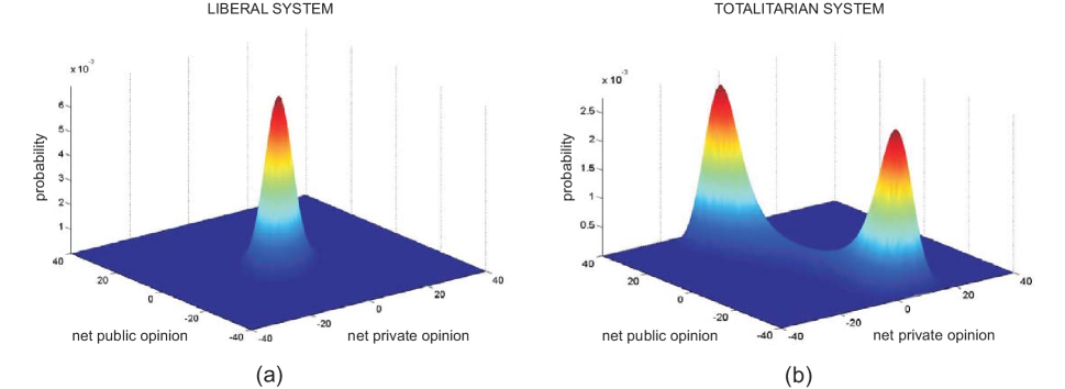
Figure 3: The joint probability distributions of the net public and private opinions in the liberal and totalitarian systems of opinion formation example of Section IV-I at steady-state computed by the KSA method. (a) The liberal system is characterized by a unimodal stationary distribution with its mode located at the point of zero net public and private opinions. (b) The totalitarian system is characterized by a bimodal stationary distribution with the modes corresponding to two different totalitarian states: one in which a large number of individuals publicly support the ideology of the ruling party, while a small number of individuals are privately against this ideology, and one in which a large number of individuals are publicly opposing the current ruling ideology, while a small number of individuals privately support it. In the latter case, the ruling party effectively switches its current ideology to fit public opinion, thus maintaining itself in power.

10. The MA method is based on replacing the mean value $\text{E}[\alpha_{m}(\boldsymbol{Z}(t))]$ by $\alpha_{m}(\boldsymbol{\mu}_{\scriptscriptstyle\boldsymbol{Z}}(t))+T_{m}(\boldsymbol{\mu}_{\scriptscriptstyle\boldsymbol{Z}}(t))$, where $T_{m}$ is a term calculated by solving differential equations for higher-order moments [see Eqs. (34)–(37)]. When the propensity function $\alpha_{m}(\boldsymbol{z})$ is convex, then Jensen’s inequality implies that $\text{E}[\alpha_{m}(\boldsymbol{Z}(t))]\geq\alpha_{m}(\text{E}[\boldsymbol{Z}(t)])=\alpha_{m}(\boldsymbol{\mu}_{\scriptscriptstyle\boldsymbol{Z}}(t))$. As a consequence, we must have $T_{m}(\boldsymbol{\mu}_{\scriptscriptstyle\boldsymbol{Z}}(t))\geq 0$, since $\text{E}[\alpha_{m}(\boldsymbol{Z}(t))]=\alpha_{m}(\boldsymbol{\mu}_{\scriptscriptstyle\boldsymbol{Z}}(t))+T_{m}(\boldsymbol{\mu}_{\scriptscriptstyle\boldsymbol{Z}}(t))\geq\alpha_{m}(\boldsymbol{\mu}_{\scriptscriptstyle\boldsymbol{Z}}(t))$. This however may not necessarily be the true, in which case the method may result in additional errors that can lead to instabilities. To address this problem, we can replace $\text{E}[\alpha_{m}(\boldsymbol{Z}(t))]$ with $\alpha_{m}(\boldsymbol{\mu}_{\scriptscriptstyle\boldsymbol{Z}}(t))+\max\{0,T_{m}(\boldsymbol{\mu}_{\scriptscriptstyle\boldsymbol{Z}}(t))\}$. In many instances, this simple modification results in a more accurate and more stable implementation of the MA method.

11. A moment closure scheme used in a particular application must produce moments that satisfy a number of necessary conditions. For example, all moments must be nonnegative and invariant under permutations. In addition, if $Z_{m_{1}}(t)$, $Z_{m_{2}}(t)$, and $Z_{m_{3}}(t)$ are mutually uncorrelated, then we must have $\text{E}[Z_{m_{1}}(t)Z_{m_{2}}(t)Z_{m_{3}}(t)]$ $=$ $\text{E}[Z_{m_{1}}(t)]\text{E}[Z_{m_{2}}(t)]\text{E}[Z_{m_{3}}(t)]$, whereas, if $Z_{m_{3}}(t)$ is uncorrelated from $Z_{m_{1}}(t)$ and $Z_{m_{2}}(t)$, we must have $\text{E}[Z_{m_{1}}(t)Z_{m_{2}}(t)Z_{m_{3}}(t)]$ $=$ $\text{E}[Z_{m_{1}}(t)]\text{E}[Z_{m_{2}}(t)Z_{m_{3}}(t)]$. Moreover, the resulting covariances must define a symmetric positive semi-definite matrix.

12. The assumptions underlying a given moment closure scheme may be inconsistent with the statistics of a particular reaction network at hand. In this case, the moment equations may have no solution, may produce a number of unrealistic solutions, or result in unstable and unbounded solutions Nåsell (2003b, a). Just like the LNA method, normal MA techniques cannot characterize bimodality or highly skewed probability distributions and may result in undesirable negative DA and population values Krishnarajah et al. (2005). Finally, much work must be done to determine conditions for the stability of the differential equations obtained by MA methods.

IV.8 Example: Opinion formation

To illustrate and compare the previous methods for solving the master equation, we focus on the opinion formation model discussed in Section III-E. The simplicity of this model permits us to solve the underlying master equation using a numerical approach. On the other hand, the complexity introduced by the nonlinear nature of the propensity functions given by Eq. (9), allows us to illustrate some intricate behavior. We consider two parameterizations of the model corresponding to a liberal democracy and a totalitarian regime Weidlich (2006). In particular, we assume a social system of $80$ individuals (in which case $L=40$) and set the values of the specific probability rate constants associated with the reactions in Eq. (8) to $\kappa_{1}=1/2~{}\mbox{day}^{-1}\mbox{individual}^{-1}$ and $\kappa_{2}=1~{}\mbox{day}^{-1}\mbox{individual}^{-1}$.

The main difference between the two social systems under consideration is that, in the liberal system, there is no pressure inflicted on public opinion with individuals having an affirmative private bias towards the ideology of the ruling party. On the other hand, there is heavy pressure in the totalitarian system inflicted on public opinion with individuals having a weakly dissident private opinion bias against the ruling ideology. We quantify these differences by setting $a_{1}=0~{}\mbox{individual}^{-1}$ and $a_{3}=1/80~{}\mbox{individual}^{-1}$ in the liberal system, and $a_{1}=3/80~{}\mbox{individual}^{-1}$, $a_{3}=-1/320~{}\mbox{individual}^{-1}$ in the totalitarian system. In addition, we assume that the two systems differ on how strongly privately held beliefs influence publicly stated opinions and set $a_{2}=1/80~{}\mbox{individual}^{-1}$ in the liberal system and $a_{2}=1/40~{}\mbox{individual}^{-1}$ in the totalitarian system. Finally, we consider the condition $X_{1}(0)=X_{2}(0)=0$, which represents completely neutral initial net publicly and privately held opinions.

We can numerically solve the master equation associated with the opinion formation model by employing the KSA method. This method is more appropriate than the IE method, since the DAs of the underlying reactions can grow rapidly in this case, whereas the populations $X_{1}(t)$ (net public opinion) and $X_{2}(t)$ (net private opinion) are bounded, taking values between $-40$ and $40$. To implement the KSA method, we used a Krylov subspace of dimension $K_{0}=40$. The joint probability distributions of the net public and private opinions in the liberal and totalitarian systems at steady-state are depicted in Fig. 3, whereas, movies encapsulating the entire dynamic evolutions of these distributions for a period of $15$ days can be found in the accompanying Matlab software. Evaluation of each solution took about $15$ seconds of CPU time on a 2.20 GHz Intel Core 2 Duo processor running Windows 7.

In the liberal system, the stationary joint probability distribution of public and private opinions is unimodal and almost identical to a sampled normal distribution; see Fig. 3(a). This distribution characterizes the fact that there is no need for an individual to hide her private opinion (thus the high correlation between the public and private opinions). As a consequence, the net opinions nearly balance around the origin, which represents an equal number of privately held and publicly pronounced opinions for or against the ruling ideology. On the other hand, the stationary joint probability distribution of public and private opinions in the totalitarian system is bimodal; see Fig. 3(b). Here, weakly dissident individuals tend to privately disapprove the ruling ideology, but pressure on public opinion ensures that most individuals publicly approve this ideology. As a consequence, dissidence is not strong enough to destabilize the totalitarian state and the system will operate around the peak located at point $(30,-6)$ with strong net public opinion in support of the ruling ideology and a rather weak private opinion against this ideology.

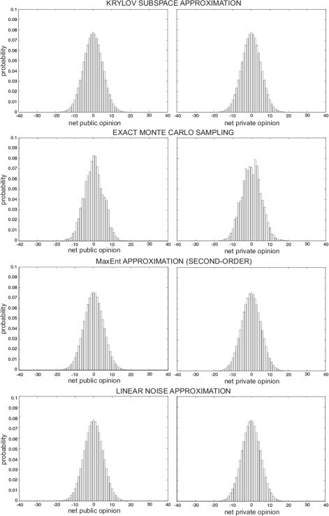
Figure 4: The stationary marginal probability distributions of the net public and private opinions in the liberal system of opinion formation example of Section IV-I computed by the Krylov subspace approximation method, exact Monte Carlo sampling, second-order MaxEnt approximation, and the lineal noise approximation method.

A totalitarian society may move to another peak located at point $(-30,6)$ with strong net public opinion against the ruling ideology and a rather weak private opinion in support of this ideology. This situation can be easily remedied by the ruling party, which can effectively change its ideology to fit the prevailing public opinion, thus preventing public upheaval and subsequent removal of the totalitarian regime from power.

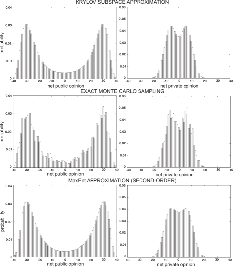
Figure 5: The stationary marginal probability distributions of the net public and private opinions in the totalitarian system of opinion formation example of Section IV-I, computed by the Krylov subspace approximation method, exact Monte Carlo sampling, and eighth-order MaxEnt approximation.

Finally, the dynamic evolutions of the joint probability distributions provided in the supplemental files demonstrate a rapid convergence of the liberal system to its stable stationary mode after $3$ days and a slower convergence of the totalitarian system to one of its two modes after $14$ days.

Instead of using the KSA method, we can estimate the probability distributions of the liberal and totalitarian systems by Monte Carlo sampling. To do so, we employ $4,\!000$ trajectories obtained from the master equation using the exact sampling algorithm of Gillespie at a cost of about $230$ seconds of CPU time. We depict the estimated stationary marginal probability distributions of the net public and private opinions in Fig. 4 for the liberal system, and in Fig. 5 for the totalitarian system. For comparison, we also depict the stationary marginal probability distributions obtained by the KSA method.

These results demonstrate the power and weakness of Monte Carlo estimation. Monte Carlo sampling is a simple and robust approach for solving the master equation which, in principle, allows us to compute almost any statistical summary of interest with arbitrary precision. The probability of a particular event can be estimated by counting the number of occurrences of the event and dividing by the total number of sampled trajectories. However, this simple and elegant procedure comes with a large computational cost, since the number of trajectories required to obtain a sufficiently accurate estimate is usually very large. Even for estimating the univariate marginal probability distributions of the net public and private opinions, $4,\!000$ iterations does not seem to be sufficient, since the symmetric and bimodal nature of these distributions can be obscured by estimation errors. As a matter of fact, it is often very difficult to know a priori how many samples must be used to sufficiently estimate the qualitative and quantitative properties of a statistical summary of interest or to verify a posteriori when convergence has occurred. Note however that the Monte Carlo method scales far better than the KSA method, since trajectories can be sampled from the master equation with a relative ease, even in the case of large Markovian reaction networks for which numerical methods, such as the KSA or IE methods, cannot be used. For large systems, the number of trajectories that can be sampled from the master equation in a reasonable time will certainly not be adequate for accurately computing complex population statistics, such as probability distributions, but they may be sufficient for estimating certain moments (e.g., the means and covariances) of the DA and population processes with a desired precision.

To ameliorate the computational burden of exact Monte Carlo sampling, we can employ a Langevin or Poisson approximation. Sampling $4,\!000$ trajectories from the master equation governing the opinion formation model using the LA method took $30$ seconds of CPU time, whereas, drawing the same number of samples using the PA method required $75$ seconds of CPU time. The estimation results are very similar to the ones obtained by exact Monte Carlo sampling (data not shown). The LA method however does not retain the integer-valued nature of the net opinion trajectories, which can be an issue when accurate simulation of these trajectories is desired.

By using the PA method, we can draw $4,\!000$ samples from the master equation and use these samples to estimate the first $K$ moments of the opinion trajectories under consideration. We can then use the MaxEnt method discussed in Section IV-C-5 to derive an analytical approximation of the marginal probability distributions of the net public and private opinions. The resulting sampled probability density functions depicted in Figs. 4 and 5 clearly show the potential of the MaxEnt method for correctly estimating the stationary marginal distributions in the opinion formation model. It took about $75$ seconds of CPU time to compute these results, which have been obtained by using the Matlab code developed by Mohammad-Djafari (1991). For the democratic system, we only need to estimate the first- and second-order moments by Monte Carlo. This is due to the fact that the true stationary distributions are almost sampled normal. On the other hand, to obtain sufficiently accurate approximations of the stationary marginal distributions in the totalitarian system, we need to estimate the first eight moments by Monte Carlo. The main advantage of MaxEnt is its ability to provide a relatively accurate approximation of marginal probability distributions by using appreciably fewer sample trajectories than the ones required by Monte Carlo in order to achieve a similar level of estimation accuracy.

Application of the LNA method for solving the master equation associated with the totalitarian system is not possible due to the bimodal nature of the stationary joint probability distribution (see Remark IV-G-7). This method however can be used in the case of the liberal system by choosing the system size parameter $\Omega$ to be equal to the “size” $L$ of the net public or private opinions. Evaluation of the solution obtained by the LNA method took only $0.35$ seconds of CPU time. The resulting Gaussian probability density function approximates well the stationary solution found by the KSA method. The sampled computed stationary marginal probability distributions of the net public and private opinions are depicted in Fig. 4. If there were more individuals in the system (i.e., for larger values of $\Omega$), then the LNA method could produce a more accurate result. On the other hand, a significantly smaller number of individuals may dramatically reduce the accuracy of the method, since the statistical properties of the system may appreciably deviate from normality. Despite its clear computational advantage, use of the LNA method is hampered by the absence of a strategy to effectively determine for which values of $\Omega$ the resulting normal approximation is accurate.

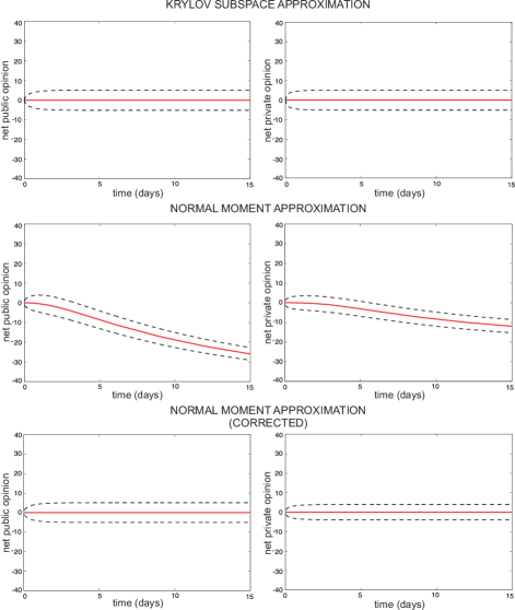
Figure 6: The means (solid red lines) and the $\pm 1$ standard deviations (dashed lines) of the net public and private opinions in the liberal system of opinion formation example of Section IV-I, obtained by the Krylov subspace and normal moment approximation methods (with and without correction using Jensen’s inequality).

Finally, use of the MA method is much easier for the liberal system than the totalitarian system, since the totalitarian system requires at least eighth-order moments to sufficiently characterize its bimodal stationary distribution. For simplicity, we will therefore focus on the liberal system. Note that, due to the exponential nature of the propensity functions, given by Eq. (9), their effect on the moment equations can persist through infinitely many derivatives, which can make the task of finding an appropriate moment closure scheme very difficult. However, since the stationary joint probability distributions of the net public and private opinions approximate well a sampled Gaussian distribution (see Fig. 4), we may be able to approximate the means and covariances by using the normal MA scheme given by Eqs. (36) and (37). In Fig. 6, we depict the means (solid red lines) and the $\pm 1$ standard deviations (dashed lines) of the net public and private opinions, obtained with the normal MA method. Implementation of this method took a mere $0.6$ seconds of CPU time. For comparison, we also depict the corresponding moments and standard deviations obtained with the KSA method. Clearly, the normal MA method produces unsatisfactory results.

The main culprit here is the fact that Eqs. (36) and (37) were derived for quadratic propensity functions whose higher-order derivatives vanish, which along with the Gaussian assumption results in a decoupling of the means and covariances from higher-order central moments. In the democratic system, the Gaussianity assumption is approximately valid but errors accumulate, since Eqs. (36) and (37) neglect to account for non-vanishing higher-order derivatives of the propensity functions. We can however improve the closure scheme by using Jensen’s inequality (see Remark IV-G-10), due to the convexity of the propensity functions. The results depicted in Fig. 6 clearly demonstrate the effectiveness of this correction.

V Multiscale methods

As we discussed earlier in this review (see Section IV-C-6), the reactions in a Markovian reaction network may occur at different time scales, with slow reactions occurring infrequently and fast reactions firing numerous times between successive occurrences of slow reactions. This may appreciably increase the computational effort required to sample the master equation by Monte Carlo, which can make analysis of Markovian reaction networks very difficult to perform in practice. In this section, we discuss methods available to address this problem. The main idea is to eliminate the fast reactions by approximating the master equation with one that consists of only slow reactions.

V.1 Partitioning approximation

In many cases of interest, it is not important to know the detailed activities of fast reactions, since the dynamic evolution of the state of a Markovian reaction network may be mostly determined by the slow reactions. If that is true, we may be able to approximate the master equation by one that consists only of slow reactions. If a sufficiently accurate approximation of the master equation can be found in terms of slow reactions, then it can be used to appreciably reduce the computational complexity associated with Monte Carlo sampling. This is due to the fact that sampling slow reactions is appreciably more efficient than sampling fast reactions. This idea has led to the development of techniques for eliminating fast reactions, known as multiscale or partitioning approximation methods Haseltine and Rawlings (2002); Rao and Arkin (2003); Puchałka and Kierzek (2004); Cao et al. (2005b); E et al. (2005); Goutsias (2005); Haseltine and Rawlings (2005); Salis and Kaznessis (2005); Samant and Vlachos (2005); Ball et al. (2006); E et al. (2007); Mastny et al. (2007); Gómez-Uribe et al. (2008); Chevalier and El-Samad (2009); Crudu et al. (2009); Zeron and Santillán (2010); Cotter et al. (2011); Pahlajani et al. (2011); Bostani et al. (2012); Kang and Kurtz (2012); Thomas et al. (2012).

To illustrate the main steps underlying most multiscale approximation schemes, let us assume that the first $M_{s}$ reactions of a Markovian reaction network are slow, whereas, the remaining $M_{\!f}=M-M_{s}$ reactions are fast. We can then decompose the DA process $\boldsymbol{Z}(t)$ into two components, $\boldsymbol{Z}_{\!s}(t)$ and $\boldsymbol{Z}_{\!f}(t)$, with the first component corresponding to the slow reactions and the second corresponding to the fast reactions. In this case, Eq. (4) leads to the following master equation Goutsias (2005):

$$\frac{\partial p_{\boldsymbol{z}_{\!s}}(\boldsymbol{z}_{\!s};t)}{\partial t}~{}=\!\!\sum_{m\in\mathcal{M}_{\!s}}\!\!{\Bigl{\{}}\alpha_{m}(\boldsymbol{z}_{\!s}-\overline{{\bf e}}_{m};t)p_{\boldsymbol{z}_{\!s}}(\boldsymbol{z}_{\!s}-\overline{{\bf e}}_{m};t)$$

$$\hskip 62.59605pt-\>\alpha_{m}(\boldsymbol{z}_{\!s};t)p_{\boldsymbol{z}_{\!s}}(\boldsymbol{z}_{\!s};t){\Bigr{\}}},$$ (46)

for $t>0$, with

$$\alpha_{m}(\boldsymbol{z}_{\!s};t)\>:=\>\sum_{\boldsymbol{z}_{\!f}}\alpha_{m}(\boldsymbol{z}_{\!s},\boldsymbol{z}_{\!f})p_{\boldsymbol{z}_{\!f}\mid\boldsymbol{z}_{\!s}}(\boldsymbol{z}_{\!s},\boldsymbol{z}_{\!f};t),$$ (47)

for $m\in\mathcal{M}_{\!s}$, where $p_{\boldsymbol{z}_{\!s}}(\boldsymbol{z}_{\!s};t)$ is the marginal probability distribution over the DAs of the slow reactions, $p_{\boldsymbol{z}_{\!f}\mid\boldsymbol{z}_{\!s}}(\boldsymbol{z}_{\!s},\boldsymbol{z}_{\!f};t)$ is the conditional probability of the fast DAs at time $t$ given the DAs of the slow reactions, $\mathcal{M}_{\!s}:=\{1,2,\ldots,M_{s}\}$, and $\overline{{\bf e}}_{m}$ is a vector comprised of the first $M_{s}$ rows of $\boldsymbol{e}_{m}$ (the $m\text{-th}$ column of the $M\times M$ identity matrix).

According to Eq. (46), the DAs of the slow reactions follow a master equation that is similar to the one governing the entire Markovian reaction network, albeit with time-varying propensities. The fast reactions exert their influence on the slow reactions through the propensity functions given by Eq. (47), which are computed as the conditional means of the original propensity functions given the DAs of the slow reactions. As a consequence, if we can evaluate the mean propensity functions $\alpha_{m}(\boldsymbol{z}_{\!s};t)$, $m\in\mathcal{M}_{\!s}$, then we can efficiently simulate the stochastic evolutions of the DAs of the slow reactions by using the exact Gillespie algorithm, or any other appropriate technique, modified to account for the fact that the propensity functions are now time-dependent Rao and Arkin (2003); Haseltine and Rawlings (2002). Moreover, given that $\boldsymbol{Z}_{\!s}(t)=\boldsymbol{z}_{\!s}$, we can estimate the population process $X_{n}(t)$ by using the optimum mean-square estimate $\widehat{x}_{n}(t)$, given by [recall Eq. (3)]:

$$\widehat{x}_{n}(t)=\text{E}[X_{n}(t)\mid\boldsymbol{Z}_{\!s}(t)=\boldsymbol{z}_{\!s}]$$

$$=x_{0,n}+\!\!\!\sum_{m\in\mathcal{M}_{\!s}}\!\!s_{nm}z_{m}(t)+\!\!\!\!\sum_{m\in\mathcal{M}_{\!f}}\!\!s_{nm}\mu_{\scriptscriptstyle\boldsymbol{Z}}(m;t,\boldsymbol{z}_{\!s}),$$ (48)

for $n\in\mathcal{N}$, where $\mu_{\scriptscriptstyle\boldsymbol{Z}}(m;t,\boldsymbol{z}_{\!s}):=\text{E}[Z_{m}(t)\mid\boldsymbol{Z}_{\!s}(t)=\boldsymbol{z}_{\!s}]$, for $m\in\mathcal{M}_{\!f}$ $:=$ $\{M_{\!s}+1,M_{\!s}+2,\ldots,M\}$, is the mean DA of the $m\text{-th}$ fast reaction at time $t$, given the state $\boldsymbol{z}_{\!s}(t)$ of the slow reactions at $t$. Hence, we can replace the Markovian reaction network by a “slow” Markovian reaction subnetwork whose DA process is governed by Eqs. (46), (47) and whose population process is governed by Eq. (48).

Calculating the propensity functions $\alpha_{m}(\boldsymbol{z}_{\!s};t)$, $m\in\mathcal{M}_{\!s}$, and the means $\mu_{\scriptscriptstyle\boldsymbol{Z}}(m;t,\boldsymbol{z}_{\!s})$, $m\in\mathcal{M}_{\!f}$, requires knowledge of the conditional probability $p_{\boldsymbol{z}_{f}\mid\boldsymbol{z}_{s}}(\boldsymbol{z}_{s},\boldsymbol{z}_{f};t)$. It can be shown that, within the coarse time scale, the dynamic evolution of this probability is approximately governed by the following master equation Goutsias (2005):

$$\frac{\partial p_{\boldsymbol{z}_{\!f}\mid\boldsymbol{z}_{s}}(\boldsymbol{z}_{s},\boldsymbol{z}_{\!f};t)}{\partial t}$$

$$=\!\!\sum_{m\in\mathcal{M}_{\!f}}\!\!{\Bigl{\{}}\alpha_{m}(\boldsymbol{z}_{\!s},\boldsymbol{z}_{\!f}-\underline{{\bf e}}_{m})p_{\boldsymbol{z}_{\!f}\mid\boldsymbol{z}_{\!s}}(\boldsymbol{z}_{\!s},\boldsymbol{z}_{\!f}-\underline{{\bf e}}_{m};t)$$

$$\hskip 28.45274pt-\alpha_{m}(\boldsymbol{z}_{\!s},\boldsymbol{z}_{\!f})p_{\boldsymbol{z}_{f}\mid\boldsymbol{z}_{\!s}}(\boldsymbol{z}_{\!s},\boldsymbol{z}_{\!f};t){\Bigr{\}}},$$ (49)

for $t>0$, where $\underline{{\bf e}}_{m}$ is a vector comprised of the last $\mathcal{M}_{\!f}$ rows of $\boldsymbol{e}_{m}$, which includes only the fast reactions. This equation is derived by assuming that, within successive firings of slow reactions, the “slow” Markovian reaction subnetwork behaves like one with propensity functions that are not appreciably larger than zero, since it is very unlikely that a slow reaction will occur within that time scale.

It turns out that most multiscale approximation schemes currently available in the literature follow a similar approach by decomposing a Markovian reaction network into “slow” and “fast” Markovian subnetworks based on appropriately chosen variables. Although the method discussed above uses the DAs of individual reactions Haseltine and Rawlings (2002); Goutsias (2005); Salis and Kaznessis (2005), similar methods can be constructed using the net DAs of reversible reactions Haseltine and Rawlings (2005), or the populations of the underlying species Rao and Arkin (2003); Cao et al. (2005b); Samant and Vlachos (2005); Gómez-Uribe et al. (2008); Chevalier and El-Samad (2009); Zeron and Santillán (2010).

Unfortunately, solving the master equation of the “fast” reaction subnetwork [e.g., Eq. (49)] is as difficult as solving the master equation of the entire network. Moreover, evaluating the propensity functions of the “slow” subnetwork requires Monte Carlo estimation in general, which adds to computational complexity. To address these issues, a number of different approaches have been proposed in the literature, based on the techniques discussed in Section IV. For example, it has been assumed that, within successive firings of slow reactions, the fast reactions rapidly reach a stationary state whose probability does not depend on time $t$ Rao and Arkin (2003); Cao et al. (2005b); E et al. (2005); Haseltine and Rawlings (2005); Samant and Vlachos (2005); E et al. (2007); Gómez-Uribe et al. (2008); Zeron and Santillán (2010). In this case, we can set the right-hand-side of the master equation of the “fast” reaction subnetwork equal to zero and use a numerical technique (see Sec. IV-B) to calculate the desired stationary conditional probability of the “fast” variables given the “slow” variables. We can then evaluate the propensity functions of the “slow” reaction subnetwork either by direct summation Haseltine and Rawlings (2005); Cao et al. (2005b), if computationally feasible, or by Monte Carlo estimation Haseltine and Rawlings (2005).

Numerically solving the master equation of the “fast” reaction subnetwork may not be easy, especially for large subnetworks. Moreover, evaluating expectations by direct summation or Monte Carlo estimation can be computationally demanding. The main difficulty however with the previous approach is to verify that the “fast” reaction subnetwork reaches a stationary state, since there might be only a short induction time between successive firings of slow reactions during which convergence to steady-state may not occur.

We can avoid the previous problems by sampling the master equation of the “fast” reaction subnetwork using the exact Gillespie algorithm and evaluate the propensity functions of the “slow” reaction subnetwork by Monte Carlo estimation E et al. (2005, 2007); Samant and Vlachos (2005). Although this strategy is very general, requiring no additional assumptions other than the ones leading to Eqs. (46), (47), and (49), the embedded estimation step may require a large number of Monte Carlo samples, which can substantially increase computations.

Exact sampling of the master equation of the “fast” reaction subnetwork can be replaced by the Langevin Haseltine and Rawlings (2002, 2005); Salis and Kaznessis (2005) or the Poisson Puchałka and Kierzek (2004) approximations. Although this can speed-up sampling of the “fast” variables, it will not eliminate the need for evaluating the propensity functions of the “slow” reaction subnetwork using Monte Carlo estimation. Due to its discrete nature, the Poisson approximation may be more preferable than the Langevin approximation. However, for both approximations to be valid and computationally efficient, it is necessary to determine a value for the leaping parameter $\tau$ that is as large as possible while still ensuring that occurrences of fast reactions within a time interval $[t,t+\tau)$ do not appreciably affect the propensity functions. Intuitively speaking, finding such value may be possible due to the assumed futility of the fast reactions. In practice however this may not be easy. Note finally that the expected number of occurrences of each fast reaction during $[t,t+\tau)$ will be much larger than one, a condition that is required for the Langevin approximation to be valid.

The propensity functions of the “slow” reaction subnetwork can be approximated by using Eq. (47) and a Taylor series expansion, such as the one given by Eq. (33), of the propensity functions of the entire network around the means of the “fast” variables. This can be done by evaluating the conditional moments of the “fast” variables, given the values of the “slow” variables, thus eliminating the need for Monte Carlo estimation. If the propensity functions of the “slow” reaction subnetwork depend only linearly on the “fast” variables, then we only need to calculate the conditional means of these variables. On the other hand, if the “slow” propensity functions depend quadratically on “fast” variables, then we also need to calculate the conditional covariances. We can perform these calculations by employing a moment approximation scheme applied on the master equation of the “fast” reaction subnetwork Haseltine and Rawlings (2002); Rao and Arkin (2003); Cao et al. (2005b); Goutsias (2005); Haseltine and Rawlings (2005); Gómez-Uribe et al. (2008); Chevalier and El-Samad (2009). The accuracy of this approach however depends on the degree of nonlinearity of the network propensity functions in terms of the “fast” variables and the particular moment approximation scheme used.

Most multiscale approximation methods developed so far are based on a clear separation between fast and slow reactions. In reality however this may not be possible. For this reason, it may be more appropriate to develop techniques that involve more than two separate time scales. We refer the reader to E et al. (2005, 2007) and Harris and Clancy (2006) for two promising techniques along this direction.

We should finally point out that a few alternative multiscale approximation schemes have been proposed in the literature, namely two techniques related to the finite state projection method Peleš et al. (2006); Pigolotti and Vulpiani (2008), a method based on separating species in terms of their variance Hellander and Lötstedt (2007), a technique based on an adiabatic approximation using a stochastic path integral Sinitsyn et al. (2009), and a rigorous and versatile technique based primarily on stochastic equations determining the dynamic evolution of the population process itself Ball et al. (2006); Kang and Kurtz (2012). Although promising, these methods have only been applied to very small reaction networks. At this point, it is not clear how they will perform when dealing with larger and more realistic networks, nor have they been sufficiently compared to the other approaches discussed in this section.

V.2 Example: Transcription regulation

To illustrate the effectiveness of a multiscale approximation method for solving the master equation, we consider here a biochemical reaction network comprised of six molecular species that interact through the following ten reactions:

$$\begin{array}[]{lrcl}\text{reaction}~{}1:{}{}&X_{1}&\rightarrow&X_{1}+X_{2}\\[2.0pt] \text{reaction}~{}2:{}{}&2X_{2}&\rightarrow&X_{3}\\[2.0pt] \text{reaction}~{}3:{}{}&X_{3}&\rightarrow&2X_{2}\\[2.0pt] \text{reaction}~{}4:{}{}&X_{3}+X_{4}&\rightarrow&X_{5}\\[2.0pt] \text{reaction}~{}5:{}{}&X_{5}&\rightarrow&X_{3}+X_{4}\\[2.0pt] \text{reaction}~{}6:{}{}&X_{3}+X_{5}&\rightarrow&X_{6}\\[2.0pt] \text{reaction}~{}7:{}{}&X_{6}&\rightarrow&X_{3}+X_{5}\\[2.0pt] \text{reaction}~{}8:{}{}&X_{5}&\rightarrow&X_{1}+X_{5}\\[2.0pt] \text{reaction}~{}9:{}{}&X_{1}&\rightarrow&\emptyset\\[2.0pt] \text{reaction}~{}10:{}{}&X_{2}&\rightarrow&\emptyset.\end{array}$$

This reaction network was originally proposed by Goutsias (2005) and can serve as a model for a particular type of transcription regulation in single cells. As a matter of fact, reaction 1 can be used to model the translation of an mRNA molecule $X_{1}$ into a protein molecule $X_{2}$, whereas reactions 2 and 3 can be used to model dimerization of $X_{2}$ into $X_{3}$. On the other hand, reactions 4–7 can be used to model the binding of dimer $X_{3}$ on a gene $X_{4}$, assuming that the promoter of this gene has two binding sites for $X_{3}$, whereas, reaction 8 can be used to model the transcription of $X_{4}$ to mRNA molecules $X_{1}$, assuming that this process occurs when the promoter of $X_{4}$ is only bound by one dimer $X_{3}$. Finally, reactions 9 and 10 model degradation of the mRNA and protein molecules $X_{1}$ and $X_{2}$, respectively. Here, we slightly simplify the original model by assuming that the cell’s volume remains fixed at $10^{-15}$ liters (l). In this case, the specific probability rate constants are set to $\kappa_{1}=0.043~{}\text{s}^{-1}$, $\kappa_{2}=0.083~{}\mbox{moles}\cdot\mbox{l}^{-1}\cdot\text{s}^{-1}$, $\kappa_{3}=0.5~{}\text{s}^{-1}$, $\kappa_{4}=0.0199~{}\mbox{moles}\cdot\mbox{l}^{-1}\cdot\text{s}^{-1}$, $\kappa_{5}=0.4791~{}\text{s}^{-1}$, $\kappa_{6}=1.9926\times 10^{-4}~{}\mbox{moles}\cdot\mbox{l}^{-1}\cdot\text{s}^{-1}$, $\kappa_{7}=8.7658\times 10^{-12}~{}\text{s}^{-1}$, $\kappa_{8}=0.0715~{}\text{s}^{-1}$, $\kappa_{9}=0.0039~{}\text{s}^{-1}$, and $\kappa_{10}=0.0007~{}\text{s}^{-1}$, in agreement with the values used by Goutsias (2005). Finally, we initialize the system by setting $X_{1}(0)=0$, $X_{2}(0)=2$, $X_{3}(0)=4$, $X_{4}(0)=2$, and $X_{5}(0)=X_{6}(0)=0$; i.e., we assume that the system contains initially two mRNA molecules, two copies of the same gene, and four dimers.

Despite the modest size of the previous network, simulation using exact Monte Carlo sampling of the master equation is computationally intensive. It took about $2$ hours and $15$ minutes of CPU time on a 2.20 GHz Intel Core 2 Duo processor running Windows 7 to obtain $2,\!000$ samples of the population dynamics during a period of $35$ minutes. This serious inefficiency is due to the stiffness of the system caused by the reversible reactions associated with the dimerization of protein $X_{2}$ (i.e., reactions 2 and 3) being much faster than the remaining reactions. As a consequence, exact Monte Carlo sampling is forced to spend a substantial amount of time simulating the occurrences of these two reactions. Unfortunately, we cannot appreciably reduce computational effort by using the Poisson approximation since, for accurately solving the master equation, stiffness constrains the leaping parameter $\tau$ to take a very small value thus deeming this approximation method computationally comparable to exact sampling. Dimerization however is reversible and occurs on a much faster timescale than the other reactions. As a consequence, we expect its effect to largely cancel out. Therefore, faithful simulation of dimerization may not be necessary.

If we set $\mathcal{M}_{s}=\{1,4,5,6,7,8,9,10\}$ and $\mathcal{M}_{f}=\{2,3\}$, then the “slow” subsystem, comprised of the reactions in $\mathcal{M}_{s}$, will be characterized by the master equation (46) with propensity functions given by [recall Eq. (47)]

$$\alpha_{1}(\boldsymbol{z}_{\!s};t) \!\!=\!\! \kappa_{1}(z_{8}-z_{9}),$$

$$\alpha_{4}(\boldsymbol{z}_{\!s};t) \!\!=\!\! \kappa_{4}[4-z_{4}+z_{5}-z_{6}+z_{7}+\mu_{\scriptscriptstyle\boldsymbol{Z}}(2;t,\boldsymbol{z}_{\!s})$$

$$\hskip 28.45274pt-\mu_{\scriptscriptstyle\boldsymbol{Z}}(3;t,\boldsymbol{z}_{\!s})](2-z_{4}+z_{5}),$$

$$\alpha_{5}(\boldsymbol{z}_{\!s};t) \!\!=\!\! \kappa_{5}(z_{4}-z_{5}-z_{6}+z_{7}),$$

$$\alpha_{6}(\boldsymbol{z}_{\!s};t) \!\!=\!\! \kappa_{6}[4-z_{4}+z_{5}-z_{6}+z_{7}+\mu_{\scriptscriptstyle\boldsymbol{Z}}(2;t,\boldsymbol{z}_{\!s})$$

$$\hskip 28.45274pt-\mu_{\scriptscriptstyle\boldsymbol{Z}}(3;t,\boldsymbol{z}_{\!s})](z_{4}-z_{5}-z_{6}+z_{7}),$$

$$\alpha_{7}(\boldsymbol{z}_{\!s};t) \!\!=\!\! \kappa_{7}(z_{6}-z_{7}),$$

$$\alpha_{8}(\boldsymbol{z}_{\!s};t) \!\!=\!\! \kappa_{8}(z_{4}-z_{5}-z_{6}+z_{7}),$$

$$\alpha_{9}(\boldsymbol{z}_{\!s};t) \!\!=\!\! \kappa_{9}(z_{8}-z_{9}),$$

$$\alpha_{10}(\boldsymbol{z}_{\!s};t) \!\!=\!\! \kappa_{10}[2\!+\!z_{1}\!-\!z_{10}\!-\!2\mu_{\scriptscriptstyle\boldsymbol{Z}}(2;t,\boldsymbol{z}_{\!s})\!+\!2\mu_{\scriptscriptstyle\boldsymbol{Z}}(3;t,\boldsymbol{z}_{\!s})],\vspace{-12pt}$$

where $\mu_{\scriptscriptstyle\boldsymbol{Z}}(2;t,\boldsymbol{z}_{\!s})$ and $\mu_{\scriptscriptstyle\boldsymbol{Z}}(3;t,\boldsymbol{z}_{\!s})$ are the mean DAs of the two fast reactions 2 and 3, respectively. Therefore, to calculate these propensities, we need to compute the difference $\mu_{\scriptscriptstyle\boldsymbol{Z}}(2;t,\boldsymbol{z}_{\!s})-\mu_{\scriptscriptstyle\boldsymbol{Z}}(3;t,\boldsymbol{z}_{\!s})$. By assuming that the “fast” reaction subsystem of the two dimerization reactions rapidly reaches equilibrium within successive occurrences of slow reactions, we can show that [see Goutsias (2005)]

$$\mu_{\scriptscriptstyle\boldsymbol{Z}}(2;t,\boldsymbol{z}_{\!s})-\mu_{\scriptscriptstyle\boldsymbol{Z}}(3;t,\boldsymbol{z}_{\!s})\!=\!\frac{1}{2}{\Big{[}}A(\boldsymbol{z}_{\!s})\!-\!\sqrt{A^{2}(\boldsymbol{z}_{\!s})-4B(\boldsymbol{z}_{\!s})}{\Big{]}}\!,$$ (50)

where

$$\begin{array}[]{ll}A(\boldsymbol{z}_{\!s})=1.5+z_{1}-z_{10}+(\kappa_{3}/2\kappa_{2})\\[6.0pt] B(\boldsymbol{z}_{\!s})=0.25(1+z_{1}-z_{10})(2+z_{1}-z_{10})\\ ~{}~{}~{}~{}~{}~{}~{}~{}~{}~{}~{}~{}~{}-(\kappa_{3}/2\kappa_{2})(4-z_{4}+z_{5}-z_{6}+z_{7}).\end{array}$$ (51)

As a consequence, we can solve the master equation (46) of the “slow” reaction subsystem without having to solve the conditional master equation (49) of the “fast” subsystem, and estimate the population process by using Eq. (48), which depends only on the difference $\mu_{\scriptscriptstyle\boldsymbol{Z}}(2;t,\boldsymbol{z}_{\!s})-\mu_{\scriptscriptstyle\boldsymbol{Z}}(3;t,\boldsymbol{z}_{\!s})$, and Eqs. (50), (51).

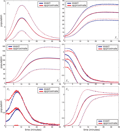
Figure 7: Means (solid lines) and $\pm 1$ standard deviations (dashed lines) of the population processes in the transcription regulation network example of Section V-B obtained by exact Monte Carlo sampling (blue lines) and multiscale approximation (red lines).

It took less than a minute ($52$ seconds) of CPU time to draw $2,\!000$ Monte Carlo samples from the master equation of the “slow” reaction subsystem (as compared to $135$ minutes of CPU time required by exact Monte Carlo sampling). The mean and $\pm 1$ standard deviation dynamics of the underlying population processes obtained by the two methods are depicted in Fig. 7. These results clearly show that an appropriately derived multiscale approximation of a stiff Markovian reaction network can lead to dramatic improvements in computational efficiency while producing a relatively accurate approximation of the population dynamics. It turns out that the relatively large transient errors in the population dynamics of $X_{4}$ and $X_{5}$ depicted in Fig. 7 are due to incorrectly computing the net DA $Z(4)-Z(5)$ of reactions 4 and 5 (binding and unbinding of dimer $X_{3}$ on the promoter of gene $X_{4}$), which is a consequence of the imposed adiabatic approximation of the DAs of the fast reactions 2 and 3 (dimerization) through their mean values. Although this approximation also affects the accuracy of the remaining population dynamics, the resulting approximate dynamics track the ones computed by exact Monte Carlo sampling sufficiently well.

VI Mesoscopic (probabilistic) behavior

An important goal when studying Markovian reaction networks is to investigate the existence, uniqueness, and stability of a stationary solution of the underlying master equation and derive mathematical properties of the dynamic behavior of the probability distribution of the system state. This can be done by using a mesoscopic description of the network in terms of the population probabilities $\{p_{\scriptscriptstyle\boldsymbol{X}}(\boldsymbol{x};t),\boldsymbol{x}\in\mathcal{X}\}$, for $t\geq 0$. To avoid mathematical subtleties, which are outside the scope of this review, we assume here that the cardinality of the population state-space $\mathcal{X}$ is finite. Most results however can be extended to the case of countable state-spaces.

To derive a stationary solution of the master equation (5), we must solve the system of $K$ linear equations $\mathbb{P}\boldsymbol{p}=0$; recall Eq. (20). Since the elements of each column of matrix $\mathbb{P}$ add to zero, its rows are linearly dependent and, therefore, the rank of $\mathbb{P}$ will be less than $K$. As a consequence, $\mathbb{P}\boldsymbol{p}=0$ will have at least one nontrivial solution. Unfortunately, this result does not tell us how many nontrivial solutions exist and which ones are valid probability distributions; i.e., which solutions satisfy the necessary constraints

$$0\leq p_{k}\leq 1,~{}~{}\mbox{for $k=1,2,\ldots,K$},~{}~{}\mbox{and}~{}~{}\sum_{k=1}^{K}p_{k}=1.$$

In the following, we first consider the dynamic behavior of an irreducible Markovian reaction network. This type of network is defined by the property that, for any pair $(\boldsymbol{x},\boldsymbol{x}^{\prime})$ of population states, there exists at least one sequence of reactions that takes the system from state $\boldsymbol{x}$ to state $\boldsymbol{x}^{\prime}$ – these states are said to be communicating. By using a simple graph theoretic analysis and Kirchhoff’s theorem, Schnakenberg (1976) has shown that an irreducible Markovian reaction network converges to a unique probability distribution $\overline{\boldsymbol{p}}$ at steady-state, which does not depend on the initial probability distribution $\boldsymbol{p}(0)$, such that $0<\overline{\boldsymbol{p}}<1$ [see also van Kampen (2007)]. As a consequence, in an irreducible Markovian reaction network, the population process can take any value in $\mathcal{X}$ at steady-state with nonzero probability.

On the other hand, the theory of systems of ordinary differential equations with constant coefficients implies that, for a given initial probability distribution $\boldsymbol{p}(0)$, Eq. (20) is satisfied by a unique probability distribution $\boldsymbol{p}(t)$, $t>0$, which is analytic for all $0\leq t<\infty$. Since the elements of each column of matrix $\mathbb{P}$ add to zero,

$$\frac{d[\boldsymbol{e}^{T}\boldsymbol{p}(t)]}{dt}=\boldsymbol{e}^{T}\frac{d\boldsymbol{p}(t)}{dt}=\boldsymbol{e}^{T}\mathbb{P}\>\boldsymbol{p}(t)=0,$$

where $\boldsymbol{e}$ is a $K\times 1$ vector with all its elements being equal to one. This result, together with the fact that $\boldsymbol{e}^{T}\boldsymbol{p}(0)=1$, implies $\boldsymbol{e}^{T}\boldsymbol{p}(t)=1$, for all $t\geq 0$. Unfortunately, it is not clear whether $0\leq\boldsymbol{p}(t)\leq 1$, for every $t>0$. It turns out however that, for an irreducible Markovian reaction network, $0<\boldsymbol{p}(t)<1$, for every $t>0$ Schnakenberg (1976).

If $\lambda_{k}$, $k=1,2,\ldots,K$, are the eigenvalues of matrix $\mathbb{P}$, with corresponding right and left eigenvectors $\boldsymbol{r}_{k}$, $\boldsymbol{l}_{k}$, $k=1,2,\ldots,K$, respectively, then the solution to Eq. (20) is given by Moler and van Loan (2003)

$${\boldsymbol{p}}(t)=\exp\left(\mathbb{P}t\right)\boldsymbol{p}(0)=\sum_{k=1}^{K}c_{k}\>\boldsymbol{r}_{k}\>e^{\lambda_{k}t},$$ (52)

for $0\leq t\leq\infty$, where we assume here that the eigenvalues of $\mathbb{P}$ have the same algebraic and geometric multiplicity, an assumption satisfied by many Markovian reaction networks. In this case, the right and left eigenvectors are biorthogonal (i.e., $\boldsymbol{l}^{T}_{k}\boldsymbol{r}_{k^{\prime}}=0$, for every $k\not=k^{\prime}$), which implies that the constants $c_{k}$ are given by $c_{k}=\boldsymbol{l}_{k}^{T}{\boldsymbol{p}(0)}/\boldsymbol{l}_{k}^{T}\boldsymbol{r}_{k}$. As a consequence, we can use the eigenvalues and eigenvectors of $\mathbb{P}$ to analytically specify the entire mesoscopic behavior of a Markovian reaction network. See Keeling and Ross (2008) and Vellela and Qian (2009) for application of Eq. (52) to problems in epidemiology and computational biochemistry.

Note that Eq. (52) and the fact that a non-trivial stationary solution always exists imply that at least one eigenvalue of $\mathbb{P}$ must be zero. For an irreducible Markovian reaction network, matrix $\mathbb{P}$ has only one zero eigenvalue, with the remaining $K-1$ eigenvalues having negative real parts Schnakenberg (1976). If we therefore assume that $\lambda_{1}=0$, then Eq. (52) implies that the stationary distribution will be given by $\overline{{\boldsymbol{p}}}=\boldsymbol{r}_{1}/\|\boldsymbol{r}_{1}\|$, where $\boldsymbol{r}_{1}$ is the eigenvector corresponding to the zero eigenvalue and $\|\boldsymbol{r}\|$ is the $\ell_{1}$-norm of vector $\boldsymbol{r}$. It turns out that the solution $\boldsymbol{p}(t)$, $t\geq 0$, of Eq. (20) is asymptotically stable with respect to $\overline{\boldsymbol{p}}$, in the sense that

$$\lim_{t\rightarrow\infty}D[\boldsymbol{p}(t),\overline{\boldsymbol{p}}]=0,$$

where

$$D[\boldsymbol{p},\boldsymbol{q}]:=\sum_{k=1}^{K}p_{k}\ln\frac{p_{k}}{q_{k}}$$ (53)

is the Kullback-Leibler distance between the two probability distributions $\boldsymbol{p}=\{p_{k},k=1,2,\ldots,K\}$ and $\boldsymbol{q}=\{q_{k},k=1,2,\ldots,K\}$. As a matter of fact, $dD[\boldsymbol{p}(t),\overline{\boldsymbol{p}}]/dt\leq 0$, where equality is archived only at steady-state.

To summarize, for a given initial probability vector $\boldsymbol{p}(0)$, the master equation associated with an irreducible Markovian reaction network has a unique and strictly positive solution $0<\boldsymbol{p}(t)<1$, $0<t\leq\infty$. This solution is analytic for all $0\leq t<\infty$, converges to a stationary distribution $0<\overline{\boldsymbol{p}}<1$ that does not depend on the initial probability distribution $\boldsymbol{p}(0)$, and is asymptotically stable with respect to $\overline{\boldsymbol{p}}$.

It is not in general easy to check whether a Markovian reaction network is irreducible. However, we often assume that a given Markovian reaction network is comprised of only reversible reactions (reactions which can occur in both directions with nonzero probability). This is a plausible assumption since, in principle, a transition between two physical states can occur in the reverse direction as well. In this case, and after appropriately ordering the states, matrix $\mathbb{P}$ can be cast into a block diagonal form with diagonal elements $\mathbb{P}^{(1)},\mathbb{P}^{(2)},\ldots,\mathbb{P}^{(J)}$, for some $J$, where each submatrix $\mathbb{P}^{(j)}$ is irreducible (when $J=1$, matrix $\mathbb{P}$ is itself irreducible). The resulting Markovian reaction network is said to be completely reducible van Kampen (2007). In this case, the original Markovian reaction network can be decomposed into $J$ non-interacting subnetworks with non-overlapping state-spaces, which can be treated independently of each other. Each reaction subnetwork is characterized by unique dynamic and stationary solutions $\boldsymbol{p}^{(j)}(t)$, $\overline{\boldsymbol{p}}^{(j)}$, $j=1,2,\ldots,J$, that satisfy the aforementioned properties. However, the dynamic and stationary solutions of the original master equation are determined by the initial condition at time $t=0$. If the master equation is initialized with a population vector in the state-space of the $j\text{-th}$ subnetwork, then its dynamic and stationary solution will be given by

$$\left[\begin{array}[]{c}{\bf 0}\\ \vdots\\[6.0pt] {\boldsymbol{p}}^{(j)}(t)\\ \vdots\\ {\bf 0}\end{array}\right]\qquad\mbox{and}\qquad\left[\begin{array}[]{c}{\bf 0}\\ \vdots\\[6.0pt] \overline{{\boldsymbol{p}}}^{(j)}\\ \vdots\\ {\bf 0}\end{array}\right],$$

respectively, where ${\boldsymbol{p}}^{(j)}(t)$ depends on the initial condition and $\overline{{\boldsymbol{p}}}^{(j)}$ does not.

A question that arises at this point is what happens when the Markovian reaction network contains irreversible reactions and matrix $\mathbb{P}$ is not irreducible. To get an idea, let us assume that, after appropriately ordering the states,

$$\mathbb{P}=\left[\begin{array}[]{ll}\mathbb{P}^{(1)}&\mathbb{T}^{(1)}\\[6.0pt] {\bf 0}&\mathbb{T}^{(2)}\end{array}\!\!\right],$$

where $\mathbb{P}^{(1)}$ and $\mathbb{T}^{(2)}$ are square matrices, $\mathbb{P}^{(1)}$ is irreducible, and at least one element of each column of $\mathbb{T}^{(1)}$ is strictly positive. Note that the nonzero elements of $\mathbb{T}^{(1)}$ correspond to nonreversible reactions. The associated Markovian reaction network is said to be incompletely reducible van Kampen (2007). If we denote by ${\boldsymbol{p}}^{(1)}(t)$ and ${\boldsymbol{p}}^{(2)}(t)$ the probability distributions of the state vectors at time $t$, determined by the partition of the state-space suggested by matrix $\mathbb{P}$, then the master equation results in the following two differential equations:

$$\frac{d{\boldsymbol{p}}^{(1)}(t)}{dt} \!\!=\!\! \mathbb{P}^{(1)}{\boldsymbol{p}}^{(1)}(t)+\mathbb{T}^{(1)}{\boldsymbol{p}}^{(2)}(t)$$

$$\frac{d{\boldsymbol{p}}^{(2)}(t)}{dt} \!\!=\!\! \mathbb{T}^{(2)}{\boldsymbol{p}}^{(2)}(t).$$

Clearly, one can solve the second equation independently from the first to obtain

$${\boldsymbol{p}}^{(2)}(t)=\exp\!{\bigl{\{}}\mathbb{T}^{(2)}t{\bigr{\}}}\>{\boldsymbol{p}}^{(2)}(0).$$

On the other hand, the dynamic behavior of ${\boldsymbol{p}}^{(1)}$ is now driven by ${\boldsymbol{p}}^{(2)}(t)$, unless ${\boldsymbol{p}}^{(2)}(0)=0$, in which case ${\boldsymbol{p}}^{(1)}(t)=\exp\!{\bigl{\{}}\mathbb{P}^{(1)}t{\bigr{\}}}{\boldsymbol{p}}^{(1)}(0)$. Note however that

$$\frac{d[\boldsymbol{e}^{T}\boldsymbol{p}^{(2)}(t)]}{dt} \!\!=\!\! \boldsymbol{e}^{T}\frac{d\boldsymbol{p}^{(2)}(t)}{dt}$$

$$\!\!=\!\! \boldsymbol{e}^{T}\mathbb{T}^{(2)}{\boldsymbol{p}}^{(2)}(t)$$

$$\!\!=\!\! -\boldsymbol{e}^{T}\mathbb{T}^{(1)}{\boldsymbol{p}}^{(2)}(t)<0,$$

provided that ${\boldsymbol{p}}^{(2)}(t)\not={\bf 0}$, for every $t\geq 0$, since the elements of each column of matrix $\mathbb{P}$ add to zero and we have assumed that each column of matrix $\mathbb{T}^{(1)}$ contains at least one element that is strictly positive. Therefore, ${\boldsymbol{p}}^{(2)}(t)$ asymptotically becomes zero as $t\rightarrow\infty$. As a matter of fact, ${\boldsymbol{p}}^{(2)}(t)$ assigns probability mass over the transient states of the Markovian reaction network, as opposed to ${\boldsymbol{p}}^{(1)}(t)$ that assigns probability mass over the persistent states. In this case, and when matrix $\mathbb{P}^{(1)}$ is irreducible, the stationary solution of the master equation governing an incompletely reducible Markovian reaction network will be unique and given by the probability vector

$$\overline{{\boldsymbol{p}}}=\left[\begin{array}[]{l}\overline{{\boldsymbol{p}}}^{(1)}\\[6.0pt] {\bf 0}\end{array}\!\right],$$

where $\overline{{\boldsymbol{p}}}^{(1)}$ is the (unique) solution of the linear system of equations $\mathbb{P}^{(1)}{\boldsymbol{p}}={\bf 0}$.

In general, the population states in a Markovian reaction network can be classified into two distinct groups: transient and persistent. These states can be uniquely partitioned into non-overlapping sets $T$ and $P_{j}$, $j=1,2,\ldots,J$, where $T$ contains all transient states and $P_{j}$, $j=1,2,\ldots,J$, are irreducible sets containing persistent states with the additional property that, for every $j\not=j^{\prime}$, each state in $P_{j}$ does not communicate with any state in $P_{j^{\prime}}$. By appropriately ordering the states, we can write matrix $\mathbb{P}$ in the form

$$\mathbb{P}=\left[\begin{array}[]{ccccccc}\mathbb{P}^{(1)}&{\bf 0}&\cdot&\cdot&\cdot&{\bf 0}&\mathbb{T}^{(1)}\\[6.0pt] {\bf 0}&\mathbb{P}^{(2)}&\cdot&\cdot&\cdot&{\bf 0}&\mathbb{T}^{(2)}\\ \cdot&\cdot&\cdot&&&\cdot&\cdot\\[-3.0pt] \cdot&\cdot&&\cdot&&\cdot&\cdot\\[-3.0pt] \cdot&\cdot&&&\cdot&\cdot&\cdot\\ {\bf 0}&{\bf 0}&\cdot&\cdot&\cdot&\mathbb{P}^{(J)}&\mathbb{T}^{(J)}\\[6.0pt] {\bf 0}&{\bf 0}&\cdot&\cdot&\cdot&{\bf 0}&\mathbb{T}\end{array}\right],$$

where $\mathbb{P}^{(j)}$ is a square irreducible matrix that characterizes how probability mass is dynamically distributed among the persistent states in $P_{j}$, $\mathbb{T}^{(j)}$ is a matrix that tells us how probability mass is transferred from the transient states in $T$ to persistent states in $P_{j}$, and $\mathbb{T}$ is a square matrix that characterizes how probability mass is dynamically distributed among the transient states in $T$. In this case, if the Markovian reaction network is initialized by a persistent state in $P_{j}$, then the stationary solution will be given by the probability vector

$$\boldsymbol{g}_{j}=\left[\begin{array}[]{c}{\bf 0}\\ \cdot\\[-3.0pt] \cdot\\[-3.0pt] \cdot\\ \overline{{\boldsymbol{p}}}^{(j)}\\ \cdot\\[-3.0pt] \cdot\\[-3.0pt] \cdot\\ {\bf 0}\end{array}\!\right],$$

where $\overline{{\boldsymbol{p}}}^{(j)}$ is the unique stationary distribution of the $j\text{-th}$ irreducible Markovian reaction subnetwork characterized by matrix $\mathbb{P}^{(j)}$. However, if the network is initialized with the $i\text{-th}$ transient state in $T$, then the stationary distribution $\overline{\boldsymbol{p}}_{i}$ (which now depends on $i$) will be given by a convex combination of the stationary distributions $\boldsymbol{g}_{j}$ above, with mixing coefficients $\mu_{ij}$; i.e., we have that

$$\overline{\boldsymbol{p}}_{i}=\sum_{j=1}^{J}\mu_{ij}\boldsymbol{g}_{j},$$ (54)

where

$$\mu_{ij}\geq 0\qquad\mbox{and}\qquad\sum_{j=1}^{J}\mu_{ij}=1.$$

As a matter of fact, Eq. (54) simply expresses the fact that the probability of a Markovian reaction network initialized with the $i\text{-th}$ transient state in $T$ to reach a persistent population state $\boldsymbol{x}$ in $P_{j}$ at steady-state equals the probability $\mu_{ij}$ that the system will reach a persistent state in $P_{j}$ at steady-state multiplied by the probability that this state will be $\boldsymbol{x}$. It can be shown that

$$\mu_{ij}=-\sum_{i^{\prime}\in T}\sum_{j^{\prime}\in P_{j}}[\mathbb{T}^{(j)}]_{j^{\prime}i^{\prime}}[\mathbb{T}^{-1}]_{i^{\prime}i},$$

where $[\mathbb{T}^{(j)}]_{j^{\prime}i^{\prime}}$ is the $(j^{\prime},i^{\prime})$ element of matrix $\mathbb{T}^{(j)}$ and $[\mathbb{T}^{-1}]_{i^{\prime}i}$ is the $(i^{\prime},i)$ element of the inverse of matrix $\mathbb{T}$.

To summarize, a fundamental property of the master equation (5) associated with a Markovian reaction network is that, when this equation is initialized with a persistent state, its solution converges to a unique stationary distribution that assigns positive probability only to the persistent states that communicate with the initial state. On the other hand, if the Markovian reaction network is initialized with a transient state, then its stationary distribution will be a convex combination of the distinct stationary distributions obtained by initializing the system with persistent states chosen from each individual irreducible set.

VII Potential energy landscape

To better understand what might happen at steady-state, let us assume that the master equation (5) has a unique stationary solution $\overline{p}_{\scriptscriptstyle\bf X}(\boldsymbol{x}):=\lim_{t\rightarrow\infty}p_{\scriptscriptstyle\boldsymbol{X}}(\boldsymbol{x};t)$ that is independent of the initial state. The probability distribution $p_{\scriptscriptstyle\widetilde{\boldsymbol{X}}}(\widetilde{\boldsymbol{x}};t)$ of the population density process $\widetilde{\boldsymbol{X}}(t;\Omega)=\boldsymbol{X}(t)/\Omega$ will be given by $p_{\scriptscriptstyle\widetilde{\boldsymbol{X}}}(\widetilde{\boldsymbol{x}};t)=\Omega p_{\scriptscriptstyle\boldsymbol{X}}(\Omega\widetilde{\boldsymbol{x}};t)$ and will depend on the size parameter $\Omega$ in general. Let us define the function

$$V(\widetilde{\boldsymbol{x}};\Omega):=-\frac{1}{\Omega}\ln\frac{\overline{p}_{\scriptscriptstyle\widetilde{\boldsymbol{X}}}(\widetilde{\boldsymbol{x}})}{\overline{p}_{\scriptscriptstyle\widetilde{\boldsymbol{X}}}(\widetilde{\boldsymbol{x}}_{*})},$$ (55)

where $\overline{p}_{\scriptscriptstyle\widetilde{\boldsymbol{X}}}(\widetilde{\boldsymbol{x}}):=\lim_{t\rightarrow\infty}p_{\scriptscriptstyle\widetilde{\boldsymbol{X}}}(\widetilde{\boldsymbol{x}};t)$ is the steady-state distribution of the population density process and $\widetilde{\boldsymbol{x}}_{*}$ is a state at which the stationary probability distribution $\overline{p}_{\scriptscriptstyle\widetilde{\boldsymbol{X}}}(\widetilde{\boldsymbol{x}})$ attains its maximum value. Note that $V(\widetilde{\boldsymbol{x}};\Omega)\geq 0$. Moreover, and as a consequence of Eq. (55), we have that

$$\overline{p}_{\scriptscriptstyle\widetilde{\boldsymbol{X}}}(\widetilde{\boldsymbol{x}})=\frac{1}{\zeta(\Omega)}\exp{\Bigl{\{}}\!-\Omega V(\widetilde{\boldsymbol{x}};\Omega){\Bigr{\}}},$$ (56)

where

$$\zeta(\Omega):=\sum_{\boldsymbol{u}}\exp{\Bigl{\{}}\!-\Omega V(\boldsymbol{u};\Omega){\Bigr{\}}}.$$ (57)

In this case, $\overline{p}_{\scriptscriptstyle\widetilde{\boldsymbol{X}}}(\widetilde{\boldsymbol{x}})$ is a Gibbs distribution with “potential energy” function $V(\widetilde{\boldsymbol{x}};\Omega)$, “temperature” $1/\Omega$, and partition function $\zeta(\Omega)$. Clearly, $V(\widetilde{\boldsymbol{x}};\Omega)$ assigns minimum (zero) potential to the states of maximum probability at steady-state and infinite potential to the states of zero probability.

We will now assume that, around the thermodynamic limit, the potential function $V(\widetilde{\boldsymbol{x}};\Omega)$ is an analytic function of $\Omega^{-1}$. Then, a Taylor series expansion with respect to $\Omega^{-1}$ around zero (i.e., around the thermodynamic limit) results in

$$V(\widetilde{\boldsymbol{x}};\Omega) \!\!=\!\! V(\widetilde{\boldsymbol{x}};\infty)+\frac{1}{\Omega}\frac{\partial V(\widetilde{\boldsymbol{x}};\infty)}{\partial\Omega^{-1}}+\cdots$$ (58)

$$\!\!=\!\! V_{0}(\widetilde{\boldsymbol{x}})+\frac{1}{\Omega}V_{1}(\widetilde{\boldsymbol{x}})+\cdots,$$

where

$$V_{0}(\widetilde{\boldsymbol{x}}):=V(\widetilde{\boldsymbol{x}};\infty)=-\lim_{\Omega\rightarrow\infty}\frac{1}{\Omega}\ln\frac{\overline{p}_{\scriptscriptstyle\widetilde{\boldsymbol{X}}}(\widetilde{\boldsymbol{x}})}{\overline{p}_{\scriptscriptstyle\widetilde{\boldsymbol{X}}}(\widetilde{\boldsymbol{x}}_{0})}\geq 0,$$

and

$$V_{1}(\widetilde{\boldsymbol{x}}):=\frac{\partial V(\widetilde{\boldsymbol{x}};\infty)}{\partial\Omega^{-1}}.$$

As a consequence of Eqs. (56)–(58), and for sufficiently large $\Omega$, we have that

$$\overline{p}_{\scriptscriptstyle\widetilde{\boldsymbol{X}}}(\widetilde{\boldsymbol{x}})\simeq\frac{1}{\zeta(\Omega)}\exp{\Bigl{\{}}\!-\Omega V_{0}(\widetilde{\boldsymbol{x}})-V_{1}(\widetilde{\boldsymbol{x}}){\Bigr{\}}},$$

where the partition function is now given by

$$\zeta(\Omega)=\sum_{\boldsymbol{u}}\exp{\Bigl{\{}}\!-\Omega V_{0}(\boldsymbol{u})-V_{1}(\boldsymbol{u}){\Bigr{\}}}.$$

Therefore, the stationary probability distribution $\overline{p}_{\scriptscriptstyle\widetilde{\boldsymbol{X}}}(\widetilde{\boldsymbol{x}})$ satisfies a large deviation principle with rate function $V_{0}(\widetilde{\boldsymbol{x}})$ Touchette (2009). It turns out that, if $\boldsymbol{\chi}(t)$ satisfies the macroscopic equations (44), then

$$\frac{dV_{0}(\boldsymbol{\chi}(t))}{dt}=\sum_{n\in\mathcal{N}}\frac{\partial V_{0}(\boldsymbol{\chi}(t))}{\partial\chi_{n}(t)}\frac{d\chi_{n}(t)}{dt}\leq 0,$$

with equality if and only if

$$\frac{d\chi_{n}(t)}{dt}=0,\quad\mbox{for~{}every~{}$n\in\mathcal{N}$}.$$

Therefore, the solution $\boldsymbol{\chi}(t)$ of the macroscopic equation (44) produces a downhill motion in the value of the potential energy function $V_{0}$ (which is a Lyapunov function for the macroscopic system) until it asymptotically reaches a stable stationary state.

For a given value of $\Omega$, we can view the multidimensional surface $V_{0}(\widetilde{\boldsymbol{x}};\Omega)$ as a potential energy landscape Ao et al. (2007); Wang et al. (2008); Zhou and Qian (2011); Wang et al. (2011). The stable stationary states of Eq. (44) correspond to potential wells (basins of attraction) associated with the (local or global) minima of $V_{0}$, which are separated by barriers corresponding to hills (unstable states) and saddles (transitional states – states on the potential energy surface from which stable states are equally accessible). Which minimum will be reached depends on the initial condition that must be a point in the potential well of that minimum. It turns out that, once the macroscopic system, given by Eq. (44), reaches a stable stationary state, it will stays there forever. As a consequence, the macroscopic system will only move downhill on the potential energy landscape.

It is now not difficult to see that Eqs. (56)–(58) imply that

$$\lim_{\Omega\rightarrow\infty}\overline{p}_{\scriptscriptstyle\widetilde{\boldsymbol{X}}}(\widetilde{\boldsymbol{x}}) \!\!=\!\! \lim_{\Omega\rightarrow\infty}\frac{\exp{\Bigl{\{}}\!-\Omega V_{0}(\widetilde{\boldsymbol{x}}){\Bigr{\}}}\exp{\Bigl{\{}}\!-V_{1}(\widetilde{\boldsymbol{x}}){\Bigr{\}}}}{\sum_{\boldsymbol{u}}\exp{\Bigl{\{}}\!-\Omega V_{0}(\boldsymbol{u}){\Bigr{\}}}\exp{\Bigl{\{}}\!-V_{1}(\boldsymbol{u}){\Bigr{\}}}}$$ (61)

$$\!\!=\!\! \left\{\begin{array}[]{ll}{\displaystyle\frac{\exp\{-V_{1}(\widetilde{\boldsymbol{x}})\}}{\sum_{\boldsymbol{u}\in\mathcal{G}_{*}}\exp\{-V_{1}(\widetilde{\boldsymbol{u}})\}}},&~{}\mbox{if~{}~{}$\widetilde{\boldsymbol{x}}\in\mathcal{G}_{*}$}\\[12.0pt] ~{}~{}~{}~{}~{}~{}~{}~{}~{}~{}~{}0,&~{}\mbox{otherwise,}\end{array}\right.$$

where $\mathcal{G}_{*}$ is the set of all ground states (global minima) of the potential energy landscape $V_{0}$ (i.e., the set of all states at which $V_{0}=0$). As a consequence, only the ground states have a non-negligible probability to be observed as $\Omega$ becomes large because $\overline{p}_{\scriptscriptstyle\widetilde{\boldsymbol{X}}}(\widetilde{\boldsymbol{x}})$ decays exponentially with $\Omega$, for every $\widetilde{\boldsymbol{x}}\notin\mathcal{G}_{*}$. This implies that, in the thermodynamic limit, the master equation (5) will asymptotically converge almost surely to a ground state of the potential energy function $V_{0}$, independently of the initial state. The particular ground state is chosen with probability determined by the values of the potential energy function $V_{1}$ over the ground states of $V_{0}$. On the other hand, the macroscopic equation (44) will reach a minimum of $V_{0}$, which may or may not be a ground state in $\mathcal{G}_{*}$ depending on the initial condition. If the macroscopic equation has a unique asymptotically stable stationary solution that is independent of the initial condition, then $V_{0}$ will have only one (global) minimum. In this case, and as we mentioned before, the master equation (5) will converge almost surely to the same state in the thermodynamic limit. However, if $V_{0}$ contains more than one minimum, then the stationary solution of the master equation (5) may be different from the stationary solution predicted by the corresponding macroscopic equation (44). As a consequence,

$$\lim_{\Omega\rightarrow\infty}\lim_{t\rightarrow\infty}p_{\scriptscriptstyle\widetilde{\boldsymbol{X}}}(\widetilde{\boldsymbol{x}};t)\not=\lim_{t\rightarrow\infty}\lim_{\Omega\rightarrow\infty}p_{\scriptscriptstyle\widetilde{\boldsymbol{X}}}(\widetilde{\boldsymbol{x}};t)$$

in general. This distinct difference between the stationary behavior of the master equation (left-hand side of inequality) and macroscopic equation (right-hand side of inequality) is known as Keizer’s paradox Keizer (1987); Vellela and Qian (2007); Qian (2010).

At finite sizes $\Omega$, the modes of the stationary probability distribution $\overline{p}_{\scriptscriptstyle\widetilde{\boldsymbol{X}}}(\widetilde{\boldsymbol{x}})$ (i.e., the most probable states) correspond to the minima of the potential energy landscape $V(\widetilde{\boldsymbol{x}};\Omega)$. If $\widetilde{\boldsymbol{x}}^{\prime}$ is a minimum of $V_{0}(\widetilde{\boldsymbol{x}})+\Omega^{-1}V_{1}(\widetilde{\boldsymbol{x}})$, then $V_{0}(\widetilde{\boldsymbol{x}})\geq V_{0}(\widetilde{\boldsymbol{x}}^{\prime})-\Omega^{-1}\left[V_{1}(\widetilde{\boldsymbol{x}})-V_{1}(\widetilde{\boldsymbol{x}}^{\prime})\right]$, for every $\widetilde{\boldsymbol{x}}\in\mathcal{W}(\widetilde{\boldsymbol{x}}^{\prime})$, where $\mathcal{W}(\widetilde{\boldsymbol{x}}^{\prime})$ is a local neighborhood of $\widetilde{\boldsymbol{x}}^{\prime}$ for which the inequality is satisfied. For large enough $\Omega$, such that

$$\max_{\widetilde{\boldsymbol{x}}^{\prime}}\max_{\widetilde{\boldsymbol{x}}\in\mathcal{W}(\widetilde{\boldsymbol{x}}^{\prime})}\left\{\frac{V_{1}(\widetilde{\boldsymbol{x}})-V_{1}(\widetilde{\boldsymbol{x}}^{\prime})}{V_{0}(\widetilde{\boldsymbol{x}}^{\prime})}\right\}\ll\Omega<\infty,$$

where the first maximum is taken over all minima of $V_{0}(\widetilde{\boldsymbol{x}})+\Omega^{-1}V_{1}(\widetilde{\boldsymbol{x}})$ which are not ground states of $V_{0}(\widetilde{\boldsymbol{x}})$, we have $V_{0}(\widetilde{\boldsymbol{x}}^{\prime})\lesssim V_{0}(\widetilde{\boldsymbol{x}})$, for every $\widetilde{\boldsymbol{x}}\in\mathcal{W}(\widetilde{\boldsymbol{x}}^{\prime})$, and therefore $\widetilde{\boldsymbol{x}}^{\prime}$ will approximately be a local minimum of the potential energy landscape $V_{0}$. In this case, the peaks of the stationary probability distribution $\overline{p}_{\scriptscriptstyle\widetilde{\boldsymbol{X}}}(\widetilde{\boldsymbol{x}})$ will correspond to stationary states of the macroscopic equation (44). For this reason, we can refer to the peaks in $\overline{p}_{\widetilde{\scriptscriptstyle\bf X}}(\widetilde{\boldsymbol{x}})$ as macroscopic modes.

At smaller values of $\Omega$, the stationary probability distribution $\overline{p}_{\scriptscriptstyle\widetilde{\boldsymbol{X}}}(\widetilde{\boldsymbol{x}})$ will be given by Eqs. (56) and (57). The modes will now depend on the fluctuation size parameter $\Omega$ and will be determined by the minima of the potential energy landscape $V(\widetilde{\boldsymbol{x}};\Omega)$. However, a state that minimizes the potential energy function $V_{0}$ may not necessarily minimize $V$, in which case at least some modes of the probability distribution $\overline{p}_{\scriptscriptstyle\widetilde{\boldsymbol{X}}}(\widetilde{\boldsymbol{x}})$ will not be predicted by the corresponding macroscopic equation. Since these modes show up at small system sizes, in which appreciable stochastic fluctuations may be present in the system due to “intrinsic noise,” we refer to them as noise-induced modes. Recent literature has documented the presence of noise-induced modes in biochemical reaction networks and their importance in modeling system behavior not accounted for by their macroscopic counterparts Artyomov et al. (2007, 2009); Qian et al. (2009); Bishop and Qian (2010); Zhang et al. (2010c); Qian (2010, 2011).

We finally note that, if a Markovian reaction network is at a stable state $\widetilde{\boldsymbol{x}}_{1}^{s}$ at time $t_{0}$, then it may switch to a another stable state $\widetilde{\boldsymbol{x}}_{2}^{s}$ at time $t_{0}<t<\infty$ with probability $\widetilde{p}_{\scriptscriptstyle\Omega}(\widetilde{\boldsymbol{x}}_{2}^{s};t)$. However, $\lim_{\Omega\rightarrow\infty}\widetilde{p}_{\scriptscriptstyle\Omega}(\widetilde{\boldsymbol{x}}_{2}^{s};t)=\delta(\widetilde{\boldsymbol{x}}_{2}^{s}\!\!-\boldsymbol{\chi}(t))$, where $\boldsymbol{\chi}(t)$ is the solution of the macroscopic equations (42), initialized with $\widetilde{\boldsymbol{x}}_{1}^{s}$. Since $\widetilde{\boldsymbol{x}}_{1}^{s}$ is a minimum of the potential energy function $V_{0}$, the macroscopic system will be in state $\boldsymbol{\chi}(t)=\widetilde{\boldsymbol{x}}_{1}^{s}$ at time $t$. Hence, $\lim_{\Omega\rightarrow\infty}\widetilde{p}_{\scriptscriptstyle\Omega}(\widetilde{\boldsymbol{x}}_{2}^{s};t)=0$. As a consequence, the probability of switching from a stable state to another stable state tends (in general exponentially) to zero as the system size increases to infinity. At finite system sizes $\Omega$, switching among stable stationary states becomes possible, but the probability of switching is very small for large $\Omega$; i.e., switching among stable stationary states are rare events Qian (2011); Zhou and Qian (2011). As a matter of fact, we can approximate the waiting time for switching by an exponential distribution Aldous (1982) with rate parameter that tends to zero as $\Omega\rightarrow\infty$.

VIII Macroscopic (thermodynamic) behavior

We can view a Markovian reaction network as a thermodynamic system that absorbs energy, produces entropy, and dissipates heat Prigogine (1978); Schnakenberg (1976); Oono and Paniconi (1998); Andrieux and Gaspard (2004); Gaspard (2004); Andrieux and Gaspard (2007); Schmiedl and Seifert (2007); Ross (2008); Ge (2009); Qian (2009); Esposito and van den Broeck (2010a, b); Ge and Qian (2010); Qian (2010); Ross and Villaverde (2010); Santillán and Qian (2011); Zhang et al. (2012). This perspective can provide important insights into functional properties of Markovian reaction networks (such as robustness and stability) and can lead to a better understanding of the relationship between the mesoscopic (unobservable) and macroscopic (observable) behavior of such networks Gaspard (2004); Han and Wang (2008); Ross (2008); Qian (2009); Vellela and Qian (2009); Qian (2010); Ross and Villaverde (2010); Ge et al. (2012).

In this section, we consider an irreducible Markovian reaction network comprised of $M/2$ pairs of reversible reactions $(2m-1,2m)$, $m=1,2,\ldots,M/2$, where $2m-1$ is the forward reaction and $2m$ is the corresponding reverse reaction. This does not forbid us to consider irreversible reactions, since an irreversible reaction can be thought of as being reversible with negligible propensity in the reverse direction. As we mentioned in Section VI, the reaction network is characterized by a unique population probability distribution $p_{\scriptscriptstyle\boldsymbol{X}}(\boldsymbol{x};t)$ that is analytic for all $t\geq 0$ and converges to a stationary distribution $\overline{p}_{\scriptscriptstyle\boldsymbol{X}}(\boldsymbol{x})$, which does not depend on the initial distribution $p_{\scriptscriptstyle\boldsymbol{X}}(\boldsymbol{x};0)$. By following our discussion in Section VII, we can define the energy of state $\boldsymbol{x}$ by

$$E(\boldsymbol{x}):=-\frac{1}{\Omega}\ln\overline{p}_{\scriptscriptstyle\boldsymbol{X}}(\boldsymbol{x}),\quad\mbox{for~{}~{}$\boldsymbol{x}\in\mathcal{X}$},$$ (62)

where $\Omega>0$ is an appropriately chosen size parameter.

Our discussion in the following is purely mathematical in nature and can be applied to any physical or nonphysical Markovian reaction network. However, direct connection to thermodynamics can be made in certain physical systems, such as biochemical reaction networks, which may exchange matter, work, and heat through a well-defined boundary that separates the system with its surroundings Dill and Bromberg (2011). In this case, we must take the size parameter $\Omega$ to be the inverse of $k_{B}T$, where $k_{B}$ is the Boltzmann constant and $T$ is the system temperature. Since the exact value of $\Omega$ is not important here, we set $\Omega=1$ for simplicity.

By viewing a Markovian reaction network as a thermodynamic system, we can define three fundamental quantities: the internal energy, entropy, and Helmholtz free energy. The internal energy $U(t)$ is the average energy of the system at time $t$ over all states, given by

$$U(t):=\sum_{\boldsymbol{x}\in\mathcal{X}}E(\boldsymbol{x})p_{\scriptscriptstyle\boldsymbol{X}}(\boldsymbol{x};t),$$

for $t\geq 0,$, whereas, the entropy is defined by

$$S(t):=-\sum_{\boldsymbol{x}\in\mathcal{X}}p_{\scriptscriptstyle\boldsymbol{X}}(\boldsymbol{x};t)\ln p_{\scriptscriptstyle\boldsymbol{X}}(\boldsymbol{x};t),$$ (63)

for $t\geq 0$. Moreover, the Helmholtz free energy is given by

$$F(t):=U(t)-S(t)=\sum_{\boldsymbol{x}\in\mathcal{X}}p_{\scriptscriptstyle\boldsymbol{X}}(\boldsymbol{x};t)\ln\frac{p_{\scriptscriptstyle\boldsymbol{X}}(\boldsymbol{x};t)}{\overline{p}_{\scriptscriptstyle\boldsymbol{X}}(\boldsymbol{x})},$$ (64)

for $t\geq 0$. The Helmholtz free energy measures the energy available in a thermodynamic system to do work under constant temperature and volume. Note that $F(t)$ coincides with the Kullback-Leibler distance (or relative entropy) of the probability distribution $p_{\scriptscriptstyle\boldsymbol{X}}(\boldsymbol{x};t)$ from the steady-state probability distribution $\overline{p}_{\scriptscriptstyle\boldsymbol{X}}(\boldsymbol{x})$ [recall Eq. (53)]. Therefore, the Helmholtz free energy provides a measure of how far a Markovian reaction network is from steady-state at time $t$. Note that $F(t)\geq 0$ and $dF(t)/dt\leq 0$, for every $t\geq 0$, with equality only at steady-state Schnakenberg (1976); Cover and Thomas (1991); Qian (2009).

VIII.1 Balance equations

From Eqs. (5) and (63), we can show the following entropy balance equation:

$$\frac{dS(t)}{dt}=\sigma(t)-h(t),$$ (65)

for $t>0$, where

$$\sigma(t)\!:=\!\frac{1}{2}\sum_{m=1}^{M/2}\sum_{\boldsymbol{x}\in\mathcal{X}}{\Bigl{[}}\rho^{+}_{m}(\boldsymbol{x};t)\mathcal{A}^{+}_{m}(\boldsymbol{x};t)+\rho^{-}_{m}(\boldsymbol{x};t)\mathcal{A}^{-}_{m}(\boldsymbol{x};t){\Bigr{]}}\!,$$ (66)

and

$$h(t):=\frac{1}{2}\sum_{m=1}^{M/2}\sum_{\boldsymbol{x}\in\mathcal{X}}\left\{\rho^{+}_{m}(\boldsymbol{x};t)\ln\!\left[\frac{\pi_{2m-1}(\boldsymbol{x}-\boldsymbol{s}_{2m-1})}{\pi_{2m}(\boldsymbol{x})}\right]\right.$$

$$\hskip 48.36967pt\left.+\rho^{-}_{m}(\boldsymbol{x};t)\ln\!\left[\frac{\pi_{2m}(\boldsymbol{x}+\boldsymbol{s}_{2m-1})}{\pi_{2m-1}(\boldsymbol{x})}\right]\right\}\!.$$ (67)

In these equations,

$$\begin{array}[]{l}\rho^{+}_{m}(\boldsymbol{x};t):=\pi_{2m-1}(\boldsymbol{x}-\boldsymbol{s}_{2m-1})p_{\scriptscriptstyle\boldsymbol{X}}(\boldsymbol{x}-\boldsymbol{s}_{2m-1};t)\\[4.0pt] ~{}~{}~{}~{}~{}~{}~{}~{}~{}~{}~{}~{}~{}~{}~{}~{}~{}-\pi_{2m}(\boldsymbol{x})p_{\scriptscriptstyle\boldsymbol{X}}(\boldsymbol{x};t)\\[9.0pt] \rho^{-}_{m}(\boldsymbol{x};t):=\pi_{2m}(\boldsymbol{x}+\boldsymbol{s}_{2m-1})p_{\scriptscriptstyle\boldsymbol{X}}(\boldsymbol{x}+\boldsymbol{s}_{2m-1};t)\\[4.0pt] ~{}~{}~{}~{}~{}~{}~{}~{}~{}~{}~{}~{}~{}~{}~{}~{}~{}-\pi_{2m-1}(\boldsymbol{x})p_{\scriptscriptstyle\boldsymbol{X}}(\boldsymbol{x};t),\end{array}$$

where $\rho^{+}_{m}(\boldsymbol{x};t)$ is the net flux of the $m\text{-th}$ pair of reversible reactions reaching state $\boldsymbol{x}$ from state $\boldsymbol{x}-\boldsymbol{s}_{2m-1}$ and $\rho^{-}_{m}(\boldsymbol{x};t)$ is the net flux of the same pair of reactions reaching state $\boldsymbol{x}$ from state $\boldsymbol{x}-\boldsymbol{s}_{2m}$ (note that $\boldsymbol{s}_{2m}=-\boldsymbol{s}_{2m-1}$). Moreover,

$$\begin{array}[]{l}{\displaystyle\mathcal{A}^{+}_{m}(\boldsymbol{x};t):=\ln\!\left[\frac{\pi_{2m-1}(\boldsymbol{x}-\boldsymbol{s}_{2m-1})p_{\scriptscriptstyle\boldsymbol{X}}(\boldsymbol{x}-\boldsymbol{s}_{2m-1};t)}{\pi_{2m}(\boldsymbol{x})p_{\scriptscriptstyle\boldsymbol{X}}(\boldsymbol{x};t)}\right]}\\[18.0pt] {\displaystyle\mathcal{A}^{-}_{m}(\boldsymbol{x};t):=\ln\!\left[\frac{\pi_{2m}(\boldsymbol{x}+\boldsymbol{s}_{2m-1})p_{\scriptscriptstyle\boldsymbol{X}}(\boldsymbol{x}+\boldsymbol{s}_{2m-1};t)}{\pi_{2m-1}(\boldsymbol{x})p_{\scriptscriptstyle\boldsymbol{X}}(\boldsymbol{x};t)}\right]}\end{array}$$ (68)

are the affinities corresponding to the net fluxes $\rho^{+}_{m}(\boldsymbol{x};t)$ and $\rho^{-}_{m}(\boldsymbol{x};t)$, respectively. Note that

$$\begin{array}[]{c}\rho^{-}_{m}(\boldsymbol{x};t)=-\rho^{+}_{m}(\boldsymbol{x}+\boldsymbol{s}_{2m-1};t),\\[9.0pt] \mathcal{A}^{-}_{m}(\boldsymbol{x};t)=-\mathcal{A}^{+}_{m}(\boldsymbol{x}+\boldsymbol{s}_{2m-1};t),\end{array}$$

and

$$\frac{\partial p_{\scriptscriptstyle\boldsymbol{X}}(\boldsymbol{x};t)}{\partial t}~{}=\!\sum_{m=1}^{M/2}\!{\Bigl{[}}\rho^{+}_{m}(\boldsymbol{x};t)+\rho^{-}_{m}(\boldsymbol{x};t){\Bigr{]}},$$

for $t>0$. Therefore, $[\rho^{+}_{m}(\boldsymbol{x};t)+\rho^{-}_{m}(\boldsymbol{x};t)]dt$ quantifies the change [increase, when $\rho^{+}_{m}(\boldsymbol{x};t)+\rho^{-}_{m}(\boldsymbol{x};t)>0$, or decrease, when $\rho^{+}_{m}(\boldsymbol{x};t)+\rho^{-}_{m}(\boldsymbol{x};t)<0$] in the probability mass of the population process within the infinitesimally small time interval $[t,t+dt)$ due to the $m\text{-th}$ pair of reversible reactions. These changes in probability mass are driven by the affinities $\mathcal{A}^{+}_{m}(t)$ and $\mathcal{A}^{-}_{m}(t)$, which can be viewed as thermodynamic forces that drive a Markovian reaction network away or towards the state of thermodynamic equilibrium in which all net fluxes are zero.

Equation (65) provides an expression for the rate of entropy change in a Markovian reaction network. The term $\sigma(t)$ quantifies the rate of entropy production, whereas, the term $h(t)$ quantifies the rate of entropy loss due to heat dissipation. For this reason, $\sigma(t)$ is called the entropy production rate, whereas, $h(t)$ is called the heat dissipation rate. Equation (66) shows that $\sigma(t)$ is a sum of terms $1/2\sum_{\boldsymbol{x}\in\mathcal{X}}{\bigl{[}}\rho^{+}_{m}(\boldsymbol{x};t)\mathcal{A}^{+}_{m}(\boldsymbol{x};t)+\rho^{-}_{m}(\boldsymbol{x};t)\mathcal{A}^{-}_{m}(\boldsymbol{x};t){\bigr{]}}$, each term quantifying the contribution of a pair of reversible reactions to the net rate of entropy production. Similarly, Eq. (67) shows that $h(t)$ is a sum of terms $1/2\sum_{\boldsymbol{x}\in\mathcal{X}}{\bigl{\{}}\rho^{+}_{m}(\boldsymbol{x};t)\ln[\pi_{2m-1}(\boldsymbol{x}-\boldsymbol{s}_{2m-1})/\pi_{2m}(\boldsymbol{x})]+\rho^{-}_{m}(\boldsymbol{x};t)\ln[\pi_{2m}(\boldsymbol{x}-\boldsymbol{s}_{2m})/\pi_{2m-1}(\boldsymbol{x})]{\bigr{\}}}$, each term quantifying the contribution of a pair of reversible reactions to the net rate of heat dissipation. Therefore, a reaction with some non-zero net flux must produce entropy and dissipate heat.

By differentiating Eq. (64) with respect to $t$ and by using Eqs. (5), (66) and (68), we can show the following balance equations for the Helmholtz free energy and internal energy:

$$\frac{dF(t)}{dt}=f(t)-\sigma(t),$$ (69)

for $t>0$, and

$$\frac{dU(t)}{dt}=f(t)-h(t),$$ (70)

for $t>0$, where

$$f(t):=\frac{1}{2}\sum_{m=1}^{M/2}\sum_{\boldsymbol{x}\in\mathcal{X}}{\Bigl{[}}\rho^{+}_{m}(\boldsymbol{x};t)\bar{\mathcal{A}}^{+}_{m}(\boldsymbol{x})+\rho^{-}_{m}(\boldsymbol{x};t)\bar{\mathcal{A}}^{-}_{m}(\boldsymbol{x}){\Bigr{]}},$$

with $\bar{\mathcal{A}}^{+}_{m}(\boldsymbol{x})$ and $\bar{\mathcal{A}}^{-}_{m}(\boldsymbol{x})$ being the affinities of the $m\text{-th}$ pair of reversible reactions at steady-state; i.e., $\bar{\mathcal{A}}^{+}_{m}(\boldsymbol{x}):=\lim_{t\rightarrow\infty}\mathcal{A}^{+}_{m}(\boldsymbol{x};t)$ and $\bar{\mathcal{A}}^{-}_{m}(\boldsymbol{x}):=\lim_{t\rightarrow\infty}\mathcal{A}^{-}_{m}(\boldsymbol{x};t)$. Equation (69) quantifies the change in Helmholtz free energy due to the Markovian reaction network being away from thermodynamic equilibrium at steady-state [quantified by the first term on the right-hand-side of Eq. (69)] or reduction in Helmholtz free energy due to entropy production [quantified by the second term on the right-hand-side of Eq. (69)]. The term $f(t)$ quantifies the rate of energy (i.e., power) supplied to the Markovian reaction network in order to keep it away from thermodynamic equilibrium. For this reason, we refer to $f(t)$ as the “motive” power. It turns out that $0\leq f(t)\leq\sigma(t)$, for every $t\geq 0$. Note that $f(t)$ is a sum of terms $1/2\sum_{\boldsymbol{x}\in\mathcal{X}}{\bigl{[}}\rho^{+}_{m}(\boldsymbol{x};t)\bar{\mathcal{A}}^{+}_{m}(\boldsymbol{x})+\rho^{-}_{m}(\boldsymbol{x};t)\bar{\mathcal{A}}^{-}_{m}(\boldsymbol{x}){\bigr{]}}$, each term quantifying the contribution of a pair of reversible reactions to the net “motive” power. Therefore, a reaction with non-zero (forward or reverse) flux and corresponding non-zero affinity at steady-state will supply motive power to the Markovian reaction network.

Equation (69) shows that reactions in a Markovian reaction network can increase the Helmholtz free energy by adding “motive” energy to the system, whereas, they can reduce the Helmholtz free energy due to entropy production. Moreover,

$$\sigma(t)=f(t)+\left|\frac{dF(t)}{dt}\right|,$$

for $t>0$, which implies that entropy production comes from two sources: from supplying motive power $f(t)$ to sustain the reaction network away from thermodynamic equilibrium and from a spontaneous change $|dF(t)/dt|$ in Helmholtz free energy due to relaxation towards the steady-state Nicolis and Prigogine (1977). On the other hand, Eq. (70) expresses the first-law of thermodynamics (energy conservation): a change $\Delta U(t)=U(t+dt)-U(t)$ in internal energy within the infinitesimal time interval $[t,t+dt)$ must equal the amount of motive energy $f(t)dt$ added to the system minus the dissipated heat $h(t)dt$. Note that $\sigma(t)\geq 0$, for every $t\geq 0$, with equality if and only if $\mathcal{A}^{+}_{m}(t)=\mathcal{A}^{-}_{m}(t)=0$, for every $m=1,2,\ldots,M/2$. This is in agreement with the second law of thermodynamics, which postulates that the rate of entropy production must always be nonnegative. Finally, Eqs. (65) and (69) imply that

$$0\leq\overline{\sigma}=\overline{h}=\overline{f},$$ (71)

where $\overline{\sigma}:=\lim_{t\rightarrow\infty}\sigma(t)$, and similarly for $\overline{h}$ and $\overline{f}$. This result says that, at steady-state, the amount of motive power supplied to the system must be equal to the rate of heat dissipation, in agreement with the first law of thermodynamics. In addition, the rate of heat dissipation must be equal to the rate of entropy production. Finally, the steady-state entropy production, heat dissipation and motive power must all be nonnegative, in agreement with the second law of thermodynamics.

VIII.2 Thermodynamic equilibrium

A Markovian reaction network reaches thermodynamic equilibrium at steady-state if and only if $\bar{\mathcal{A}}^{+}_{m}=\bar{\mathcal{A}}^{-}_{m}=0$, for every $m=1,2,\ldots,M/2$, which is equivalent to the following detailed balance equations:

$$\pi_{2m-1}(\boldsymbol{x}-\boldsymbol{s}_{2m-1})\overline{p}_{\scriptscriptstyle\boldsymbol{X}}(\boldsymbol{x}-\boldsymbol{s}_{2m-1}) \!=\! \pi_{2m}(\boldsymbol{x})\overline{p}_{\scriptscriptstyle\boldsymbol{X}}(\boldsymbol{x})$$

$$\pi_{2m}(\boldsymbol{x}+\boldsymbol{s}_{2m-1})\overline{p}_{\scriptscriptstyle\boldsymbol{X}}(\boldsymbol{x}+\boldsymbol{s}_{2m-1}) \!=\! \pi_{2m-1}(\boldsymbol{x})\overline{p}_{\scriptscriptstyle\boldsymbol{X}}(\boldsymbol{x}),$$

for every $m=1,2,\ldots,M/2$, $\boldsymbol{x}\in\mathcal{X}$. In this case, $f(t)=0$, for every $t\geq 0$, which implies that

$$\frac{dU(t)}{dt}=-h(t)\quad\mbox{and}\quad\frac{dF(t)}{dt}=-\sigma(t),$$

for $t>0$. Moreover, Eq. (71) results in $\overline{\sigma}=\overline{h}=\overline{f}=0$, which shows that a Markovian reaction network that reaches thermodynamic equilibrium at steady-state will not produce entropy or dissipate heat. It turns out that a Markovian reaction network must be reversible at thermodynamic equilibrium, which means that the stationary behavior of the population process will be indistinguishable if the direction of time is reversed. This behavior may not be desirable, since many Markovian reaction systems (e.g., biochemical reaction networks) are irreversible with respect to time. As a matter of fact, entropy production, heat dissipation, and irreversibility with respect to time are fundamental properties which are necessary for the formation of order in many physical systems Prigogine (1978). Therefore, and in many cases of interest, a Markovian reaction network must not reach thermodynamic equilibrium in order to be useful. We can make sure that this is the case by including nonreversible reactions that transfer mass through the boundary of the system with its surroundings, thus breaking detailed balance.

Despite the aforementioned drawbacks, Markovian reaction networks that reach thermodynamic equilibrium have been extensively used to model population dynamics. For this type of networks we can use (at least in principle) a simple iterative procedure to calculate the steady-state probability distribution. This is possible because any state $\boldsymbol{x}\in\mathcal{X}$ can be reached from a given state $\boldsymbol{x}_{0}\in\mathcal{X}$ through at least one ordered chain of reactions $(m_{1},m_{2},\ldots,m_{L})$. In this case, detailed balance implies that Haken (1974)

$$\overline{p}_{\scriptscriptstyle\boldsymbol{X}}(\boldsymbol{x})=\overline{p}_{\scriptscriptstyle\boldsymbol{X}}(\boldsymbol{x}_{0})\prod_{l=1}^{L}\frac{\pi_{m_{l}}(\boldsymbol{x}_{0}+\sum_{l^{\prime}=1}^{l-1}\boldsymbol{s}_{m_{l^{\prime}}})}{\pi_{m^{*}_{l}}(\boldsymbol{x}_{0}+\sum_{l^{\prime}=1}^{l}\boldsymbol{s}_{m_{l^{\prime}}})}\>,$$ (72)

for every $\boldsymbol{x}\not=\boldsymbol{x}_{0}$, where $m^{*}_{l}$ is the index of the opposite reaction to reaction $m_{l}$ (i.e., $m^{*}_{l}=2m$, if $m_{l}=2m-1$, and $m^{*}_{l}=2m-1$, if $m_{l}=2m$). After this procedure is completed for all $x\in\mathcal{X}$, we can calculate $\overline{p}_{\scriptscriptstyle\boldsymbol{X}}(\boldsymbol{x}_{0})$ in Eq. (72) by setting the sum of all probabilities $\overline{p}_{\scriptscriptstyle\boldsymbol{X}}(\boldsymbol{x})$ equal to $1-\overline{p}_{\scriptscriptstyle\boldsymbol{X}}(\boldsymbol{x}_{0})$.

VIII.3 Cycles and affinities

A useful representation of the state-space $\mathcal{X}$ of a Markovian reaction network is by means of a graph $G$ whose nodes are the population states $\boldsymbol{x}\in\mathcal{X}$ and whose edges connect pairs of population states $(\boldsymbol{x},\boldsymbol{x}+\boldsymbol{s}_{m})$ when $\pi_{m}(\boldsymbol{x}),\pi_{m^{*}}(\boldsymbol{x}+\boldsymbol{s}_{m})>0$ Schnakenberg (1976). Clearly, an edge connecting two states $\boldsymbol{x}$, $\boldsymbol{x}^{\prime}$ indicates that these states can “reach” each other using a pair $(m,m^{*})$ of reversible reactions. Note that there might be a number of distinct edges (corresponding to different reversible reactions) connecting a given pair of nodes, in which case $G$ is a multi-graph. An ordered chain $(m_{1},m_{2},\ldots,m_{L})$ of reactions will produce a path $(\boldsymbol{x}_{0},\boldsymbol{x}_{0}+\boldsymbol{s}_{m_{1}},\ldots,\boldsymbol{x}_{0}+\sum_{l=1}^{L}\boldsymbol{s}_{m_{l}})$ in $G$ of length $L$, provided that each reaction can occur with positive probability. In the particular case when $\sum_{l=1}^{L}\boldsymbol{s}_{m_{l}}=0$, the reactions $(m_{1},m_{2},\ldots,m_{L})$ will produce a cycle in $G$ of length $L$ that ends in the same state as the starting state. In the following, we will denote by $\mathcal{C}$ the set of all cycles in $G$ with $L\geq 2$.

It is clear from Eq. (72) that the propensity functions of a Markovian reaction network that reaches thermodynamic equilibrium must satisfy the following conditions:

$$\mathcal{P}(C):=\prod_{l=1}^{L}\frac{\pi_{m_{l}}(\boldsymbol{x}_{l-1})}{\pi_{m^{*}_{l}}(\boldsymbol{x}_{l})}=1,$$

over a cycle $C=(\boldsymbol{x}_{0},\boldsymbol{x}_{1},\ldots,\boldsymbol{x}_{L})$ produced by reactions $(m_{1},m_{2},\ldots,m_{L})$, where $\boldsymbol{x}_{l}:=\boldsymbol{x}_{0}+\sum_{l^{\prime}=1}^{l}\boldsymbol{s}_{m_{l^{\prime}}}$. These are known as Kolmogorov cyclic conditions Jiang et al. (2004). Equivalently,

$$\mathcal{A}(C):=\sum_{l=1}^{L}\ln\frac{\pi_{m_{l}}(\boldsymbol{x}_{l-1})p_{\scriptscriptstyle\boldsymbol{X}}(\boldsymbol{x}_{l-1};t)}{\pi_{m^{*}_{l}}(\boldsymbol{x}_{l})p_{\scriptscriptstyle\boldsymbol{X}}(\boldsymbol{x}_{l};t)}=\ln\mathcal{P}(C)=0,$$

for every $t\geq 0$, where $\mathcal{A}(C)$ is the net affinity around cycle $C$. In addition to being necessary, the previous conditions are also sufficient for a Markovian reaction network to reach thermodynamic equilibrium [see Theorem 2.2.10 in Jiang et al. (2004)]. Therefore, care must be taken when dealing with this type of Markovian reaction networks, since their propensity functions must be appropriately constrained.

Research effort has been recently focused on developing techniques for enforcing such conditions in the thermodynamic limit of mass-action systems governed by the macroscopic equations (44). In this case, the corresponding constraints are known as Wegscheider conditions. The proposed methods have been developed for performing sensitivity analysis Zhang et al. (2009) or parameter estimation Colquhoun et al. (2004); Liebermeister and Klipp (2006); Yang et al. (2006); Jenkinson et al. (2010); Jenkinson and Goutsias (2011). However, further work is needed to deal with the Kolmogorov-Wegscheider conditions in the Markovian setting discussed in this review.

The Kolmogorov cyclic conditions are usually highly redundant, since a cycle can often be decomposed into smaller cycles. In this case the Kolmogorov cyclic condition imposed on the larger cycle is implied by the conditions imposed on the smaller cycles. To address this issue, we can derive a minimal set of Kolmogorov cyclic conditions that, when satisfied, they imply the remaining conditions. As a matter of fact, it has been shown by Schnakenberg (1976) that the net affinity$\mathcal{A}(C)$ of a cycle $C\in\mathcal{C}$ is given by

$$\mathcal{A}(C)=\sum_{k=1}^{K}\alpha_{k}(C)\mathcal{A}(C^{\dagger}_{k}),$$ (73)

where $\alpha_{k}(C)$ is an appropriately defined constant that takes integer values and $\{C^{\dagger}_{1},C^{\dagger}_{2},\ldots,C^{\dagger}_{K}\}$ is a (non-unique) set of cycles, known as fundamental cycles.

The fundamental cycles and the associated values of $\alpha$ can be determined by a simple procedure based on graph theory Schnakenberg (1976). Given the graph $G$, we can define a maximal tree $T(G)$ of $G$ such that: (i) $T(G)$ is a covering subgraph of $G$ [i.e., $T(G)$ shares all vertices of $G$ and an edge of $T(G)$ must be an edge of $G$], (ii) $T(G)$ is connected, and (iii) $T(G)$ contains no circuit (i.e., no cyclic sequence of edges). An edge $e_{k}$ of $G$ is said to be a chord of $T(G)$ whenever it is not an edge of $T(G)$. If $T_{k}(G)$ is the graph $T(G)$ with the chord $e_{k}$ included as an edge, then this subgraph of $G$ would include exactly one circuit $\widetilde{C}_{k}$, which is obtained from $T_{k}(G)$ by removing all edges that are not part of the circuit. The set $\{\widetilde{C}_{1},\widetilde{C}_{2},\ldots,\widetilde{C}_{K}\}$ consists of circuits, known as fundamental circuits. Adding an arbitrary orientation to the fundamental circuit $\widetilde{C}_{k}$ defines the fundamental cycle $C^{\dagger}_{k}$ used in Eq. (73).

On the other hand, given a cycle $C\in\mathcal{C}$ and a fundamental cycle $C^{\dagger}_{k}$,

$$\alpha_{k}(C)=\sigma_{\!e_{k}}(C)\>\sigma_{\!e_{k}}(C^{\dagger}_{k}),$$

with $e_{k}$ being the chord used to produce the circuit $\widetilde{C}_{k}$ (and thus $C^{\dagger}_{k}$) and

$$\sigma_{e}(D):=\left\{\begin{array}[]{rl}i,&\mbox{if cycle $D$ contains $i$ copies of an}\\ &\mbox{edge $e$ in the same orientation}\\ &\mbox{as in graph $G$}\\[6.0pt] -i,&\mbox{if cycle $D$ contains $i$ copies of an}\\ &\mbox{edge $e$ in the opposite orientation}\\ &\mbox{as in graph $G$}\\[6.0pt] 0,&\mbox{if cycle $D$ does not contain edge $e$},\end{array}\right.$$

where the graph $G$ is assigned an orientation to its edges in the direction of the forward reaction (i.e., the reaction that corresponds to an odd value of $m$).

Equation (73) shows that the affinity around a cycle $C$ can be written as a linear combination of the affinities around the fundamental cycles $C^{\dagger}_{k}$. This result demonstrates that a necessary and sufficient condition for a system to reach thermodynamic equilibrium is that the affinity of each fundamental cycle must be zero. This provides a reduced and more manageable set of conditions than the Kolmogorov cyclic conditions over all possible cycles.

The net affinity of a Markovian reaction network that does not reach thermodynamic equilibrium must be non-zero over at least one fundamental cycle. This affinity quantifies the net thermodynamic force applied to the network due to its interaction with the surroundings (e.g., due to mass flow through the system boundary); see Andrieux and Gaspard (2004, 2007) and Schnakenberg (1976). In many Markovian reaction networks, such as those with propensities that follow the mass-action rate law, there is a number of global affinities $\mathcal{A}_{q}$, $q=1,2,\ldots,Q$, which describe the macroscopic coupling of the system to its surroundings, such that the affinity of each fundamental cycle $C^{\dagger}_{k}$ equals $\mathcal{A}_{q}$, for some $q$. If the global affinities are known, then the relationships $\mathcal{A}(C^{\dagger}_{k})=\mathcal{A}_{q}$, along with Eq. (73), constitute a more general version of the Kolmogorov cyclic conditions that must be enforced on the propensity functions so that the Markovian reaction network does not reach thermodynamic equilibrium.

VIII.4 Example: Neural dynamics

We now consider a special case of the neural network model discussed in Section III-F, which allows us to numerically compute the dynamics of the joint population probability distribution and proceed with illustrating a number of thermodynamic properties of this model. We will assume that the $L$ neurons in the network can be divided into an equal number of $L/2$ excitatory and $L/2$ inhibitory neurons. Moreover, we will assume that all neurons synapse to all other neurons with excitatory and inhibitory weights $\nu_{E}\geq 0$ and $\nu_{I}\leq 0$, respectively. Finally, we will consider the case in which the neurons are characterized by the same decay rate $\gamma$, whereas, their external inputs take the same value $h$. Under these assumptions, it may not be of interest to track the state of individual neurons, since the excitatory or inhibitory neurons are identical to each other. Instead, it will be more appropriate to track the dynamics of the net number

$$A(t):=Y_{1}(t)+Y_{2}(t),$$

of active excitatory and inhibitory neurons, where

$$Y_{1}(t):=\sum_{l\in\mathcal{E}}X_{2l}(t)\qquad\mbox{and}\qquad Y_{2}(t):=\sum_{l\in\mathcal{I}}X_{2l}(t),$$

with $\mathcal{E}$ and $\mathcal{I}$ being the set of excitatory and inhibitory neurons, respectively.

For convenience, and without loss of generality, we can take $\mathcal{E}=\{1,2,\ldots,L/2\}$ and $\mathcal{I}=\{L/2+1,L/2+2,\ldots,L\}$. It turns out that $Y_{1}(t)$ and $Y_{2}(t)$ can be modeled by a simple Markovian reaction network comprised of two species $Y_{1}$ and $Y_{2}$ that denote active excitatory and inhibitory neurons, respectively, which interact through the following reactions:

$$\begin{array}[]{l}Y_{1}+Y_{2}\rightarrow 2Y_{1}+Y_{2}\\[6.0pt] Y_{1}\rightarrow\emptyset\\[6.0pt] Y_{1}+Y_{2}\rightarrow Y_{1}+2Y_{2}\\[6.0pt] Y_{2}\rightarrow\emptyset.\end{array}$$

These reactions correspond to the activation/deactivation of an excitatory neuron (first and second reactions) and the activation/deactivation of an excitatory neuron (third and fourth reactions). Their propensity functions are given by [recall Eqs. (12) and (13)]

$$\begin{array}[]{l}\pi_{1}(\boldsymbol{y})=(L/2-y_{1})[\phi(\boldsymbol{y})>0]\tanh[\phi(\boldsymbol{y})]\\[6.0pt] \pi_{2}(\boldsymbol{y})=\gamma y_{1}\\[6.0pt] \pi_{3}(\boldsymbol{y})=(L/2-y_{2})[\phi(\boldsymbol{y})>0]\tanh[\phi(\boldsymbol{y})]\\[6.0pt] \pi_{4}(\boldsymbol{y})=\gamma y_{2},\end{array}$$

respectively, where $\boldsymbol{y}=[y_{1}~{}y_{2}]^{T}$, with $y_{1}$ and $y_{2}$ taking values in $\{0,1,\ldots,L/2\}$, whereas, $[a>0]$ is the Iverson bracket and $\phi$ is the synaptic input to each neuron, given by [recall Eq. (11)]

$$\phi(\boldsymbol{y})=\nu_{E}y_{1}+\nu_{I}y_{2}+h.$$

The propensity functions of the associated reverse reactions are taken to be zero.

Despite its simplified nature, the previous model has been shown by Benayoun et al. (2010) to be very effective for predicting experimentally observed, in vitro and in vivo, neural behavior, known as avalanches. This behavior is characterized by irregular and isolated bursts of neural activity during which many neurons fire simultaneously. In the following, we use the thermodynamic principles discussed in this section to explore this interesting behavior. For ease of computational analysis, we consider a moderately sized neural network comprised of $L=100$ neurons. This allows us to numerically compute the solution of the underlying master equation using the KSA method discussed in Section IV-B. We adopt parameter values used in Benayoun et al. (2010) and set $\gamma=0.1\mbox{ms}^{-1}$ and $h=0.001$, whereas, we chose values for the synaptic weights $\nu_{E}$ and $\nu_{I}$ so that their sum $\nu_{E}+\nu_{I}$ is kept fixed to a value of $0.004$. Finally, we assume that all neurons are initially at rest, in which case, $Y_{1}(0)=Y_{2}(0)=0$.

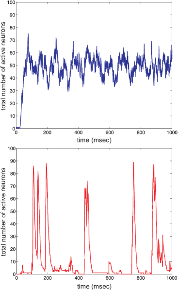
Figure 8: Dynamic evolutions of the net number of active neurons in the neural network example considered in Section VIII-D drawn from the underlying master equation using exact sampling. The blue trajectory indicates that neurons fire asynchronously, whereas, the irregular and isolated bursts of net neural activity observed in the red trajectory indicate that neurons fire synchronously resulting in avalanching.

It has been shown by Benayoun et al. (2010) that when the sum $\nu_{E}+\nu_{I}$ is kept fixed, then the difference $\delta\nu:=\nu_{E}-\nu_{I}$ controls avalanching (see also Fig. 10). More particularly, as $\delta\nu$ increases, the network transitions from asynchronous to synchronous neural firings that lead to avalanching. We illustrate this behavior in Fig. 8, which depicts two trajectories of the net number $A(t)$ of active neurons obtained by sampling the master equation using exact sampling. The blue trajectory has been obtained by setting $\nu_{E}=0.034$ and $\nu_{I}=-0.00062$, whereas, the red trajectory has been obtained by setting $\nu_{E}=0.140$ and $\nu_{I}=-0.136$. Clearly, the blue trajectory indicates that neurons fire asynchronously (in this case, $\delta\nu=0.00276$), whereas, the red trajectory exhibits avalanching with neurons firing synchronously, resulting in irregular and isolated bursts of activity and thus avalanching (in this case, $\delta\nu=0.276$, which is $100$ times larger than the previous value).

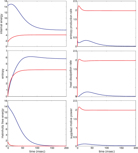
Figure 9: Dynamic evolutions of internal energy, entropy, Helmholtz free energy, entropy production rate, heat dissipation rate, and supplied motive power in the neural network example considered in Section VIII-D for the case of asynchronous (blue lines) and synchronous (red lines) neural firings leading to avalanching.

Most biological systems of interest reach a state of homeostasis, wherein the system is maintained at a given stable operating point. Mathematically, we can describe this point by a stable steady state. From a thermodynamic perspective however such a system must operate away from thermodynamic equilibrium, since living organisms require transfer of energy and mass with their surroundings in order to consume nutrients and excrete waste. To achieve this, nonzero motive power must be supplied to the system at steady-state, which implies that an equal amount must be dissipated to the surroundings in the form of heat, by virtue of the first law of thermodynamics. As a consequence, the state of homeostasis at which biological systems operate is often referred to as the non-equilibrium steady-state (NESS).

Naturally, the neural network discussed in this example must also operate at a NESS [e.g., see Stewart and Plenz (2008)]. Fig. 9 shows clearly that this is indeed the case. This figure depicts the dynamic evolutions of internal energy, entropy, Helmholtz free energy, entropy production rate, heat dissipation rate, and supplied motive power, for the two cases of asynchronous (blue lines) and synchronous neural firings (red lines). Note that all thermodynamic quantities reach stationarity, with the entropy production rate, heat dissipation rate, and supplied motive power converging to the same value in each case, in agreement with the first and second law of thermodynamics. The fact that this value is nonzero in both cases shows that the system operates away from thermodynamic equilibrium at steady-state regardless of the type of neural firings involved.

The results depicted in Fig. 9 show that the system entropy is in general smaller when neurons fire synchronously than when they fire asynchronously. This indicates an expected degree of predictability in neural activity when neurons fire synchronously. On the other hand, the initial Helmholtz free energy associated with asynchronous neural firings is almost an order of magnitude larger than that associated with synchronous firings. In both cases however the Helmholtz free energy becomes zero at steady-state, as expected. This indicates that, under constant temperature and volume, appreciable more work must be done when the neurons fire asynchronously to reach steady-state than when the neurons fire synchronously. It is therefore expected that when neurons fire synchronously, the system will reach steady-state much faster than when neurons fire asynchronously. This is clearly verified by the results depicted in Fig. 9. We may therefore postulate that synchronous neural firing is, among other things, necessary for a neural network to quickly reach a state of homeostasis [see also Stewart and Plenz (2008)].

Fig. 9 also reveals that the stationary value of the supplied motive power (as well as the stationary values of the entropy production and heat dissipation rates) is appreciably larger in the case of synchronous neural firings than asynchronous firings. This difference is well predicted by the theory of dissipative structures Nicolis and Prigogine (1977) according to which self-organization of a system to an ordered internal state requires that the system is sufficiently driven by external sources and dissipates appreciable heat to its surroundings. It is clear from Fig. 9 that appreciable amounts of supplied motive power and heat dissipation is required to achieve avalanching behavior, which leads to an ordered stationary state, quantified by a lower entropy. We may therefore conclude that the emergence of avalanches in a neural network is a consequence of externally driven self-organization accompanied by appreciable heat dissipation. This conclusion is further confirmed by Fig. 10, which depicts the (average) rate of avalanche formation (number of avalanches per unit time, ) the supplied motive power (or heat dissipation), and the system entropy at steady-state. To calculate the number of avalanches present in a given trajectory of net neural activity, we assume that an avalanche occurs within a time window $[t,t+\tau)$ whenever the following three conditions are satisfied: ($i$) $A(t^{\prime})>0$, for all $t^{\prime}\in[t,t+\tau)$; i.e., there is neuronal activity during the time interval $[t,t+\tau)$, ($ii$) there exist some $\epsilon>0$ such that $A(t^{\prime})=0$, for all $t^{\prime}\in[t-\epsilon,t)$; i.e., there is no neural activity immediately before time $t$, and ($iii$) $A(t+\tau)=0$; i.e., there is no neural activity at time $t+\tau$.

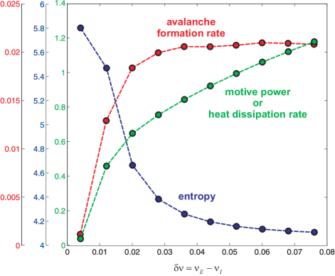
Figure 10: Average rate of avalanche formation (red curve) in the neural network example considered in Section VIII-D (calculated from $1,\!000$ trajectories of net neural activity during a period of $1,\!000$ msec, drawn from the master equation using exact Monte Carlo sampling), supplied motive power (or heat dissipation) at steady-state (green curve), and system entropy at steady-state (blue curve) as a function of the difference $\delta\nu$ between the excitatory and inhibitory weights. As expected, increasing the supply of motive power results in increasing the rate of avalanche formation and decreasing the system entropy.

We conclude by noting that avalanching can be understood at steady-state through the energy landscape $E(\boldsymbol{y})$ [see Eq. (62)]. As a matter of fact, the stationary dynamics of neural activity may be thought of as a random walk on this landscape, where the most likely steps follow a path from higher to lower energy states (i.e., the preference is to move downhill), with occasional (low probability) jumps from lower to higher energy states. In Fig. 11(a), we depict the energy landscape when neurons fire asynchronously, whereas, in Fig. 11(b) we depict the energy landscape when neurons fire synchronously, thus leading to avalanching. One can see that the ground state (global minimum) of the energy landscape depicted in Fig. 11(a) occurs away from the origin at which neural activity is zero. As a consequence, the system spends most time in Gaussian-like fluctuations about the ground state. The system can jump out of the energy well surrounding the ground state and reach the origin, but with very small probability, due to its large width. Therefore, avalanche formation in this system is a rare event. This behavior is in agreement with a recent finding that neural networks may simultaneously support synchronous and asynchronous dynamics, switching between these two modes of operation spontaneously De Ville and Peskin (2008).

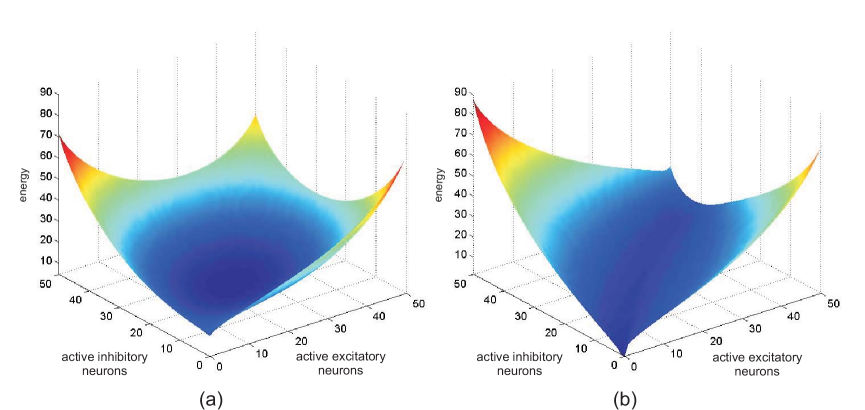
Figure 11: Energy landscape of the neural network example considered in Section VIII-D when: (a) neurons fire asynchronously, and (b) neurons fire synchronously resulting in avalanching.

On the other hand, the energy landscape of the system with synchronous neural firings depicted in Fig. 11(b) contains a valley along the line $Y_{1}=Y_{2}$ of equal excitatory and inhibitory activities, which slopes down to the ground state that is now located at the origin. Thus, from any point on this landscape, the most likely trajectory roles downhill until it reaches the origin. From this point, the dynamics of excitatory and inhibitory neural activities may again reach the valley by randomly jumping away in an uphill motion that overcomes the steep and narrow energy well surrounding the origin. This mechanism results in avalanching, which can be thought of as a random sequence of zero (or almost zero) net neural activity at points in the well surrounding the origin followed by nonzero net neural activity at points proximal to the valley.

IX Outlook

The study of Markov processes on complex reaction networks is an area of research that has been evolving for more than half a century. Its applicability to many scientific and engineering disciplines has led to parallel and often independent developments, which have recently reached a critical mass due to unprecedented advancements in modern experimental procedures and computational capabilities. This can be best illustrated by the sharp increase in the number of articles published on the subject during the last ten years. For this reason, we believe that the present review is both appropriate and timely. Our objective has been to provide a coherent exposure to what has been done so far and illustrate key methods with simple examples. In the following, we conclude this review with a brief discussion of some outstanding issues and problems important to the field. Some old problems require better solutions, whereas, developing novel methods for the analysis of Markovian reaction networks can lead to new and important results. In some cases, the work that needs to be done is at least as challenging and rewarding as the work done so far.

IX.1 Solving the master equation

The tremendous flexibility and generality of Markovian reaction networks make them an excellent mathematical framework for studying stochastic processes on complex networks. The coherency of a single framework means that tools and discoveries made in one field may be readily ported to distant applications. In fact, it has been argued by Cook et al. (2009) that Markovian reaction networks with mass action propensities can perform Turing universal computations with arbitrarily small error, which becomes zero at the thermodynamic limit Magnasco (1997). This strength however turns out to be one of the most profound weaknesses of Markovian reaction networks: there will be no single analytical or even computational method capable of calculating the exact solution of the underlying master equation in complete generality using finite resources. As a consequence, the development of accurate and computationally feasible techniques for studying the dynamic behavior of large nonlinear Markovian reaction networks is still the most important and challenging problem in this field of research.

One way to deal with this problem is to focus on specialized structures that may be present in certain reaction networks and, by exploiting these structures, develop rigorous approximation techniques tailored to the specific application at hand. A good example of such an approach is the IE method discussed in Section IV-B. This method calculates the exact solution of the master equation, up to a desired precision, by exploiting the structure of the master equation that governs the DA process. Moreover, it uses the fact that, in some reaction networks, the sample space associated with the DA process is bounded whereas its cardinality is not appreciably larger than the cardinality of the sample space associated with the population process Jenkinson and Goutsias (2012).

Another possibility is to move away from estimating the joint probability distributions of the DA and population processes and focus on estimating computationally more tractable marginal probability distributions or statistical summaries. Moment closure schemes, in conjunction with MaxEnt methods, seem to be particularly suited in this case. However, much work is needed for developing appropriate closure schemes and evaluating the errors introduced by the resulting approximations, as well as for designing computationally efficient MaxEnt methods. On the other hand, embedding Monte Carlo steps within a computationally efficient method for solving the master equation can prove very useful for guiding correct implementation. For example, employing a second-order moment closure scheme will not be appropriate if a small number of Monte Carlo samples drawn from the master equation reveals a bistable system behavior. The use of hybrid techniques, capable of drawing on relative strengths to mitigate weaknesses of the tools discussed in Sections IV & V, will likely pave the way to more robust solution methodologies, especially for stiff reaction networks. Finally, to deal with the large networks present in many applications, it is necessary to focus on computational efficiency and, in particular, on algorithms that can exploit the highly parallel structure of modern high performance computing platforms.

IX.2 Thermodynamic analysis

Statistical thermodynamics can be effectively used to compactly describe the macroscopic behavior of a given stochastic system by a small number of variables. For this reason, it has been successfully applied in many fields of science and engineering. For example, a container full of gas molecules can be exhaustively described by a set of high-dimensional Hamiltonian equations governing the position and momentum of every single molecule. However, a small number of statistical thermodynamic summaries, such as pressure, temperature, entropy, Helmholtz free energy etc., can be used to provide a more lucid and computationally tractable description of the system. Compact descriptions of system dynamics are also possible in the case of Markovian reaction networks whose analysis, based on statistical thermodynamics, may be the only amenable method of dealing with large nonlinear networks. However, development of such analysis methods are still at their infancy and wide open for future exploration.

A promising line of inquiry seems to be the potential energy landscape perspective discussed in Section VII, which serves as the starting point for developing the thermodynamic analysis tools discussed in Section VIII. Future efforts must focus on designing accurate and efficient methods for estimating the potential energy landscape of Markovian reaction networks and detecting noise-induced modes. The ability to predict noise-induced modes not present as fixed points in the macroscopic equations is an important and challenging task. Since these modes of operation are prominent when appreciable stochastic fluctuations are present and, often, are perched near bifurcation points predicted by the corresponding macroscopic equations Samoilov et al. (2005); Turcotte et al. (2008), it is likely that their study will lead investigators to focus on the interface between stochastic processes and bifurcation theory for nonlinear ODEs.

Aside from the possibility of representing a reaction network using a small number of variables, conditions on the underlying propensity functions imposed by the laws of thermodynamics have shown to be extremely valuable for the modeling and analysis of such networks. For example, the use of thermodynamic constraints can alleviate some burden associated with parameter estimation imposed by the curse of dimensionality and can lead to lower computational complexity, better estimation performance, and reduced data overfitting Colquhoun et al. (2004); Liebermeister and Klipp (2006); Yang et al. (2006); Jenkinson et al. (2010); Jenkinson and Goutsias (2011). Moreover, it can result in physically realizable network models consistent with the fundamental laws of thermodynamics. The work done so far on this important subject has focused on reaction networks with deterministic dynamics. Therefore, extending this line of research to Markovian reaction networks is an exciting prospect with potentially fundamental consequences.

IX.3 Sensitivity analysis

Often, the main focus of analysis of the dynamic behavior of a reaction network is a response function that encapsulates some important system characteristics. In epidemiology, for example, one may not care so much about the specific details of the population dynamics, but would rather focus on the total number of individuals infected by a disease over a given period of time. Another example would be the case of cell signaling, where the detailed interactions of a signaling pathway are not as important as the total amount of a protein produced at the “output” of the pathway. Sensitivity analysis is a quantitative approach designed to investigate how variations in the parameters of a reaction network (e.g., in the specific probability rate constants associated with the propensity functions of a mass action system) affect a response function of interest Heinrich and Schuster (1996); Varma et al. (1999); Saltelli et al. (2005, 2008).

Many physical and man-made reaction networks are designed to be robust to random fluctuations (or even failures) in system components. Although robustness is a highly desirable property, it results in a small number of parameters having a disproportionately large influence on the system response. As a consequence, a robust reaction network can be quite vulnerable to targeted attacks on influential components, which can be a blessing or a curse, depending on the particular situation at hand. For example, development of new drugs may greatly benefit from this property since, to reduce or even eliminate the effects of a disease caused by deregulation of key system responses, it may be sufficient to design a drug that only inhibits influential reactions that shape these responses. On the other hand, targeted attacks on national infrastructure by hackers or terrorists may produce large scale disruptions with devastating results.

The objective of sensitivity analysis is to determine those factors in a reaction network that produce no noticeable variations in system response and identify those factors that are most influential in shaping that response. Although this is a powerful analysis technique with important practical consequences, it comes with a large computational cost, even in the case of reaction networks with deterministic dynamics Zhang et al. (2009); Zhang and Goutsias (2010, 2011). For this reason, the development of practical methods for sensitivity analysis of Markovian reaction networks is still at their infancy Gunawan et al. (2005); Kim et al. (2007); Plyasunov and Arkin (2007); Dandach and Khammash (2010); Kim and Sauro (2010); Rathinam et al. (2010); Komorowski et al. (2011); Warren and Allen (2012).

In the stochastic context, sensitivity analysis involves computing the solution of the master equation using different parameter values. As a consequence, the development of efficient solution methods that can be implemented on parallel computer architectures, paired with novel sensitivity estimators, will ensure the feasibility of this type of analysis. We should also note that it has been recently demonstrated by Zhang et al. (2009) and Zhang and Goutsias (2011) that, at least for the case of physical reaction networks with deterministic dynamics, sensitivity analysis methods must be in agreement with underlying thermodynamic constraints. As a consequence, developing accurate, computationally efficient, and thermodynamically consistent sensitivity analysis methods for Markovian reaction networks is an important research activity with significant benefits.

IX.4 Statistical inference

In general, there are two fundamentally different types of parameters associated with a Markovian reaction network model: the stoichiometric coefficients $\nu_{nm}$ and $\nu^{\prime}_{nm}$ that determine the structure of the network, and the kinetic parameters that determine the non-structural portion of the propensity functions. Some parameter values can be deduced experimentally or by means of appropriate theoretical and sometimes heuristic arguments. Most parameters however must be estimated from available data using statistical inference techniques. Since the predictive power of a given model is fundamentally constrained by the accuracy of its parameterization, inferring the unknown parameter values in a Markovian reaction network is a problem of paramount interest and practical importance. Although this problem has been extensively studied for reaction networks with deterministic dynamics Moles et al. (2003); Crampin et al. (2004); Maria (2004), the statistical inference of Markovian reaction networks is largely an open research problem. This problem has been recently investigated by Golightly and Wilkinson (2005, 2006), Reinker et al. (2006), Boys et al. (2008), Komorowski et al. (2009), Poovathingal and Gunawan (2010), Wang et al. (2010d), and Daigle Jr. et al. (2012), but the resulting algorithms do not adequately address important issues, such as curse of dimensionality, thermodynamic consistency, and computational efficiency. These methods have been primarily designed for biochemical reaction networks, but can be easily adopted in other applications with little or no effort.

In most approaches to statistical inference, it is quite common to assume known structural parameters and proceed with estimating the kinetic parameters using noisy and sparse measurements of system dynamics. This problem, known as model calibration, is much easier than the problem of estimating the structural parameters, which is often referred to as model selection.

The two most difficult issues associated with model calibration is the curse of dimensionality and the use of non-convex cost functions which complicate numerical optimization. Curse of dimensionality refers to a very fast growth of the volume of the parameter space in terms of the number of unknown parameters to be estimated. As a consequence, the problem of finding the “best” parameter values becomes increasingly difficult as the number of unknown parameters increases. This is further exacerbated by the non-convex optimization problem of finding these values, which is computationally very difficult to solve in most cases of interest Spall (2003). Therefore, the development of statistical techniques for accurate and computationally efficient model calibration of Markovian reaction networks is a very challenging problem. Possible ways to attack this problem is to effectively reduce the number of parameters that must be estimated by incorporating appropriate constraints [e.g., constraints imposed by the fundamental laws of thermodynamics Colquhoun et al. (2004); Liebermeister and Klipp (2006); Yang et al. (2006); Jenkinson et al. (2010); Jenkinson and Goutsias (2011)] and to identify a smaller set of “influential” parameters whose values must be estimated with sufficient precision [e.g., by employing a sensitivity analysis approach Jenkinson et al. (2010)]. This reduction in dimensionality must be combined with fast algorithms for solving the master equation, with efficient optimization methods, and appropriately designed experimental protocols for collecting data with high information content about the values of the unknown parameters Jenkinson and Goutsias (2010).

In general, model selection is a more difficult problem. Solving this problem will require the development of novel hypothesis testing approaches for comparing between two competing network models (e.g., an originally proposed signaling network and another network obtained by adding new reactions) in a rigorous statistical fashion. This approach however requires that both models are calibrated before compared to each other (e.g., by a likelihood ratio test), which substantially adds to the difficulty of the problem. Another major issue is that more complex models are expected to be more capable of closely matching experimental data, but these models may result in undesirable overfitting. It is therefore necessary to develop methods that appropriately penalize model complexity so that the chosen “optimal” model is the most parsimonious model capable of adequately explaining available data. Finally, all of this must be done while taking into account possible constraints imposed on the structural and kinetic parameters of the network (e.g., by prior knowledge on feasible structural parameter values and by the fundamental laws of thermodynamics).

IX.5 Adaptive Markovian reaction networks

An important aspect of many real-life interaction networks is that the network topology, quantified by the stoichiometric coefficients $\nu_{nm}$ and $\nu^{\prime}_{nm}$, is intricately coupled with the network dynamics. As we mentioned in Section II-B-3, for all reaction networks encountered in practice, the propensity functions depend on the stoichiometric coefficients $\nu_{nm}$ and, therefore, the topological structure of a reaction network directly affects its dynamics. However, the opposite is also true: the dynamics can influence the underlying network topology. In opinion formation, for example, individuals form their beliefs based on interactions determined by the underlined social network, whereas, individuals with similar beliefs tend to eventually influence each other. In these cases, modeling dynamics on complex networks by assuming fixed topology is legitimate only when the time scale of interest is sufficiently smaller than the time scale of change in network topology.

Recently, several articles have appeared in the literature introducing adaptive networks that take into account the interplay between network topology and dynamics Ehrhardt et al. (2006); Gross et al. (2006); Holme and Newman (2006); Zhou and Kurths (2006); Gross and Blasius (2008); Ren et al. (2010); Zhang et al. (2010b); Yuan and Zhou (2011). These preliminary works clearly demonstrate that a number of intriguing properties emerge, not previously observed in nonadaptive networks: formation of complex topologies, spontaneous emergence of modular organization, more complex dynamics than the ones observed in nonadaptive models, and self-organization towards a highly robust critical behavior characterized by power-law distributions.

Understanding the coupling between Markovian dynamics and network topology is a fascinating subject of research that can eventually lead to surprising new theoretical results and novel computational methods for the modeling and analysis of networks with significant impact in many fields. For example, adaptive Markovian reaction networks may potentially lead to a better understanding of how cell biology at the molecular level has evolved towards certain types of reaction network architectures and motifs, characterized by a high degree of modularity and robustness. These type of networks can be represented by master equations with time-dependent stoichiometric coefficients, whose values are updated by the system state following well-defined rules. We foresee a rapid growth in developing such models that can lead to many fascinating and novel results to come.

X Conclusion

The recent burst in the amount of research efforts for studying random processes on complex interaction networks has been driven primarily by impressive advances in experimental techniques for measuring these processes and by a clear understanding that stochasticity plays a fundamental role in shaping the transient and steady-state dynamic behavior of real-life networks. This effort has reinforced the fact that the theory of Markovian reaction networks is at the foundation of most modeling and analysis techniques for studying stochastic dynamical systems on networks with applications in diverse fields, such as chemistry, biology, sociology, epidemiology, pharmacology, theoretical neuroscience, and engineering. The main goal of this review was to summarize, in a systematic fashion, what is known so far about this exciting field and briefly discuss some open problems that need to be solved and new methodologies that must be developed. We believe that a major effort should be focused on introducing new concepts and ideas that might lead to novel and practical tools for the modeling and analysis of stochastic dynamics on interaction networks encountered in practice. We hope that this article will be used as a reference by network scientists across different scientific disciplines and help to catalyze exciting new developments in these fields.

References

- Abou-Kandil et al. (2003) Abou-Kandil, H., G. Freiling, V. Ionescu, and G. Jank, 2003, Matrix Riccati Equations in Control and Systems Theory (Birkhäuser Verlag, Basel, Switzerland).
- Abramov (2010) Abramov, R. V., 2010, Commun. Math. Sci. 8(2), 377.
- Aldous (1982) Aldous, D. J., 1982, Stoch. Proc. Appl. 13, 305.
- Anderson (2007) Anderson, D. F., 2007, J. Chem. Phys. 127, 214107.
- Anderson (2008) Anderson, D. F., 2008, J. Chem. Phys. 128, 054103.
- Andrieux and Gaspard (2004) Andrieux, D., and P. Gaspard, 2004, J. Chem. Phys. 121(13), 6167.
- Andrieux and Gaspard (2007) Andrieux, D., and P. Gaspard, 2007, J. Stat. Phys. 127(1), 107.
- Antal et al. (2006) Antal, T., P. L. Krapivsky, and S. Redner, 2006, Physica D 224, 130.
- Ao (2004) Ao, P., 2004, J. Phys. A: Math. Gen. 37, L25.
- Ao et al. (2007) Ao, P., C. Kwon, and H. Qian, 2007, Complexity 12(4), 19.
- Artyomov et al. (2007) Artyomov, M. N., J. Das, M. Kardar, and A. K. Chakraborty, 2007, Proc. Natl. Acad. Sci. USA 104(48), 18958.
- Artyomov et al. (2009) Artyomov, M. N., M. Mathur, M. S. Samoilov, and A. K. Chakraborty, 2009, J. Chem. Phys. 131, 195103.
- Auger et al. (2009) Auger, P., R. Mchich, T. Chowdhury, G. Sallet, M. Tchuente, and J. Chattopadhyay, 2009, J. Theor. Biol. 258(3), 344.
- Bailey (1950) Bailey, N. T. J., 1950, Biometrika 37(3–4), 193.
- Bailey (1957) Bailey, N. T. J., 1957, The Mathematical Theory of Epidemics (Griffin, London).
- Bailey (1963) Bailey, N. T. J., 1963, Biometrika 50(3–4), 235.
- Ball et al. (2006) Ball, K., T. G. Kurtz, L. Popovic, and G. Rempala, 2006, Ann. Appl. Probab. 16(4), 1925.
- Bandyopadhyay et al. (2005) Bandyopadhyay, K., A. K. Bhattacharya, P. Biswas, and D. A. Drabold, 2005, Phys. Rev. E 71, 057701.
- Barabási and Oltvai (2004) Barabási, A.-L., and Z. N. Oltvai, 2004, Nat. Rev. Genet. 5(2), 101.
- Bartholomay (1958) Bartholomay, A. F., 1958, Bull. Math. Biophys. 20, 175.
- Bartholomay (1959) Bartholomay, A. F., 1959, Bull. Math. Biophys. 21, 363.
- Bartholomay (1962) Bartholomay, A. F., 1962, Biochemistry 1(2), 223.
- Bartlett (1949) Bartlett, M. S., 1949, J. Roy. Statist. Soc. B 11(2), 211.
- Bartlett (1957) Bartlett, M. S., 1957, J. Roy. Statist. Soc. A 120, 48.
- Bartlett (1960) Bartlett, M. S., 1960, Stochastic Population Models in Ecology and Epidemiology (Methuen, London).
- Bascompte (2009) Bascompte, J., 2009, Science 325, 416.
- Bascompte (2010) Bascompte, J., 2010, Science 329, 765.
- Ben-Zion et al. (2010) Ben-Zion, Y., Y. Cohen, and N. M. Shnerb, 2010, J. Theor. Biol. 264, 197.
- Benayoun et al. (2010) Benayoun, M., J. D. Cowan, W. van Drongelen, and E. Wallace, 2010, PLoS Comput. Biol. 6(7), e1000846.
- Bishop and Qian (2010) Bishop, L. M., and H. Qian, 2010, Biophys. J. 98, 1.
- Black and McKane (2010) Black, A. J., and A. J. McKane, 2010, J. R. Soc. Interface 7(49), 1219.
- Black and McKane (2012) Black, A. J., and A. J. McKane, 2012, Trends Ecol. Evol. 27(6), 337.
- Blake et al. (2003) Blake, W. J., M. Kaern, C. R. Cantor, and J. J. Collins, 2003, Nature 422, 633.
- Bois et al. (1990) Bois, F. Y., L. Zeise, and T. N. Tozer, 1990, Toxicol. Appl. Pharm. 102, 300.
- Borgatti et al. (2009) Borgatti, S. P., A. Mehra, D. J. Brass, and G. Labianca, 2009, Science 323, 892.
- Bostani et al. (2012) Bostani, N., D. A. Kessler, N. M. Shnerb, W.-J. Rappel, and H. Levine, 2012, Phys. Rev. E 85, 011901.
- Boys et al. (2008) Boys, R. J., D. J. Wilkinson, and T. B. L. Kirkwood, 2008, Stat. Comput. 18, 125.
- Bressloff (2009) Bressloff, P. C., 2009, SIAM J. Appl. Math. 70(5), 1488.
- Bressloff (2010) Bressloff, P. C., 2010, Phys. Rev. E 82, 051903.
- van den Broeck and Esposito (2010) van den Broeck, C., and M. Esposito, 2010, Phys. Rev. E 82, 011144.
- Buice and Cowan (2007) Buice, M. A., and J. D. Cowan, 2007, Phys. Rev. E 75, 051919.
- Buice et al. (2010) Buice, M. A., J. D. Cowan, and C. C. Chow, 2010, Neural Comput. 22, 377.
- Cai (2007) Cai, X., 2007, J. Chem. Phys. 126, 124108.
- Cai and Wen (2009) Cai, X., and J. Wen, 2009, J. Chem. Phys. 131, 064108.
- Cai and Xu (2007) Cai, X., and Z. Xu, 2007, J. Chem. Phys. 126, 074102.
- Cao et al. (2005a) Cao, Y., D. T. Gillespie, and L. R. Petzold, 2005a, J. Chem. Phys. 123, 054104.
- Cao et al. (2005b) Cao, Y., D. T. Gillespie, and L. R. Petzold, 2005b, J. Chem. Phys. 122, 014116.
- Cao et al. (2006) Cao, Y., D. T. Gillespie, and L. R. Petzold, 2006, J. Chem. Phys. 124, 044109.
- Cao et al. (2007) Cao, Y., D. T. Gillespie, and L. R. Petzold, 2007, J. Chem. Phys. 126, 224101.
- Cao et al. (2004) Cao, Y., H. Li, and L. R. Petzold, 2004, J. Chem. Phys. 121(9), 4059.
- Chaouiya (2007) Chaouiya, C., 2007, Brief. Bioinform. 8(4), 210.
- Chatterjee et al. (2005a) Chatterjee, A., K. Mayawala, J. S. Edwards, and D. G. Vlachos, 2005a, Boinformatics 21(9), 2136.
- Chatterjee et al. (2005b) Chatterjee, A., D. G. Vlachos, and M. A. Katsoulakis, 2005b, J. Chem. Phys. 122, 024112.
- Chen and Bokka (2005) Chen, W. Y., and S. Bokka, 2005, J. Theor. Biol. 234, 455.
- Chevalier and El-Samad (2009) Chevalier, M. W., and H. El-Samad, 2009, J. Chem. Phys. 131, 054102.
- Chevalier and El-Samad (2011) Chevalier, M. W., and H. El-Samad, 2011, J. Chem. Phys. 135, 214110.
- Cohn and Kumar (2009) Cohn, H., and A. Kumar, 2009, Proc. Natl. Acad. Sci. USA 106(24), 9570.
- Colquhoun et al. (2004) Colquhoun, D., K. A. Dowsland, M. Beato, and A. J. Plested, 2004, Biophys. J. 86, 3510.
- Cook et al. (2009) Cook, M., D. Soloveichik, E. Winfree, and J. Bruck, 2009, in Algorithmic Bioprocesses, edited by A. Condon, D. Harel, J. N. Kok, A. Salomaa, and E. Winfree (Springer-Verlag, Berlin), Natural Computing Series, pp. 543–584.
- Cotter et al. (2011) Cotter, S. L., K. C. Zygalakis, I. G. Kevrekidis, and R. Erban, 2011, J. Chem. Phys. 135, 094102.
- Cover and Thomas (1991) Cover, T. M., and J. A. Thomas, 1991, Elements of Information Theory (John Wiley & Sons, New York).
- Cowan (1991) Cowan, J. D., 1991, in Advances in Neural Information Processing Systems, edited by R. P. Lippman, J. E. Moody, and D. S. Touretzky (Morgan Kaufmann, San Mateo, CA), volume 3, pp. 62–69.
- Crampin et al. (2004) Crampin, E. J., S. Schnell, and P. E. McSharry, 2004, Prog. Biophys. Mol. Bio. 86, 77.
- Crudu et al. (2009) Crudu, A., A. Debussche, and O. Radulescu, 2009, BMC Syst. Biol. 3, 89.
- Daigle Jr. et al. (2011) Daigle Jr., B. J., M. K. Roh, D. T. Gillespie, and L. R. Petzold, 2011, J. Chem. Phys. 134, 044110.
- Daigle Jr. et al. (2012) Daigle Jr., B. J., M. K. Roh, L. R. Petzold, and J. Niemi, 2012, BMC Bioinf. 13, 68.
- Dandach and Khammash (2010) Dandach, S. H., and M. Khammash, 2010, PLoS Comput. Biol. 6(11), e1000985.
- Darvey and Staff (1966) Darvey, I. G., and P. J. Staff, 1966, J. Chem. Phys. 44(3), 990.
- Datta et al. (2010) Datta, S., G. W. Delius, and R. Law, 2010, B. Math. Biol. 72, 1361.
- De Ville and Peskin (2008) De Ville, R. E. L., and C. S. Peskin, 2008, Bull. Math. Biol. 70, 1608.
- Delbrück (1940) Delbrück, M., 1940, J. Chem. Phys. 8, 120.
- Demirel (2010) Demirel, Y., 2010, J. Non-Newtonian Fluid Mech. 165, 953.
- Deuflhard et al. (2008) Deuflhard, P., W. Huisinga, T. Jahnke, and M. Wulkow, 2008, SIAM J. Sci. Comput. 30(6), 2990.
- Diaz (2009) Diaz, M., 2009, Petri Nets: Fundamental Models, Verification and Applications (Wiley-ISTE, Hoboken, New Jersey).
- Diestel (1997) Diestel, R., 1997, Graph Theory (Springer, New York).
- Dilão and Domingos (2000) Dilão, R., and T. Domingos, 2000, Ecol. Model. 132, 191.
- Dill and Bromberg (2011) Dill, K. A., and S. Bromberg, 2011, Molecular Driving Forces: Statistical Thermodynamics in Biology, Chemistry, Physics, and Nanoscience (Galand Science, New York), 2nd edition.
- E et al. (2005) E, W., D. Liu, and E. Vanden-Eijnden, 2005, J. Chem. Phys. 123, 194107.
- E et al. (2007) E, W., D. Liu, and E. Vanden-Eijnden, 2007, J. Comput. Phys. 221, 158.
- Ehrhardt et al. (2006) Ehrhardt, G. C. M. A., M. Marsili, and F. Vega-Redondo, 2006, Phys. Rev. E 74, 036106.
- El Boustani and Destexhe (2009) El Boustani, S., and A. Destexhe, 2009, Neural Comput. 21, 46.
- Elf and Ehrenberg (2003) Elf, J., and M. Ehrenberg, 2003, Genome Res. 13, 2475.
- Elowitz et al. (2002) Elowitz, M. B., A. J. Levine, E. D. Siggia, and P. S. Swain, 2002, Science 297, 1183.
- Engblom (2006) Engblom, S., 2006, Appl. Math. Comput. 180, 498.
- Esposito and van den Broeck (2010a) Esposito, M., and C. van den Broeck, 2010a, Phys. Rev. Lett. 104, 090601.
- Esposito and van den Broeck (2010b) Esposito, M., and C. van den Broeck, 2010b, Phys. Rev. E 82, 011143.
- Ferm et al. (2008) Ferm, L., P. Lötstedt, and A. Hellander, 2008, J. Sci. Comput. 34, 127.
- Freeman (2004) Freeman, L. C., 2004, The Development of Social Network Analysis: A Study in the Sociology of Science (Emprirical Press, Vancouver).
- Gadgil et al. (2005) Gadgil, C., C. H. Lee, and H. G. Othmer, 2005, B. Math. Biol. 67, 901.
- Gardiner (2010) Gardiner, C., 2010, Stochastic Methods: A Handbook for the Natural and Social Sciences (Springer, Berlin), 4th edition.
- Gaspard (2004) Gaspard, P., 2004, J. Chem. Phys. 120(19), 8898.
- Ge (2009) Ge, H., 2009, Phys. Rev. E 80, 021137.
- Ge and Qian (2010) Ge, H., and H. Qian, 2010, Phys. Rev. E 81, 051133.
- Ge et al. (2012) Ge, H., H. Qian, and M. Qian, 2012, Phys. Rep. 510, 87.
- Gibson and Bruck (2000) Gibson, M. A., and J. Bruck, 2000, J. Phys. Chem. A 104, 1876.
- Gillespie (2009) Gillespie, C. S., 2009, IET Syst. Biol. 3(1), 52.
- Gillespie (1976) Gillespie, D. T., 1976, J. Comput. Phys. 22, 403.
- Gillespie (1977) Gillespie, D. T., 1977, J. Phys. Chem. 81(25), 2340.
- Gillespie (1992) Gillespie, D. T., 1992, Physica A 188, 404.
- Gillespie (1996) Gillespie, D. T., 1996, Am. J. Phys. 64(10), 1246.
- Gillespie (2000) Gillespie, D. T., 2000, J. Chem. Phys. 113(1), 297.
- Gillespie (2001) Gillespie, D. T., 2001, J. Chem. Phys. 115(4), 1716.
- Gillespie and Petzold (2003) Gillespie, D. T., and L. R. Petzold, 2003, J. Chem. Phys. 119(16), 8229.
- Gillespie et al. (2009) Gillespie, D. T., M. Roh, and L. R. Petzold, 2009, J. Chem. Phys. 130, 174103.
- Golightly and Wilkinson (2005) Golightly, A., and D. J. Wilkinson, 2005, Biometrics 61, 781.
- Golightly and Wilkinson (2006) Golightly, A., and D. J. Wilkinson, 2006, J. Comput. Biol. 13(3), 838.
- Gómez-Uribe and Verghese (2007) Gómez-Uribe, C. A., and G. C. Verghese, 2007, J. Chem. Phys. 126, 024109.
- Gómez-Uribe et al. (2008) Gómez-Uribe, C. A., G. C. Verghese, and A. R. Tzafiri, 2008, J. Chem. Phys. 129, 244112.
- Goss and Peccoud (1998) Goss, P. J. E., and J. Peccoud, 1998, Proc. Natl. Acad. Sci. USA 95, 6750.
- Goutsias (2005) Goutsias, J., 2005, J. Chem. Phys. 122, 184102.
- Goutsias (2006) Goutsias, J., 2006, IEEE/ACM Trans. Comput. Biol. Boinf. 3(1), 57.
- Goutsias (2007) Goutsias, J., 2007, Biophys. J. 92, 2350.
- Grima (2010) Grima, R., 2010, J. Chem. Phys. 133, 035101.
- Grima (2011) Grima, R., 2011, Phys. Rev. E 84, 056109.
- Grima (2012) Grima, R., 2012, J. Chem. Phys. 136, 154105.
- Grima et al. (2011) Grima, R., P. Thomas, and A. V. Straube, 2011, J. Chem. Phys. 135, 084103.
- Gross and Blasius (2008) Gross, T., and B. Blasius, 2008, J. R. Soc. Interface 5, 259.
- Gross et al. (2006) Gross, T., C. J. D. D’Lima, and B. Blasius, 2006, Phys. Rev. Lett. 96, 208701.
- Gunawan et al. (2005) Gunawan, R., Y. Cao, L. Petzold, and F. J. Doyle III, 2005, Biophys. J. 88, 2530.
- Haas (2002) Haas, P. J., 2002, Stochastic Petri Nets: Modeling, Stability, Simulation (Springer-Verlag, New York).
- Haken (1974) Haken, H., 1974, Phys. Lett. A 46, 443.
- Haken (1975) Haken, H., 1975, Rev. Mod. Phys. 47(1), 67.
- Han and Wang (2007) Han, B., and J. Wang, 2007, Biophys. J. 92, 3755.
- Han and Wang (2008) Han, B., and J. Wang, 2008, Phys. Rev. E 77, 031922.
- Hänggi and Talkner (1980) Hänggi, P., and P. Talkner, 1980, J. Stat. Phys. 22(1), 65.
- Hardman and Limbird (2001) Hardman, J. G., and L. E. Limbird, 2001, Goodman & Gilman’s The Pharmacological Basis of Therapeutics (Mc Graw-Hill, New York), 10th edition.
- Harris and Clancy (2006) Harris, L. A., and P. Clancy, 2006, J. Chem. Phys. 125, 144107.
- Harris et al. (2009) Harris, L. A., A. M. Piccirilli, E. R. Majusiak, and P. Clancy, 2009, Phys. Rev. E 79, 051906.
- Haseltine and Rawlings (2002) Haseltine, E. L., and J. B. Rawlings, 2002, J. Chem. Phys. 117(15), 6959.
- Haseltine and Rawlings (2005) Haseltine, E. L., and J. B. Rawlings, 2005, J. Chem. Phys. 123, 164115.
- Haskey (1954) Haskey, H. W., 1954, Biometrika 41, 272.
- Hasty et al. (2000) Hasty, J., J. Pradines, M. Dolnik, and J. J. Collins, 2000, Proc. Natl. Acad. Sci. USA 97(5), 2075.
- Hayot and Jayaprakash (2004) Hayot, F., and C. Jayaprakash, 2004, Phys. Biol. 1, 205.
- Hegland et al. (2007) Hegland, M., C. Burden, L. Santoso, S. MacNamara, and H. Booth, 2007, J. Comput. Appl. Math. 205, 708.
- Hegland et al. (2008) Hegland, M., A. Hellander, and P. Lötstedt, 2008, BIT 48, 265.
- Heiner et al. (2008) Heiner, M., D. Gilbert, and R. Donaldson, 2008, in Formal Methods for Computational Systems Biology, edited by M. Bernardo, P. Degano, and G. Zavattaro (Springer-Verlag, Berlin), volume 5016 of Lecture Notes in Computer Science, pp. 215–264.
- Heinrich and Schuster (1996) Heinrich, R., and S. Schuster, 1996, The Regulation of Cellular Systems (Chapman & Hall, New York).
- Hellander (2008) Hellander, A., 2008, J. Chem. Phys. 128, 154109.
- Hellander and Lötstedt (2007) Hellander, A., and P. Lötstedt, 2007, J. Comput. Phys. 227, 100.
- Hethcote (2000) Hethcote, H. W., 2000, SIAM Rev. 42(4), 599.
- Heuett and Qian (2006) Heuett, W. J., and H. Qian, 2006, J. Chem. Phys. 124, 044110.
- Hiebeler (2006) Hiebeler, D., 2006, Bull. Math. Biol. 68, 1315.
- Higham (2001) Higham, D. J., 2001, SIAM Rev. 43(3), 525.
- Hill et al. (2010) Hill, A. L., D. G. Rand, M. A. Nowak, and N. A. Christakis, 2010, PLoS Comput. Biol. 6(11), e1000968.
- Hill and Severo (1969) Hill, R. T., and N. C. Severo, 1969, Biometrika 56(1), 183.
- Holme and Newman (2006) Holme, P., and M. E. J. Newman, 2006, Phys. Rev. E 74, 056108.
- Ishida (1958) Ishida, K., 1958, Bull. Chem. Soc. Japan 33, 1030.
- Ishida (1964) Ishida, K., 1964, J. Chem. Phys. 41(8), 2472.
- Isserlis (1918) Isserlis, L., 1918, Biometrika 12(1/2), 134.
- Jahnke (2010) Jahnke, T., 2010, SIAM J. Sci. Comput. 31(6), 4373.
- Jahnke and Huisinga (2007) Jahnke, T., and W. Huisinga, 2007, J. Math. Biol. 54, 1.
- Jahnke and Huisinga (2008) Jahnke, T., and W. Huisinga, 2008, Bull. Math. Biol. 70, 2283.
- Jahnke and Udrescu (2010) Jahnke, T., and T. Udrescu, 2010, J. Comput. Phys. 229, 5724.
- Jenkinson and Goutsias (2011) Jenkinson, G., and J. Goutsias, 2011, BMC Syst. Biol. 5, 64.
- Jenkinson and Goutsias (2012) Jenkinson, G., and J. Goutsias, 2012, PLoS One 7(5), e36160.
- Jenkinson et al. (2010) Jenkinson, G., X. Zhong, and J. Goutsias, 2010, BMC Bioinf. 11, 547.
- Jenkinson and Goutsias (2010) Jenkinson, W. G., and J. Goutsias, 2010, in Proceedings of the 2010 IEEE International Workshop on Genomic Signal Processing and Statistics (Cold Spring Harbor Laboratory, New York), pp. 214–219.
- Jiang et al. (2004) Jiang, D.-Q., M. Qian, and M.-P. Qian, 2004, Mathematical Theory of Nonequilibrium Steady States, volume 1833 of Lecture Notes in Mathematics (Springer-Verlag, Berlin).
- van Kampen (1961) van Kampen, N. G., 1961, Can. J. Phys. 39, 551.
- van Kampen (1973) van Kampen, N. G., 1973, Biometrika 60(2), 419.
- van Kampen (1976) van Kampen, N. G., 1976, in Advance in Chemical Physics, edited by I. Prigogine and S. A. Rice (John Wiley & Sons, New York), volume 34, pp. 245–309.
- van Kampen (2007) van Kampen, N. G., 2007, Stochastic Processes in Physics and Chemistry (Elsevier, Amsterdam), 3rd edition.
- Kang and Kurtz (2012) Kang, H.-W., and T. G. Kurtz, 2012, Ann. Appl. Probab. (To Appear), 1.
- Kapur (1990) Kapur, J. N., 1990, Maximum-entropy Models in Science and Engineering (Wiley, New York).
- Keeling (2000) Keeling, M. J., 2000, J. Theor. Biol. 205, 269.
- Keeling and Ross (2008) Keeling, M. J., and J. V. Ross, 2008, J. R. Soc. Interface 5, 171.
- Keeling and Ross (2009) Keeling, M. J., and J. V. Ross, 2009, Theor. Popul. Biol. 75, 133.
- Keizer (1987) Keizer, J., 1987, Statistical Thermodynamics of Nonequilibrium Processes (Springer-Verlag, New York).
- Kepler and Elston (2001) Kepler, T. B., and T. C. Elston, 2001, Biophys. J. 81, 3116.
- Kim et al. (2007) Kim, D., B. J. Debusschere, and H. N. Najm, 2007, Biophys. J. 92, 379.
- Kim and Sauro (2010) Kim, K. H., and H. M. Sauro, 2010, Math. Biosci. 226, 109.
- Kim and Wang (2007) Kim, K.-Y., and J. Wang, 2007, PLoS Comput. Biol. 3(3), e60.
- Kiss and Simon (2012) Kiss, I. Z., and P. L. Simon, 2012, Bull. Math. Biol. 74(7), 1501.
- Klamt et al. (2009) Klamt, S., U.-U. Haus, and F. Theis, 2009, PLoS Comput. Biol. 5(5), e1000385.
- Komorowski et al. (2011) Komorowski, M., M. J. Costa, D. A. Rand, and M. P. H. Stumpf, 2011, Proc. Natl. Acad. Sci. USA 108(21), 8645.
- Komorowski et al. (2009) Komorowski, M., B. Finkenstädt, C. V. Harper, and D. A. Rand, 2009, BMC Bioinf. 10, 343.
- Krishnarajah et al. (2005) Krishnarajah, I., A. Cook, G. Marion, and G. Gibson, 2005, B. Math. Biol. 67, 855.
- Krishnarajan et al. (2007) Krishnarajan, I., G. Marion, and G. Gibson, 2007, Math. Biosci. 208, 621.
- Kurtz (1971) Kurtz, T. G., 1971, J. Appl. Prob. 8, 344.
- Kurtz (1972) Kurtz, T. G., 1972, J. Chem. Phys. 57(7), 2976.
- Kurtz (1980) Kurtz, T. G., 1980, Ann. Probab. 8(4), 682.
- Kuwahara and Mura (2008) Kuwahara, H., and I. Mura, 2008, J. Chem. Phys. 129, 165101.
- Lafuerza and Toral (2010) Lafuerza, L. F., and R. Toral, 2010, J. Stat. Phys. 140, 917.
- de la Lama et al. (2006) de la Lama, M. S., I. G. Szendro, J. R. Iglesias, and H. S. Wio, 2006, Eur. Phys. J. B 51, 435.
- Lapidus et al. (2008) Lapidus, S., B. Han, and J. Wang, 2008, Proc. Natl. Acad. Sci. USA 105(16), 6039.
- Lässig et al. (2001) Lässig, M., U. Bastolla, S. C. Manrubia, and A. Valleriani, 2001, Phys. Rev. Lett. 86(19), 4418.
- Laurenzi (2000) Laurenzi, I. J., 2000, J. Chem. Phys. 113(8), 3315.
- Lee et al. (2009) Lee, C.-H., K.-H. Kim, and P. Kim, 2009, J. Chem. Phys. 130, 134107.
- Leonard and Reichl (1990) Leonard, D., and L. E. Reichl, 1990, J. Chem. Phys. 92(10), 6004.
- Li et al. (2011) Li, C., E. Wang, and J. Wang, 2011, PLoS One 6(3), e17888.
- Liebermeister and Klipp (2006) Liebermeister, W., and E. Klipp, 2006, Theor. Biol. Med. Model. 3, 41.
- Lipshtat (2007) Lipshtat, A., 2007, J. Chem. Phys. 126, 184103.
- Liu (2001) Liu, J. S., 2001, Monte Carlo Strategies in Scientific Computing (Springer-Verlag, New York).
- Lu et al. (2004) Lu, T., D. Volfson, L. Tsimring, and J. Hasty, 2004, Syst. Biol. 1(1), 121.
- Luo et al. (2002) Luo, J., N. Zhao, and B. Hu, 2002, Phys. Chem. Chem. Phys. 4, 4149.
- Macheras and Iliadis (2006) Macheras, P., and A. Iliadis, 2006, Modeling in Biopharmaceutics, Pharmacokinetics, and Pharmacodynamics (Springer, New York).
- MacNamara et al. (2008) MacNamara, S., K. Burrage, and R. B. Sidje, 2008, Multiscale Model. Simul. 6(4), 1146.
- Magnasco (1997) Magnasco, M. O., 1997, Phys. Rev. Lett. 78(6), 1190.
- Mansour et al. (1981) Mansour, M. M., C. van Den Broeck, G. Nicolis, and J. W. Turner, 1981, Ann. Phys. 131, 283.
- Maria (2004) Maria, G., 2004, Chem. Biochem. Eng. Q. 18(3), 195.
- Mastny et al. (2007) Mastny, E. A., E. L. Haseltine, and J. B. Rawlings, 2007, J. Chem. Phys. 127, 094106.
- Masuda et al. (2010) Masuda, N., N. Gibert, and S. Redner, 2010, Phys. Rev. E 82, 010103.
- Matis and Kiffe (1999) Matis, J. H., and T. R. Kiffe, 1999, Theor. Popul. Biol. 56, 139.
- Matis and Kiffe (2002) Matis, J. H., and T. R. Kiffe, 2002, Environ. Ecol. Stat. 9, 237.
- McAdams and Arkin (1997) McAdams, H. H., and A. Arkin, 1997, Proc. Natl. Acad. Sci. USA 94, 814.
- McCollum et al. (2006) McCollum, J. M., G. D. Peterson, C. D. Cox, M. L. Simpson, and N. F. Samatova, 2006, Comput. Biol. Chem. 30(1), 39.
- McQuarrie (1963) McQuarrie, D. A., 1963, J. Chem. Phys. 38(2), 433.
- McQuarrie (1967) McQuarrie, D. A., 1967, J. Appl. Prob. 4, 413.
- McQuarrie et al. (1964) McQuarrie, D. A., C. J. Jachimowski, and M. E. Russell, 1964, J. Chem. Phys. 40(10), 2914.
- Mead and Papanicolaou (1984) Mead, L., and N. Papanicolaou, 1984, J. Math. Phys. 25, 2404.
- Mélykúti (2010) Mélykúti, B., 2010, Theoretical Advances in the Modelling and Interrogation of Biochemical Reaction Systems: Alternative Formulations of the Chemical Langevin Equation and Optimal Experiment Design for Model Discrimination, (http://ora.ox.ac.uk/objects/uuid:d368c04c-b611-41b2-8866-cde16b283b0d), Keble College, University of Oxford, Oxford, England.
- Mélykúti et al. (2010) Mélykúti, B., K. Burrage, and K. C. Zygalakis, 2010, J. Chem. Phys. 132, 164109.
- Milner et al. (2011) Milner, P., C. S. Gillespie, and D. J. Wilkinson, 2011, Math. Biosci. 231, 99.
- Mjolsness et al. (2009) Mjolsness, E., D. Orendorff, P. Chatelain, and P. Koumoutsakos, 2009, J. Chem. Phys. 130, 144110.
- Mohammad-Djafari (1991) Mohammad-Djafari, A., 1991, arXiv:physics/0111126v1 .
- Moler and van Loan (2003) Moler, C., and C. van Loan, 2003, SIAM Rev. 44(1), 3.
- Moles et al. (2003) Moles, C. G., P. Mendes, and J. R. Banga, 2003, Genome Res. 13, 2467.
- Moran (1962) Moran, P. A. P., 1962, The Statistical Processes of Evolutionary Theory (Clarendon Press, Oxford, UK).
- Moreno et al. (2004) Moreno, Y., M. Nekovee, and A. F. Pacheco, 2004, Phys. Rev. E 69, 066130.
- Mou et al. (1986) Mou, C.-Y., J.-L. Luo, and G. Nicolis, 1986, J. Chem. Phys. 84(12), 7011.
- Munsky and Khammash (2006) Munsky, B., and M. Khammash, 2006, J. Chem. Phys. 124, 044104.
- Munsky and Khammash (2007) Munsky, B., and M. Khammash, 2007, J. Comput. Phys. 226, 818.
- Munsky et al. (2012) Munsky, B., G. Neuert, and A. van Oudenaarden, 2012, Science 336, 183.
- Murrell et al. (2004) Murrell, D. J., U. Dieckmann, and R. Law, 2004, J. Theor. Biol. 229, 421.
- Nåsell (2003a) Nåsell, I., 2003a, Theor. Popul. Biol. 64, 233.
- Nåsell (2003b) Nåsell, I., 2003b, Theor. Popul. Biol. 63, 159.
- Newman (2003) Newman, M. E. J., 2003, SIAM Rev. 45(2), 167.
- Newman (2010) Newman, M. E. J., 2010, Networks: An Introduction (Oxford University Press, New York).
- Nicolis and Prigogine (1977) Nicolis, G., and I. Prigogine, 1977, Self-Organization in Nonequilibrium Systems: From Dissipative Structures to Order through Fluctuations (John Wiley & Sons, New York).
- Ohira and Cowan (1993) Ohira, T., and J. D. Cowan, 1993, Phys. Rev. E 48(3), 2259.
- Oono and Paniconi (1998) Oono, Y., and M. Paniconi, 1998, Prog. Theor. Phys. Supp. 130, 29.
- Pahlajani et al. (2011) Pahlajani, C. D., P. J. Atzberger, and M. Khammash, 2011, J. Theor. Biol. 272, 96.
- Peleš et al. (2006) Peleš, S., B. Munsky, and M. Khammash, 2006, J. Chem. Phys. 125, 204104.
- Peng et al. (2007) Peng, X., W. Zhou, and Y. Wang, 2007, J. Chem. Phys. 126, 224109.
- Pettigrew and Resat (2007) Pettigrew, M. F., and H. Resat, 2007, J. Chem. Phys. 126, 084101.
- Pigolotti and Vulpiani (2008) Pigolotti, S., and A. Vulpiani, 2008, J. Chem. Phys. 128, 154114.
- Plyasunov and Arkin (2007) Plyasunov, S., and A. P. Arkin, 2007, J. Comput. Phys. 221, 724.
- Poovathingal and Gunawan (2010) Poovathingal, S. K., and R. Gunawan, 2010, BMC Bioinf. 11, 414.
- Powell and Boland (2009) Powell, C. R., and R. P. Boland, 2009, J. Theor. Biol. 257, 170.
- Press et al. (2007) Press, W. H., S. A. Teukolsky, W. T. Vetterling, and B. P. Flannery, 2007, Numerical Recipies: The Art of Scientific Computing (Cambridge University Press, New York), 3rd edition.
- Prigogine (1978) Prigogine, I., 1978, Science 201(4358), 777.
- Puchałka and Kierzek (2004) Puchałka, J., and A. M. Kierzek, 2004, Biophys. J. 86, 1357.
- Puglisi et al. (2010) Puglisi, A., S. Pigolotti, L. Rondoni, and A. Vulpiani, 2010, J. Stat. Mech. 2010, P05015.
- Qian (2006) Qian, H., 2006, J. Phys. Chem. B 110, 15063.
- Qian (2009) Qian, H., 2009, in Methods in Enzymology, edited by L. J. Michael and L. Brand (Elsevier, San Diego, CA), volume 467, pp. 111–134.
- Qian (2010) Qian, H., 2010, J. Stat. Phys. 141, 990.
- Qian (2011) Qian, H., 2011, Nonlinearity 24, R19.
- Qian et al. (2009) Qian, H., P.-Z. Shi, and J. Xing, 2009, Phys. Chem. Chem. Phys. 11, 4861.
- Ramaswamy et al. (2009) Ramaswamy, R., N. González-Segredo, and I. F. Sbalzarini, 2009, J. Chem. Phys. 130, 244104.
- Ramaswamy and Sbalzarini (2011) Ramaswamy, R., and I. F. Sbalzarini, 2011, J. Chem. Phys. 134, 014106.
- Rao and Arkin (2003) Rao, C. V., and A. P. Arkin, 2003, J. Chem. Phys. 118(11), 4999.
- Rao et al. (2011) Rao, T., T. Xiao, and Z. Hou, 2011, J. Chem. Phys. 134, 214112.
- Rathinam and El Samad (2007) Rathinam, M., and H. El Samad, 2007, J. Comput. Phys. 224, 897.
- Rathinam et al. (2003) Rathinam, M., L. R. Petzold, Y. Cao, and D. T. Gillespie, 2003, J. Chem. Phys. 119(24), 12784.
- Rathinam et al. (2010) Rathinam, M., P. W. Sheppard, and M. Khammash, 2010, J. Chem. Phys. 132, 034103.
- Reddy et al. (1996) Reddy, V. N., M. N. Liebman, and M. L. Mavrovouniotis, 1996, Comput. Biol. Med. 26(1), 9.
- Reinker et al. (2006) Reinker, S., R. M. Altman, and J. Timmer, 2006, IEE Proc. - Syst. Biol. 153(4), 168.
- Ren et al. (2010) Ren, J., W.-X. Wang, B. Li, and Y.-C. Lai, 2010, Phys. Rev. Lett. 104, 058701.
- Renshaw (1998) Renshaw, E., 1998, Math. Med. Biol. 15(1), 41.
- Renshaw (2000) Renshaw, E., 2000, Math. Biosci. 168, 57.
- Roh et al. (2010) Roh, M. K., D. T. Gillespie, and L. R. Petzold, 2010, J. Chem. Phys. 133, 174106.
- Ross et al. (1994) Ross, I. L., C. M. Browne, and D. A. Hume, 1994, Immunol. Cell Biol. 72, 177.
- Ross (2008) Ross, J., 2008, Thermodynamics and Fluctuations far from Equilibrium (Springer-Verlag, Berlin).
- Ross and Villaverde (2010) Ross, J., and A. F. Villaverde, 2010, Entropy 12, 2199.
- Ross (1996) Ross, S. M., 1996, Stochastic Processes (Wiley, New York), 2nd edition.
- Ruess et al. (2011) Ruess, J., A. Milias-Argeitis, S. Summers, and J. Lygeros, 2011, J. Chem. Phys. 135, 165102.
- Salis and Kaznessis (2005) Salis, H., and Y. Kaznessis, 2005, J. Chem. Phys. 122, 054103.
- Saltelli et al. (2008) Saltelli, A., M. Ratto, T. Andres, F. Campolongo, J. Cariboni, D. Gatelli, M. Saisana, and S. Tarantola, 2008, Global Sensitivity Analysis: The Primer (Wiley, New York).
- Saltelli et al. (2005) Saltelli, A., M. Ratto, S. Tarantola, and F. Campolongo, 2005, Chem. Rev. 105, 2811.
- Samant and Vlachos (2005) Samant, A., and D. G. Vlachos, 2005, J. Chem. Phys. 123, 144114.
- Samoilov et al. (2005) Samoilov, M., S. Plyasunov, and A. A. P., 2005, Proc. Natl. Acad. Sci. USA 102, 2310.
- Sanft et al. (2011) Sanft, K. R., D. T. Gillespie, and L. R. Petzold, 2011, IET Syst. Biol. 5(1), 58.
- Santillán and Qian (2011) Santillán, M., and H. Qian, 2011, Phys. Rev. E 83, 041130.
- Schlögl (1980) Schlögl, F., 1980, Phys. Rep. 62(4), 267.
- Schmiedl and Seifert (2007) Schmiedl, T., and U. Seifert, 2007, J. Chem. Phys. 126, 044101.
- Schnakenberg (1976) Schnakenberg, J., 1976, Rev. Mod. Phys. 48(4), 571.
- Scott et al. (2006) Scott, M., B. Ingalls, and M. Kaern, 2006, Chaos 16, 026107.
- Seifert (2008) Seifert, U., 2008, Eur. Phys. J. B 64, 423.
- Sidje (1998) Sidje, R. B., 1998, ACM T. Math. Software 24(1), 130.
- Sidje and Stewart (1999) Sidje, R. B., and W. J. Stewart, 1999, Comput. Stat. Data An. 29, 345.
- Singer (1953) Singer, K., 1953, J. Roy. Statist. Soc. B 15, 92.
- Singh and Hespanha (2007) Singh, A., and J. P. Hespanha, 2007, B. Math. Biol. 69, 1909.
- Singh and Hespanha (2011) Singh, A., and J. P. Hespanha, 2011, IEEE T. Automat. Contr. 56(2), 414.
- Sinitsyn et al. (2009) Sinitsyn, N. A., N. Hengartner, and I. Nemenman, 2009, Proc. Natl. Acad. Sci. USA 106(26), 10546.
- Skoulakis (2008) Skoulakis, G., 2008, Am. Stat. 62(2), 147.
- Slepoy et al. (2008) Slepoy, A., A. P. Thompson, and S. J. Plimpton, 2008, J. Chem. Phys. 128, 205101.
- Soula and Chow (2007) Soula, H., and C. C. Chow, 2007, Neural Comput. 19, 3262.
- Spall (2003) Spall, J. C., 2003, Introduction to Stochastic Search and Optimization (John Wiley & Sons, Hoboken, New Jersey).
- Srivastava et al. (2002) Srivastava, R., L. You, J. Summers, and J. Yin, 2002, J. Theor. Biol. 218, 309.
- Stewart and Plenz (2008) Stewart, G. V., and D. Plenz, 2008, J. Neurosci. Meth. 169, 405.
- Szabo and Fath (2007) Szabo, G., and G. Fath, 2007, Phys. Rep. 446(4–6), 97.
- Tao et al. (2005) Tao, Y., Y. Jia, and T. G. Dewey, 2005, J. Chem. Phys. 122, 124108.
- Thakur et al. (1978) Thakur, A. K., A. Rescigno, and C. DeLisi, 1978, J. Phys. Chem. 82(5), 552.
- Thattai and van Oudenaarden (2001) Thattai, M., and A. van Oudenaarden, 2001, Proc. Natl. Acad. Sci. USA 98(15), 8614.
- Thébault and Fontaine (2010) Thébault, E., and C. Fontaine, 2010, Science 329, 853.
- Thomas et al. (2012) Thomas, P., A. V. Straube, and R. Grima, 2012, BMC Syst. Biol. 6, 39.
- Tian and Burrage (2004) Tian, T., and K. Burrage, 2004, J. Chem. Phys. 121(21), 10356.
- Tomioka et al. (2004) Tomioka, R., H. Kimura, T. J. Kobayashi, and K. Aihara, 2004, J. Theor. Biol. 229, 501.
- Tomita et al. (1974) Tomita, K., T. Ohta, and H. Tomita, 1974, Prog. Theor. Phys. 52(6), 1744.
- Touchette (2009) Touchette, H., 2009, Phys. Rep. 478, 1.
- Turcotte et al. (2008) Turcotte, M., J. Garcia-Ojalvo, and G. M. S uel, 2008, Proc. Natl. Acad. Sci. USA 105, 15732.
- Ullah and Wolkenhauer (2009) Ullah, M., and O. Wolkenhauer, 2009, J. Theor. Biol. 260, 340.
- Varma et al. (1999) Varma, A., M. Morbidelli, and H. Wu, 1999, Parametric Sensitivity in Chemical Systems (Cambridge University Press, Cambridge).
- Vellela and Qian (2007) Vellela, M., and H. Qian, 2007, B. Math. Biol. 69, 1727.
- Vellela and Qian (2009) Vellela, M., and H. Qian, 2009, J. R. Soc. Interface 6, 925.
- Wang et al. (2010a) Wang, J., C. Li, and E. Wang, 2010a, Proc. Natl. Acad. Sci. USA 107(18), 8195.
- Wang et al. (2008) Wang, J., L. Xu, and E. Wang, 2008, Proc. Natl. Acad. Sci. USA 105(34), 12271.
- Wang et al. (2010b) Wang, J., L. Xu, E. Wang, and S. Huang, 2010b, Biophys. J. 99, 29.
- Wang et al. (2010c) Wang, J., K. Zhang, and E. Wang, 2010c, J. Chem. Phys. 133, 125103.
- Wang et al. (2011) Wang, J., K. Zhang, L. Xu, and E. Wang, 2011, Proc. Natl. Acad. Sci. USA 108(20), 8257.
- Wang et al. (2010d) Wang, Y., S. Christley, E. Mjolsness, and X. Xie, 2010d, BMC Syst. Biol. 4, 99.
- Warren and Allen (2012) Warren, P. B., and R. J. Allen, 2012, J. Chem. Phys. 136, 104106.
- Weidlich (1972) Weidlich, W., 1972, Collect. Phenom. 1, 51.
- Weidlich (1991) Weidlich, W., 1991, Phys. Rep. 204(1), 1.
- Weidlich (2006) Weidlich, W., 2006, Sociodynamics: A Systematic Approach to Mathematical Modelling in the Social Sciences (Dover Publications, Mineola, New York).
- Weidlich and Haag (1983) Weidlich, W., and G. Haag, 1983, Concepts and Models of a Quantitative Sociology (Springer-Verlag, Berlin).
- Whittle (1957) Whittle, P., 1957, J. Roy. Stat. Soc. B Met. 19(2), 268.
- Wolf et al. (2010) Wolf, V., R. Goel, M. Mateescu, and T. A. Henzinger, 2010, BMC Syst. Biol. 4, 42.
- Wu et al. (2011) Wu, S., J. Fu, Y. Cao, and L. Petzold, 2011, J. Chem. Phys. 134, 134112.
- Xi et al. (2006) Xi, W., X. Tan, and J. S. Baras, 2006, Automatica 42, 1107.
- Xu and Cai (2008) Xu, Z., and X. Cai, 2008, J. Chem. Phys. 128, 154112.
- Yang et al. (2006) Yang, J., W. J. Bruno, W. S. Hlavacek, and J. E. Pearson, 2006, Biophys. J. 91, 1136.
- Yi et al. (2012) Yi, N., G. Zhuang, L. Da, and Y. Wang, 2012, J. Chem. Phys. 136, 144108.
- Youssef and Scoglio (2011) Youssef, M., and C. Scoglio, 2011, J. Theor. Biol. 283, 136.
- Yuan and Zhou (2011) Yuan, W.-J., and C. Zhou, 2011, Phys. Rev. E 84, 016116.
- Zanette and Gil (2006) Zanette, D. H., and S. Gil, 2006, Physica D 224, 156.
- Zeron and Santillán (2010) Zeron, E. S., and M. Santillán, 2010, J. Theor. Biol. 264, 377.
- Zhang et al. (2009) Zhang, H.-X., W. P. Dempsey Jr, and J. Goutsias, 2009, J. Chem. Phys. 131, 094101.
- Zhang and Goutsias (2010) Zhang, H.-X., and J. Goutsias, 2010, BMC Bioinf. 11, 246.
- Zhang and Goutsias (2011) Zhang, H.-X., and J. Goutsias, 2011, J. Chem. Phys. 134, 114105.
- Zhang et al. (2010a) Zhang, J., L. T. Watson, and Y. Cao, 2010a, Comp. Math. Appl. 59, 573.
- Zhang et al. (2010b) Zhang, J., C. Zhou, X. Xu, and M. Small, 2010b, Phys. Rev. E 82, 026116.
- Zhang et al. (2005) Zhang, X., K. De Cock, M. F. Bugallo, and P. M. Djurić, 2005, J. Chem. Phys. 122, 104101.
- Zhang et al. (2012) Zhang, X.-J., H. Qian, and M. Qian, 2012, Phys. Rep. 510, 1.
- Zhang et al. (2010c) Zhang, Y., H. Ge, and H. Qian, 2010c, arXiv: 1011.2554 .
- Zheng and Ross (1991) Zheng, Q., and J. Ross, 1991, J. Chem. Phys. 94(5), 3644.
- Zhou and Kurths (2006) Zhou, C., and J. Kurths, 2006, Phys. Rev. Lett. 96, 164102.
- Zhou and Qian (2011) Zhou, D., and H. Qian, 2011, Phys. Rev. E 84, 031907.