Maps on $3$-manifolds given by surgery

Abstract.

Suppose that the $3$-manifold $M$ is given by integral surgery along a link $L\subset S^{3}$. In the following we construct a stable map from $M$ to the plane, whose singular set is canonically oriented. We obtain upper bounds for the minimal numbers of crossings and non-simple singularities and of connected components of fibers of stable maps from $M$ to the plane in terms of properties of $L$.

1. Introduction

It is well-known that a continuous map between smooth manifolds can be approximated by a smooth map and any smooth map on a 3-manifold can be approximated by a generic stable map. This line of argument, however, gives no concrete map on a given 3-manifold $M$ even if it is given by some explicit construction. Recall that by [Li62, Wa60] a closed oriented 3-manifold $M$ can be given by integral surgery along some link $L$ in $S^{3}$. In the present work we construct an explicit stable map $F\colon\thinspace M\to\mathbb{R}^{2}$ based on such a surgery presentation of $M$.

Results in [Gr09, Gr10] give lower bounds on the topological complexity of the set of critical values of generic smooth maps and on the complexity of the fibers in terms of the topology of the source and target manifolds. In a slightly different direction, [CT08] gives a lower bound for the number of crossing singularities of stable maps from a $3$-manifold to $\mathbb{R}^{2}$ in terms of the Gromov norm of the $3$-manifold. Recently [Ba08, Ba09] and [GK07] studied the topology of $4$-manifolds through the singularities of their maps into surfaces.

In the present paper we give upper bounds on the minimal numbers of the crossings and non-simple singularities and of the connected components of the fibers of stable maps on the $3$-manifold $M$ in terms of properties of diagrams of $L$ (e.g. the number of crossings or the number of critical points when projected to $\mathbb{R}$). As an additional result, these constructions lead to upper bounds on a version of the Thurston-Bennequin number of negative Legendrian knots.

Before stating our main results, we need a little preparation. First of all, a stable map of a $3$-manifold into the plane can be easily described by its Stein factorization.

Definition 1.1.

Let $F$ be a map of the $3$-manifold $M$ into $\mathbb{R}^{2}$. Let us call two points $p_{1},p_{2}\in M$ equivalent if and only if $p_{1}$ and $p_{2}$ lie on the same component of an $F$-fiber. Let $W_{F}$ denote the quotient space of $M$ with respect to this equivalence relation and $q_{F}\colon\thinspace M\to W_{F}$ the quotient map. Then there exists a unique continuous map $\bar{F}\colon\thinspace W_{F}\to\mathbb{R}^{2}$ such that $F=\bar{F}\circ q_{F}$. The space $W_{F}$ or the factorization of the map $F$ into the composition of $q_{F}$ and $\bar{F}$ is called the Stein factorization of the map $F$. (Sometimes the map $\bar{F}$ is also called the Stein factorization of $F$.)

In other words, the Stein factorization $W_{F}$ is the space of connected components of fibers of $F$. Its structure is strongly related to the topology of the $3$-manifold $M$. For example, an immediate observation is that the quotient map $q_{F}\colon\thinspace M\to W_{F}$ induces an epimorphism between the fundamental groups since every loop in $W_{F}$ can be lifted to $M$. If $F\colon\thinspace M\to\mathbb{R}^{2}$ is a stable map, then its Stein factorization $W_{F}$ is a $2$-dimensional CW complex. The local forms of Stein factorizations of proper stable maps of orientable $3$-manifolds into surfaces are described in [KLP84, Le85], see Figure 1. Indeed, let $F$ be a stable map of the closed orientable $3$-manifold $M$ into $\mathbb{R}^{2}$. We say that a singular point $p\in M$ of $F$ is of type (a), …, (e), respectively, if the Stein factorization $\bar{F}$ at $q_{F}(p)$ looks locally like (a), …, (e) of Figure 1, respectively. We will call a point $w\in W_{F}$ a singular point of type (a), …, (e), respectively, if $w=q_{F}(p)$ for a singular point $p\in M$ of type (a), …, (e), respectively. According to [KLP84, Le85] we give the following characterization of the singularities of $F$: The singular point $p$ is a cusp point if and only if it is of type (c), the singular point $p$ is a definite fold point if and only if it is of type (a) and $p$ is an indefinite fold point if and only if it is of type (b), (d) or (e). Singular points of types (d) and (e) are called non-simple, while the others are called simple. A double point in $\mathbb{R}^{2}$ of two crossing images of singular curves which is not an image of a non-simple singularity is called a simple singularity crossing. A simple singularity crossing or an image in $\mathbb{R}^{2}$ of a non-simple singularity is called a crossing singularity. A stable map is called a fold map if it has no cusp singularities.

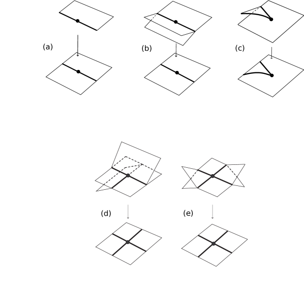
Figure 1. The local forms of Stein factorizations of stable maps from orientable $3$-manifolds to surfaces. The map (symbolized by an arrow) maps from the CW complex $W_{F}$ to $\mathbb{R}^{2}$.

Let $L\subset\mathbb{R}^{3}\subset S^{3}$ be a given link, and let $\overline{L}$ denote a generic projection of it to the plane. Let ${\rm{n}}(L)$ and ${\rm{cr}}(\overline{L})$ denote the number of components of $L$ and the number of crossings of $\overline{L}$, respectively.

Choose a direction in $\mathbb{R}^{2}$, which we represent by a vector $v\in\mathbb{R}^{2}$. We can assume that $v$ satisfies the condition that the projection of the diagram $\overline{L}$ to $\mathbb{R}v^{\bot}$ along $v$ yields only non-degenerate critical points. Let ${\rm{t}}(\overline{L})={\rm{t}}_{v}(\overline{L})$ denote the number of times $\overline{L}$ is tangent to $v$. Suppose at each $v$-tangency $p$ the half line emanating from $p$ in the direction of $v$ avoids the crossings of $\overline{L}$ and intersects $\overline{L}$ transversally (at the points different from $p$). Denote the number of transversal intersections by $\ell(\overline{L},v,p)$. Let $\ell(\overline{L},v)$ denote the maximum of the values $\ell(\overline{L},v,p)$, where $p$ runs over the $v$-tangencies. With these definitions in place now we can state the main result of the paper.

Theorem 1.2.

Suppose that the 3-manifold $M$ is obtained by integral surgery on the link $L\subset S^{3}$. Then there is a stable map $F\colon\thinspace M\to\mathbb{R}^{2}$ such that

1. the Stein factorization $W_{F}$ is homotopy equivalent to the bouquet $\bigvee_{i=1}^{{\rm{n}}(L)}S^{2}$,

2. the number of cusps of $F$ is equal to ${\rm t}_{v}(\overline{L})$,

3. all the non-simple singularities of $F$ are of type (d), and their number is equal to ${\rm cr}(\overline{L})+\frac{3}{2}{\rm t}_{v}(\overline{L})-{\rm n}(L)$,

4. the number of non-simple singularities which are not connected by any singular arc of type (b) to any cusp is equal to ${\rm cr}(\overline{L})+\frac{1}{2}{\rm t}_{v}(\overline{L})-{\rm n}(L)$,

5. the number of simple singularity crossings of $F$ in $\mathbb{R}^{2}$ is no more than

   $$8{\rm cr}(\overline{L})+6\ell(\overline{L},v){\rm t}_{v}(\overline{L})+{\rm t}_{v}(\overline{L})^{2},$$

6. the number of connected components of the singular set of $F$ is no more than ${\rm{n}}(L)+\frac{3}{2}{\rm t}_{v}(\overline{L})+1$, and

7. the maximal number of the connected components of any fiber of $F$ is no more than ${\rm t}_{v}(\overline{L})+3$.

8. Suppose we got $M$ by cutting out and gluing back the regular neighborhood $N_{L}$ of $L$ from $S^{3}$. Then the indefinite fold singular set of $F$ contains a link in $S^{3}-N_{L}$, which is isotopic to $L$ in $S^{3}$ and whose $F$-image coincides with $\overline{L}$.

Remark 1.3.

1. Let $Y$ be a closed orientable $3$-manifold, $f$ a given smooth map of $Y$ into $\mathbb{R}^{2}$ and $L\subset Y$ a link disjoint from the singular set of $f$. Suppose furthermore that $f|_{L}$ is an immersion. Let $M$ denote the $3$-manifold obtained by some integral surgery along $L$. Then the method developed in the proof of Theorem 1.2 provides a stable map of $M$ into $\mathbb{R}^{2}$ (relative to $f$).

2. In constructing the map $F$, the proof of Theorem 1.2 provides a sequence of stable maps $f_{0},f_{1},\ldots,f_{6}$ of $S^{3}$ into $\mathbb{R}^{2}$, where each $f_{i}$ is obtained from $f_{i-1}$ by some deformation, $i=1,\ldots,6$. Finally, the map $F$ is obtained from $f_{6}$. Suppose that $X$ is a compact $4$-manifold which admits a handle decomposition with only $0$- and $2$-handles, i.e. $X$ can be given by attaching 4-dimensional 2-handles to $D^{4}$ along $S^{3}$. Using our method we can construct a stable map $G$ of $X$ into $\mathbb{R}^{2}\times[0,1]$.

Recall that according to [BR74] a closed orientable $3$-manifold $M$ has a stable map into $\mathbb{R}^{2}$ without singularities of types (b), (c), (d) and (e) if and only if $M$ is a connected sum of finitely many copies of $S^{1}\times S^{2}$. According to [Sa96] a closed orientable $3$-manifold $M$ has a stable map into $\mathbb{R}^{2}$ without singular points of types (c), (d) and (e) if and only if $M$ is a graph manifold. By [Le65] a $3$-manifold always has a stable map into $\mathbb{R}^{2}$ without singular points of type (c). Our arguments imply a constructive proof for

Theorem 1.4.

Every closed orientable $3$-manifold has a stable map into $\mathbb{R}^{2}$ without singular points of types (c) and (e).

Remark 1.5.

1. One cannot expect to eliminate the singular points of types (a), (b) or (d) of stable maps from arbitrary closed orientable $3$-manifolds to $\mathbb{R}^{2}$. In this sense our Theorem 1.4 gives the best possible elimination on $3$-manifolds.

2. By taking an embedding $\mathbb{R}^{2}\subset S^{2}$ we get for every closed orientable $3$-manifold a stable map into $S^{2}$ as well without singular points of types (c) and (e). Then by using the method of [Sa06], for example, for eliminating the singular points of type (a), we get a stable map, which is a direct analogue of the indefinite generic maps appearing in [Ba08, Ba09, GK07].

The construction also implies certain relations between quantities one can naturally associate to stable maps and to surgery diagrams.

Definition 1.6.

Suppose that $M$ is a fixed closed, oriented $3$-manifold and $F\colon\thinspace M\to\mathbb{R}^{2}$ is a stable map with singular set $\Sigma$.

• Let ${\rm s}(F)$ denote the number of simple singularity crossings of $F$.

• Let ${\rm ns}(F)$ denote the number of non-simple singularities of $F$.

• Let ${\rm d}(F)$ denote the number of crossing singularities of $F$. Clearly ${\rm s}(F)+{\rm ns}(F)={\rm d}(F)$.

• Let ${\rm nsnc}(F)$ denote the number of non-simple singularities of $F$ which are not connected by any singular arc of type (b) to any cusp.

• Let ${\rm c}(F)$ denote the number of cusps of $F$. Clearly ${\rm nsnc}(F)+{\rm c}(F)\geq{\rm ns}(F)$.

• Let ${\rm cc}(F)$ denote the number of connected components of $F(\Sigma)$. Clearly it is no more than the number of connected components of $\Sigma$.

• Let ${\rm cf}(F)$ denote the maximum number of connected components of the fibers of $F$.

The inequality

$$\operatorname{rank}H_{*}(M)\leq 2{\rm d}(F)+{\rm c}(F)+2{\rm cc}(F)$$

has been shown to hold in [Gr09, Section 2.1]. In addition, by [CT08, Theorem 3.38] we have ${\rm d}(F)\geq||M||/10$, where $||M||$ is the Gromov norm of $M$, cf. also [Gr09, Section 3].

Theorem 1.2 provides several estimates for upper bounds on the topological complexity of smooth maps of a $3$-manifold given by surgery. For example, by summing quantities in Definiton 1.6 and their estimates in Theorem 1.2, we immediately obtain

Corollary 1.7.

Suppose that the 3-manifold $M$ is obtained by integral surgery on the link $L\subset S^{3}$. Let $\overline{L}$ be any diagram of $L$ and $v$ a general position vector in $\mathbb{R}^{2}$. Then

• $\min{\rm d}(F)\leq 9{\rm cr}(\overline{L})+(6\ell(\overline{L},v)+\frac{3}{2}){\rm t}_{v}(\overline{L})+{\rm t}_{v}(\overline{L})^{2}-{\rm n}(L)$,

• $\min{\rm cf}(F)\leq{\rm t}_{v}(\overline{L})+3$,

• $\min\{2{\rm d}(F)+{\rm c}(F)+2{\rm cc}(F)\}\leq 18{\rm cr}(\overline{L})+(12\ell(\overline{L},v)+7){\rm t}_{v}(\overline{L})+2{\rm t}_{v}(\overline{L})^{2}+2$,

where the minima are taken for all the stable maps $F$ of $M$ into $\mathbb{R}^{2}$. Evidently, we can estimate other properties in Definiton 1.6 of stable maps on $M$ as well.

These expressions can be simplified by estimating $\ell(\overline{L},v)$ as

(1.1) $$\ell(\overline{L},v)\leq{\rm t}_{v}(\overline{L})-1$$

cf. Lemma 3.7.

The number of tangencies of a projection of a knot in a fixed direction is reminiscent to the number of cusp singularities of a front projection of a Legendrian knot in the standard contact 3-space. Based on this analogy, our previous results imply an estimate on a quantity attached to a Legendrian knot in the following way.

Recall first that the standard contact structure $\xi_{st}$ on $\mathbb{R}^{3}$ is the 2-plane field given by the kernel of the 1-form $\alpha=dz+xdy$. A knot ${\mathcal{L}}$ is Legendrian if the tangent vectors of ${\mathcal{L}}$ are in $\xi_{st}$. (To indicate the Legendrian structure on the knot, we will denote it by ${\mathcal{L}}$ and reserve the notation $L$ for smooth knots and links.) If ${\mathcal{L}}$ is chosen generically within its Legendrian isotopy class, its projection to the $(y,z)$ plane will have no vertical tangencies, and at any crossing the strand with smaller slope will be over the one with higher slope. Consider now a Legendrian knot ${\mathcal{L}}$ and let ${\overline{\mathcal{L}}}$ denote such a projection (called a front projection) of ${\mathcal{L}}$. The Thurston-Bennequin number ${\rm{tb}}({\mathcal{L}})$ of ${\mathcal{L}}$ is given by the formula $w({\overline{\mathcal{L}}})-\frac{1}{2}(\#cusps({\overline{\mathcal{L}}}))$, where $w({\overline{\mathcal{L}}})$ stands for the writhe (i.e. the signed sum of the double points) of the projection. Although the definition of tb$({\mathcal{L}})$ uses a projection of the Legendrian knot ${\mathcal{L}}$, it is not hard to show that the resulting number is an invariant of the Legendrian isotopy class of ${\mathcal{L}}$.

In case the projection has only negative crossings, we have that $w({\overline{\mathcal{L}}})=-{\rm{cr}}({\overline{L}})$, hence the resulting Thurston-Bennequin number can be identified with $-{\rm cr}(\overline{L})-\frac{1}{2}{\rm{t}}_{v}(\overline{L})$ after choosing $v$ appropriately, cf. [Ge08, OS04]. (In this case the generic projection ${\overline{L}}$ used in the definitions of ${\rm{t}}_{v}(\overline{L})$ and ${\rm{cr}}({\overline{L}})$ is derived from the front projection ${\overline{\mathcal{L}}}$ by rounding the cusps.)

As it is customary, we define ${\rm{TB}}(L)$ as the maximum of all Thurston-Bennequin numbers of Legendrian knots smoothly isotopic to $L$. (It is a nontrivial fact, and follows from the tightness of $\xi_{st}$ that this maximum exists.) A modification of this definition for negative knots (i.e. for knots admitting projections with only negative crossings) provides

Definition 1.8.

For a negative knot $L\subset\mathbb{R}^{3}$ let ${\rm TB}^{-}(L)$ denote the value $\max\{{\rm tb}({\mathcal{L}})\}$ where ${\mathcal{L}}$ runs over those Legendrian knots smoothly isotopic to $L$ which admit front diagrams with only negative crossings.

It is rather easy to see that if the knot $L$ admits a projection with only negative crossings, then it also has a front projection with the same property. Clearly ${\rm TB}^{-}(L)\leq{\rm TB}(L)$.

Theorem 1.9.

For a negative knot $L\subset\mathbb{R}^{3}$ and any $3$-manifold $M$ obtained by an integral surgery along $L$ we have

• ${\rm TB}^{-}(L)\leq-\min\frac{\sqrt{{\rm s}(F)}}{2\sqrt{7}}$,

• ${\rm TB}^{-}(L)\leq-\min\frac{\sqrt{{\rm d}(F)}}{2\sqrt{7}}$,

• ${\rm TB}^{-}(L)\leq-\min{\rm nsnc}(F)-1$,

where the minima are taken for all the stable maps $F$ of $M$ into $\mathbb{R}^{2}$.

By Theorem 1.9 and [CT08, Theorem 3.38] we obtain

Corollary 1.10.

For a negative knot $L\subset\mathbb{R}^{3}$ and any $3$-manifold $M$ obtained by an integral surgery along $L$, we have ${\rm TB}^{-}(L)\leq-\frac{\sqrt{||M||}}{2\sqrt{70}}$.

Acknowledgements: The authors were supported by OTKA NK81203 and by the Lendület program of the Hungarian Academy of Sciences. The first author was partially supported by Magyary Zoltán Postdoctoral Fellowship. The authors thank the anonymous referee for the comments which improved the paper.

2. Preliminaries

In this section, we recall and summarize some technical tools. First, we show that a cusp can be pushed through an indefinite fold arc as in Figure 2:

Lemma 2.1 (Moving cusps).

Suppose that in a neighborhood $U$ of a point $p\in M$ the Stein factorization of a map $f\colon\thinspace M\to\mathbb{R}^{2}$ is given by Figure 2(a). Then $f$ can be deformed in this neighborhood to a map $f^{\prime}$ so that the Stein factorization of $f^{\prime}$ is as the diagram of Figure 2(b).

Proof.

Suppose $q\in M$ is the cusp singular point and $\alpha\subset M$ is the indefinite fold arc at hand. Let $x\in\mathbb{R}^{2}$ be a point on the other side of $f(\alpha)$ in $f(U)$. Connect $f(q)$ and $x$ by an embedded arc $\beta^{\prime}$. Then there is an arc $\beta\subset M$ such that $f(\beta)=\beta^{\prime}$, $\beta$ starts at $q$ and $\beta$ and $\alpha$ do not intersect. By using the technique of [Le65] we can now deform $f$ in a small tubular neighborhood of $\beta$ to achieve the claimed map $f^{\prime}$. Note that during this move one singular point of type (d) appears. ∎

An analogous statement holds if we move a cusp from a $1$-sheeted region to a $2$-sheeted region.

Figure 2. Moving cusps. A map can be deformed so that the image of a cusp point goes to the other side of the image of an indefinite fold arc.

According to the next result, two cusps can be eliminated as in Figure 3:

Lemma 2.2 (Eliminating cusps).

Suppose that in a neighborhood $U$ of a point $p\in M$ the Stein factorization of a map $f\colon\thinspace M\to\mathbb{R}^{2}$ is given by Figure 3(a). Then $f$ can be deformed in this neighborhood to a map $f^{\prime}$ so that the Stein factorization of $f^{\prime}$ is as the diagram of Figure 3(b).

Proof.

This statement is the elimination in [Le65, pages 285–295] for $3$-dimensional source manifolds. ∎

Figure 3. Eliminating cusps.

Recall that if $f\colon\thinspace M\to\mathbb{R}^{2}$ is a stable map and $S_{f}\subset M$ denotes its singular set, then $f|_{S_{f}}$ is a generic immersion with cusps, i.e. if $C_{f}\subset M$ denotes the set of cusp points, then $f|_{S_{f}-C_{f}}$ is a generic immersion with finitely many double points and $f|_{C_{f}}$ is disjoint from $f|_{S_{f}-C_{f}}$.

The following result will be the key ingredient in our subsequent arguments for proving Theorem 1.2.

Lemma 2.3 (Making wrinkles).

Suppose that $f\colon\thinspace M\to\mathbb{R}^{2}$ is a stable map and let $L\subset M$ denote an embedded closed $1$-dimensional manifold such that $L$ is disjoint from the singular set $S_{f}$, $f|_{L}$ is a generic immersion and $f|_{L\cup S_{f}}$ is a generic immersion with cusps. Let $N_{L}$ be a small tubular neighborhood of $L$ disjoint from $S_{f}$ and fix an identification of $N_{L}$ with the normal bundle of $L$. Let $s\colon\thinspace L\to N_{L}$ be a non-zero section such that $f(s(x))\neq f(x)$ for any $x\in L$. Then $f$ is homotopic to a smooth stable map $f^{\prime}$ such that

1. $f=f^{\prime}$ outside $N_{L}$,

2. the singular set of $f^{\prime}$ is $S_{f}\cup L\cup s(L)$,

3. $f^{\prime}$ has indefinite fold singularities along $L$,

4. $f^{\prime}$ has definite fold singularities along $s(L)$,

5. $f^{\prime}|_{L}=f|_{L}$,

6. $f^{\prime}|_{s(L)}$ is an immersion parallel to $f|_{L}$ and

7. if for a double point $y$ of $f|_{L}$ the two points in $f^{-1}(y)\cap L$ lie in the same connected component of the fiber $f^{-1}(y)$, then the double point $y$ of $f^{\prime}|_{L}$ correspond to a singularity of type (d).

Proof.

We perform the homotopy inside $N_{L}$ fiberwise as shown by Figure 4. Since $N_{L}$ is the trivial bundle, the homotopy of the fibers yields a homotopy of the entire $N_{L}$. ∎

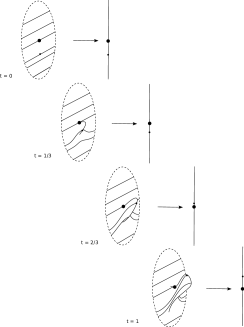
Figure 4. The deformation of $f$ to $f^{\prime}$ in a fiber of $N_{L}$.

Remark 2.4.

If the submanifold $L$ has boundary, we can still get something similar. In this case the section $s$ should be zero at the boundary points of $L$, and the homotopy yields a stable map $f^{\prime}$ with cusps at $\partial L$.

3. Proof of the results

3.1. Construction of the stable map on $M$

Proof of Theorem 1.2.

We will prove the theorem by presenting an algorithm which produces the map $F$ on $M$ with the desired properties. This algorithm will be given in seven steps; the first six of these steps are concerned with maps on $S^{3}$. Let us start with a fold map $f_{0}\colon\thinspace S^{3}\to\mathbb{R}^{2}$ with one unknotted circle $C\subset S^{3}$ as singular set such that $f_{0}|_{C}$ is an embedding and $f_{0}^{-1}(p)$ is a circle for each regular point $p\in f_{0}(S^{3})$. Then the Stein factorization of $f_{0}$ is a disk together with its embedding into $\mathbb{R}^{2}$. By cutting out the interior of a sufficiently small tubular neighborhood $N_{C}$ of $C$ from $S^{3}$, we get a solid torus $S^{3}-{\rm{int}}\,N_{C}$ whose boundary is mapped into $\mathbb{R}^{2}$ by $f_{0}$ as a circle fibration over a circle parallel to $f_{0}(C)$, and $f_{0}|_{S^{3}-{\rm{int}}\,N_{C}}$ is a trivial circle bundle $S^{1}\times D^{2}\to D^{2}$. Suppose the link $L\subset S^{3}$ is disjoint from $N_{C}\cup\{1\}\times D^{2}$. Then by identifying $S^{3}-(N_{C}\cup\{1\}\times D^{2})$ with $\mathbb{R}^{3}$ and $f_{0}|_{S^{3}-(N_{C}\cup\{1\}\times D^{2})}$ with the projection onto $\mathbb{R}^{2}$, we get a link diagram $\overline{L}=f_{0}(L)$. Now we start modifying this map $f_{0}$. In Steps 1 through 6 we will deal with maps on $S^{3}$, and the goal will be to obtain a map which is suitable with respect to the fixed surgery link $L$. In particular, we aim to find a map on $S^{3}$ with the property that its restriction to any component of $L$ is an embedding into $\mathbb{R}^{2}$. We suppose that the modifications through Step 1, …, Step 6 happen so that all the images of the maps $f_{1}$, …, $f_{6}$ lie completely inside the disk determined by the (unchanged) circle $f_{i}(C)$, $i=1,\ldots,6$. This can be reached easily by choosing $f_{0}(C)$ to bound an area “large enough” in $\mathbb{R}^{2}$ and supposing that the diameter of $\overline{L}$ is small.

Step 1

Our first goal is to deform $f_{0}$ so that the resulting map $f_{1}$ has fold singularities along $L$. Apply Lemma 2.3 to the map $f_{0}\colon\thinspace S^{3}\to\mathbb{R}^{2}$ and the embedded $1$-dimensional manifold $L\subset S^{3}$, and denote the resulting stable map by $f_{1}$. It is a fold map, its indefinite fold singular set is $L$ and its definite fold singular set is $C\cup L^{\prime}$, where $L^{\prime}=s(L)$ is isotopic to $L$; for an example see Figure 5.

Figure 5. The image of the singular set of the map $f_{1}\colon\thinspace S^{3}\to\mathbb{R}^{2}$, where $L$ is the trefoil knot. The outer circle is $f_{1}(C)$, the inner solid curve is $f_{1}(L^{\prime})$ and the dashed curve is $f_{1}(L)$. The double points of $f_{1}(L)$ correspond to singularities of type (d).

Since $L^{\prime}$ is isotopic to $L$, the integral surgery along $L$ giving $M$ can be equally performed along $L^{\prime}$. Recall that doing surgery along $L^{\prime}$ simply means that we cut out a tubular neighborhood of the definite fold curve $L^{\prime}$ (which is diffeomorphic to $L^{\prime}\times D^{2}$), and glue it back by a diffeomorphism of its boundary $L^{\prime}\times S^{1}$. If the image $f_{1}(L^{\prime})$ was an embedding of circles, then it would be easy to construct the claimed map $F$ on the $3$-manifold given by the integral surgery. Since this is not the case in general, we need to further deform the map $f_{1}$.

Let $B$ denote the interior of the bands (one for each component of $L$) bounded by $q_{f_{1}}(L)$ and $q_{f_{1}}(L^{\prime})$ in the Stein factorization $W_{f_{1}}$. Then $B$ is immersed into $\mathbb{R}^{2}$ by $\bar{f}_{1}$. The Stein factorizations of the maps $f_{2},\ldots,f_{6}$ in the next steps will be built on $B$. Let $B^{\prime}$ denote the surface $W_{f_{1}}-{\rm cl}B$.

Step 2

Now, our goal is to deform $f_{1}$ so that the Stein factorization of the resulting map $f_{2}$ has small “flappers” near $q_{f_{2}}(L^{\prime})$ at the points where $\bar{f}_{2}(q_{f_{2}}(L^{\prime}))$ is tangent to the general position vector $v$. These “flappers” will help us to move the image of $L$ so that it will become an embedding into $\mathbb{R}^{2}$.

First, we use Lemma 2.3 together with Remark 2.4 as follows. Let $T$ be the set of points in $q_{f_{1}}(L^{\prime})$ such that for each $p\in T$ the direction $v$ is tangent to $f_{1}(L^{\prime})$ at $\bar{f}_{1}(p)$. For each $p\in T$ take a small embedded arc $\alpha_{p}$ in a small neighborhood of $p$ in $B$ such that $\bar{f}_{1}|_{\alpha_{p}}$ is an embedding parallel to $f_{1}(L)$. For each arc $\alpha_{p}$ there exists an embedded arc $\tilde{\alpha}_{p}$ in $S^{3}$ such that $q_{f_{1}}|_{\tilde{\alpha}_{p}}$ is an embedding onto $\alpha_{p}$. See, for example, the upper picture of Figure 6, where the small dashed arcs having cusp endpoints represent the arcs $f_{1}(\tilde{\alpha}_{p})=\bar{f}_{1}(\alpha_{p})$ for all $p\in T$.

Figure 6. We obtain the upper picture by applying Lemma 2.3 and Remark 2.4 to the small arcs $\{\tilde{\alpha}_{p}:p\in T\}$ in $S^{3}$ which are mapped by $f_{1}$ to the dashed arcs near the points of the diagram $\overline{L}$ where it is tangent to $v$. We obtain the lower picture by applying Lemma 2.3 and Remark 2.4 to the new arcs added to the upper picture. The solid arcs correspond to singularities of type (a) and the black double points of the dashed arcs correspond to singularities of type (d).

Apply Lemma 2.3 and Remark 2.4 to the map $f_{1}\colon S^{3}\to\mathbb{R}^{2}$ and the arcs $\{\tilde{\alpha}_{p}\subset S^{3}:p\in T\}$ to obtain a map $f_{1}^{\prime}$. The section $s$ in Lemma 2.3 is chosen so that if we project the $f_{1}^{\prime}$-images of the arising new definite fold curves in $\mathbb{R}^{2}$ to $\mathbb{R}v$, then for each curve there is only one critical point, which is a maximum. An example for the resulting map $f_{1}^{\prime}$ can be seen in the upper picture of Figure 6. Note that the deformation yielded small “flappers” in $W_{f_{1}^{\prime}}$ attached to $B$ along the arcs $\{\alpha_{p}:p\in T\}$. Next, for each $p\in T$ take small arcs $\beta_{p}$ in $W_{f_{1}^{\prime}}$ which intersect generically the previous arcs $\{\alpha_{p}:p\in T\}$, lie in $B$ and on the “flappers” and are mapped into $\mathbb{R}^{2}$ almost parallel to $v$. See the new small dashed arcs in the lower picture of Figure 6. Once again, there are small arcs $\{\tilde{\beta}_{p}:p\in T\}$ embedded in $S^{3}$ mapped by $f_{1}^{\prime}$ onto $\{\beta_{p}:p\in T\}$, respectively.

The application of Lemma 2.3 and Remark 2.4 for these arcs provides us a map, which we denote by $f_{2}$. This map will have one additional flapper for every flapper of $f_{1}^{\prime}$. We choose the section $s$ in Lemma 2.3 so that the $f_{2}$-images of the arising new definite fold curves lie inward from the arcs $\{\bar{f}_{1}^{\prime}(\beta_{p}):p\in T\}$, respectively, in the $\bar{f}_{2}$-image of $B$ and the previous flappers. For an enlightening example, see the lower picture of Figure 6. Note that after this step $|T|$ new singular points of type (d) appeared. Also note that for each $p\in T$ we have four cusp singular points in $S^{3}$, three of which are mapped by $q_{f_{2}}$ into $B$. We denote the set of these three cusps by $C_{p}$. For each $p\in T$ the $f_{2}$-images of two of these three cusps in $C_{p}$ point to the direction $-v$. We denote the set of these two cusps by $D_{p}$. Note that the definite fold curves in the images of the two cusps in $D_{p}$ are on opposite sides.

Step 3

Now our goal is to obtain definite fold arcs connecting points of $S^{3}$ where $f_{2}$ had cusps. Moreover these definite fold arcs will be mapped into $\mathbb{R}^{2}$ parallel to the diagram $\overline{L}$. (These curves will be translated in the next step so that later they will lead to an embedding of $L$ into $\mathbb{R}^{2}$.)

In order to reach this goal, we deform the map $f_{2}\colon\thinspace S^{3}\to\mathbb{R}^{2}$ further by eliminating half of the cusps as follows. We proceed for each component of $L$ separately and in the same way, thus in the following we can suppose that $L$ is connected. Take a cusp $q_{0}\in S^{3}$ which is in $C_{x}-D_{x}$ for an $x\in T$ such that the entire $f_{2}(L^{\prime})$ lies to the right hand side of its tangent at $\bar{f}_{2}(x)$. By going along the band $B$ in $W_{f_{2}}$ in the direction to which the $f_{2}$-image of this cusp $q_{0}$ points, we reach another cusp $q_{1}$ in $C_{p}$ for some $p\in T$ at the next $v$-tangency of $f_{2}(L^{\prime})$. If this cusp does not belong to $D_{p}$, then it is possible to apply Lemma 2.2 and eliminate these two cusps, since they are in the position of Figure 3. Then we continue by taking the cusp in $D_{p}$ whose Stein factorization is folded inward. If the cusp $q_{1}$ does belong to $D_{p}$, then we choose that cusp from $D_{p}$ which can be used to eliminate $q_{0}$ (it is easy to see that this is exactly the cusp in $D_{p}$ whose Stein factorization is folded inward), we eliminate them, then we continue by taking the cusp belonging to $C_{p}-D_{p}$. This procedure goes all along the band $B$, meets all $p\in T$ and eliminates half of the cusps. After finishing this process, we obtain a stable map, which we denote by $f_{3}$; cf. Figure 7 for an example.

Figure 7. Eliminating half of the cusps in the lower picture of Figure 6. The black double points correspond to singularities of type (d).

The cusp elimination results new definite fold curves whose $f_{3}$-image is an immersion, and which have double points near the crossings of the diagram $\overline{L}$. In the next step we will deform $f_{3}$ so that the double points of these new curves will be localized near the images of the remaining cusps.

Step 4

Now our goal is to deform $f_{3}$ to a map $f_{4}$ such that the definite fold arcs obtained in the previous step will be mapped into $\mathbb{R}^{2}$ far from the diagram $\overline{L}$. (Informally, we will “lift” some of the arcs in the direction of $v$.) Moreover, the immersion of these definite fold arcs into $\mathbb{R}^{2}$ will have double points only near some cusps of $f_{4}$. This brings us closer to the original goal to have a map which embeds a link isotopic to $L$ into the plane.

The cusp eliminations above affect only small tubular neighborhoods of curves connecting cusps in $S^{3}$. Denote by $\delta\subset S^{3}$ the new definite fold arcs which appear in these tubular neighborhoods after the eliminations. Note that by the algorithm above, the arcs $\delta$ are mapped into $\mathbb{R}^{2}$ so that by an elementary deformation they can be moved “upward” in the direction of $v$, see Figure 7.

So we further deform $f_{3}\colon\thinspace S^{3}\to\mathbb{R}^{2}$ to get a stable map denoted by $f_{4}$ as indicated in Figure 8: as it is shown by the picture, the arcs are “lifted”. In fact, we deform $\bar{f}_{3}$: we move the top of the “flappers” corresponding to the $\alpha$-curves of Step 2 and the $\bar{f}_{3}$-image of the curves $q_{f_{3}}(\delta)$ in the direction of $v$ and far from $f_{3}(L)$. We proceed for each component of $L$ separately and in the same way, thus in the following we can suppose that $L$ is connected. First we choose a point $x\in T$ such that the entire $f_{3}(L^{\prime})$ lies to the right hand side from its tangent at $\bar{f}_{3}(x)$. Then, by walking along the band $B\subset W_{f_{3}}$ starting from $x$, we deform the flappers and the curves $\bar{f}_{3}(q_{f_{3}}(\delta))$ to be mapped into the plane as a “zigzag” far away from the diagram $\overline{L}$. More precisely, consider the coordinate system in $\mathbb{R}^{2}$ with origin $x$ and coordinate axes $\mathbb{R}v^{\perp}$ and $\mathbb{R}v$, respectively, where $v^{\perp}$ denotes the vector obtained by rotating $v$ clockwise by $90$ degrees. By extending the $\bar{f}_{3}$-image of the flappers in the direction of $v$ deform the $\bar{f}_{3}$-image of the curves $q_{f_{3}}(\delta)$ so that by going along $B$ between the points $p_{i},p_{i+1}\in T$, where $1\leq i\leq|T|-1$ and $p_{1}=x$, the corresponding component of the curve $f_{3}(\delta)$ is mapped into a small tubular neighborhood of a line with slope $(-1)^{i+1}$ for $i=1,\ldots,|T|-1$. Finally, arrange the last component of ${f_{3}}(\delta)$ starting with slope $-1$ and ending at the first (extended) flapper belonging to $x$, see Figure 8.

Note that as a result the double points of the immersion of the deformed curves $f_{4}(\delta)$ are in a small neighborhood of the cusps mapped close to the tops of the flappers.

Figure 8. The Stein factorization of $f_{4}$, i.e. the deformation of $f_{3}$ of Figure 7. (The straight line represents the line $l$ used to cut $W_{f_{4}}$ in Step 5.) The upper part of $W_{f_{4}}$ from the bold $1$-complex is denoted by $A$. (As usual, the circle $f_{4}(C)$ is omitted.)

Step 5

In this step, we modify the stable map $f_{4}$ so that the cusps of the resulting map $f_{5}$ will be easy to eliminate in the next step. Let $l\subset\mathbb{R}^{2}$ be a line perpendicular to $v$ located near $\bar{f}_{4}(B)$, separating it from the other parts moved to the direction of $v$ in Step 4, as indicated in Figure 8.

Now, we cut the $2$-complex $W_{f_{4}}-B^{\prime}$ (recall that $B^{\prime}$ denotes $W_{f_{1}}-{\rm cl}B$, see Step 1) along the $\bar{f}_{4}$-preimage of the line $l$, thus we obtain the decomposition

$$W_{f_{4}}=A\cup_{\bar{f}_{4}^{-1}(l)\cap(W_{f_{4}}-B^{\prime})}A^{\prime},$$

where $A^{\prime}$ denotes the $2$-dimensional CW complex containing $q_{f_{4}}(L)$ and $A$ denotes the closure of $W_{f_{4}}-A^{\prime}$. Then $q_{f_{4}}^{-1}(A)$ is a $3$-manifold with boundary. Let us denote the $1$-complex $q_{f_{4}}(\partial q_{f_{4}}^{-1}(A))$ by $\partial A$. In order to visualize $\partial A$ in Figure 8, we suppose that the cutting of $W_{f_{4}}$ along $\bar{f}_{4}^{-1}(l)\cap(W_{f_{4}}-B^{\prime})$ is a little bit perturbed and thus the bold $1$-complex in Figure 8 represents $\partial A$. Before proceeding further, we need a better understanding of the $q_{f_{4}}$-preimages of the sets appearing in the above decomposition. The preimage $q_{f_{4}}^{-1}(\partial A)$ is clearly diffeomorphic to $J\times S^{1}$ for a link $J\subset S^{3}$. The following statements show much more about $q_{f_{4}}^{-1}(\partial A)$. It is easy to see that the numbers of components of $J$ and $L$ are equal. However, we have the stronger

Lemma 3.1.

A longitudinal curve in $q_{f_{4}}^{-1}(\partial A)$ is isotopic to $L$.

Proof.

The $1$-complex $\partial A$ decomposes as a union of $1$-cells: some of them (which we depict as “small $1$-cells” in Figure 8) are attached at one of their endpoints to the union of the other 1-cells, we denote these small cells by $\sigma_{i}$ for $i=1,\ldots,{|T|}$. Others are attached by both of their endpoints. Let $\sigma$ denote the $1$-complex $\partial A-\bigcup_{i=1}^{|T|}\sigma_{i}$. Then the PL embedding $\sigma\subset W_{f_{4}}$ is isotopic to the subcomplex $\iota$ of $W_{f_{4}}$ formed by the arcs of type (b) in the open bands $B$ connecting the singular points of type (d) in $B$. Furthermore, the subcomplex $\iota$ is isotopic to $q_{f_{4}}(L^{\prime})$. Take a small closed regular neighborhood $N$ of $q_{f_{4}}(L^{\prime})$. Then $q_{f_{4}}^{-1}(N)$ is naturally a $D^{2}$-bundle over $L^{\prime}$. The boundary of $N$ in $W_{f_{4}}$ is a $1$-manifold isotopic to $q_{f_{4}}(L^{\prime})$, and we will denote it by $\lambda$. Clearly $q_{f_{4}}^{-1}(\lambda)$ is diffeomorphic to $L^{\prime}\times S^{1}$. Note that any section of $q_{f_{4}}^{-1}(\lambda)$ is isotopic to $L^{\prime}$.

The isotopy between $\lambda$ and $\iota$ and the isotopy between $\iota$ and $\sigma$ can be chosen easily so that they give a PL embedding $\varepsilon\colon\thinspace S^{1}\times[0,1]\to W_{f_{4}}$ such that $S^{1}\times\{0\}$ and $S^{1}\times\{1\}$ correspond to $\lambda$ and $\sigma$, respectively. For $j=1,\ldots,|T|$, let $U_{j}$ denote small regular neighborhoods of the singular points of type (d) located near the cusp points in $B$ in $W_{f_{4}}$, such a $U_{j}$ and the restriction $\bar{f}_{4}|_{U_{j}}$ can be seen in Figure 1(d). Then the intersection $\varepsilon(S^{1}\times[0,1])\cap(\bigcup_{j=1}^{|T|}U_{j})$ consists of a union of disks, which will be denoted by $\bigcup_{j=1}^{|T|}D_{j}$.

First, observe that for each $j=1,\ldots,|T|$ there exists a disk $\tilde{D}_{j}$ embedded into $q_{f_{4}}^{-1}(U_{j})$ in $S^{3}$ whose boundary $\partial\tilde{D}_{j}$ is mapped by $q_{f_{4}}$ homeomorphically onto the boundary $\partial D_{j}$, i.e. $\partial\tilde{D}_{j}$ is a lifting of $\partial D_{j}$. To see this, consider the $3$-manifold $q_{f_{4}}^{-1}(U_{j})$ for each $j=1,\ldots,|T|$. By [Le85] the manifold $q_{f_{4}}^{-1}(U_{j})$ is diffeomorphic to $R\times[0,1]$, where $R$ is a disk with three holes and it is mapped by ${f_{4}}$ into $\mathbb{R}^{2}$ as we can see in Figure 9(a).

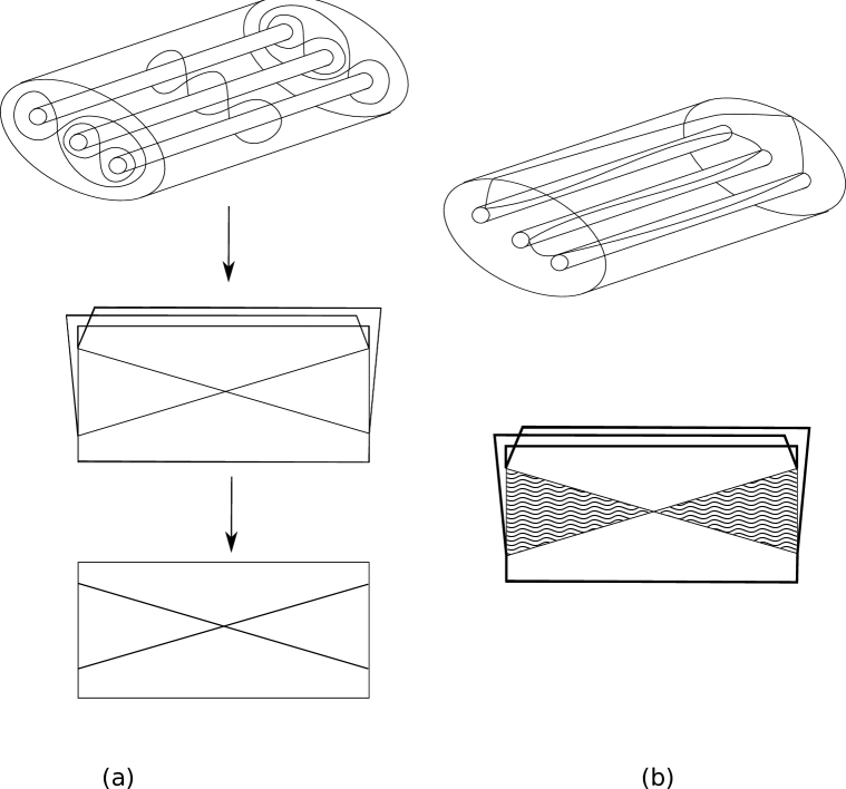
Figure 9. In (a) we can see the manifold $R\times[0,1]$ and how it is mapped onto the regular neighborhood $U_{j}$ and into $\mathbb{R}^{2}$, cf. Figure 1(d). $R\times\{0\}$ is mapped onto the left side of the rectangle $\bar{f}_{4}(U_{j})$ as a proper Morse function with two indefinite critical points. The two “figure eights” in $R\times\{0\}$ are the two singular fibers. $R\times\{1\}$ is mapped similarly onto the right side of $\bar{f}_{4}(U_{j})$. The middle fiber in $R\times[0,1]$ is mapped to the singular point of type (d). For a detailed analysis see [Le85]. In (b) we can see the boundary $\partial\tilde{D}_{j}$ in $R\times[0,1]$ and its image in $U_{j}$ represented by a bold $1$-complex.

Each disk $D_{j}$ can be located in $U_{j}$ essentially in four ways, for example the lower picture of Figure 9(b) shows the disk $D_{j}$ for the leftmost non-simple singularity crossing of type (d) in Figure 8. We get $D_{j}$ on the picture by cutting out the two shaded areas from the $2$-complex $U_{j}$. It is easy to see in the upper picture of Figure 9(b) how to put the disk $\tilde{D}_{j}$ into $R\times[0,1]$. The other three possibilities for the location of a disk $D_{j}$ in $U_{j}$ and the disk $\tilde{D}_{j}$ in $q_{f_{4}}^{-1}(U_{j})$ can be described in a similar way.

Now observe that $\varepsilon(S^{1}\times[0,1])-\bigcup_{j=1}^{|T|}D_{j}$ can be lifted to $S^{3}$ extending $\bigcup_{j=1}^{|T|}\tilde{D}_{j}$ because of the following. First, the regular neighborhoods of the singular points of type (c) in $B$ (see Figure 1(c)) intersect $\varepsilon(S^{1}\times[0,1])$ in disks which can be lifted to $S^{3}$. Then the intersection of the small regular neighborhoods of the singular curves of type (b) and $\varepsilon(S^{1}\times[0,1])$ can be lifted as well since there is no constraint for the lift at the regular points of $f_{4}$. Finally observe that the rest of $\varepsilon(S^{1}\times[0,1])$ intersects $W_{f_{4}}$ only in areas of non-singular points which are attached to the boundary of $\varepsilon(S^{1}\times[0,1])$, so the previous lifts extend over the entire $\varepsilon(S^{1}\times[0,1])$.

Hence we obtain an embedding $\tilde{\varepsilon}\colon\thinspace S^{1}\times[0,1]\to S^{3}$ with $S^{1}\times\{0\}$ and $S^{1}\times\{1\}$ corresponding to lifts of $\lambda$ and $\sigma$, respectively. Thus we obtain an isotopy between a longitude of $q_{f_{4}}^{-1}(\partial A)$ and a lift of $\lambda$. The fact that any lift of $\lambda$ is isotopic to $L^{\prime}$ finishes the proof. ∎

Figure 10.

Lemma 3.2.

The preimage $q_{f_{4}}^{-1}(A)$ is isotopic to a regular neighborhood of $L$.

Proof.

It is enough to show that $q_{f_{4}}^{-1}(A)$ is diffeomorphic to $L\times D^{2}$ extending naturally the $L\times S^{1}$ structure on its boundary since by Lemma 3.1 the union of tori $\partial q_{f_{4}}^{-1}(A)$ contains a longitude isotopic to $L$. Moreover it is enough to show that the $q_{f_{4}}$-preimage of the part of $A$ homeomorphic to the CW complex in Figure 10 is diffeomorphic to $[0,1]\times D^{2}$, where the $q_{f_{4}}$-preimage of the two vertical edges on the right-hand side of the $2$-complex of Figure 10 corresponds to $\{0,1\}\times D^{2}$. Clearly the $q_{f_{4}}$-preimage of the two vertical edges on the right-hand side is diffeomorphic to $\{0,1\}\times D^{2}$ since $q_{f_{4}}^{-1}(x)$ is a circle for any $x$ lying in the two vertical edges except if $x$ is one of the two top ends. If $x$ is one of the two top ends, then $q_{f_{4}}^{-1}(x)$ is one point since it is a definite fold singularity. The $q_{f_{4}}$-preimage of the backward sheet in Figure 10 is diffeomorphic to $[0,1]\times D^{2}$ minus $I\times D^{2}$ for an interval $I$. The $q_{f_{4}}$-preimage of the forward sheet is diffeomorphic to $I\times D^{2}$. ∎

Corollary 3.3.

Any longitudinal curve in $q_{f_{4}}^{-1}(\partial A)$ is isotopic to $L$.

In order to obtain the map $f_{5}$, we modify the map $f_{4}|_{q_{f_{4}}^{-1}(A)}\colon\thinspace L\times D^{2}\to\mathbb{R}^{2}$ outside a neighborhood of $q_{f_{4}}^{-1}(\partial A)$ as it is shown by Figure 11: our goal is to have the arrangement that if for a cusp singularity $q_{1}\in S^{3}$ the point $q_{f_{5}}(q_{1})$ is connected in $W_{f_{5}}-A^{\prime}$ to $\partial A$ by a $1$-cell $\gamma$ mapped into $\mathbb{R}^{2}$ parallel to $v$ and $\gamma$ corresponding to an indefinite fold curve, then a definite fold curve should connect $q_{1}$ to another cusp $q_{2}$ with the same property for $q_{f_{5}}(q_{2})$. Thus we obtain a map $f_{5}$ such that $q_{f_{5}}^{-1}(W_{f_{5}}-A^{\prime})$ is isotopic to a regular neighborhood of $L$ by the same argument as in Lemma 3.2. Also $q_{f_{5}}^{-1}(W_{f_{5}}-A^{\prime})$ coincides with $q_{f_{4}}^{-1}(A)$ and $f_{5}$ coincides with $f_{4}$ in a neighborhood of $q_{f_{5}}^{-1}(A^{\prime})$.

We arrange the cusps of $f_{5}$ in $q_{f_{4}}^{-1}(A)$ to form pairs as follows. In $W_{f_{5}}$ sheets are attached to $B$ along arcs of type (b) (possibly containing points of type (c) at some endpoints). Walking along the bands $B$ and restricting ourselves to the intersection of the sheets and $W_{f_{5}}-A^{\prime}$, we have that every sheet contains a pair of cusps and every second sheet contains a singular arc of type (a) connecting its pair of cusps, for example, see Figure 11.

Figure 11. The Stein factorization of $f_{5}|_{q_{f_{5}}^{-1}(W_{f_{5}}-A^{\prime})}\colon\thinspace L\times D^{2}\to\mathbb{R}^{2}$. There are two $\mathcal{P}$-pairs of cusps.

A natural pairing is that two cusps form a pair if they are in the same sheet and they are connected by a singular arc of type (a). We refer to this pairing as $\mathcal{Q}$-pairing. We also define another pairing $\mathcal{P}$: two cusps form a $\mathcal{P}$-pair if they are in the same sheet and they are not connected by any singular arc of type (a).

Step 6

In this step, we eliminate the cusps of $f_{5}$ contained in $q_{f_{5}}^{-1}(W_{f_{5}}-A^{\prime})$. These cusps are mapped by $f_{5}$ in the direction of $v$ far from $\overline{L}$ and arranged into $\mathcal{P}$-pairs in the previous step. The restriction of the resulting map $f_{6}\colon\thinspace S^{3}\to\mathbb{R}^{2}$ to a link isotopic to $L$ will be an embedding. (Hence after this step the construction of the claimed map $F$ on $M$ will be easy.)

We have exactly $|T|/2$ $\mathcal{P}$-pairs of cusps in $q_{f_{5}}^{-1}(W_{f_{5}}-A^{\prime})$. Observe that for each component of $L$ one $\mathcal{P}$-pair can be eliminated immediately: for example in Figure 11 the pair on the “highest” sheet is in the sufficient position to eliminate. In the following, we deal with the other $\mathcal{P}$-pairs.

More concretely, we perform the deformations and the eliminations of the pairs of cusps of $f_{5}$ in $q_{f_{4}}^{-1}(A)$ as shown in Figure 12 as follows.

Figure 12. Moving and eliminating the cusps. We move and eliminate the $\mathcal{P}$-pair of cusps along the arrows. The dashed arcs represent $1$-complexes used to deform $\sigma$ in the proof of Lemma 3.4.

First, by using Lemma 2.1 we move each pair of cusps having the position as in Figure 12(a) to the position as in Figure 12(b) thus creating a singularity of type (d). Then by using Lemma 2.2 we eliminate each pair of cusps, see Figures 12(b) and 12(c).

The resulting map will be denoted by $f_{6}$ (see Figure 13). Notice that $f_{6}$ and $f_{5}$ coincide in a neighborhood of $q_{f_{5}}^{-1}(A^{\prime})$. The deformations above yield definite fold curves $K\subset S^{3}$, whose image under $f_{6}$ is an embedding into $\mathbb{R}^{2}$ as indicated in Figure 13 by the bold curve.

Figure 13. The Stein factorization of the stable map $f_{6}\colon\thinspace S^{3}\to\mathbb{R}^{2}$. (The circle $f_{6}(C)$ is omitted.)

Lemma 3.4.

The link $K$ is isotopic to $L$.

Proof.

By Lemma 3.1 the link $L$ is isotopic to a longitude of the union of tori $q_{f_{4}}^{-1}(\partial A)$. In Step $6$ we modify $f_{5}$ only inside $q_{f_{4}}^{-1}(A)$. The subcomplex $\sigma$ of $\partial A$ used in the proof of Lemma 3.1 is PL-isotopic to a $1$-dimensional PL submanifold $\sigma^{\prime}$ of $W_{f_{5}}-A^{\prime}$ such that $\sigma^{\prime}$ goes through the singular curves of type (a) appearing in the $\mathcal{Q}$-pairing at the end of Step 5 and goes through the top of $W_{f_{5}}-A^{\prime}$, i.e. the top of the $2$-complex in Figure 11. To be more precise, in Figure 12(a) the part of $\sigma^{\prime}$ connecting the two cusp endpoints of the singular arcs of type (a) is represented by a bold dashed arc and denoted by $\sigma^{\prime\prime}$. During the moving of the pair of cusps as depicted by the arrows in Figure 12(a), $\sigma^{\prime\prime}$ is deformed to the curve $\sigma^{\prime\prime\prime}$ represented by a bold dashed arc in Figure 12(b). This deformation gives an isotopy between some liftings to $S^{3}$ of $\sigma^{\prime\prime}$ and $\sigma^{\prime\prime\prime}$. Since a part of $\sigma^{\prime\prime}$ is collinear to a singular arc of type (a) as we can see in Figure 12(a), any lifting to $S^{3}$ of $\sigma^{\prime\prime}$ is isotopic to any other lifting. Hence further deforming $\sigma^{\prime\prime\prime}$ to $\sigma^{\prime\prime\prime\prime}$ represented by the bold dashed curve in Figure 12(c) yields an isotopy between some liftings of $\sigma^{\prime\prime}$ and $\sigma^{\prime\prime\prime\prime}$. Finally, changing again the lifting to $S^{3}$ of $\sigma^{\prime\prime\prime\prime}$ if necessary, we eliminate the pair of cusps as indicated in Figure 12(b) and deform $\sigma^{\prime\prime\prime\prime}$ to be identical to the type (a) singular arc appearing at the elimination in Figure 12(c). All this process gives an isotopy in $S^{3}$ between $K$ and a lifting of $\sigma$, hence an isotopy between $K$ and $L$. ∎

Step 7

As a final step, we perform the given surgeries along $K$ with the appropriate coefficients. Since $f_{6}|_{K}$ is an embedding into $\mathbb{R}^{2}$ on each component of $K$, and $K$ consists of definite fold singular curves such that the local image of a small neighborhood of the definite fold curve is situated “outside” of the image of the definite fold curve, a map of $M$ is particularly easy to construct: a small tubular neighborhood $N_{K}$ of $K$, which is diffeomorphic to $K\times D^{2}$, is glued back to $S^{3}-{\rm{int}}\,N_{K}$ such that $\{pt.\}\times\partial D^{2}$ maps to a longitude in $\partial(M-{\rm{int}}\,N_{K})$, hence $N_{K}$ can be mapped into $\mathbb{R}^{2}$ as the projection $\pi\colon\thinspace K\times D^{2}\to D^{2}$. This $\pi$ extends over $M-{\rm{int}}\,N_{K}$ and the resulting map $M\to\mathbb{R}^{2}$ is stable. Let us denote it by $F$.

It is easy to see that $F$ has the claimed properties:

The Stein factorization $W_{F}$ is homotopy equivalent to the bouquet $\bigvee_{i=1}^{{\rm{n}}(L)}S^{2}$:

The Stein factorization $W_{f_{4}}$ is clearly contractible. The CW-complexes $W_{f_{5}}$ and $W_{f_{6}}$ are still contractible since the corresponding steps do not change the homotopy type. At the final surgery we attach a $2$-disk to $W_{f_{6}}$ for each component of $L$.

The number of cusps of $F$ is equal to ${\rm t}_{v}(\overline{L})$:

Each point in $f_{1}(L^{\prime})$ at which $f_{1}(L^{\prime})$ is tangent to the chosen general position vector $v$ (these are exactly the points of the set $\bar{f}_{1}(T))$ corresponds to a cusp of $F$ by the construction and there are no other cusps. $|T|={\rm t}_{v}(\overline{L})$ hence we get the statement.

All the non-simple singularities of $F$ are of type (d):

This follows from the fact that singularities of type (e) never appear during the construction.

The number of the non-simple singularities of $F$ is equal to ${\rm cr}(\overline{L})+\frac{3}{2}{\rm t}_{v}(\overline{L})-{\rm n}(L)$:

Each crossing of the diagram $\overline{L}$ gives a singularity of type (d). Also each point in $T$ gives a singularity of type (d) by the construction. Finally, the movement illustrated in Figure 12(b) gives one singular point of type (d) for each pair of points in $T$ except one pair for each component of $L$.

The number of non-simple singularities which are not connected by any singular arc of type (b) to any cusp is equal to ${\rm cr}(\overline{L})+\frac{1}{2}{\rm t}_{v}(\overline{L})-{\rm n}(L)$:

In the previous argument, if we do not count the singularities of type (d) corresponding to the $v$-tangencies of $f_{1}(L^{\prime})$, then we get the statement.

The number of simple singularity crossings of $F$ in $\mathbb{R}^{2}$ is no more than $8{\rm cr}(\overline{L})+6\ell(\overline{L},v){\rm t}_{v}(\overline{L})+{\rm t}_{v}(\overline{L})^{2}$:

We can suppose that the number of simple singularity crossings of $f_{4}|_{q_{f_{4}}^{-1}(A^{\prime}))}$ is no more than $8{\rm cr}(\overline{L})+2{\rm t}_{v}(\overline{L})+6\ell(\overline{L},v){\rm t}_{v}(\overline{L})$. The maps $f_{4}$, $f_{5}$, $f_{6}$ and $F$ coincide in a neighborhood of $q_{f_{4}}^{-1}(A^{\prime})$ and also their images coincide in the half plane bounded by the line $l$ and lying in the direction $-v$ (for the notations, see Step 5). The simple singularity crossings of $F$ in $F(q_{f_{4}}^{-1}(A))$ come from the intersections of the $\bar{F}$-images of the “sheets” attached to the bands $B\subset W_{F}$ (for the notation, see Step 2). For example, in Figure 13, two such sheets intersect on the right-hand side in four simple singularity crossings. Hence we obtain an upper bound for the number of simple singularity crossings of $F$ in $F(q_{f_{4}}^{-1}(A))$ if we suppose that all the sheets intersect each other in eight crossings. This gives the upper bound

$$8\left(\frac{{\rm t}_{v}(\overline{L})}{2}-1+\frac{{\rm t}_{v}(\overline{L})}{2}-2+\cdots+1\right)=4\frac{{\rm t}_{v}(\overline{L})}{2}\left(\frac{{\rm t}_{v}(\overline{L})}{2}-1\right)={\rm t}_{v}(\overline{L})^{2}-2{\rm t}_{v}(\overline{L}).$$

Thus we obtain the upper bound

$$8{\rm cr}(\overline{L})+2{\rm t}_{v}(\overline{L})+6\ell(\overline{L},v){\rm t}_{v}(\overline{L})+{\rm t}_{v}(\overline{L})^{2}-2{\rm t}_{v}(\overline{L})=8{\rm cr}(\overline{L})+6\ell(\overline{L},v){\rm t}_{v}(\overline{L})+{\rm t}_{v}(\overline{L})^{2}$$

for all the simple singularity crossings of $F$.

The number of connected components of the singular set of $F$ is no more than ${\rm{n}}(L)+\frac{3}{2}{\rm t}_{v}(\overline{L})+1$:

The curve $C$ is a component and the links $L$ and $L^{\prime}$ give singular set components as well. Also the cusp elimination in Step 3 gives additional ${\rm t}_{v}(\overline{L})$ components. Steps 4 and 5 clearly do not increase more the number of singular set components. In Step 6 the changings showed in Figure 12 increase the number of components by at most $\frac{1}{2}{\rm t}_{v}(\overline{L})$. Finally Step 7 decreases it by ${\rm{n}}(L)$.

The maximal number of the connected components of any fiber of $F$ is no more than ${\rm t}_{v}(\overline{L})+3$:

The maximal number of the connected components of any fiber of $f_{1}$ is $3$. This value is no more than $3+{\rm t}_{v}(\overline{L})$ for $f_{2}$, …, $f_{5}$ and also for $f_{6}$. When we perform the surgery in Step 7, $3+{\rm t}_{v}(\overline{L})$ is still an upper bound hence we get the statement.

The indefinite fold singular set of $F$:

Finally the statement of (8) about the indefinite fold singular set of $F$ is obvious from the construction. This finishes the proof of Theorem 1.2. ∎

Remark 3.5.

Suppose we have two links in $S^{3}$. If the projections of the two links coincide, then the resulting stable maps on the two $3$-manifolds in the construction described above will have the same Stein factorizations. Therefore only the Stein factorization itself is a very week invariant of the $3$-manifold.

Proof of Theorem 1.4.

Let $M$ be a closed orientable $3$-manifold obtained by an integral surgery along a link in $S^{3}$. Theorem 1.2 gives a stable map $F$ of $M$ into $\mathbb{R}^{2}$ without singularities of type (e). We can eliminate the cusps of $F$ without introducing any singularities of type (e). Indeed, the map constructed by Theorem 1.2 has an even number of cusps, whose $q_{F}$-image is situated in $B\subset W_{F}$. Moreover since the locations of the $F$-images of the cusps are at the $v$-tangencies of $\overline{L}$, each cusp $c$ has a pair $c^{\prime}$ which can be moved close to $c$ (thus possibly creating new singular points of type (d)) and can be used to eliminate these pairs in the sense of Lemmas 2.1 and 2.2. ∎

Remark 3.6.

By [EM97] every closed orientable $3$-manifold has a wrinkled map into $\mathbb{R}^{2}$ since any orientable $3$-manifold is parallelizable. This argument leads to another proof of Theorem 1.4. However, the $h$-principle used in the proof of the results in [EM97] does not provide any construction for the wrinkled map.

Next we give the proof of the estimate given in (1.1) in Section 1.

Lemma 3.7.

$\ell(\overline{L},v)\leq{\rm t}_{v}(\overline{L})-1$.

Proof.

For any $v$-tangency $p$ we have $\ell(\overline{L},v,p)\leq{\rm t}_{v}(\overline{L})-1$ since by going along the components of $L$ in the diagram $\overline{L}$, in order to pass through the intersections of the half line emanating from $p$ in the direction of $v$, for each intersection one needs to pass through a $v$-tangency as well. ∎

3.2. Estimates for $TB^{-}$

Recall that the Thurston-Bennequin number ${\rm tb}({\mathcal{L}})$ of a Legendrian knot ${\mathcal{L}}$ can be computed through the simple formula

$${\rm tb}({\mathcal{L}})=w({\overline{\mathcal{L}}})-\frac{1}{2}(\#cusps({\overline{\mathcal{L}}})).$$

Proof of Theorem 1.9.

By Theorem 1.2 (5) and Lemma 3.7 we have

$${\rm s}(F)\leq 8{\rm cr}(\overline{L})+7{\rm{t}}_{v}(\overline{L})^{2}-6{\rm{t}}_{v}(\overline{L})$$

for the constructed stable map $F$. (Here, again, $\overline{L}$ denotes the generic projection of the knot $L$ we get from the front projection of the Legendrianization ${\mathcal{L}}$ of $L$ by rounding the cusps.) Since ${\rm d}(F)={\rm s}(F)+{\rm ns}(F)$, by Theorem 1.2 (3), (5) and Lemma 3.7 we have

$${\rm d}(F)\leq 9{\rm cr}(\overline{L})+7{\rm{t}}_{v}(\overline{L})^{2}-\frac{9}{2}{\rm{t}}_{v}(\overline{L})-{\rm n}(L).$$

If ${\overline{\mathcal{L}}}$ has only negative crossings, then the Thurston-Bennequin number ${\rm tb}({\mathcal{L}})$ is equal to $-{\rm cr}(\overline{L})-\frac{1}{2}{\rm{t}}_{v}(\overline{L})$, where $v$ is the vector in which the front projection has no tangency.

Hence

$$28{\rm tb}({\mathcal{L}})^{2}=28{\rm cr}(\overline{L})^{2}+28{\rm cr}(\overline{L}){\rm{t}}_{v}(\overline{L})+7{\rm{t}}_{v}(\overline{L})^{2}$$

and

$$28{\rm cr}(\overline{L})^{2}+28{\rm cr}(\overline{L}){\rm{t}}_{v}(\overline{L})+7{\rm{t}}_{v}(\overline{L})^{2}\geq 9{\rm cr}(\overline{L})+7{\rm{t}}_{v}(\overline{L})^{2}-\frac{9}{2}{\rm{t}}_{v}(\overline{L})-{\rm n}(L).$$

Thus $|{\rm tb}({\mathcal{L}})|\geq\frac{\sqrt{{\rm d}(F)}}{\sqrt{28}}$, implying (by the fact that ${\rm tb}({\mathcal{L}})$ is negative for a knot admitting a projection with only negative crossings)

(3.1) $${\rm tb}({\mathcal{L}})\leq-\frac{\sqrt{{\rm d}(F)}}{\sqrt{28}}.$$

Also by Theorem 1.2 (4), we have

$$|{\rm tb}({\mathcal{L}})|={\rm cr}(\overline{L})+\frac{1}{2}{\rm{t}}_{v}(\overline{L})\geq{\rm nsnc}(F)+1,$$

which gives

(3.2) $${\rm tb}({\mathcal{L}})\leq-{\rm nsnc}(F)-1.$$

Finally note that ${\rm d}(F)\geq{\rm s}(F)$ for any stable map $F$, and by taking the minimum for all the stable maps in (3.1) and (3.2), we get the statement. ∎

References

- [Ba08] R. I. Baykur, Existence of broken Lefschetz fibrations, Int. Math. Res. Not. IMRN 2008, Art. ID rnn 101, 15 pp.
- [Ba09] by same author, Topology of broken Lefschetz fibrations and near-symplectic four-manifolds, Pacific J. Math. 240 (2009), 201–230.
- [BR74] O. Burlet and G. de Rham, Sur certaines applications génériques d’une variété close á dimensions dans le plan, Enseignement Math. (2) 20 (1974), 275–292.
- [CT08] F. Costantino and D. Thurston, -manifolds efficiently bound -manifolds, J. Topol. 1 (2008), 703–745.
- [EM97] Y. Eliashberg and N. M. Mishachev, Wrinkling of smooth mappings and its applications. I, Invent. Math. 130 (1997), 345–369.
- [GK07] D. T. Gay and R. Kirby, Constructing Lefschetz-type fibrations on four-manifolds, Geom. Topol. 11 (2007), 2075–2115.
- [Ge08] H. Geiges, An introduction to contact topology, Cambridge Studies in Advanced Mathematics, 109. Cambridge University Press, Cambridge, 2008.
- [GG73] M. Golubitsky and V. Guillemin, Stable mappings and their singularities, Graduate Texts in Math. 14, Springer-Verlag, New York, 1973.
- [Gr09] M. Gromov, Singularities, expanders and topology of maps. Part1: Homology versus volume in the spaces of cycles, Geom. Funct. Anal. 19 (2009), 743–841.
- [Gr10] by same author, Singularities, expanders and topology of maps. Part2: From combinatorics to topology via algebraic isoperimetry, Geom. Funct. Anal. 20 (2010), 416–526.
- [KLP84] L. Kushner, H. Levine and P. Porto, Mapping three-manifolds into the plane I, Bol. Soc. Mat. Mexicana 29 (1984), 11–33.
- [Le65] H. Levine, Elimination of cusps, Topology 3 (1965), 263–296.
- [Le85] by same author, Classifying immersions into over stable maps of 3-manifolds into , Lect. Notes in Math. 1157, Springer-Verlag, 1985.
- [Li62] W. B. R. Lickorish, A representation of orientable combinatorial 3-manifolds, Ann. of Math. 76 (1962), 531–540.
- [Li63] by same author, Homeomorphisms of non-orientable two-manifolds, Proc. Cambridge Philos. Soc. 59 (1963), 307–317.
- [MPS95] W. Motta, P. Porto Jr. and O. Saeki, Stable maps of -manifolds into the plane and their quotient spaces, Proc. London Math. Soc. 71 (1995), 158–174.
- [OS04] B. Ozbagci and A. Stipsicz, Surgery on contact 3-manifolds and Stein surfaces, Bolyai Society Mathematical Studies, 13. Springer-Verlag, Berlin; János Bolyai Mathematical Society, Budapest, 2004.
- [Sa96] O. Saeki, Simple stable maps of -manifolds into surfaces, Topology 35 (1996), 671–698.
- [Sa06] by same author, Elimination of definite fold, Kyushu J. Math 60 (2006), 363–382.
- [Wa60] A. H. Wallace, Modifications and cobounding manifolds, Canad. J. Math. 12 (1960), 503–528.