Correlated and zonal errors of global astrometric missions: a spherical harmonic solution

Abstract

We propose a computer-efficient and accurate method of estimation of spatially correlated errors in astrometric positions, parallaxes and proper motions obtained by space and ground-based astrometry missions. In our method, the simulated observational equations are set up and solved for the coefficients of scalar and vector spherical harmonics representing the output errors, rather than for individual objects in the output catalog. Both accidental and systematic correlated errors of astrometric parameters can be accurately estimated. The method is demonstrated on the example of the JMAPS mission, but can be used for other projects of space astrometry, such as SIM or JASMINE.

1 Introduction

Projects of global space astrometry, such as Hipparcos (ESA, 1997), Gaia (Perryman, 2003), SIM (Unwin et al., 2008) or JMAPS (Gaume, 2011), result in very large systems of observational equations, which contain the unknown parameters of interest, as well as an even larger number of instrument calibration and satellite attitude parameters. The structure of this system depends on the architecture of the mission, adopted schedule of observations and properties of the instrument. In its most general matrix form, a linearized observational equation of space astrometry is

$$\boldmath{A\,a}+\boldmath{C\,c}+\boldmath{P\,p}=\bf{y},$$ (1)

where the three main types of unknowns are separated, namely, the astrometric parameters $\bf{a}$, the calibration parameters $\bf{c}$ and the attitude parameters $\bf{p}$. The measurements collected during the on-orbit operation are involved in the right-hand side $\bf y$ of the observational equations. These measurements include accidental and systematic errors. The accidental error arises from a completely stochastic, unpredictable process and occurs spontaneously in each observation, independent of the previous or subsequent observations, for example, photon shot noise in the incoming light signal. The systematic error has a certain deterministic cause, such as a particular state of the instrument, and may in principle be avoided or mitigated by setting adequate requirements to the mission design and the instrument. The problem we are going to consider is how to calculate the propagation of accidental and systematic errors in the astrometric solution in the general case. In particular, we are concerned about the occurrence of correlated and zonal errors in the resulting proper motions and parallaxes.

We are considering in this paper the position-correlated part of the total absolute error of an astrometric catalog or reference frame. It can be visualized as a smooth pattern in the distribution of the absolute “observed minus true” error on the celestial sphere. The actual distribution of absolute error is sampled on a discrete set of objects (e.g., stars and quasars), so that the uncorrelated part will look like discrete noise, but if a smoothing procedure is applied to this sampled function, the underlying large-scale pattern will emerge. This smooth pattern will be stochastic, i.e., unpredictable, if it is caused by the accidental errors of the measurements, or deterministic, and therefore predictable, if it is caused by a systematic measurement error. In reality, any catalog produced by a space mission will include a mixture of accidental and systematic errors. The goal of a well-designed astrometric mission is to keep the systematic error smaller that the accidental error. However, an external catalog of superior accuracy is usually required to verify that this goal is achieved. For example, a comparison of the Hipparcos catalog with the FK5 system of 1535 reference stars revealed zonal errors in the latter that were larger than the estimated accidental error per star (Mignard & Frœschlé, 2000). The type of large-scale errors considered in this paper is different from the accumulated small-scale errors, which originate in the shared attitude error for stars observed within the same field of view (or the same scan for a scanning mission) (van Leeuwen, 2007). The details of such accumulation of small-scale error in the in-scan direction for scanning missions is highly dependent on specific mission implementation and must be modeled separately on a case-by-case basis.

The smoothness of spatially correlated large-scale errors invokes the use of spherical orthogonal functions for their representation and analysis. A parallax error is a scalar function of spherical coordinates, and is best described by the scalar spherical harmonics. Proper motion and position errors are tangential vector fields on the unit sphere, and should be properly represented by vector spherical harmonics. The spherical harmonics are basis functions, therefore, any smooth function of coordinates can be accurately decomposed into a linear combination of a sufficient number of spherical harmonics. Some of the spherical harmonic terms correspond to specific physical parameters. For example, the zero-order scalar spherical harmonic of parallax is a constant function (unity) on the sky. This term is the well-known parallax zero-point. The zero-point is the average of all absolute parallax errors of a given catalog, which is different from zero. This common type of error is of special significance in astrometry, because it directly affects the cosmic distance scale based on trigonometric parallaxes. A common offset of parallaxes is relatively more important for distant objects, hence, the empirical calibration of such mostly distant calibrators as Cepheids or RR Lyr-type stars is especially vulnerable to a zero-point error. All higher-order harmonics do average to zero on the sphere and have more localized effect. As another example of coupling between physical parameters and specific large-scale errors, the Oort’s parameters describing the differential rotation of the Galaxy are represented by certain vector spherical harmonics of the proper motion field (Makarov & Murphy, 2007).

One might naively assume that random uncorrelated noise in the observational data results in a uniform distribution of error among the different types of zonal error, i.e., in a flat spherical harmonic spectrum. In fact, this is never the case, as the mode of operation, the geometrical order of observation, and the finite field of view of the telescope, all lead to a strongly non-uniform propagation of observational noise in different orders of correlated error. The technique presented in this paper goes back to the idea of using orthogonal functions for the analysis of one-dimensional “abscissae” errors of the Hipparcos mission (for definition of abscissae, see ESA, 1997, Vol. 2). The concept of Hipparcos was built around a stable and self-calibrating basic angle separating the two viewing directions of the telescope. Hoyer et al. (1981) suggested that the problem of propagating perturbations of the basic angle becomes tractable if these perturbations are represented by a Fourier series. Using this idea, Makarov (1992) showed that Fourier time-harmonics of the basic angle propagate with uneven magnification coefficients into the corresponding harmonics of star abscissae, with the $60\deg$-harmonic being the dominating one in the output. The reason for this peculiar propagation of white noise is the value of the basic angle, which is close to $60\deg$. The technique was further developed and applied to the Rømer project by Makarov et al. (1995). The propagation of periodic perturbations of star abscissae into specific spherical harmonics of absolute error is a more complicated issue, which depends on the scanning law and the geometry of reference great circles. This generalization was implemented for a Hipparcos-like design by Makarov et al. (1998), where the 2D errors of parallax were represented by spherical harmonics. Using an orthogonal basis of functions on the unit sphere puts the concept of absolute astrometry on a rigorous mathematical footing. The proposed JMAPS and SIM missions, unlike Hipparcos and GAIA, employ only one viewing direction (Zacharias & Dorland, 2006). The emergence of correlated errors in these projects is defined by the density of overlapping observational frames and the accuracy of quasar constraints.

2 Observational equations and quasar constraints

Linearized observational equations of global astrometry relate astrometric parameters of interest, satellite attitude parameters and instrument calibration parameters to astrometric observable parameters. Although the actual relations between these parameters are nonlinear, the required linearization can be achieved by taking the perturbation form and limiting the Taylor expansions on the left-hand side of the equations to first order. If the initial guess or prior knowledge of the fitting parameters is close to the truth, this first-order approximation provides an accurate solution; otherwise, the linearization and global solutions have to be iterated.

A common property of all proposed space astrometry projects is that most of the nuisance parameters (e.g., calibration and attitude) entering the observational equations should be determined from the same observations along with the star parameters. Essentially, an instrument for space astrometry is self-calibrating and self-navigating. Some of the crucial parameters, e.g., the basic angle for Hipparcos, the baseline length for SIM, are stable by engineering requirements; they should be re-determined relatively infrequently during the mission. On the contrary, the attitude parameters are unique for each astrometric frame or scan, and therefore, generate the bulk of nuisance parameters. The Euler angles (or quaternions) of spacecraft attitude are approximately known from the navigation system, including a separate star tracker device, but much more accurate values of these parameters are determined from the main observations themselves (Lim et al., 2010).

It was shown on the example of the SIM project that coupling between the attitude unknowns and the astrometric unknowns can cause a loss of condition and a non-uniform propagation of errors in a global solution (Makarov & Milman, 2005). A strict relation exists between the basis vectors of parallax distribution, obtained by the singular value decomposition (SVD) of the corresponding part of condition equations, and the scalar harmonics sampled on a discrete set of stars. The reciprocal singular values are simply the coefficients of different degrees and orders of error, propagating into the final parallax solution. By virtue of the relatively small size of the design matrix, the SIM grid solution was ideally suited for rigorous mathematical analysis of various aspects of error propagation. Other astrometric missions invoke much larger Least Squares (LS) problems, and SVD analysis becomes intractable. In this paper, we are setting out to develop a numerical method to estimate the propagation of large-scale correlated errors in very large LS solutions.

In the perturbation form, the unknowns in Eq. 1 are small corrections to a priori parameters describing the stars and the state of the instrument, and $\bf{y}$ is the vector of small differences between the the predicted and the actual measurements. The grand design matrix can be constructed, in principle, from the individual blocks $\bf{A}$, $\bf{C}$ and $\bf{P}$, although it is never done in practice because of its huge size. The standard method of solving such problems is block adjustment (e.g. von der Heide, 1977), using the natural sparsity and structure of the design matrix. Briefly, there have been two algorithms considered for large astrometric problems, the iterative block adjustment and the global direct solution (Bucciarelli et al., 1991). Hipparcos, the only implemented astrometric space mission thus far, relied on the iterative adjustment, in which the major blocks of unknown parameters were estimated and updated in turns, while keeping the other types of parameters fixed, resulting in a number of iterations across the range of mission parameters. The convergence of the large-scale iterations can not be taken for granted, but should be verified by dedicated simulations. A similar algorithm of iterative block adjustment has been developed for the Gaia data analysis system (Lammers et al., 2010). On the mathematical grounds, a global adjustment, which is a simultaneous, one-step solution for the multitude of mission parameters, should be more exact, faster and easier to analyze, but it poses a considerable implementation challenge for huge LS problems with a large number of nonzeros.

The block structure of the grand design matrix is defined by two different types of dependancies of the unknowns. The astrometric unknowns ${\bf a}$ are object-dependent, i.e., they comprise independent sets of several unknowns for each object. Five astrometric unknowns per star are usually considered, namely, position components, parallax and proper motion components. The calibration unknowns ${\bf c}$ and the attitude ${\bf p}$ are mostly, but not exclusively, time-dependent. If the observational equations are sorted by time, the nonzero elements of the design matrix corresponding to the attitude unknowns are found in tight, relatively small blocks, because the attitude of an astrometric instrument is fast-varying. The calibration parameters can be discretized too, so that a separate set of calibration unknowns is assigned to a fixed interval of observations, which we will call a calibration block in this paper. The calibration parameters are expected to change slowly with time. Therefore, the corresponding blocks of nonzero elements are longer that the attitude blocks. It is convenient to adjust the discretization steps in such a way that the boundaries of the blocks are aligned, so that an integer number of attitude blocks corresponds to each calibration block. The astrometric unknowns in such a design matrix are scattered across its entire length, because the same object is observed multiple times during the mission.

It is sometimes practical to eliminate the attitude and calibration unknowns in the equations rather than solve for them directly along with the astrometric unknowns. This elimination is achieved by the QR factorization of each block and the subsequent ${\bf Q}^{T}$ orthogonal transformation of the remainder of the design matrix and the right hand side of the equations, as described in (Makarov & Milman, 2005). Because of the nested structure of the blocks, the elimination procedure becomes hierarchical, the smaller attitude blocks eliminated first, followed by the calibration blocks. As a result, the number of unknowns is significantly reduced. However, this reduction comes at a cost, because the design matrix becomes much denser. Obviously, nonzero off-diagonal elements are generated for any pair of objects, which were observed within the same calibration block. The degree of densification depends on the average number of objects within a calibration block. To avoid intractably dense matrices, smaller calibration partitions are preferred. In the JMAPS global solution, several large-scale calibrations parameters are solved for each frame, along with the three attitude unknowns. In that case, the direct LS solution is obtained for about 29 million unknowns with 1 million grid objects, or 34 million unknowns with 2 million grid objects. After the QR elimination, only 5 or 10 million unknowns remain, respectively, but the design matrix is much denser. The number of equations to be solved is 144 or 288 million, respectively. Our idea presented in this paper is that in many cases, it is sufficient to consider the correlated errors of the simulated mission, rather than the individual errors of numerous grid objects. This strategy helps to reduce the number of astrometric unknowns to manageable levels, fully capturing an important characteristic of mission performance. The mathematical technique is described in §§2.1 and 2.2.

2.1 Spherical harmonics

The astrometric part of observational equations can be written as

$$\left(\delta{\bf s_{0}}+\delta{\boldmath\mu}(t-t_{0})+\delta\varpi(({\bf s}_{0}\cdot{\bf b})\,{\bf s}_{0}-{\bf b})\right)\cdot{\bf\tau}=y.$$ (2)

where $\delta{\bf s_{0}}$ and $\delta{\bf\mu}$ are the unknown corrections to mean position and mean proper motion at $t_{0}$, tangential to the celestial sphere at ${\bf s_{0}}$, which is the assumed position unit vector of the objects at time $t_{0}$, $\delta\varpi$ is the unknown correction to parallax, and ${\bf b}$ is the position vector of the space craft with respect to the barycenter of the Solar system at the time of observation $t$, assumed to be known. The vector ${\bf\tau}$ is a certain fiducial direction defined by the instrument, for example, the baseline vector of SIM, or the nominal scanning direction of Gaia. This vector depends on the instantaneous attitude and the calibration parameters, but here it is assumed to be known, because all the nuisance parameters have been separated in the linearized equations into independent blocks. For a two-dimensional pointing mission such as JMAPS, two condition equations emerge from a single observation, since there are two fiducial directions in the focal plane, corresponding to the rows and columns of the detector array. The right-hand side of Eq. 2 includes the measurement and additive accidental and systematic errors.

The astrometric condition equations are linear and can be solved by direct LS with or without elimination of the nuisance parameters. The main technical problem arises from the size of the normal matrix, which require supercomputing facilities and advanced algorithms. For Gaia, the size is so large that a direct LS solution is deemed impossible, and the adopted iterative solution still takes a long time (O’Mullane et al., 2011). Solving directly for up to 34 million unknowns has been proven feasible with a specially adapted PARDISO solver (PARallel DIrect SOlver, part of the Intel Math Kernel Library), but it still takes several hours of computing time to complete. For the testing and verification purposes, full-scale runs of the global solution have to be performed multiple times, with various input data. Our idea presented in this paper is that in many cases, it is sufficient to consider the distribution of error on the sphere, rather than individual errors of numerous grid objects. Thus, we substitute the object-dependent astrometric unknowns in Eq. 2 with the expansions in spherical harmonics, which are functions of celestial coordinates, e.g., the ecliptic coordinates $\lambda$ and $\beta$:

$$\delta{\bf s}_{0} = \sum_{j=1}^{\infty}S_{j}{\bf V}(\lambda,\beta)\hskip 34.1433pt{\rm position}$$

$$\delta{\bf\mu}_{0} = \sum_{j=1}^{\infty}M_{j}{\bf V}_{j}(\lambda,\beta)\hskip 25.60747pt{\rm proper~{}motion}$$

$$\delta\varpi_{0} = \sum_{j=1}^{\infty}Q_{j}\,U_{j}(\lambda,\beta)\hskip 28.45274pt{\rm parallax}$$ (3)

with $U_{j}$ being the scalar spherical harmonics and ${\bf V}_{j}$ the vector spherical harmonics. For a detailed description of spherical harmonics see, e.g., (Makarov & Murphy, 2007). Here we only reproduce some basic formulae. The vector harmonics ${\bf V}_{j}$ are composed of two types of functions, called magnetic and electric harmonics, $\bf H_{n}^{m}$ and $\bf E_{n}^{m}$ respectively. These vector harmonics are derived via partial derivatives of the scalar spherical harmonics over angular coordinates, viz.:

$${\bf H}_{n}^{m}(\lambda,\beta) = \left[\frac{\partial U_{n}^{m}(\lambda,\beta)}{\partial\beta}\vec{\tau}_{\lambda}-\frac{1}{\cos\beta}\frac{\partial U_{n}^{m}(\lambda,\beta)}{\partial\lambda}\vec{\tau_{\beta}}\right]$$

$${\bf E}_{n}^{m}(\lambda,\beta) = \left[\frac{1}{\cos\beta}\frac{\partial U_{n}^{m}(\lambda,\beta)}{\partial\lambda}\vec{\tau_{\lambda}}+\frac{\partial U_{n}^{m}(\lambda,\beta)}{\partial\beta}\vec{\tau}_{\beta}\right]$$ (4)

The pair of vectors $\{\tau_{\lambda},\tau_{\beta}\}$ define the local tangential coordinate system in the plane orthogonal to ${\bf s}_{0}$, directed north and east, respectively. Spherical harmonics $U_{n}^{m}$ are counted by degrees $n=0,1,\ldots$ and orders $m=-n,-n+1,\ldots,n$. Explicitly,

$$U_{n}^{m} = \sqrt{\frac{2n+1}{2\pi}\frac{(n-m)!}{(n+m)!}}P_{n}^{m}(\sin\beta)\cos m\lambda,\hskip 22.76219ptm>0,$$ (5)

$$= \sqrt{\frac{2n+1}{4\pi}}P_{n}^{0}(\sin\beta)\hskip 113.81102ptm=0,$$

$$= \sqrt{\frac{2n+1}{2\pi}\frac{(n-|m|)!}{(n+|m|)!}}P_{n}^{|m|}(\sin\beta)\sin|m|\lambda,\hskip 11.38109ptm<0$$

where $P_{n}^{m}$ are the associated Legendre polynomials. The first pair of vector harmonics are generated from the scalar harmonic $U_{1}^{0}$, with the electric component $\cos\beta\vec{\tau}_{\beta}$ and the magnetic component $\cos\beta\vec{\tau}_{\lambda}$. The common index $j$ used in Eq. 3, introduced for simplicity, counts all individual harmonics in the following manner: for each degree $n$ all orders of electric harmonics are lined up, followed by all orders of magnetic harmonics. A particular vector harmonic, ${\bf V}_{6}$, which is the magnetic harmonic ${\bf H}_{1}^{-1}$ is depicted in Fig. 1. It is equivalent to a left-handed rotation around the pole at $\lambda=90\arcdeg$, $\beta=0$.

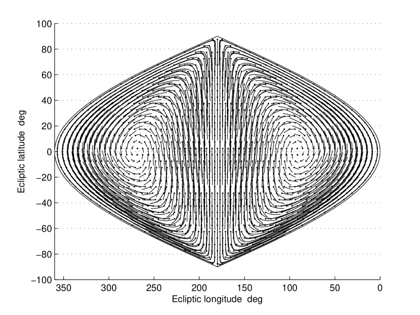
Figure 1: The magnetic vector spherical harmonic ${\bf H}_{1}^{-1}$.

2.2 A direct solution on a laptop

The most important advantage of the spherical harmonics is that they are orthogonal on the unit sphere in the space of continuous functions, or nearly orthogonal when discretized on a large set of uniformly distributed points. In the latter case, the deviation from orthogonality is negligibly small for a sufficiently large number of grid stars ($\gtrsim 10^{4}$) of uniform density on the sky. The degree of uniformity and the number of grid stars should be higher if the higher order harmonics are to be used in the direct global solution. Normally, the lower orders of spherical harmonics are of interest, where the largest correlated errors emerge. Therefore, the series in Eq. 3 can be truncated in the new condition equations for the fitting coefficients $S_{j}$, $M_{j}$, and $Q_{j}$. The solution for a subset of model terms is exact if the terms are orthogonal. In practice, the degree of orthogonality should be verified for a given distribution of stars and weights (in a weighted LS). Rearranging the discretized spherical harmonics for the three types of astrometric unknowns as columns of a design matrix, the unknown coefficients and the right-hand side data as column vectors, the LS problem can be written in this compact matrix form:

$$\left[{\bf V}_{s}\,{\bf V}_{\mu}\,{\bf U}_{\varpi}\right]\;\left[\begin{array}[]{c}{\bf S}\\ {\bf M}\\ {\bf Q}\end{array}\right]={\bf y}$$ (6)

The length of the design matrix is still very large in this setup, because it includes all the observations of grid stars. For JMAPS, it is about 144 million for 1 million grid stars. The width of the design matrix, on the other hand, is defined by how many spherical harmonic terms we want to solve for. Indeed, a sufficiently accurate solution can be obtained for any subset of spherical harmonics, as long as the columns of the design matrix are nearly orthogonal. This is verified by computing the correlation coefficients of the covariance matrix. They should all be small, e.g., less than 0.01 in absolute value. If this is the case, including more terms in the design matrix will not change the solution for $S_{j}$, $M_{j}$, and $Q_{j}$ significantly. The number of unknowns can be made comfortably small for a given computer. We found, for example, that a global solution can be obtained within 1 hour for 400 unknowns on a regular laptop computer.

Even with a limited number of unknowns, the design matrix is too large to be handled in fast memory without swapping with disk. However, there is no need to keep the entire matrix in memory if the observations are sorted by time. If the design matrix ${\bf D}=\left[{\bf V}_{s}\,{\bf V}_{\mu}\,{\bf U}_{\varpi}\right]$ is divided into a number of blocks ${\bf D}_{j}$ in the vertical dimension (not necessarily of the same length), the normal matrix is the sum of the normal sub-matrices, ${\bf D}^{T}{\bf D}=\sum_{j}{\bf D}_{j}^{T}{\bf D}_{j}$. The accumulated normal matrix can be easily inverted due to its relatively small size, resulting in the covariance matrix, ${\bf Cov}=\left({\bf D}^{T}{\bf D}\right)^{-1}$. The off-diagonal elements of ${\bf Cov}$ should be small due to the near-orthogonality of the model terms, unless some additional global parameters are included. The diagonal elements are the variances of unit weight of the coefficients of spherical harmonics $S_{j}$, $M_{j}$, and $Q_{j}$. If the observations are weighted by the expected standard deviation of measurement error, the variances are the squares of the standard errors carried by the corresponding spherical harmonics. The total mission-average variance is approximately the sum of the variances of the complete set of harmonics for each of the 5 astrometric parameters. Since we obtain the variances for a limited set of harmonics, the total mission-average error can not be inferred from this computation. However, the uncertainty of specific harmonic components is accurately computed.

3 Results and Discussion

JMAPS is a pointing astrometric telescope with a single viewing direction. Without the ability of Hipparcos to simultaneously observe stars that are far apart on the sky, the required rigidity of the reference system and the accuracy of astrometric parameters is achieved through measuring a number of carefully selected ICRF and radio-mute quasars and other extragalactic objects. These objects provide absolute constraints on positions (using the ICRF coordinates of superior accuracy), parallaxes and proper motions, which are negligibly small because of the extreme remoteness. The entire sky is observed with a 4-fold overlap. Astrometric observations are normally made around the great circle perpendicular to the sun direction. Some 72 observations per object are expected to be collected in three years. For the simulations described in this paper, we used a catalog of 44 ICRF quasars and 80 compact extragalactic sources (QSO), which are not in the ICRF. All these reference quasars are brighter than magnitude 15. Only a subset of all observable stars, usually between 1 and 2 million strong, is used in the direct global solution.

The attitude unknowns are represented by three parameters for each frame, viz., the translations along the axes of the detector and rotation around the boresight vector. These unknowns are eliminated frame by frame, reducing the number of conditions by three. The instrument calibration unknowns are represented in these simulations by sets of up to 28 Zernike polynomials of field coordinates, separately for either coordinate in the detector plane. The first Zernike polynomials, which are constant, are excluded to avoid deficiency of rank, because they are indistinguishable from the attitude translations. In our simplified simulations, the calibration parameters are assumed to be constant within calibration blocks of equal length. Usually, blocks of 92 or 96 consecutive frames are used, corresponding to roughly 50 min of uninterrupted observations. As soon as a complete calibration block is collected, the QR factorization is applied, and the remaining astrometric equations are pre-multiplied with ${\bf Q}^{T}$, as well as the right-hand side. The number of condition equations is further reduced by $2\,N_{Z}$ for each calibration block, with $N_{Z}$ being the number of calibration parameters. This algorithm allows us to include a set of global parameters, which do not vary with time, such as the PPN $\gamma$-parameter. The accuracy or precision of global parameters can be reliably estimated, because they are mostly correlated with the low-order components. The number of vector spherical unknowns is $2(N_{V}+1)^{2}-2$, where $N_{V}$ is the limiting degree, and the number of scalar spherical harmonics (for parallax) is $(N_{V}+1)^{2}$.

3.1 Accidental errors

The statistical properties of accidental correlated errors are defined by the global covariance matrix of the coefficients of spherical harmonics. The diagonal of the covariance matrix at $N_{V}=7$ includes 126 vector spherical harmonic coefficients for positions and proper motions each and 64 scalar spherical harmonic coefficients for parallax. The square roots of the portions of the diagonal corresponding to each astrometric parameter are the standard deviations of error of unit weight, represented by a particular harmonic. For example, the standard deviation of the parallax zero-point error is the the standard deviation of the first spherical harmonic coefficient multiplied by the weighted average single measurement precision of stars and quasars. Figs. 2 a and b show the standard deviations of harmonic errors of proper motions and parallax, respectively, obtained from a typical simulation of JMAPS mission. Generally, we find that the correlated errors in all three parameters fairly rapidly decline with the degree of spherical harmonic. To use an analogy from spectroscopy, in that sense, the spectrum of accidental errors is “red”. There are some obvious “spectral lines”, however, which are caused by the observing pattern and the distribution of reference quasars on the sky.

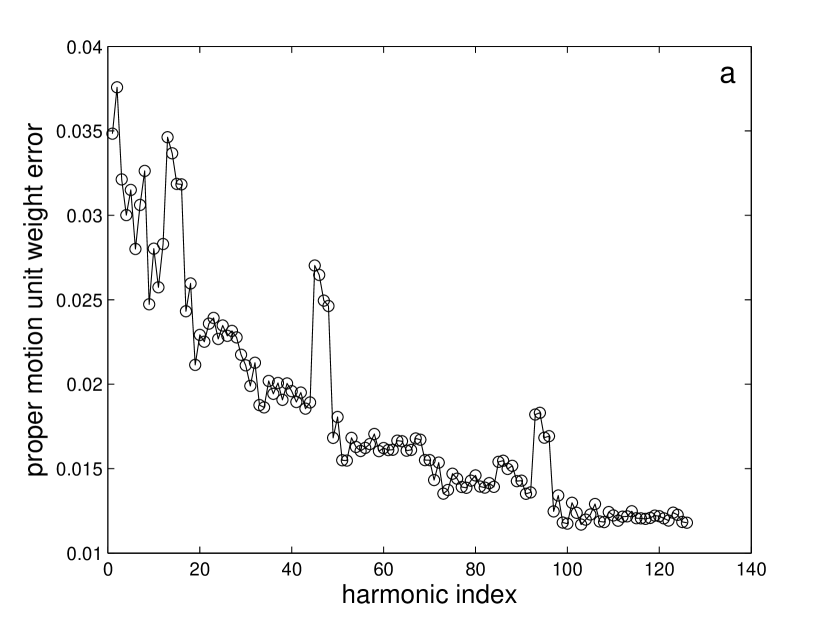
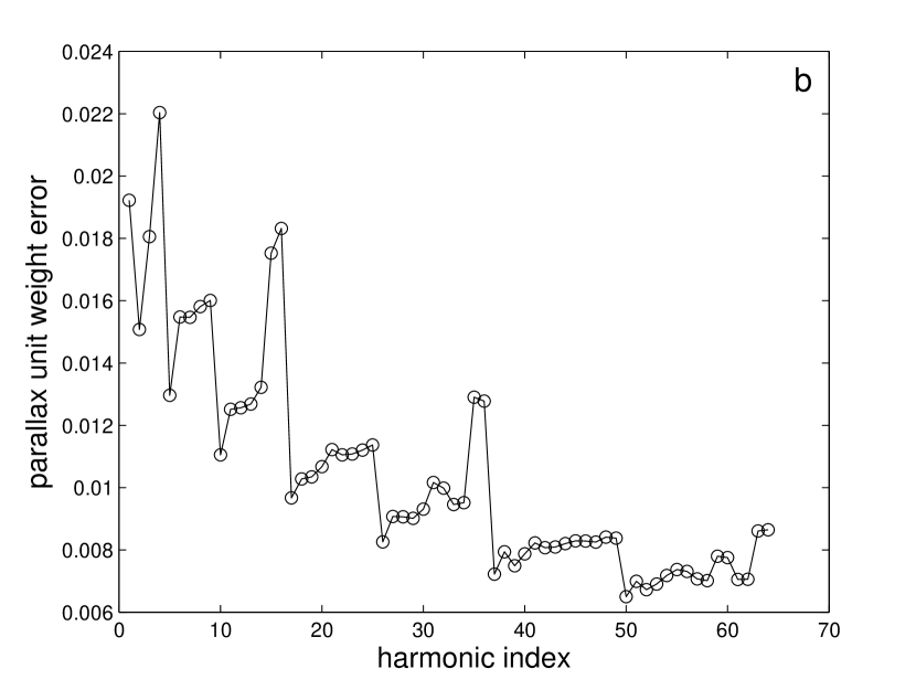
Figure 2: Standard deviations of the coefficients of spherical harmonics representing accidental error in a) proper motions, and b) parallax. The errors are normalized to unit weight.

We find that the distribution of accidental error becomes flatter with a significantly larger number of grid quasars. The relative height of the “spectral lines” depends on the distribution of grid quasars on the sky and the composition of the calibration model. Large holes in the distribution of quasars cause considerable degradation of the overall performance. Using the near-orthogonality of the discretized spherical function, the variance of accidental error of, e.g., proper motion at a given point $(\lambda,\beta)$ can be estimated as

$${\rm var}[{\bf\mu}(\lambda,\beta)]\simeq\sum_{j}{\rm var}\left[M_{j}\right]\|{\bf V}_{j}(\lambda,\beta)\|^{2}=\sum_{j}C_{\mu,jj}\|{\bf V}_{j}(\lambda,\beta)\|^{2}$$ (7)

where ${\bf C}_{\mu}$ is the corresponding part of the covariance matrix. Since this decomposition is limited to a finite set of spherical functions, only a lower bound of the total error can be obtained. Still, the distribution of the error carried by the lower-order harmonics is very informative. For example, one can estimate the degree of inhomogeneity of the correlated error on the celestial sphere, which can be significant for JMAPS. Fig. 3 depicts the distribution of the standard deviation of the total accidental error of parallax, which is contained in the first 64 scalar spherical harmonics. The plot is rotated into the Galactic coordinate system to emphasize the impact of the zone of avoidance around the Galactic plane where quasars brighter than 15 mag can not be found. The quasars, which were used to constrain the global solution for parallax, are shown as black dots. The build-up of error in the areas devoid of grid quasars is quite obvious. As a way of improving the overall mission performance, fainter quasars should be found near the Galactic plane and included in the grid.

Figure 3: Sky distribution of the standard deviation of parallax unit weight error for a simulated JMAPS mission. The reference quasars used to constrain the parallax solution are marked with black dots.

It should be noted that the distribution in Fig. 3 corresponds to the expectancy of the spatially correlated error rather than to the outcome of a single mission. In other words, it shows what would emerge if the same mission is simulated many times with random noise in the input data, and the sample variance of the resulting errors is computed at each point. A single random realization of correlated error can be computed by

$$\delta{\bf\mu}(\lambda,\beta)=\left({\bf C}_{\mu}^{\frac{1}{2}}{\bf r}\right)^{T}{\bf V}(\lambda,\beta)$$ (8)

with ${\bf C}_{\mu}^{\frac{1}{2}}$ being the unique positive definite matrix square root of ${\bf C}_{\mu}$, ${\bf r}$ a random vector drawn from ${\cal N}(0,1/N_{V})$ of $N_{V}$ elements, and ${\bf V}(\lambda,\beta)$ the column vector of the values ${\bf V}_{j}(\lambda,\beta)$. These transformations are performed separately for each coordinate direction for the vector-valued parameters (position and proper motion).

3.2 Systematic errors

Systematic errors of global solutions are much harder to predict and analyze, because there are multiple sources of such errors, which are rarely known beforehand. Slowly varying perturbations of observational data, caused by external circumstances, are of special interest, as they can bring about smooth, large-scale errors. The orientation of the astrometric satellite with respect to the sun direction is one of the conceivable sources of systematic error. The angle between the sun direction, which is confined to the ecliptic plane, and the viewing direction changes in a predetermined way, because the entire celestial sphere should be observed as uniformly as possible. The thermal flow inevitably changes inside the telescope, resulting in slowly varying instrument parameters, e.g., the effective focal length or the basic angle for Gaia. If these variations are correlated with the celestial coordinates, there is no averaging out of the perturbation, and the error can propagate into the final catalog. In many cases, such specific physical influences can not be accurately modeled or predicted. A more general modeling approach can be exploited, where a certain perturbation is represented as a set of basis functions. For example, a systematic variation of the basic angle can be represented as a Fourier series of the sun angle, and each of the Fourier terms can be simulated separately. The previous studies for Hipparcos and SIM indicate that many of such elementary perturbations are benign, in that they cause a relatively small error. There are, however, some particularly dangerous perturbations, which may propagate into the final catalog with considerable magnification. Such harmful systematic effects should be identified and mitigated, if possible. This requires numerous mission simulations with different initial data, which may not be feasible for the extremely computer-intensive solutions for millions of individual grid objects. The proposed technique is fast enough to be used for massive simulations of slowly varying systematic perturbations, when the emerging astrometric error is confined to the lower degrees of spherical harmonics.

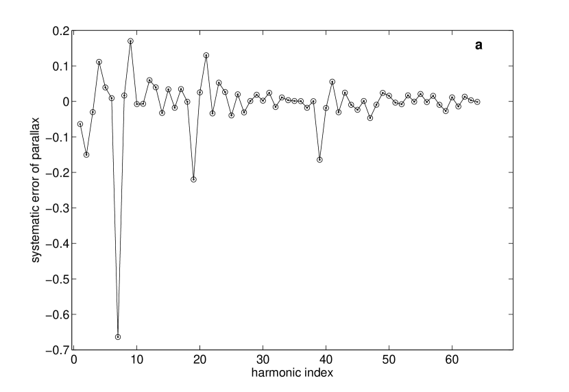
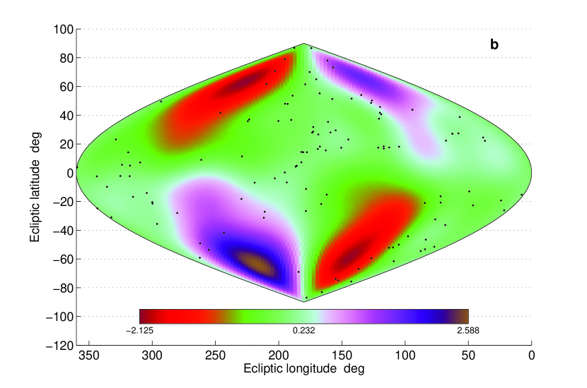
Figure 4: Systematic error of JMAPS parallax resulting from a constant perturbation of the differential scale by 1 mas at the edge of the field of view: a) in the coefficients of the first 64 spherical harmonics; b) on the sky. All values are in mas.

Figure 4 shows the results of a specific simulation for JMAPS, where a perturbation in the field-dependent calibration parameter $Z_{2}$ was injected in the observational data, but not fitted out in the global solution. The term $Z_{2}$ (second Zernike polynomial) corresponds to the differential scale of the instrument. The magnitude of the perturbation was normalized to 1 mas at the edge of the field of view. The simulated observations ($X$ and $Y$ measurements) were free of random noise, to see more clearly the emerging pattern of the correlated error. The absolute error in the coefficients of 64 lower-order spherical harmonics is depicted in Fig. 4a. The spectrum of the error is dominated by the harmonic number 7 (which is $U_{2}^{0}$), followed by harmonic 19 ($U_{4}^{-2}$) and so on. The total absolute error of parallax at a given point is the sum of all spherical harmonic errors. The total error in the first 64 harmonics is depicted in Fig. 4b. It shows that the simulated perturbation is one of the harmful errors for JMAPS, because it compounds to a perturbation of up to 2.6 mas in some parts of the sky, which is larger than the initial magnitude. Clearly, the distribution of constraining quasars, shown with black dots, plays a major role in the propagation of this systematic error, which compounds to larger values in the areas where the quasars are few. If the calibration term $Z_{2}$ is included in the set of fitting parameters in the global solution, the emerging error is zero in the absence of random noise.

4 Conclusions

We developed a method to investigate the properties of very large astrometric solutions, which involve unknown parameters for millions of celestial sources, as well as millions of nuisance unknowns. The method is based on a stepwise elimination of the attitude and calibration unknowns and the replacement of individual astrometric corrections with their expansions in orthogonal spherical functions of celestial coordinates. This approach works well for the JMAPS and SIM missions and could potentially be useful for Hipparcos and Gaia. However, demonstrating the applicability of the method to Hipparcos-like missions would require considerable adjustments, mostly related to the dynamic character of attitude parameters, which is beyond the scope of this paper. In particular, fitting a set of dynamic parameters for each extended interval of uninterrupted rotation may render the proposed technique of QR-elimination of the attitude unknowns impractical. An additional complication arises for Gaia, where each of the multiple CCDs in the focal plane requires a separate set of calibration parameters. The pointing, or step-stare mode of operation of JMAPS makes it best-suited for the proposed global solution technique with block-wise elimination of attitude and calibration parameters, so that complete analysis for realistic sky coverages and observing schedules can be performed for billions of condition equations. The propagation of zonal and correlated errors of both accidental and systematic origin can be successfully computed using this method. When the number of expansion terms is appropriately small, full mission solutions can be obtained using regular computers within a few hours with more than a hundred million unknowns. Some applications of the spherical harmonic solution to the JMAPS mission are described.

References

- Bucciarelli et al. (1991) Bucciarelli, B., et al. 1991, Adv. Space Res., 11, 79
- ESA (1997) ESA, 1997, The Hipparcos Catalogue, ESA SP-1200, Vol. 1-17
- Gaume (2011) Gaume, R. 2011, EAS Publ. Ser., 45, 143
- Hoyer et al. (1981) Hoyer, P., et al. 1981, A&A, 101, 228
- Lammers et al. (2010) Lammers, U., et al. 2010, ASP Conf. Ser., 434, 309
- Lim et al. (2010) Lim, T.W., Tasker, F.A., & DeLaHunt, P.G. 2010, The Joint Milli-Arcsecond Pathfinder Survey (JMAPS) Instrument Fine Attitude Determination Approach, Proc. 33rd AAS GNC Conf., AAS 10-031
- Makarov (1992) Makarov, V.V. 1992, Soviet Astronomy Lett., 18, 252
- Makarov et al. (1995) Makarov, V.V., Høg, E., & Lindegren, L. 1995, Experimental Astronomy, 3, 211
- Makarov et al. (1998) Makarov, V.V. 1998, A&A, 340, 309
- Makarov & Milman (2005) Makarov, V.V., Milman, M. 2005, PASP, 117, 757
- Makarov & Murphy (2007) Makarov, V.V., Murphy, D.W. 2007, AJ, 134, 367
- Mignard & Frœschlé (2000) Mignard, F., Frœschlé, M. 2000, A&A, 354, 732
- O’Mullane et al. (2011) O’Mullane, W., et al. 2011, Experimental Astronomy, 31, 215
- Perryman (2003) Perryman, M.A.C. 1998, in GAIA Spectroscopy: Science and Technology, ed. U.Munari, ASP Conf. Proc 298, 3
- Unwin et al. (2008) Unwin, S., et al. 2008, PASP, 120, 38
- van Leeuwen (2007) van Leeuwen, F. 2007, A&A, 474, 653
- von der Heide (1977) von der Heide, K. 1977, A&A, 61, 553
- Zacharias & Dorland (2006) Zacharias, N., Dorland, B. 2006, PASP, 118, 1419