The role of axisymmetric flow configuration in the estimation of the analogue surface gravity and related Hawking like temperature

Abstract

For axially symmetric flow of dissipationless inhomogeneous fluid onto a non rotating astrophysical black hole under the influence of a generalized pseudo-Schwarzschild gravitational potential, we investigate the influence of the background flow configuration on determining the salient features of the corresponding acoustic geometry. The acoustic horizon for the aforementioned flow structure has been located and the corresponding acoustic surface gravity $\kappa$ as well as the associated analogue Hawking temperature $T_{\rm AH}$ has been calculated analytically. The dependence of $\kappa$ on the flow geometry as well as on the nature of the back ground black hole space time (manifested through the nature of the pseudo-Schwarzschild potential used) has been discussed. Dependence of the value of $\kappa$ on various initial boundary conditions governing the dynamic and the thermodynamic properties of the background fluid flow has also been studied.

1 Introduction

Contemporary works in the field of analogue gravity phenomena have attracted significant attention in the community [1, 2, 3, 4]. Proper equivalence has been established between the physics of the propagating acoustic (and acoustic type) perturbations embedded in an inhomogeneous dynamical fluid system, and some kinematic features of the general theory of relativity. Such formalism has opened up the possibility of simulating various important features of the black hole space time within the laboratory set up.

Conventional works in this field, however, concentrates on the physical systems for which gravity like effects are realized as emergent phenomena. Such systems do not usually contain any source that produces active gravitational field in any form. In recent years, though, attempts have been made to study the analogue effects in strong gravity environment [5, 6, 7, 8, 9, 10, 11, 12, 13]. The uniqueness of such systems lies in the fact that those are the only analogue models studied so far that simultaneously contain both kind of horizons, the gravitational as well as the acoustic - allowing one to go for a close comparison between the actual and the analogue Hawking effect.

Till date, analogue effects in the axisymmetrically accreting black hole systems has been studied for the flow structure assumed to be in hydrostatic equilibrium in the vertical direction. Two other configurations for the axially symmetric black hole accretion are also possible. Acccretion flow in conical equilibrium [14] and ‘flat disk’ kind of flow with constant flow thickness have also been studied in the literature (see, e.g., [15] for detail review). For pseudo-Schwarzschild gravitational potential , the aforementioned three different flow structures have quite recently been studied in great detail ([18]). to reveal various critical phenomena and stability properties of such flows.

In our present work, we study the analogue effects in accreting black hole systems under the influence of pseudo-Schwarzschild potentials for three different flow configurations - flow in conical and in vertical equilibrium and for constant thickness (height) flow. The main motivation behind this work is to study the dependence of the salient features of the acoustic geometry on the background geometry realized through the aforementioned three different flow configurations. To accomplish such task, we will calculate the acoustic surface gravity for same set of accretion parameters but for all possible flow configurations in a pseudo-Schwarzschild potentials.

2 Acoustic surface gravity for classical analogue systems

Classical analogue gravity systems (alternatively, the classical ‘black hole analogues‘) are fluid dynamical analogue of black holes in general relativity. Such analogue may occur when a small linear perturbation propagates through a dissipation less inhomogeneous barotropic transonic fluid at finite temperature. The corresponding acoustic metric, which specifies the geometry in which the perturbation propagates, may be constructed in terms of the flow variables defining the unperturbed background continuum. The transonic surface acts as acoustic horizon - a null hypersurface with acoustic null geodesics, the phonons, as its generators. The acoustic black hole horizon, which resembles the black hole event horizons in many ways, may form at the regular transonic point of the fluid, whereas an acoustic white hole horizon may be formed at the hypersurface where the fluid makes a discontinuous sonic transition, e.g., through a stationary shock [19, 8].

In his pioneering work Unruh [20] introduced the concept of acoustic geometry inside a supersonic fluid and demonstrated that an analogue surface gravity $\kappa$ may be associated with an acoustic black hole type event horizon, and one of the most interesting aspects of the acoustic horizon is to emit the Hawking type radiation of thermal phonons. Such acoustic Hawking radiation may be characterized by a analogue Hawking temperature $T_{\rm AH}=\frac{{\hbar}{\kappa}}{2{\pi}}$. In Unruh’s original approach, the acoustic surface gravity could be associated with the component of the bulk velocity of the flow normal to the acoustic horizon $u_{\perp}$ and the speed of propagation of the acoustic perturbation $c_{s}$ as

$$\kappa~{}{\propto}\left(\frac{1}{c_{s}}\frac{{\partial}{u_{\perp}^{2}}}{{\partial}{\eta}}\right)_{r_{h}}$$ (2.1)

where $\frac{\partial}{\partial{\eta}}=\eta^{\mu}{\partial}_{\mu}$ represents the space derivative taken along the normal to the acoustic horizon, and every quantities in the eq. (2.1) has been evaluated at the location of the acoustic horizon $r_{h}$.

In eq. (2.1), however, the sound speed was assumed to be a position independent constant. Unruh’s work was followed by several other important contributions ([21, 22, 23, 24] , to name a few) Visser [23] implemented the additional contribution due to the position dependent sound speed and obtained a modified expression for the surface gravity

$$\kappa~{}{\propto}\left[c_{s}\frac{\partial}{\partial{\eta}}\left(c_{s}-u_{\perp}\right)\right]_{r_{h}}$$ (2.2)

The acoustic horizon is a surface defined by the equation [23]

$$u_{\perp}^{2}-c_{s}^{2}=0$$ (2.3)

for the stationary background flow configuration. Equation (2.3) basically states that the acoustic horizons is a transonic surface. The supersonic region of a transonic flow defines the acoustic ergo region.

The concept of acoustic geometry has been extended to a relativistic fluid flow in a general background space time [26]. For an ideal barotropic fluid, the relativistic Euler equation and the equation of continuity obtained from the energy momentum conservation can be linearized in order to obtain the wave equation for the propagating perturbation in analogue curved space time with the corresponding acoustic metric. The generalized form of the acoustic surface gravity turns out to be

$$\kappa=\left|\frac{\sqrt{{\chi^{\mu}}{\chi_{\mu}}}}{\left(1-{c_{s}}^{2}\right)}\frac{\partial}{\partial{\eta}}\left(u_{\perp}-{c_{s}}\right)\right|_{r_{h}}$$ (2.4)

where $\chi^{\mu}$ is the Killing field which is null on the corresponding acoustic horizon. The algebraic expression corresponding to the $\sqrt{\chi^{\mu}{\chi_{\mu}}}$ may thus be evaluated once the background stationary metric governing the fluid flow as well as the propagation of the perturbation in a specified geometry with well posed boundary conditions are realized. It is worth mentioning that the generalized form for $\kappa$ as defined in eq. (2.4) can further be reduced to its Newtonian/semi Newtonian counterpart depending on the nature of the gravitational potential describing the background fluid motion.

3 Acoustic surface gravity for axisymmetric black hole accretion

From (2.2) and (2.4) it is clear that, in order to find the acoustic surface gravity $\kappa$ for the Newtonian as well as for the general relativistic acoustic geometry, it is sufficient to calculate the location $r_{h}$ of the acoustic horizon, the sound speed $c_{s}$ of the small linear perturbation and its normal space gradient $dc_{s}/d{\eta}$, as well as the the normal (to the acoustic horizon) component of the flow velocity $u_{\perp}$ and its normal space gradient $du_{\perp}/d{\eta}$, evaluated on the acoustic horizon.

For transonic accretion onto astrophysical black hole, one thus needs to consider the Euler equation and the equation of continuity for a specific symmetry of the problem. The Euler and the continuity equation may then be linearized (for a general linearization scheme and its application to the study of axisymmetric black hole accretion for three different flow geometries see [18]) in order to construct the corresponding acoustic metric to specify the relevant acoustic geometry. The structure of the stationary background fluid flow may be provided by the stationary solution of the Euler and the continuity equations. For a certain set of values of the initial conditions describing the transonic accretion flow governed by certain barotropic equation of state, it may be possible to find the location of the saddle type transonic point, which is identical to the acoustic black hole horizon (see [7, 26, 8, 10] ). The quantities $\left[u_{\perp},c_{s},du_{\perp}/dr,dc_{s}/dr\right]_{r_{\rm transonic}}$ subject to a gravitational field which governs the accretion, may then be evaluated to estimate the acoustic surface gravity using eq. (2.4). The quantity $\sqrt{\chi^{\mu}{\chi_{\mu}}}$ evaluated at the acoustic horizon is a function of ${r_{h}}={r_{\rm transonic}}$ (as will be demonstrated in subsequent paragraphs) depending on initial conditions.

In general, we consider the equatorial slice of the axisymmetric gravitating accretion of hydrodynamic fluid onto non rotating black holes. The gravitational field of the black hole is assumed to be described by certain pseudo-Schwarzschild potentials. The Schwarzschild radius $r_{g}=2GM_{\rm BH}/c^{2}$ is used to scale the radial distance, whereas all velocities involved are scaled by the velocity of light in vacuum $c$, $G=c=1$ has been used. Accretion is assumed to possess finite radial velocity $u$ commonly known as the ‘advective velocity’ in the accretion literature. Considering $v$ to be the magnitude of the three velocity, $u$ is the component of three velocity perpendicular to the set of timelike hypersurfaces $\left\{\Sigma_{v}\right\}$ defined by $v^{2}={\rm constant}$. The advective velocity $u$ is thus perpendicular to the acoustic horizon and hence $u$ is identical with $u_{\perp}$. Hereafter we drop the subscript $\perp$ in $u_{\perp}$ and simply use $u$ instead.

The low angular momentum sub-Keplerian advective inviscid flow will be considered where the specific flow angular momentum $\lambda$ will be assumed to be a position independent constant. Viscous transport of angular momentum will not be taken into account since close to the black hole, the infall time scale for the highly supersonic flow is rather small compared to the corresponding viscous time scale (see, e.g., [17, 27, 28] and references therein for further detail). Also for advective accretion, large radial velocity at a larger distances are the consequence of the small rotational energy of the flow [29, 30, 31] . The corresponding angular velocity $\Omega$ may be defined as ([28] and references therein)

$$\Omega==-\frac{g_{t\phi}+\lambda{g}_{tt}}{{g_{\phi{\phi}}+\lambda{g}_{t{\phi}}}}$$ (3.1)

where $g_{ij}$ are the metric components.

The corresponding surface gravity $\kappa$ can now be expressed as

$$\kappa=\left|\sqrt{\frac{\chi^{\mu}{\chi_{\mu}}}{-g_{rr}}}\frac{1}{1-c_{s}^{2}}\left[\frac{d}{d{r}}\left(u-{c_{s}}\right)\right]\right|_{r_{h}}$$ (3.2)

where $\chi^{\mu}=\xi^{\mu}+\Omega{\varsigma^{\mu}}$ and the Killing vectors $\xi^{\mu}$ and $\varsigma^{\mu}$ are the generators of the temporal and the axial symmetry group. The norm of the Killing vector $\chi_{\mu}$ may be computed as

$$\sqrt{\chi^{\mu}{\chi_{\mu}}}=\left(g_{tt}+2\Omega{g_{t\phi}}+\Omega^{2}{g_{\phi\phi}}\right)^{\frac{1}{2}}=\frac{{\Sigma}{\Lambda}}{g_{\phi{\phi}}+\lambda{g_{t\phi}}}$$ (3.3)

where

$$\Sigma^{2}=g^{2}_{t{\phi}}-g_{tt}g_{\phi{\phi}}$$ (3.4)

$$\Lambda^{2}=\left(g_{tt}+2\lambda{g_{t\phi}}+\lambda^{2}{g_{\phi\phi}}\right)$$

In the Newtonian limit

$$g_{tt}=1+2\phi,~{}g_{{\phi}{\phi}}=-r^{2},~{}g_{rr}=-1,~{}g_{t\phi}=0$$ (3.5)

where $\Phi$ is the pseudo potential. Hence the acoustic gravity for axisymmetric black hole accretion under the influence of the pseudo-Schwarzscild potential becomes

$$\kappa=\left|\sqrt{\left(1+\Phi\right)\left(1-\frac{\lambda^{2}}{r^{2}}-2\Phi\frac{\lambda^{2}}{r^{2}}\right)}\left(\frac{1}{1-c_{s}^{2}}\left[\frac{du}{dr}-\frac{dc_{s}}{dr}\right]\right)\right|_{r_{h}}$$ (3.6)

Our main task now boils down to the evaluation of $c_{s}$, $dc_{s}/dr$ and $du/dr$ on the acoustic horizon for the pseudo-Schwarzschild axisymmetric black hole accretion in three different flow configurations as mentioned in previous sections.

4 Generalized transonic accretion in three different flow geometries

The governing equations describing the dynamics of axially symmetric pseudo-Schwarzschild inviscid hydrodynamics accretion are the equation for the conservation of linear momentum (the Euler equation):

$$\frac{{\partial}}{{\partial}t}u(r,t)+u(r,t)\frac{{\partial}}{{\partial}r}u(r,t)+\frac{1}{\rho(r,t)}\frac{{\partial}p(r,t)}{{\partial}r}-\frac{\lambda^{2}}{r^{3}}+\Phi^{\prime}=0$$ (4.1)

where $u,\rho$ and $p$, being the dynamical flow velocity, the fluid density and the pressure, respectively, are functions of both $r$ and $t$. $\Phi$ may be taken as any one of the following four pseudo-Schwarzschild potentials:

$$\Phi_{1} = -\frac{1}{2(r-1)},$$ (4.2a)

$$\Phi_{2} = -\frac{1}{2r}\left[1-\frac{3}{2r}+12{\left(\frac{1}{2r}\right)}^{2}\right],$$ (4.2b)

$$\Phi_{3} = -1+{\left(1-\frac{1}{r}\right)}^{\frac{1}{2}},$$ (4.2c)

$$\Phi_{4} = \frac{1}{2}{\rm ln}{\left(1-\frac{1}{r}\right)}$$ (4.2d)

The potential $\Phi_{1}$ and $\Phi_{2}$ have been introduced in [32] and [33] , respectively, whereas $\Phi_{3}$ and $\Phi_{4}$ have been introduced in [16] .

The mass conservation equation (the continuity equation) can be written as:

$$\frac{{\partial}}{{\partial}t}\rho(r,t)+\frac{\partial}{{\partial}{r}}\left[\rho(r,t){u(r,t)rH}\right]=0$$ (4.3)

The quantity $H$ is the flow thickness which is different in three different flow configurations. For the simplest possible flow configuration, the flow thickness (i.e., the disc height) is constant, and hence $H$ is not a function of the radial distance. In its next variant, the flow can have a conical structure (see [14] ) where $H$ is directly proportional to the radial distance as $H=Ar$, where the geometric constant $A$ depends on the solid angle subtended by the flow. For hydrostatic equilibrium in vertical direction [34, 35], the flow thickness can have a rather complex dependence on the radial distance and on the local adiabatic sound speed [17, 27] defined as $c_{s}=\sqrt{\left(\frac{\partial{p}}{\partial{\rho}}\right)}$. The barotropic equation of state will in general be used to describe the accretion flow in this work. A polytropic equation of state $p=K{\rho}^{\gamma}$ will be used, whereas the isothermal flow will be governed by the equation $p=\frac{\rho{\kappa_{B}}T}{{\mu}m_{H}}$. The quantities $K,\gamma,\kappa_{B},T,\mu$ and $m_{H}$ are the entropy per particle, the Boltzmann constant, the isothermal flow temperature, the reduced mass and the mass of the Hydrogen atom, respectively. With the help of the equation of states, and the specified radial dependence of the flow thickness, we can find stationary solutions of the Euler and the continuity equations and draw the Mach number versus the radial distance phase portrait for the integral flow solutions to obtain the detail information about the location of the acoustic horizon as well as the horizon related quantities.

4.1 Polytropic Accretion

For polytropic equation of state, the integral solution of the stationary part of the Euler equation provides the energy first integral of motion of the following form:

$${\cal E}=\frac{u^{2}}{2}+\frac{c_{s}^{2}}{\gamma-1}+\frac{\lambda^{2}}{2r^{2}}+\Phi$$ (4.4)

The conserved specific energy ${\cal E}$ does not depend on the flow configuration for obvious reason. Since $r$ dependence of $H$ varies for different flow geometries, the integral solution of the continuity equation, which is another first integral of motion and is referred to as the mass accretion rate, will be different for three different accretion configurations. Expressions for the mass accretion rate can be obtained as:

$${\dot{M}}_{\rm CH}=\rho{u}rH_{c}$$ (4.5a)

$${\dot{M}}_{\rm CM}=\Theta{\rho}ur^{2}$$ (4.5b)

$${\dot{M}}_{\rm VE}=\sqrt{\frac{1}{\gamma}}uc_{s}{\rho}r^{\frac{3}{2}}\left(\Phi^{\prime}\right)^{-\frac{1}{2}}$$ (4.5c)

where the subscript CH,CM and VE stands for the flow with constant height (CH), in conical model (CM), and in vertical equilibrium (VE), and implies that the respective algebraic equations are to be solved to obtain the critical point for the corresponding flow geometries. The quantity $H_{c}$ is the constant disc height and $\Theta$ is the solid angle sustained by the flow. The mass accretion rate for flow in vertical equilibrium not only depends on the matter geometry (through the radial dependence of $H$), but also the information about the space time geometry is encrypted in ${\dot{M}}_{\rm VE}$ through the explicit appearance of the derivative of the pseudo-Schwarzschild potential. One defines the entropy accretion rate as ([14, 36]):

$${\dot{\cal M}}={\dot{M}}\gamma^{\frac{1}{\gamma-1}}K^{\frac{1}{\gamma-1}}$$ (4.6)

Substitution of ${\dot{M}}$ from eq. (4.5) in the above equation provides the expression for ${\dot{\cal M}}$ in terms of the adiabatic sound speed, radial distance, and the dynamical flow velocity. The space gradient of the sound speed as well as the dynamical velocity for various flow geometries can be obtained by differentiating eq. (4.4) and eq. (4.6):

$$\left(\frac{dc_{s}}{dr}\right)_{\rm CH} = (1-\gamma)\frac{c_{s}}{u}\left(\frac{1}{2}\frac{du}{dr}+\frac{u}{2r}\right)$$ (4.7a)

$$\left(\frac{dc_{s}}{dr}\right)_{\rm CM} = (1-\gamma)\frac{c_{s}}{u}\left(\frac{1}{2}\frac{du}{dr}+\frac{u}{r}\right)$$ (4.7b)

$$\left(\frac{dc_{s}}{dr}\right)_{\rm VE} = \left(\frac{1-\gamma}{1+\gamma}\right)\frac{c_{s}}{u}\left[\frac{du}{dr}+\frac{u}{2}\left(\frac{3}{r}-\frac{\Phi^{\prime\prime}(r)}{\Phi^{\prime}(r)}\right)\right]$$ (4.7c)

$$\left(\frac{du}{dr}\right)_{\rm CH} = \frac{u\left(\frac{c_{s}^{2}}{r}+\frac{\lambda^{2}}{r^{3}}-\Phi^{\prime}(r)\right)}{\left(u^{2}-c_{s}^{2}\right)}$$ (4.8a)

$$\left(\frac{du}{dr}\right)_{\rm CM} = \frac{u\left(\frac{2c_{s}^{2}}{r}+\frac{\lambda^{2}}{r^{3}}-\Phi^{\prime}(r)\right)}{\left(u^{2}-c_{s}^{2}\right)}$$ (4.8b)

$$\left(\frac{du}{dr}\right)_{\rm VE} = \frac{u\left[\frac{c_{s}^{2}}{(1+\gamma)}\left(\frac{3}{r}-\frac{\Phi^{\prime\prime}(r)}{\Phi^{\prime}(r)}\right)+\frac{\lambda^{2}}{r^{3}}-\Phi^{\prime}(r)\right]}{\left(u^{2}-\frac{2}{1+\gamma}c_{s}^{2}\right)}$$ (4.8c)

The critical point conditions may be obtained by simultaneously making the numerator and the denominator of eq. (4.8) vanish, and the aforementioned critical point conditions may thus be expressed as:

$$\left(u\right)_{r_{c}}=\left({c_{s}}\right)_{rc}$$ (4.9a)

$$\left({c_{s}}\right)_{r_{c}}=\sqrt{r_{c}\Phi^{\prime}(r_{c})-\frac{\lambda^{2}}{r_{c}^{2}}}$$ (4.9b)

$$\left(u\right)_{r_{c}}=\left({c_{s}}\right)_{rc}$$ (4.10a)

$$\left({c_{s}}\right)_{r_{c}}=\sqrt{\frac{r_{c}\Phi^{\prime}(r_{c})}{2}-\frac{\lambda^{2}}{2r_{c}^{2}}}$$ (4.10b)

$$\left(u\right)_{r_{c}}=\sqrt{\frac{2}{\gamma+1}}\left({c_{s}}\right)_{rc}$$ (4.11a)

$$\left({c_{s}}\right)_{rc}=\sqrt{(\gamma+1)\frac{\left[\Phi^{\prime}(r_{c})-\frac{\lambda^{2}}{r_{c}^{3}}\right]}{\left[\frac{3}{r_{c}}-\frac{\Phi^{\prime\prime}(r_{c})}{\Phi^{\prime}(r_{c})}\right]}}$$ (4.11b)

The critical point conditions for the constant height flow, the conical model flow and flow in vertical equilibrium are stated in eq. (4.9), (4.10) and (4.11) respectively. Linearizing the Euler and the continuity equation for accretion in hydrostatic equilibrium in the vertical direction, one can show that the linear perturbation propagates with the speed $\sqrt{\frac{2}{1+\gamma}}c_{s}$ instead of $c_{s}$. We thus define $\sqrt{\frac{2}{1+\gamma}}c_{s}$ to be the ‘effective’ sound speed for such flow. This happens because for flow in vertical equilibrium the expression for the flow thickness contains the adiabatic sound speed $c_{s}=\gamma{p}/{\rho}$.

For a set of fixed values of $\left[{\cal E},\lambda,\gamma\right]$, the location of the critical point for a particular flow model can be obtained by substituting the corresponding critical point condition (as expressed in eq. (4.9 - 4.11) in the energy first integral eq. (4.4) for a particular pseudo-Schwarzschild black hole potential. Once these expressions are substituted, the energy first integral becomes an algebraic expression of $r_{c}$. Exact value of $r_{c}$ for the constant height flow, flow in conical model, and in hydrostatic equilibrium can thus be obtained by solving the following equations

$${\cal E}_{\rm CH}-\frac{1}{2}\left(\frac{\gamma+1}{\gamma-1}\right)\left[r_{{c}}\left(\Phi^{\prime}\right)_{r_{c}}-\frac{\lambda^{2}}{r_{{c}}^{2}}\right]-\Phi(r_{{c}})-\frac{\lambda^{2}}{2r_{{c}}^{2}}=0$$ (4.12a)

$${\cal E}_{\rm CM}-\frac{1}{4}\left(\frac{\gamma+1}{\gamma-1}\right)\left[r_{{c}}\left(\Phi^{\prime}\right)_{r_{c}}-\frac{\lambda^{2}}{r_{{c}}^{2}}\right]-\Phi(r_{{c}})-\frac{\lambda^{2}}{2r_{{c}}^{2}}=0$$ (4.12b)

$${\cal E}_{\rm VE}-\frac{2\gamma}{\gamma-1}\left[r_{{c}}\Phi^{\prime}(r_{{c}})-\frac{\lambda^{2}}{r_{{c}}^{2}}\right]\left[3-r_{{c}}\left(\frac{\frac{d^{2}\Phi}{dr^{2}}}{\Phi^{\prime}}\right)_{r_{c}}\right]^{-1}-\Phi(r_{{c}})-\frac{\lambda^{2}}{2r_{{c}}^{2}}=0$$ (4.12c)

The exact location of $r_{c}$ can be evaluated once the astrophysically relevant range of $\left[{\cal E},\lambda,\gamma\right]$ can be realized. One can argue [13] that the relevant values in the parameter space $\{{\cal E},\lambda,\gamma\}$ can be set as $\left[1{\lower 2.15277pt\hbox{$\;\buildrel<\over{\sim}\;$}}{\cal E}{\lower 2.15277pt\hbox{$\;\buildrel<\over{\sim}\;$}}2,0<\lambda{\leq}2,4/3{\leq}\gamma{\leq}5/3\right]$.

A solution of eq. (4.12) may exhibit either one (saddle type), or three (one centre type flanked by two saddle type) critical points depending on the chosen set of parameters $\left[{\cal E},\lambda,\gamma\right]$ used. Certain $\left[{\cal E},\lambda,\gamma\right]$ ${}_{\rm mc}{\subset}$ $\left[{\cal E},\lambda,\gamma\right]$ thus provides the multi critically in accretion solutions, where the subscript ‘mc’ stands for ‘multi critical’. The acoustic horizon are thus the collection of the ‘sonic’ points where the radial Mach number becomes unity. Such a horizon is located on the combined integral solution of eq. (4.7) and eq. (4.8). For inviscid flow, a physically acceptable transonic solution which passes through a saddle type sonic point can be realized. Such a solution would be an example which confirms the hypothesis that every saddle type critical point is accompanied by its sonic point but no centre type critical point has its sonic counterpart. For an axisymmetric configuration, in all three geometries discussed in this work, a multi-critical flow is thus a theoretical abstraction where three critical points (out of which one is always a centre type, through which the integral solution can never pass) are obtained as a mathematical solution of the energy conservation equation (through the critical point condition), whereas a multi-transonic flow is a realistic configuration where accretion solution passes through two different saddle type sonic points. One should, however, note that a smooth accretion solution can never encounter more than one regular sonic points, hence no continuous transonic solution exists which passes through two different acoustic horizons. The only way the multi transonicity could be realized as a combination of two different otherwise smooth solutions passing through two different saddle type critical (and hence sonic) points and are connected to each other through a discontinuous shock transition. Such a shock has to be stationary and will be located in between two sonic points. For a specific $\left[{\cal E},\lambda,\gamma\right]_{\rm No~{}Shock}{\subset}$ $\left[{\cal E},\lambda,\gamma\right]_{\rm mc}$, three critical points (two saddle embracing a centre one) are routinely obtained but no stationary shock forms. Hence no multi transonicity is observed even if the flow is multi-critical, and real physical accretion solution can have access only to the outer type saddle point out of the two. Thus multi critical accretion and multi transonic accretion are not topologically isomorphic in general. A true multi-transonic flow can only be realized for $\left[{\cal E},\lambda,\gamma\right]_{\rm Shock}{\subset}$ $\left[{\cal E},\lambda,\gamma\right]_{\rm mc}$, if the criteria for forming a standing shock are met (for details about such shock formation and related multi-transonic shocked flow topologies see [37, 17, 27]). For mono-transonic flow, one can have only one acoustic horizon on which the related surface gravity may be evaluated. For multi-transonic shocked accretion, however, one can have two acoustic horizons (at the inner and the outer saddle type critical point) and can calculate the corresponding two different values of the acoustic surface gravity. We show this in subsequent sections.

Once the critical point is located, the critical derivatives of the sound speed $\left(\frac{dc_{s}}{dr}\right)_{r_{c}}$ and of the flow velocity $\left(\frac{du}{dr}\right)_{r_{c}}$, evaluated at the critical point ${r_{c}}$ (which coincides with the location of the acoustic horizon ${r_{h}}$), can be obtained for various flow models by applying L’ Hospital’s rule to the numerator and the denominator of eq. (4.8)

$$\left|\left(\frac{du}{dr}\right)_{\rm CH}\right|_{r_{c}} = \frac{1}{r_{c}}\left(\frac{1-\gamma}{1+\gamma}\right)\sqrt{{r_{c}\Phi^{\prime}(r_{c})}-\frac{\lambda^{2}}{r_{c}^{2}}}$$

$$\pm\sqrt{\frac{1}{r_{c}^{2}}\left(\frac{1-\gamma}{1+\gamma}\right)^{2}\left({r_{c}\Phi^{\prime}(r_{c})}-\frac{\lambda^{2}}{r_{c}^{2}}\right)-\frac{\left(\frac{\gamma}{r_{c}^{2}}(r_{c}\Phi^{\prime}(r_{c})-\frac{\lambda^{2}}{r_{c}^{2}})+\frac{3\lambda^{2}}{r_{c}^{4}}+\Phi^{\prime\prime}(r_{c})\right)}{\sqrt{{r_{c}\Phi^{\prime}(r_{c})}-\frac{\lambda^{2}}{r_{c}^{2}}}}}$$

$$\left|\left(\frac{du}{dr}\right)_{\rm CM}\right|_{r_{c}} = \frac{2}{r_{c}}\left(\frac{1-\gamma}{1+\gamma}\right)\sqrt{\frac{r_{c}\Phi^{\prime}(r_{c})}{2}-\frac{\lambda^{2}}{2r_{c}^{2}}}$$

$$\pm\sqrt{\frac{4}{r_{c}^{2}}\left(\frac{1-\gamma}{1+\gamma}\right)^{2}\left(\frac{r_{c}\Phi^{\prime}(r_{c})}{2}-\frac{\lambda^{2}}{2r_{c}^{2}}\right)-\frac{\left(\frac{2(2\gamma-1)}{r_{c}^{2}}(\frac{r_{c}\Phi^{\prime}(r_{c})}{2}-\frac{\lambda^{2}}{2r_{c}^{2}})+\frac{3\lambda^{2}}{r_{c}^{4}}+\Phi^{\prime\prime}(r_{c})\right)}{(1+\gamma)\sqrt{\frac{r_{c}\Phi^{\prime}(r_{c})}{2}-\frac{\lambda^{2}}{2r_{c}^{2}}}}}$$

$$\left|\left(\frac{du}{dr}\right)_{\rm VE}\right|_{r_{c}} = 2u_{c}\left(\frac{\gamma-1}{8\gamma}\right)\left[\frac{3}{r_{c}}+\frac{\Phi^{\prime\prime\prime}(r_{c})}{\Phi^{\prime}(r_{c})}\right]$$

$$\pm \sqrt{\frac{\gamma+1}{4\gamma}}\left[u_{c}^{2}\frac{\gamma-1}{\gamma+1}\frac{\gamma-1}{4\gamma}\left(\frac{3}{r_{c}}+\frac{\Phi^{\prime\prime}(r_{c})}{\Phi^{\prime}(r_{c})}\right)^{2}\right.$$

$$- \left.u_{c}^{2}\frac{1+\gamma}{2}\left(\frac{\Phi^{\prime\prime\prime}(r_{c})}{\Phi^{\prime}(r_{c})}-\frac{2\gamma}{(1+\gamma)^{2}}\left(\frac{\Phi^{\prime\prime\prime}(r_{c})}{\Phi^{\prime}(r_{c})}\right)^{2}\right.\right.$$

$$+ \left.\left.\frac{6(\gamma-1)}{\gamma(\gamma+1)^{2}}\frac{\Phi^{\prime\prime}(r_{c})}{\Phi^{\prime}(r_{c})}-\frac{6(2\gamma-1)}{\gamma^{2}(\gamma+1)^{2}}\right)-\Phi^{\prime\prime}(r_{c})+\frac{3\lambda^{2}}{r_{c}^{4}}\right]^{1/2}$$

The quantity $u_{c}$ in (4.10) may be substitutted from eq. (4.11).

The acoustic surface gravity $\kappa$ as defined in eq. (3.6) may now be evaluated for various space time geometries for adiabatic accretion. The location of the acoustic horizon (the critical point $r_{c}$) and $\left[u,c_{s},dc_{s}/dr,du/dr\right]_{r_{c}}$ can be evaluated as a function of the initial boundary conditions as defined by the parameters $\left[{\cal E},\lambda,\gamma\right]$ for the adiabatic flow and $\left[T,\lambda\right]$ for the isothermal flow (the details of the calculation of $\kappa$ for the isothermal accretion will be presented in the next section) for a fixed flow geometry in all four pseudo potentials as well as under the influence of a particular pseudo potentials in all three different flow geometries as considered in this work.

4.2 Isothermal Accretion

For isothermal flow, the integral solution of the time independent Euler equation provides the following first integral of motion

$$\frac{u^{2}}{2}+c_{\mathrm{s}}^{2}\ln\rho+\frac{\lambda^{2}}{2r^{2}}+\Phi(r)={\rm Constant}$$ (4.14)

Obviously, this constant of motion can not be identified with the specific energy of the flow. The isothermal sound speed is proportional to $T^{\frac{1}{2}}$. The mass accretion rate, another first integral of motion of the accreting system of aforementioned kind, may be obtained for three different flow geometries as

$${\dot{M}}_{\rm CH}^{\rm iso}=\rho{u}rH_{c}$$ (4.15a)

$${\dot{M}}_{\rm CM}^{\rm iso}=\Theta{\rho}ur^{2}$$ (4.15b)

$${\dot{M}}_{\rm VE}^{\rm iso}=c_{s}\rho{u}r^{\frac{3}{2}}\left({\Phi^{\prime}}\right)^{-\frac{1}{2}}$$ (4.15c)

The space gradient of the velocities for these three models comes out to be

$$\left(\frac{du}{dr}\right)_{\rm CH}^{\rm iso} = \frac{u\left(\frac{c_{s}^{2}}{r}-\Phi^{\prime}(r)+\frac{\lambda^{2}}{r^{3}}\right)}{\left(u^{2}-c_{s}^{2}\right)}$$ (4.16a)

$$\left(\frac{du}{dr}\right)_{\rm CM}^{\rm iso} = \frac{u\left(\frac{2c_{s}^{2}}{r}-\Phi^{\prime}(r)+\frac{\lambda^{2}}{r^{3}}\right)}{\left(u^{2}-c_{s}^{2}\right)}$$ (4.16b)

$$\left(\frac{du}{dr}\right)_{\rm VE}^{\rm iso} = \frac{u\left[\frac{c_{s}^{2}}{2}\left(\frac{3}{r}-\frac{\Phi^{\prime\prime}(r)}{\Phi^{\prime}(r)}\right)-\Phi^{\prime}(r)+\frac{\lambda^{2}}{r^{3}}\right]}{\left(u^{2}-c_{s}^{2}\right)}$$ (4.16c)

which provides the following critical point conditions

$$\left(u\right)_{r_{c}}=\left(c_{s}\right)_{r_{c}}=\sqrt{\frac{\kappa_{B}}{{\mu}m_{H}}}T^{\frac{1}{2}}=\sqrt{r_{\mathrm{c}}\left[\Phi^{\prime}\right]_{r_{c}}-\frac{\lambda^{2}}{r_{\mathrm{c}}^{2}}}$$ (4.17)

$$\left(u\right)_{r_{c}}=\left(c_{s}\right)_{r_{c}}=\sqrt{\frac{\kappa_{B}}{{\mu}m_{H}}}T^{\frac{1}{2}}=\sqrt{\frac{1}{2}\left(r_{\mathrm{c}}\left[\Phi^{\prime}\right]_{r_{c}}-\frac{\lambda^{2}}{r_{\mathrm{c}}^{2}}\right)}$$ (4.18)

and

$$\left(u\right)_{r_{c}}=\left(c_{s}\right)_{r_{c}}=\sqrt{\frac{\kappa_{B}}{{\mu}m_{H}}}T^{\frac{1}{2}}=\sqrt{2}\left(r_{\mathrm{c}}\left[\Phi^{\prime}\right]_{r_{c}}-\frac{\lambda^{2}}{r_{\mathrm{c}}^{2}}\right)^{\frac{1}{2}}\left(3-r_{\mathrm{c}}\left[\frac{\Phi^{\prime\prime}}{\Phi^{\prime}}\right]_{r_{c}}\right)^{-\frac{1}{2}}$$ (4.19)

for flow with constant thickness (eq. 4.17), in conical equilibrium (eq. 4.18) and for flow in hydrostatic equilibrium in the vertical direction (eq. 4.19), respectively. A two parameter input $\left[T,\lambda\right]$ ($T$ being the isothermal flow temperature), can solve eq. (4.17) - (4.19) to obtain the location of the acoustic horizon for three different flow configurations as mentioned above. The critical space gradient of the dynamical velocity as evaluated on the acoustic horizon are given by

$$\left|\left(\frac{du}{dr}\right)^{\rm iso}_{\rm CH}\right|_{r_{c}}=\pm\frac{1}{\sqrt{2}}\sqrt{-\Phi^{\prime\prime}(r_{c})-\left(\frac{c_{s}^{2}}{r_{c}^{2}}+\frac{3\lambda^{2}}{r_{c}^{4}}\right)}$$ (4.20a)

$$\left|\left(\frac{du}{dr}\right)^{\rm iso}_{\rm CM}\right|_{r_{c}}=\pm\frac{1}{\sqrt{2}}\sqrt{-\Phi^{\prime\prime}(r_{c})-\left(\frac{2c_{s}^{2}}{r_{c}^{2}}+\frac{3\lambda^{2}}{r_{c}^{4}}\right)}$$ (4.20b)

and

$$\left|\left(\frac{du}{dr}\right)^{\rm iso}_{\rm VE}\right|_{r_{c}}=\pm\frac{1}{\sqrt{2}}\sqrt{\frac{c_{s}^{2}}{2}\left[\left(\frac{\Phi^{\prime\prime}(r_{c})}{\Phi^{\prime}(r_{c})}\right)^{2}-\left(\frac{\Phi^{\prime\prime\prime}(r_{c})}{\Phi^{\prime}(r_{c})}\right)\right]-\left(\Phi^{\prime\prime}(r_{c})+\frac{3c_{s}^{2}}{2r_{c}^{2}}+\frac{3\lambda^{2}}{r_{c}^{4}}\right)}$$ (4.20c)

Hence the acoustic surface gravity for isothermal accretion can be evaluated for three different flow models as a function of only two parameters, namely, the flow angular momentum $\lambda$ and the isothermal flow temperature $T$.

5 Analytical calculation of the acoustic surface gravity and the corresponding analogue Hawking temperature

In this section we calculate the surface gravity $\kappa$ for a fluid gravitating in the Paczyński and Wiita (1980) pseudo-Schwarzschild potential $\Phi_{1}=-\frac{1}{2\left(r-1\right)}$ for flow with constant height, in conical shape and in hydrostatic equilibrium in the vertical direction, for both the adiabatic as well as the isothermal accretion, and will study the variation of $\kappa$ for three different flow geometries used. In addition, we calculate $\kappa$ for the same set of initial boundary conditions for both the adiabatic and the isothermal accretion under the influence of all four pseudo Schwarzschild potentials as defined by (4.2), for a flow in any of the three geometries mentioned before. Studying the acoustic surface gravity $\kappa$ as a function of $\Phi$ provides information about the dependence of $\kappa$ on the background space time geometry.

5.1 Adiabatic Accretion

In subsequent sections, we will calculate $\kappa$ for three different models using Paczyński and Wiita potential [32] for adiabatic accretion.

5.1.1 Accretion flow with constant thickness

We start with the simplest flow configuration - axisymmetric flow with constant thickness. For such flow, the space gradient of the speed of sound and the flow velocity can be computed as:

$$\frac{dc_{s}}{dr}=\frac{c_{s}(1-\gamma)}{2}\left[\frac{1}{r}+\frac{1}{u}\frac{du}{dr}\right]$$ (5.1a)

$$\frac{du}{dr}=\frac{u\left[\frac{c_{s}^{2}}{r}+\frac{\lambda^{2}}{r^{3}}-\frac{1}{2(r-1)^{2}}\right]}{(u^{2}-c_{s}^{2})}$$ (5.1b)

The corresponding critical point conditions can thus be obtained as:

$$\left(c_{s}\right)_{r_{c}}=\left(u\right)_{r_{c}}=\sqrt{\left[\frac{r_{c}}{2(r_{c}-1)^{2}}-\frac{\lambda^{2}}{r_{c}^{2}}\right]_{r_{c}}}$$ (5.2)

By substituting the above condition into the equation for the energy first integral (4.4), a fourth degree polynomial of $r_{c}$ of the following form can be obtained:

$$r_{c}^{4}+\Gamma_{1}r_{c}^{3}+\Gamma_{2}r_{c}^{2}+\Gamma_{3}r_{c}+\Gamma_{4}=0$$ (5.3)

$${\rm where}$$

$$\Gamma_{1}=\frac{(\gamma-3)-8\mathcal{E}(\gamma-1)}{4\mathcal{E}(\gamma-1)};~{}\Gamma_{2}=\frac{(2\mathcal{E}-1)(\gamma-1)+2\lambda^{2}}{2\mathcal{E}(\gamma-1)}$$

$$\Gamma_{3}=\frac{-2\lambda^{2}}{\mathcal{E}(\gamma-1)};~{}\Gamma_{4}=\frac{\lambda^{2}}{\mathcal{E}(\gamma-1)}$$

The location of the acoustic horizon in terms of $\left[{\cal E},\lambda,\gamma\right]$ can be obtained analytically by by solving the algebraic equation (5.3) for $r_{c}$ using the Ferrari’s method (for the details of the Ferrari’s method and its use in classical algebra, see, e.g., [38]). Then, from eq. (5.2) one finds the flow velocity and the sound speed for each solution $r_{c}$. The critical space gradient of the flow velocity and the sound speed evaluated on the acoustic horizon can then be obtained by applying l’Hospital’s rule on the numerator and the denominator of $du/dr$ in eq. (5.1), and then by substituting the value of $\left(du/dr\right)_{r_{c}}$ in the expression of $dc_{s}/dr$ in eq. (5.1) on the acoustic horizon:

$$\left(\frac{dc_{s}}{dr}\right)_{r_{c}}=\frac{u_{c}}{r_{c}}\left(\frac{1-\gamma}{1+\gamma}\right)-\sqrt{\frac{(1-\gamma)^{2}}{(1+\gamma)}\left[\frac{u_{c}^{2}(1-3\gamma)}{4(1+\gamma)r_{c}^{2}}+\frac{1}{4(r_{c}-1)^{3}}-\frac{3\lambda^{2}}{4r_{c}^{4}}\right]}$$ (5.4)

$$\left(\frac{du}{dr}\right)_{r_{c}}=\frac{u_{c}}{r_{c}}\left(\frac{1-\gamma}{1+\gamma}\right)-\sqrt{\frac{u^{2}(1-3\gamma)}{r_{c}^{2}(1+\gamma)^{2}}+\frac{1}{(1+\gamma)(r_{c}-1)^{3}}-\frac{3\lambda^{2}}{r_{c}^{4}(1+\gamma)}}$$

Note that the quantities $r_{c}$, $c_{s}$, $dc_{s}/dr$ and $du/dr$ evaluated at the acoustic horizon are expressed in terms of elementary functions of ${\cal E}$, $\lambda$, and $\gamma$. Hence, the surface gravity $\kappa$ can be calculated analytically as a function of $\left[{\cal E},\lambda,\gamma\right]$ since

$$\kappa_{\text{\tiny CH}}=\zeta_{\text{\tiny CH}}\left(r,c_{s},\frac{dc_{s}}{dr},\frac{du}{dr}\right)_{r_{c}}$$ (5.5)

as is obvious from eq. (3.6).

5.1.2 Conical Model

For conical flow, the space gradient of $c_{s}$ and $u$ can be obtained as

$$\frac{dc_{s}}{dr}=\frac{c_{s}(1-\gamma)}{2}\left[\frac{1}{u}\frac{du}{dr}+\frac{2}{r}\right]$$ (5.6)

$$\frac{du}{dr}=\frac{u\left[\frac{2c_{s}^{2}}{r}+\frac{\lambda^{2}}{r^{3}}-\frac{1}{2(r-1)^{2}}\right]}{(u^{2}-c_{s}^{2})}$$

Hence the critical point conditions becomes

$$\left(c_{s}\right)_{r_{c}}=\left(u\right)_{r_{c}}=\sqrt{\left[\frac{r_{c}}{4(r_{c}-1)^{2}}-\frac{\lambda^{2}}{2r_{c}^{2}}\right]_{r_{c}}}$$ (5.7)

The corresponding fourth degree polynomial in $r_{c}$ can be expressed as

$$r_{c}^{4}+\Gamma_{1}r_{c}^{3}+\Gamma_{2}r_{c}^{2}+\Gamma_{3}r_{c}+\Gamma_{4}=0$$ (5.8)

$${\rm where}$$

$$\Gamma_{1}=\frac{(3\gamma-5)-16\mathcal{E}(\gamma-1)}{8\mathcal{E}(\gamma-1)},~{}\Gamma_{2}=\frac{2(\gamma-1)(2\mathcal{E}-1)-\lambda^{2}(\gamma-3)}{4\mathcal{E}(\gamma-1)}$$

$$\Gamma_{3}=\frac{\lambda^{2}(\gamma-3)}{2\mathcal{E}(\gamma-1)},~{}\Gamma_{4}=\frac{\lambda^{2}(3-\gamma)}{4\mathcal{E}(\gamma-1)}$$

The critical gradient of the sound speed and the flow velocity can be obtained as

$$\left(\frac{dc_{s}}{dr}\right)_{r_{c}}=\frac{2u_{c}}{r_{c}}\left(\frac{1-\gamma}{1+\gamma}\right)-\sqrt{\frac{u_{c}(1-\gamma)^{4}}{r_{c}^{2}(1+\gamma)^{2}}-\frac{\lambda^{2}(2-r_{c})(1-\gamma)^{2}}{2r_{c}^{4}(1+\gamma)}+\frac{(1-\gamma)^{2}[r_{c}(3-2\gamma)+(2\gamma-1)]}{8r_{c}(1+\gamma)(r_{c}-1)^{3}}}$$ (5.9)

$$\left(\frac{du}{dr}\right)_{r_{c}}=\frac{2u_{c}}{r_{c}}\left(\frac{1-\gamma}{1+\gamma}\right)-\sqrt{\frac{4u_{c}^{2}}{r_{c}^{2}}\left(\frac{1-\gamma}{1+\gamma}\right)^{2}-\frac{2\lambda^{2}(2-r_{c})}{(1+\gamma)r_{c}^{4}}+\frac{r_{c}(3-2\gamma)+(2\gamma-1)}{2r_{c}(1+\gamma)(r_{c}-1)^{3}}}$$

Using eq. (5.7) - (5.1.2) the acoustic surface gravity for the conical flow

$$\kappa_{\text{\tiny CM}}=\zeta_{\text{\tiny CM}}\left(r,c_{s},\frac{dc_{s}}{dr},\frac{du}{dr}\right)_{r_{c}}$$ (5.10)

can thus be calculated analytically as a function of $\left[{\cal E},\lambda,\gamma\right]$.

5.1.3 Flow in hudrostatic equilibrium in vertical direction

For flow in hydrostatic equilibrium in the vertical direction, the velocity gradients and the corresponding critical point conditions become

$$\frac{dc_{s}}{dr}=c_{s}\left(\frac{\gamma-1}{\gamma+1}\right)\left[\frac{-1}{u}\frac{du}{dr}-\frac{5r-3}{2r(r-1)}\right]$$ (5.11)

$$\frac{du}{dr}=u(\gamma+1)\frac{\left[\frac{\lambda^{2}}{r^{3}}-\frac{1}{2(r-1)^{2}}+\frac{c_{s}^{2}(5r-3)}{r(r-1)(\gamma+1)}\right]}{u^{2}(\gamma+1)-2c_{s}^{2}}$$

$$\sqrt{\frac{2}{1+\gamma}}\left(c_{s}\right)_{r_{c}}=\left(u\right)_{r_{c}}=\sqrt{\frac{2\left[\Phi^{\prime}(r_{c})-\frac{\lambda^{2}}{r_{c}^{3}}\right]}{\left[\frac{3}{r_{c}}-\frac{\Phi^{\prime\prime}(r_{c})}{\Phi^{\prime}(r_{c})}\right]}}$$ (5.12)

The corresponding fourth degree polynomial in $r_{c}$ can be expressed as

$$r_{c}^{4}+\Gamma_{1}r_{c}^{3}+\Gamma_{2}r_{c}^{2}+\Gamma_{3}r_{c}+\Gamma_{4}=0$$ (5.13)

$${\rm where}$$

$$\Gamma_{1}=\frac{5-16\mathcal{E}-\frac{2\gamma}{\gamma-1}}{10\mathcal{E}},~{}\Gamma_{2}=\frac{6\mathcal{E}-3+\frac{\gamma-5}{\gamma-1}\lambda^{2}}{10\mathcal{E}}$$

$$\Gamma_{3}=\frac{8\lambda^{2}}{10(\gamma-1)\mathcal{E}},~{}\Gamma_{4}=\frac{(\gamma+3)\lambda^{2}}{10(\gamma-1)\mathcal{E}}$$

The critical gradient of the flow velocity can be found as

$$\left(\frac{du}{dr}\right)_{r_{c}}=\frac{-\beta-\sqrt{\beta^{2}-4\alpha\delta}}{2\alpha}$$ (5.14)

where

$$\alpha=4\gamma$$

$$\beta=\frac{2(\gamma-1)(5r_{c}-3)u_{c}}{r_{c}(r_{c}-1)}$$

$$\delta=\frac{\lambda^{2}(\gamma+1)(r_{c}-2)}{r_{c}^{4}(r_{c}-1)}-\frac{\gamma+1}{2r_{c}(r_{c}-1)^{3}}+\frac{(5r_{c}-3)(\gamma-1)}{2r_{c}(r_{c}-1)^{3}}$$

$$-\frac{\lambda^{2}(5r_{c}-3)(\gamma-1)}{r_{c}^{4}(r_{c}-1)}-\frac{5(\gamma+1)}{2(r_{c}-1)^{2}(5r_{c}-3)}+\frac{5\lambda^{2}(\gamma+1)}{r_{c}^{3}(5r_{c}-3)}=0$$ (5.15)

Hence the critical gradient of the speed of sound can be found as

$$\left(\frac{dc_{s}}{dr}\right)_{r_{c}}=\left({\sqrt{\frac{(\gamma+1)(r_{c}^{3}-2(r_{c}-1)^{2}\lambda^{2})}{2r_{c}^{2}(r_{c}-1)(5r_{c}-3)}}}\right)\left(\frac{\gamma-1}{\gamma+1}\right)\left[\frac{-1}{u_{c}}\left(\frac{du}{dr}\right)_{r_{c}}-\frac{5r_{c}-3}{2r_{c}(r_{c}-1)}\right]$$ (5.16)

where $\left(\frac{du}{dr}\right)_{r_{c}}$ is to be substituted from eq. (5.14).

5.2 Isothermal accretion

For isothermal flow under the influence of the Paczyński and Wiita (1980) potential, specific energy does not remain one of the first integrals of motion any more. The mass accretion rate, however, still remains a constant of motion. Since the temperature is constant, the value of the isothermal sound speed $c_{s}=\sqrt{\kappa_{B}/(\mu m_{H})}{T}^{\frac{1}{2}}$ is position independent and hence $dc_{s}/dr=0$ identically. Mach number profile for the isothermal accretion is thus found to be a scaled down version of the dynamical velocity profile. The stationary solution is completely characterized by two parameters $\left[T,\lambda\right]$, $T$ being the isothermal flow temperature.

5.2.1 Accretion flow with constant thickness

For constant thickness flow, the velocity gradient

$$\frac{du}{dr}=\frac{u\left[\frac{c_{s}^{2}}{r}+\frac{\lambda^{2}}{r^{3}}-\frac{1}{2(r-1)^{2}}\right]}{(u^{2}-c_{s}^{2})}$$ (5.17)

provides the critical point condition as

$$\left(u\right)_{r_{c}}=\left(c_{s}\right)_{r_{c}}=\sqrt{\kappa_{B}/(\mu m_{H})}{T}^{\frac{1}{2}}=\sqrt{\left[\frac{r_{c}}{2(r_{c}-1)^{2}}-\frac{\lambda^{2}}{r_{c}^{2}}\right]}$$ (5.18)

the corresponding fourth degree polynomial is

$$r_{c}^{4}+\Gamma_{1}r_{c}^{3}+\Gamma_{2}r_{c}^{2}+\Gamma_{3}r_{c}+\Gamma_{4}=0$$ (5.19)

$${\rm where}$$

$$\Gamma_{1}=-2-\frac{1}{2c_{s}^{2}},\Gamma_{2}=1+\frac{\lambda^{2}}{c_{s}^{2}},\Gamma_{3}=\frac{-2\lambda^{2}}{c_{s}^{2}},\Gamma_{4}=\frac{\lambda^{2}}{c_{s}^{2}}$$

The critical flow velocity gradient becomes

$$\left(\frac{du}{dr}\right)_{r_{c}}=\sqrt{\frac{r_{c}+1}{4r_{c}(r_{c}-1)^{3}}-\frac{\lambda^{2}}{r_{c}^{4}}}$$ (5.20)

Although both $c_{s}$ and $du/dr$ evaluated at the acoustic horizon depend only on the angular momentum of the flow and not on the flow temperature, the location of the acoustic horizon itself (the critical point $r_{c}$) is a function of both $T$ and $\lambda$, hence

$$\kappa^{\rm iso}_{\text{\tiny CH}}=\zeta_{\text{\tiny CH}}^{\rm iso}\left(r,c_{s},\frac{du}{dr}\right)_{r_{c}}$$ (5.21)

can be calculated analytically (for all three different flow models considered here, as we will see in subsequent sections) as a function of only two accretion parameters $\left[T,\lambda\right]$.

5.2.2 Conical Model

For conical flow the velocity gradient

$$\frac{du}{dr}=\frac{u\left[\frac{2c_{s}^{2}}{r}+\frac{\lambda^{2}}{r^{3}}-\frac{1}{2(r-1)^{2}}\right]}{(u^{2}-c_{s}^{2})}$$ (5.22)

provides the critical point condition as

$$\left(u\right)_{r_{c}}=\left(c_{s}\right)_{r_{c}}=\sqrt{\kappa_{B}/(\mu m_{H})}{T}^{\frac{1}{2}}=\sqrt{\left[\frac{r_{c}}{4(r_{c}-1)^{2}}-\frac{\lambda^{2}}{r_{c}^{2}}\right]}$$ (5.23)

The corresponding polynomial in $r_{c}$ becomes

$$r_{c}^{4}+\Gamma_{1}r_{c}^{3}+\Gamma_{2}r_{c}^{2}+\Gamma_{3}r_{c}+\Gamma_{4}=0$$ (5.24)

$${\rm where}$$

$$\Gamma_{1}=-2-\frac{1}{4c_{s}^{2}},\Gamma_{2}=1+\frac{\lambda^{2}}{2c_{s}^{2}},\Gamma_{3}=\frac{-\lambda^{2}}{c_{s}^{2}},\Gamma_{4}=\frac{\lambda^{2}}{2c_{s}^{2}}$$

and the critical gradient of the dynamical velocity is thus

$$\left(\frac{du}{dr}\right)_{r_{c}}=\sqrt{\frac{r_{c}+1}{4r_{c}(r_{c}-1)^{3}}-\frac{\lambda^{2}}{r_{c}^{4}}}$$ (5.25)

which is identical to that obtained for a flow with constant thickness, see eq. (5.20). The corresponding acoustic surface gravity

$$\kappa^{\rm iso}_{\text{\tiny CM}}=\zeta_{\text{\tiny CM}}^{\rm iso}\left(r,c_{s},\frac{du}{dr}\right)_{r_{c}}$$ (5.26)

can thus be calculated analytically as a function of $\left[T,\lambda\right]$.

5.2.3 Accretion in hydrostatic equilibrium in vertical direction

For flow in hydrostatic equilibrium in the vertical direction, the corresponding quantities are

$$\frac{du}{dr}=u\frac{\left[\frac{c_{s}^{2}(5r-3)}{2r(r-1)}+\frac{\lambda^{2}}{r^{3}}-\frac{1}{2(r-1)^{2}}\right]}{(u^{2}-c_{s}^{2})}$$ (5.27)

$$\left(u\right)_{r_{c}}=\left(c_{s}\right)_{r_{c}}=\sqrt{\kappa_{B}/(\mu m_{H})}{T}^{\frac{1}{2}}=\sqrt{\frac{2r_{c}(r_{c}-1)}{(5r_{c}-3)}\left[\frac{1}{2(r_{c}-1)^{2}}-\frac{\lambda^{2}}{r_{c}^{3}}\right]}$$ (5.28)

$$r_{c}^{4}+\Gamma_{1}r_{c}^{3}+\Gamma_{2}r_{c}^{2}+\Gamma_{3}r_{c}+\Gamma_{4}=0$$ (5.29)

$${\rm where}$$

$$\Gamma_{1}=-\frac{1+8c_{s}^{2}}{5c_{s}^{2}},\Gamma_{2}=\frac{3c_{s}^{2}+2\lambda^{2}}{5c_{s}^{2}},\Gamma_{3}=\frac{-4\lambda^{2}}{5c_{s}^{2}},\Gamma_{4}=\frac{2\lambda^{2}}{5c_{s}^{2}}$$

$$\left(\frac{du}{dr}\right)_{r_{c}}=\sqrt{\frac{1}{2r_{c}(r_{c}-1)(5r_{c}-3)}}\left[\frac{5r_{c}^{2}-3}{2(r_{c}-1)^{2}}-\frac{2\lambda^{2}(5r_{c}^{2}-9r_{c}+3)}{r_{c}^{3}}\right]^{\frac{1}{2}}$$ (5.30)

and the corresponding acoustic surface gravity

$$\kappa^{\rm iso}_{\text{\tiny VE}}=\zeta_{\text{\tiny VE}}^{\rm iso}\left(r,c_{s},\frac{du}{dr}\right)_{r_{c}}$$ (5.31)

can be evaluated accordingly.

6 Dependence of the acoustic surface gravity on the flow geometry and initial boundary conditions

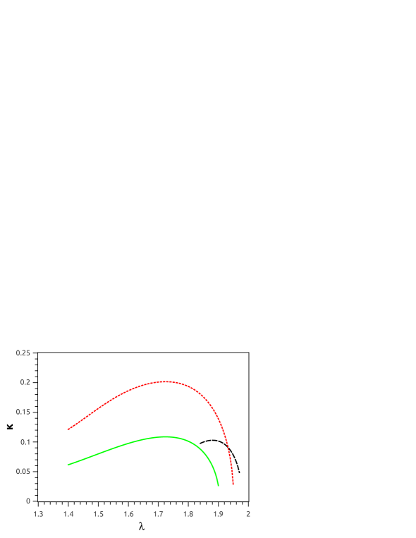
Figure 1: Variation of the acoustic surface gravity with the specific angular momentum of the flow for monotransonic polytropic accretion characterized by $\mathcal{E}=0.06,\;\;\gamma=1.333$ for three different flow geometries - namely, for flow in hydrostatic equilibrium in the vertical direction (solid green line), constant thickness flow (long dashed black line), and for the conical model (dotted red line).

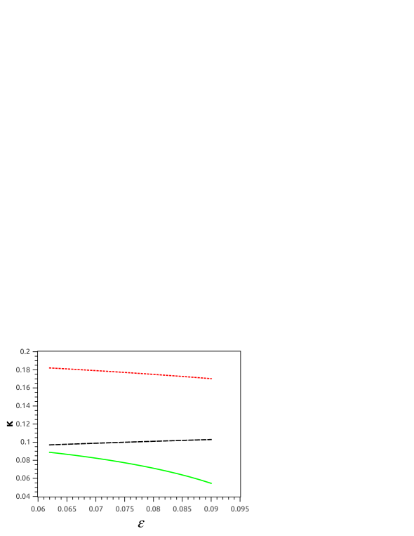
Figure 2: Variation of the acoustic surface gravity with the specific energy of the flow for monotransonic polytropic accretion characterized by $\lambda=1.835,\;\;\gamma=1.333$ for three different flow geometries - namely, for flow in hydrostatic equilibrium in the vertical direction (solid green line), constant thickness flow (long dashed black line), and for the conical model (dotted red line). Only the common range of specific energy for which all the flow configurations produce adiabatic monotransonic flow has been considered in the figure, see text for further detail.

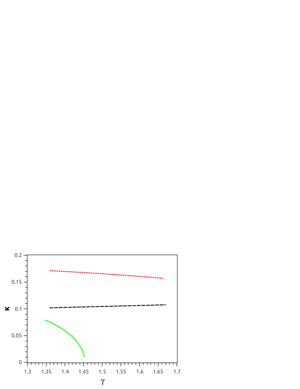
Figure 3: Variation of the acoustic surface gravity with the specific energy of the flow for monotransonic polytropic accretion characterized by $\lambda=1.85,\;\;\mathcal{E}=0.06$ for three different flow geometries - namely, for flow in hydrostatic equilibrium in the vertical direction (solid green line), constant thickness flow (long dashed black line), and for the conical model (dotted red line).

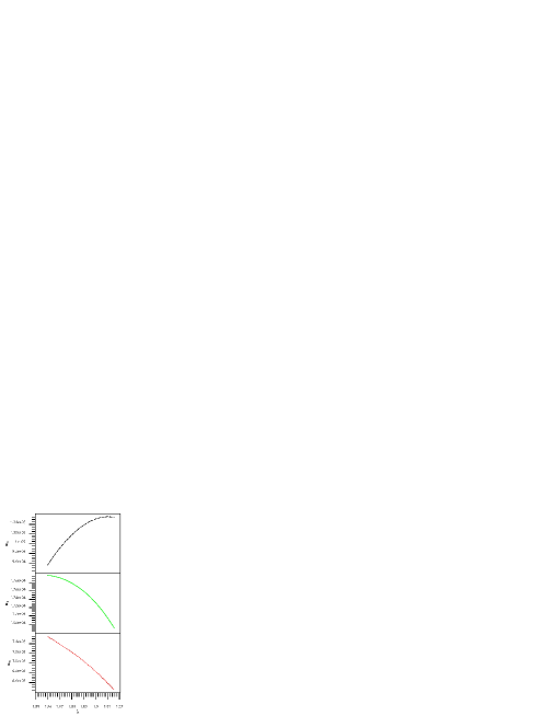
Figure 4: Variation of the ratio of the acoustic surface gravity evaluated at the inner acoustic horizon to the acoustic surface gravity evaluated at the outer acoustic horizon with the range of the specific angular momentum (for a fixed value of $\left[{\cal E}=0.0002,\gamma=4/3\right]$) of the multi-transonic flow for which a stationary shock may form.

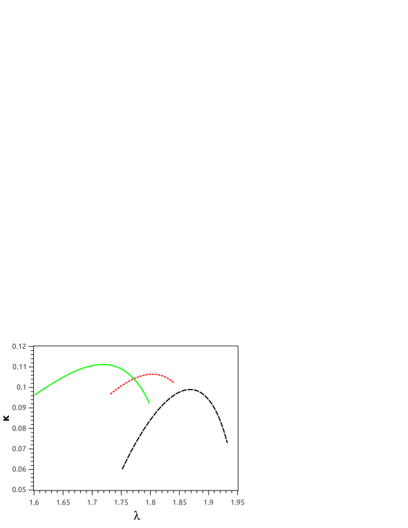
Figure 5: Variation of the acoustic surface gravity with the specific angular momentum of the flow for monotransonic isothermal accretion characterized by the isothermal flow temperature $T_{10}=22$ for three different flow geometries - namely, for flow in hydrostatic equilibrium in the vertical direction (solid green line), constant thickness flow (long dashed black line), and for the conical model (dotted red line).

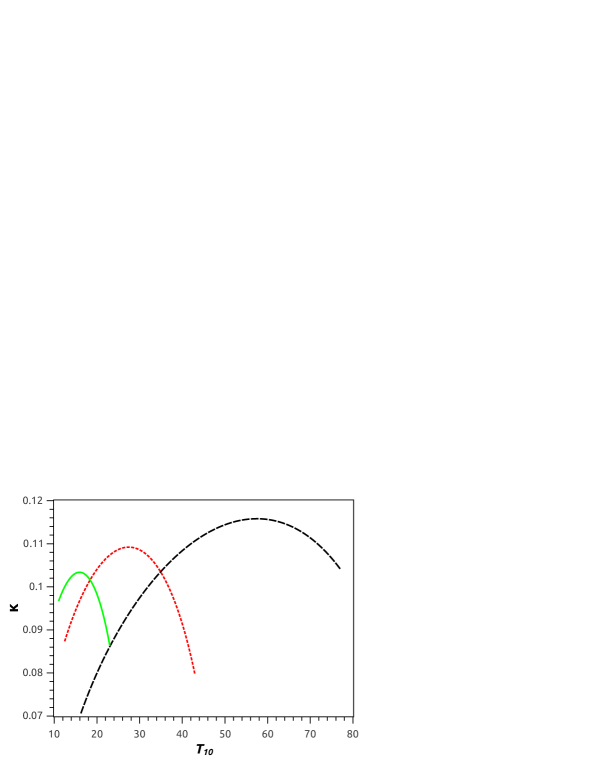
Figure 6: Variation of the acoustic surface gravity with the isothermal flow temperature of the flow for monotransonic isothermal accretion characterized by$\lambda=1.8$ for three different flow geometries - namely, for flow in hydrostatic equilibrium in the vertical direction (solid green line), constant thickness flow (long dashed black line), and for the conical model (dotted red line).

Figure 1 shows the variation of the acoustic surface gravity $\kappa$ as a function of the specific angular momentum $\lambda$ for monotransonic polytropic accretion. The specific energy ${\cal E}$ and the polytropic index $\gamma$ have been kept constant at values $\left[{\cal E}=0.06,\gamma=1.333\right]$. The range of $\lambda$ for which $\kappa$ has been calculated for a particular flow model constructs a subset in the $\left[{\cal E},\lambda,\gamma\right]$ parameter space for which the representative flow models produces mono-transonic accretion for a fixed set of values of $\left[{\cal E}\right]$. Alternative ranges for $\lambda$ for other similar subsets of $\left[{\cal E},\lambda,\gamma\right]$ parameter space may also be considered to study the ‘$\kappa-\lambda$’ profile for other fixed values of $\left[{\cal E},\gamma\right]$. The solid line (green coloured in the online version) represents the $`\kappa$ - $\lambda$’ variation profile for mono-transonic accretion in vertical equilibrium (VE), whereas the dotted (red coloured in the online version) and the long dashed (black coloured in the online version) curves represents such dependence for flow with constant height (CH) as well as for the conical flow (CM) respectively.

It is usually observed that $\kappa$ varies with $\lambda$ non linearly and non monotonically. For relatively lower values of the specific angular momentum, the acoustic surface gravity correlates with the specific angular momentum and attains a peak characterized by an unique value of the specific angular momentum denoted by $\lambda_{\rm max}$, and subsequently falls of with $\lambda$ for $\lambda>\lambda_{\rm max}$. $\lambda_{\rm max}$ is different for different flow models and one observes that

$$\lambda^{\rm CM}_{\rm max}>\lambda^{\rm VE}_{\rm max}>\lambda^{\rm CH}_{\rm max}$$ (6.1)

For a set of fixed values of $\left[{\cal E},\lambda\right]$, $\lambda_{\rm max}$ for a particular flow model can be calculated completely analytically. We illustrate such procedure for constant thickness flow. Similar procedure may be followed to calculate $\lambda_{\rm max}$ for two other flow geometries.

For constant thickness flow, eq. (5.5) provides the dependence of $\kappa$ on the critical points, the acoustic speed and its space gradient, and on the space gradient of the flow velocity itself, everything evaluated at the acoustic horizon (the critical point). $\left(c_{s}\right)_{r_{c}}$, $\left(dc_{s}/dr\right)_{r_{c}}$ and $\left(du/dr\right)_{r_{c}}$ can be expressed as a function of $r_{c}$ and $\left[{\cal E},\lambda,\gamma\right]$ using eq. (5.2) and eq. (5.1.1), respectively. The critical point $r_{c}$ itself can be computed in terms of $\left[{\cal E},\lambda,\gamma\right]$ by solving the polynomial in $r_{c}$ as represented through eq. (5.3). Hence $\kappa$ for the constant thickness flow, can be specified in terms of $\left[{\cal E},\lambda,\gamma\right]$. Analytical expression for $\kappa_{\rm CH}{\equiv}\kappa_{\rm CH}\left[{\cal E},\lambda,\gamma\right]$

can thus be maximized with respect to the specific angular momentum and the corresponding $\lambda_{\rm max}$ can thus be obtained.

From figure 1, one should note that for the common range of the specific angular momentum for which all three flow models will produce mono transonic flow for a fixed set of value of $\left[{\cal E},\lambda\right]$, does not allow to explore the complete non monotonic ‘$\kappa$ - $\lambda$’ profile for all the three flow models simultaneously. For example, for the common range of $\lambda$ as shown in the figure for which all three flow geometries produces the monotransonic accretion, $\kappa$ for constant height flow as well as for conical model accretion will anti correlates with $\lambda$, whereas for full range of allowed $\lambda$ to form mono transonic accretion at individual level, ‘$\kappa$ - $\lambda$’ profile for both the aforementioned flows exhibits a maximum.

Similar features are observed for the ‘$\kappa$ - ${\cal E}$’ profile, which has been shown in the figure 2, where the $\kappa$ vs ${\cal E}$ variation (for a fixed set of $\left[\lambda,\gamma\right]$) for constant height flow apparently shows that $\kappa_{\rm CH}$ correlates with ${\cal E}$, whereas $\kappa_{\rm CM}$ and $\kappa_{\rm VE}$ anti-correlates with ${\cal E}$. Such trend, however, does not provide the complete information about the ‘$\kappa$ - ${\cal E}$’ profile in general since the range of ${\cal E}$ for which the figure is drawn is actually taken from the common region of $\left[{\cal E},\lambda,\gamma\right]$ space for which all three flow geometries produces mono transonic accretion for a fixed value of $\left[\lambda,\gamma\right]$. If one allows $\kappa$ to vary with ${\cal E}$ for the entire range of the specific energy for which a particular flow model provides the mono transonic accretion for a fixed value of $\left[\lambda,\gamma\right]$, $\kappa$ vs ${\cal E}$ profile would have a non monotonic behaviour with a corresponding ${\cal E}_{\rm max}$ separately for every flow configuration. The corresponding ${\cal E}_{\rm max}$ for every flow model could then be estimated by maximizing the expression for the acoustic surface gravity with respect to ${\cal E}$ by keeping $\left[\lambda,\gamma\right]$ constant. One thus understands that the ‘anti correlating’ $\kappa$ vs ${\cal E}$ profile for the conical flow (represented by the dotted red curve) as well as for flow in the hydrostatic equilibrium along the vertical direction (solid green curve), respectively, are thus the post-peak (${\cal E}>{\cal E}_{\rm max}$) descending part of the complete non monotonic ‘$\kappa$ - ${\cal E}$’ profiles for the corresponding flow configuration. Similarly, the ‘correlating’ $\kappa$ - ${\cal E}$ profile for the constant height flow (represented by the long dashed black curve) is actually the pre-peak (${\cal E}<{\cal E}_{\rm max}$) ascending part of the complete non monotonic $\kappa$ - ${\cal E}$ profile for the corresponding flow geometry. Hence ${\cal E}^{\rm CH}_{\rm max}$ is largest among all the values of ${\cal E}_{\rm max}$ corresponding to all three different flow configurations.

Figure 3 shows the $\kappa$ - $\gamma$ profile (for a fixed set of $\left[{\cal E},\lambda\right]$). It is obvious from the figure that ${\gamma}^{\rm CH}_{\rm max}$ has the largest value among all three values of ${\gamma}_{\rm max}$ corresponding to three different flow configurations. ${\cal E}_{\rm max}$ and $\gamma_{\rm max}$ for any particular model can also be estimated by maximizing $\kappa$ with respect to the respective parameters.

One thus understands that for monotransonic adiabatic accretion characterized by a fixed set of values of $\left[{\cal E},\lambda,\gamma\right]$, the analogue surface gravity for three different flow configurations exhibit the following trend

$$\kappa_{\text{\tiny CM}}^{\rm adia}~{}>~{}\kappa_{\text{\tiny VE}}^{\rm adia}~{}>~{}\kappa_{\text{\tiny CH}}^{\rm adia}$$ (6.2)

Hence for the adiabatic mono transonic accretion, flow in conical shape produces the largest value of the analogue Hawking like temperature whereas the flow with constant thickness provides the lowest value of $T_{AH}$ for the same set of initial boundary conditions.

As has been mentioned in section 4.1, multi-transonic accretion with stationary shock may be realized for all three different flow configurations for adiabatic as well as for isothermal accretion, studied here in this work. For such flow topologies, two black hole type acoustic horizons form at the inner and the outer saddle type sonic points. The corresponding acoustic surface gravity $\kappa_{in}$ and $\kappa_{out}$ can be evaluated at the inner and the outer sonic points respectively. We define

$$\kappa_{io}=\frac{\kappa_{in}}{\kappa_{out}}$$ (6.3)

It has been observed that the overall $\left(\kappa_{in}-\left[{\cal E},\lambda,\gamma\right]\right)$ as well as the $\left(\kappa_{out}-\left[{\cal E},\lambda,\gamma\right]\right)$ profiles are qualitatively similar with the $\left(\kappa-\left[{\cal E},\lambda,\gamma\right]\right)$ profile for all three flow configurations, where $\kappa$ is the acoustic surface gravity evaluated for the mono transonic accretion. For all three flow geometries considered in this work, the value of $\kappa_{out}$ is, however, several orders of magnitude less than that of the corresponding $\kappa_{in}$ for same set of initial boundary conditions. This is because the outer acoustic horizons form at a large distance away from the black hole event horizon compared to the location of the inner acoustic horizon with respect to the black hole event horizon. For a typical set of the initial boundary conditions, the inner acoustic horizon may form 1.5 - 5 Schwarzschild radius away from the black hole event horizon whereas the outer acoustic horizon may be located at $10^{3}$ - $10^{6}$ Schwarzschild radius away, or even more, from the black hole event horizon. Weak gravity at such a large distance (where the outer sonic horizons form) restrict the acoustic surface gravity to possess such a small numerical value. Same argument applies for the analogue Hawking temperatures evaluated at the inner and the outer acoustic horizons as well.

In figure 4, we plot $\kappa_{io}$ as a function of $\lambda$ for the constant thickness flow (uppermost panel), flow in hydrostatic equilibrium along the vertical direction (mid panel) and for the conical flow (lowermost panel). The range of $\lambda$ used in this figure corresponds to the common value of the specific angular momentum for which shock forms for multi-transonic accretion in all three flow geometries for a fixed value of $\left[{\cal E},\lambda\right]$. The common range of $\lambda$ is chosen in such a way so that the inner acoustic horizon forms at a distance larger than two Schwarzschild radius from the black hole event horizon. Since we use pseudo Schwarzschild potentials which are relatively less reliable in simulating the general relativistic space time extremely close to the black hole event horizon, we prefer to confine our attention to the mono transonic as well as the multi transonic flow topologies for which the acoustic horizon does not form at a very close proximity to the black hole event horizon. From the figure it is evident that

$$\lambda^{\rm CM}_{\rm max}>\lambda^{\rm VE}_{\rm max}>\lambda^{\rm CH}_{\rm max}$$ (6.4)

where $\lambda_{\rm max}$ in eq. (6.4) is the value of $\lambda$ for which the non monotonic $\kappa_{io}$ - $\lambda$ profile attains its maximum. Interestingly enough, eq. (6.1) is identical with eq. (6.4), indicating the fact that the dependence of the acoustic surface gravity on initial boundary conditions is similar for both the mono as well as for the multi-transonic shocked accretion in all three flow geometries considered here in this work. Once again, the $\kappa_{io}$ - $\lambda$ dependence does not exhibit the peaked non monotonic profile since the common range corresponding to the shock forming $\lambda$ is not sufficient to provide the required span for the $\kappa_{io}$ - $\lambda$ variation for any particular flow geometry for the entire range of $\lambda$ for which the corresponding flow model produces shocked multi-transonic accretion for a fixed value of $\left[{\cal E},\lambda\right]$.

Figure 5 demonstrates the dependence of the acoustic surface gravity on specific angular momentum for mono transonic isothermal accretion for three different flow models. It is observed that

$$\lambda^{\rm CM}_{\rm max}>\lambda^{\rm VE}_{\rm max}>\lambda^{\rm CH}_{\rm max}$$ (6.5)

In figure 6, we plot the dependence of $\kappa$ on the isothermal flow temperature $T$ (scaled by a factor of $10^{10}$ degree Kelvin - $T_{10}{\equiv}T{\times}{10^{-10}}$). We obtain

$$T^{\rm CM}_{\rm max}>T^{\rm VE}_{\rm max}>T^{\rm CH}_{\rm max}$$ (6.6)

The value of $\lambda_{\rm max}$ and $T_{\rm max}$ for the monotransonic isothermal flow may be estimated for all three flow geometries in a way similar to what has been accomplished for the polytropic flow.

7 Discussion

Axisymmetric accretion onto a non-rotating astrophysical black hole under the influence of pseudo-Schwarzschild potentials are natural example of classical analogue systems found in the universe. The corresponding acoustic geometry may be studied for three different flow configurations, viz, accretion with constant flow thickness, the conical flow, and accretion disc in hydrostatic equilibrium in the vertical direction. For each background flow geometry, all together eight different configurations for the acoustic geometry - adiabatic as well as isothermal accretion for four different pseudo-potentials, may be studied. For any specific pseudo potential, six different configurations of the acoustic flow geometry - adiabatic as well as isothermal accretion in three different flow geometries, may be studied. For any geometric configuration of the adiabatic flow under the influence of a particular potential, the three initial parameters, viz., the specific energy ${\cal E}$, the specific angular momentum $\lambda$, and the adiabatic index of the flow $\gamma$ can completely specify the corresponding acoustic geometry. Similarly for the isothermal flow in any potential and with any flow geometry, the two initial parameters, viz., the constant flow temperature $T$ and the specific angular momentum $\lambda$, can completely specify the corresponding acoustic geometry.

Among six possible flow configurations for any particular pseudo potential used, only the adiabatic flow in vertical equilibrium exhibits an ‘effective’ sound speed which is a scaled version of the adiabatic sound speed with a $\gamma$ dependent scaling constant. The scaling constant becomes unity for isothermal flow. The reason is that for the accretion in vertical equilibrium the flow thickness is a function of the adiabatic sound speed, as well as a function of the space derivative of the pseudo-potential used, since the expression for such flow thickness is obtained by balancing the pressure gradient with the relevant component of the gravitational force. One should, however, bear in mind that the corresponding expressions for the flow thickness in all three flow geometries used are derived using a set of idealized assumptions. In principle, a more realistic derivation of the flow thickness may be worked out by employing the non-LTE radiative transfer (see [39, 40] ) or by taking recourse to the Grad-Shafranov equations for MHD flow (see [41, 42, 43] ).

For multi-transonic flow, two acoustic black holes are formed at two regular saddle type sonic points, whereas the acoustic white hope forms at the shock location, in agreement with the results obtained by [19] and [8] . The acoustic surface gravity is formally infinite for the acoustic white hole since the flow velocity as well as the sound speed changes discontinuously at the shock location, in agreement with the findings of [44] .

The surface gravity $\kappa$ (or $T_{\rm AH}$) profile obtained for the multi-transonic flow at the inner acoustic horizon is similar to the $\kappa$ profile for mono-transonic flow. This indicates that irrespective of the phase topology, the surface gravity is basically determined by the physical proximity of the acoustic horizon to the black hole event horizon. This is further supported by the fact that irrespective of the flow geometry, pseudo potentials or the equation of state used to describe the accretion flow, the value of $\kappa$ at the outer acoustic horizon (for multi-transonic flow) is much less than that evaluated at the inner acoustic horizon.

For a fixed set of $\left[{\cal E},\lambda,\gamma\right]$ describing the adiabatic accretion as well as for a fixed set of $\left[T,\lambda\right]$ describing the isothermal accretion, the conical flow produces the largest whereas the flow with constant thickness the smallest surface gravity and the analogue Hawking temperature. The accretion flow in the hydrostatic equilibrium in the vertical direction provides the value of $\kappa$ and $T_{\rm AH}$ in between the respective values of $\kappa$ and $T_{\rm AH}$ for the conical and the constant thickness flow, respectively. The influence of the flow geometry in determining the acoustic surface gravity has thus been successfully investigated in this work.

One of our major achievements is the computation of the acoustic surface gravity and the investigation of its dependence on various flow geometries and on various accretion parameters completely analytically.. However, one should note that this has been possible owing to a specific feature of the chosen pseudo potential. With the Paczyński & Wiita (1980) potential $\Phi_{1}=-\frac{1}{2\left(r-1\right)}$, the energy first integral for the adiabatic accretion (see eq. (4.12) as well as the critical point condition for the isothermal flow (see eq. (5.1.1 - 5.1.2)) can be recast into a fourth degree polynomial in ${r_{c}}$ (equivalently, in ${r_{h}}$) in an exactly solvable form. This has not been possible with other pseudo potentials, for which such an exactly solvable polynomial in ${r_{h}}$ can not be constructed. With other potentials, however, the surface gravity $\kappa$ can still be studied as a function of various flow parameters and flow geometries, with the help of numerical methods. Remarkably, it has been demonstrated in the literature ([16, 17] and references therein) that out of the four pseudo Schwarzsculd potentials as shown in eq. (5.1.2), the potential $\Phi_{1}$ mimics the Schwarzschild space time most efficiently in constructing the integral flow solution for transonic accretion.

However, even if one can not employ a complete analytical calculation and even if $\Phi_{1}$ is the most suitable potential to mimic a Schwarzschild space time, our generalized formalism for the evaluation of $\left[u,c_{s},dc_{s}/dr,du/dr\right]_{r_{h}}$ and the corresponding values of $\kappa$ and $T_{\rm AH}$ in terms of a general $\Phi$ is still important in the following sense. There exists a possibility that a new form of $\Phi$ more effective than $\Phi_{1}$ will be suggested in the future in order to approximate the Schwarzschild space time in constructing the integral accretion solutions for the transonic flow. In such a case, if a general model is capable of computing the acoustic surface gravity (and hence the analogue Hawking temperature) in a way presented in this work, then this model will be able to readily accommodate that novel form of the pseudo-Schwarzschild potential with no need to significantly change the fundamental structure of the formulation and the solution scheme. In this case one need not worry about providing any new unique scheme valid exclusively only for a particular form of pseudo potential.

The methodology developed in this paper can also be used to construct the relevant acoustic geometry for the equatorial slice of the accretion flow under the influence of various pseudo-Kerr potentials as well to study the variation of the surface gravity with the black hole spin. Such work is in progress and will be reported elsewhere.

However, one should be cautious when using the pseudo potentials because none of the potentials discussed here can be directly derived from the Einstein equations. These potentials are used to obtain more accurate correction terms over and above the pure Newtonian results. Hence any ‘radically new’ results obtained using these potentials should be cross checked very carefully against general relativity. Besides, one should bear in mind that these potentials are not too reliable for modeling the space time in the very close neighborhood of the event horizon since strong gravity effects dominate in this region. Hence our formalism may not be quite realistic if the acoustic horizon forms very close to the black hole event horizon. We thus consider only those initial boundary conditions for which ${r_{h}>2}$ ensuring our findings to be trustworthy.

References

- [1] Novello, Visser, and Volovik, eds., Artificial Black Holes. World Scientific, Singapore, 2002.
- [2] V. Cardoso, “Acoustic black holes.” physics/0503042, 2005.
- [3] C. Berceló, S. Liberati, and M. Visser, Analogue gravity, Living Reviews in Relativity 8 (2005), no. 12.
- [4] R. Schtzhold and W. H. Unruh, eds., Quantum Analogues: From Phase Transitions to Black Holes and Cosmology. Springer, Berlin, 2007.
- [5] T. K. Das Class. Quant. Grav. 21 (2004) 5253.
- [6] S. Kinoshita, Y. Sendouda, and K. Takahashi Phys. Rev. D 70 (2004) 123006.
- [7] S. Dasgupta, N. Bili, and T. K. Das General Relativity & Gravitation (GRG) 37 (2005), no. 11 1877 – 1890.
- [8] H. Abraham, N. Bilić, and T. K. Das Classical and Quantum Gravity 23 (2006) 2371.
- [9] T. Naskar, N. Chakravarty, J. K. Bhattacharjee, and A. K. Ray Physical Review D 76 (2007), no. 12 123002.
- [10] T. K. Das, N. Bilić, and S. Dasgupta JCAP 2007 (2007), no. 06.
- [11] P. Mach and E. Malec Physical Review D 78 (2008), no. Issue 12 124016.
- [12] P. Mach Reports on Mathematical Physics 64 (2009), no. issue 1-2 257 – 269.
- [13] Pu, Maity, Das, and Chang, “On spin dependence of relativistic acoustic geometry.”.
- [14] M. A. Abramowicz and W. H. Zurek.
- [15] S. Kato, J. Fukue, and S. Mineshige, Black Hole Accretion Disc. Kyoto University Press, 1998.
- [16] I. V. Artemova, G. Björnsson, and I. D. Novikov ApJ 461 (1996) 565.
- [17] T. K. Das ApJ 577 (2002) 880.
- [18] S. Nag, S. Acharya, A. K. Ray, and T. K. Das New Astronomy 17 (2012) 285 – 295.
- [19] C. Berceló, S. Liberati, S. Sonego, and M. Visser New Journal of Physics 6 (2004), no. 1 186.
- [20] W. G. Unruh Phys. Rev. Lett. 46 (1981) 1351.
- [21] T. A. Jacobson Phys. Rev. D. 51 (1991) 2827.
- [22] W. G. Unruh Phys. Rev. D 51 (1995) 2827.
- [23] M. Visser Class. Quant. Grav. 15 (1998) 1767.
- [24] T. A. Jacobson Prog. Theor. Phys. Suppl. 136 (1999) 1.
- [25] V. Moncrief ApJ. 235 (1980) 1038.
- [26] N. Bili Class. Quant. Grav. 16 (1999) 3953.
- [27] T. K. Das, J. K. Pendharkar, and S. Mitra ApJ 592 (2003) 1078.
- [28] T. K. Das and B. Czerny New Astronomy 17 (2012), no. 3 254–271.
- [29] A. M. Beloborodov and A. F. Illarionov MNRAS 323 (1991) 167.
- [30] I. V. Igumenshchev and A. M. Beloborodov MNRAS 284 (1997) 767.
- [31] D. Proga and M. C. Begelman ApJ. 582 (2003) 69.
- [32] B. Paczyński and P. J. Wiita A & A 88 (1980) 23.
- [33] M. A. Nowak and R. V. Wagoner ApJ. 378 (1991) 656.
- [34] R. Matsumoto, S. Kato, J. Fukue, and A. T. Okazaki PASJ 36 (1984) 71.
- [35] J. Frank, A. King, and D. Raine, Accretion Power in Astrophysics. Cambridge University Press, Cambridge, 2002.
- [36] O. Blaes MNRAS 227 (1987) 975.
- [37] S. Chakrabarti and S. Das MNRAS 327 (2001) 808.
- [38] A. G. Kurosh, Higher Algebra. Mir Publication, Moscow, 1972.
- [39] I. Hubeny and V. Hubeny ApJ 505 (1998) 558.
- [40] S. W. Davis and I. Hubeny ApJS 164 (2006) 530.
- [41] V. S. Beskin Phys. -Usp. 40 (1997) 659.
- [42] V. S. Beskin and A. Tchekhovskoy A & A 433 (2005) 619.
- [43] V. S. Beskin, MHD Flows in Compact Astrophysical Objects: Accretion, Winds and Jets. Springer, 2009.
- [44] S. Liberati, S. Sonego, and M. Visser Classical and Quantum Gravity 17 (2000), no. 15 2903 – 2923.