Disorder-induced cavities, resonances, and lasing in randomly-layered media

Abstract

We study, theoretically and experimentally, disorder-induced resonances in randomly-layered samples,and develop an algorithm for the detection and characterization of the effective cavities that give rise to these resonances. This algorithm enables us to find the eigen-frequencies and pinpoint the locations of the resonant cavities that appear in individual realizations of random samples, for arbitrary distributions of the widths and refractive indices of the layers. Each cavity is formed in a region whose size is a few localization lengths. Its eigen-frequency is independent of the location inside the sample, and does not change if the total length of the sample is increased by, for example, adding more scatterers on the sides. We show that the total number of cavities, $N_{\mathrm{cav}}$, and resonances, $N_{\mathrm{res}}$, per unit frequency interval is uniquely determined by the size of the disordered system and is independent of the strength of the disorder. In an active, amplifying medium, part of the cavities may host lasing modes whose number is less than $N_{\mathrm{res}}$. The ensemble of lasing cavities behaves as distributed feedback lasers, provided that the gain of the medium exceeds the lasing threshold, which is specific for each cavity. We present the results of experiments carried out with single-mode optical fibers with gain and randomly-located resonant Bragg reflectors (periodic gratings). When the fiber was illuminated by a pumping laser with an intensity high enough to overcome the lasing threshold, the resonances revealed themselves by peaks in the emission spectrum. Our experimental results are in a good agreement with the theory presented here.

I Introduction

Anderson localization of waves in one-dimensional random media is associated with an exponential decrease of the wave amplitude inside the disordered, locally-transparent sample, which results in an exponentially small typical transmittance $T_{\mathrm{typ}}\varpropto\exp\left(-L/l_{\mathrm{loc}}\right)\ll 1$ (where $L$ is the length of the sample, and $l_{\mathrm{loc}}$ is the localization length). Another manifestation of Anderson localization is the existence of resonant frequencies, where the transmission increases drastically, sometimes up to unity. These frequencies correspond to the quasi-localized eigenstates (modes, or disorder-induced resonances) characterized by a high concentration of energy in randomly-located points inside the system.

Even though one-dimensional (1D) localization has been intensively studied during the last few decades 50 years (see also LGP ; Ping and references therein), most of the analytical results were obtained for mean quantities, i.e., for values averaged over ensembles of random realizations. These results are physically meaningful for the self-averaging Lyapunov exponent (inverse localization length), which becomes non-random in the macroscopic limit LGP . For non-self-averaging quantities (field amplitude and phase, intensity, transmission and refection coefficients, etc.) a random system of any size is always mesoscopic, and therefore, mean values have little to do with measurements at individual samples. This is most pronounced when it comes to the disorder-induced resonances whose parameters are extremely volatile and strongly fluctuate from realization to realization Azbel1 ; Azbel2 . In particular, ensemble averaging wipes out all information about the frequencies and locations of individual localized states within a particular sample, even though these data are essential for applications based on harnessing micro and nano cavities with high $Q$-factors.

I.1 Disorder-induced cavities and resonances

Nowadays, photonic crystals are believed to be the most suitable platforms for the creation and integration of optical resonators into optical networks. To create an effective resonant cavity that supports localized high-$Q$ modes in a photonic crystal (PC), it is necessary to break periodicity, i.e. to introduce a defect in a regular system. As fluctuations of the dielectric and geometrical parameters are inevitably present in any manufactured periodic sample, it could create a serious obstacle in the efficient practical use of PCs. Therefore considerable efforts of researches and manufacturers go into the control of fluctuations. Alternatively, if rather than combating imperfections of periodicity, one fabricated highly-disordered samples, they could be equally well harnessed, for example, for creating tunable resonant elements. This is because 1D random configurations have a unique band structure that for some applications have obvious advantages over those of PC Genack we 1 . Contrary to periodic systems, resonant cavities inherently exist in any (long enough) disordered sample, or can be easily created by introducing a non-random element (for example, homogeneous segment) into an otherwise random configuration. The effective wave parameters of these cavities are very sensitive to the fine structure of each sample, and can be easily tuned either by slightly varying the refractive index in a small area inside the sample or, for example, by changing the ratio between the coupling strength and absorption. This makes possible to shift the resonant frequency (and thereby to lock and unlock the flow of radiation); to couple modes and create quasi-extended states, etc Genack we 2 ; Labonte .

It has been shown JOSA that each localized state at a frequency $\omega=\omega_{\mathrm{res}}$ could be associated with an effective, high $Q$-factor resonance cavity comprised of almost transparent (for this frequency) segment bounded by essentially non-transparent regions (effective barriers). Wave tunneling through such a system can be treated as a particular case of the general problem of the transmission through an open resonator Colloquium . The distinguishing feature of a disorder-induced cavity is that it has no regular walls (the medium is locally transparent in each point), and high reflectivity of the confining barriers is due to the Anderson localization. Moreover, different segments of the sample are transparent for different frequencies, i.e., each localized mode is associated with its own resonator.

I.2 Random lasers

If the medium inside such a cavity is amplifying, the combination of the optical gain and the interference of multiply scattered radiation creates coherent field and gives rise to multi-frequency lasing with sharply peaked lasing spectrum. Random lasers (RL) are the subject of increasing scientific interest due to their unusual properties and promising potential applications Cao1 ; Noginov ; Cao99 ; Ara ; Patrick new 1 ; Patrick new 2 ; RLasers . Unlike conventional lasers, where any disorder is detrimental, in a random version, scattering plays a positive role increasing the path length and the dwell time of light in the active medium. So far most studies, both experimental and theoretical, have concentrated on 3D disordered systems and chaotic cavities. One of the grave drawbacks of 3D random lasers is their inefficient pumping, which is hampered by the scattering of the pumping radiation in the random medium. A one-dimensional RL, which is free from this disadvantage, can be realized either as a random stack of amplifying layers Genack2004 or as a set of Bragg gratings randomly distributed along a doped optical fiber Noemi . In the last case, the wavelength of the pumping laser is shifted from the Bragg resonance of the gratings, and the fiber is excited homogeneously along the whole length of the sample. Both these methods reduce noticeably the lasing threshold as compared to 3D random lasing systems. Because the frequencies of the modes and the locations of the effective cavities vary from sample to sample randomly, in the most cases they are described statistically Misirpashaev98 ; Zaitsev06 ; Zaitzev09 ; Soukoulis2000 ; Cao2007 . However, usually we deal with a specific random sample, and it is important to know how many modes and at which frequencies can be excited in a given frequency range; where these modes are localized inside this sample, etc Patrick new 1 .

Another field of research in which this information is crucial has arisen recently after it had been realized that Anderson resonances could be used to observe cavity quantum electrodynamics effects by embedding a single quantized emitter (quantum dot) in a disordered PC waveguide Lodahl-1 ; Lodahl-2 . In those experiments, the efficiency of the interaction between radiation and disorder-induced cavities depends strongly on the location of the source inside the random sample. Indeed, all QED effects are well-pronounced when the emitter with a given frequency is placed inside the effective cavity, which is resonant at this frequency, and could be completely suppressed otherwise.

In this paper, we develop an algorithm that enables to detect all cavities and to find their locations and eigen-frequencies for any individual sample with given geometry and optical parameters. It is shown that in the case of uncorrelated disorder, the number of disorder-induced resonances per unit frequency interval is independent of the strength of the fluctuations and is uniquely determined by the size of the random sample. The results have been checked experimentally using RLs based on a single-mode fiber with randomly distributed resonant Bragg gratings developed in Noemi .

II Disorder-induced cavities and resonances

It has been shown in JOSA ; Colloquium ; Genack we 1 ; Genack we 2 that for a quantitative description of the wave propagation through a disordered sample, it is advantageous to consider it as a random chain of effective regular resonators with given Q-factors and coupling coefficients. The typical size of each resonator is of the order of the localization length, $l_{\mathrm{loc}}$, and their centers are randomly distributed along the sample. For manufacturing RLs and for the ability to tailor their properties, it is important to know the location of the resonant cavity for each eigen-frequency Patrick new 1 . To this end, a criterion is necessary, which enables to determine whether a given area of a disordered sample is either a resonant cavity or a strongly reflecting (typical) random segment.

To derive such a criterion for randomly layered media, we consider a disordered sample consisting of $N$  homogeneous layers with thicknesses $d_{j}$ and dispersionless refractive indices $n_{j}$ ($j=1,2,\ldots,N$) that are statistically independent and uniformly distributed in the intervals $(d_{0}-\delta\!d,d_{0}+\delta\!d)$ and ($n_{0}-\delta\!n,n_{0}+\delta\!n)$, respectively. (The effects of correlation between the thicknesses of the adjacent blocks have been considered in FN 1 ; FN 2 ; FN 3 ). In a system with uncorrelated layers, the interface between the $j$-th and $(j+1)$-th layers is located at a random point $z_{j}$ and can be characterized by complex transmission, $t_{j}$, and reflection, $r_{j}$, coefficients, which are also randomly distributed in the corresponding intervals. The numeration is chosen from left to right so that $z_{j}<z_{j+1}$. It is assumed thereafter that the optical contrast between layers is small. Therefore all Fresnel reflection coefficients $r_{j}$ are also small

$$|r_{j}|\ll 1$$ (1)

and, consequently, $1-|t_{j}|^{2}\ll 1$. For the sake of simplicity these coefficients will be assumed real. Generalization to complex-valued $r_{j}$ and $t_{j}$ is straightforward.

In what follows, it is convenient to turn to the optical lengths, i.e. to replace the thicknesses $d_{j}$ and the coordinates $z_{j}$ by

$$\tilde{d}_{j} = n_{j}d_{j},$$

$$\tilde{z}_{j} = \sum_{i<j}n_{i}z_{i},$$ (2)

where $n_{j}$ is the refraction index of the $j$-th layer. Note that in these notations the wave number has the same value $\widetilde{k}=k=\omega/c$ in all layers.

To distinguish between an effective resonator and a Bragg reflector, a proper physical quantity representative of distinctive properties of these objects has to be found. To do this, let us consider a wave that propagates rightward from a point $\tilde{z}=\tilde{z}_{j}+0$ [right side of the interface between the $(j-1)$-th and $j$-th layers], where its amplitude is $A_{j0}^{(+)}$ (thereafter superscripts $(+)$ and $(-)$ denote the amplitudes of the waves propagating to the right or to the left, respectively). After traveling through the $j$-th layer, the wave is partially reflected back from the interface between the $j$-th and $(j+1)$-th slabs. The transmitted part extends through $(j+1)$-th layer and is partially reflected from the next interface, etc. (see Fig. 1).

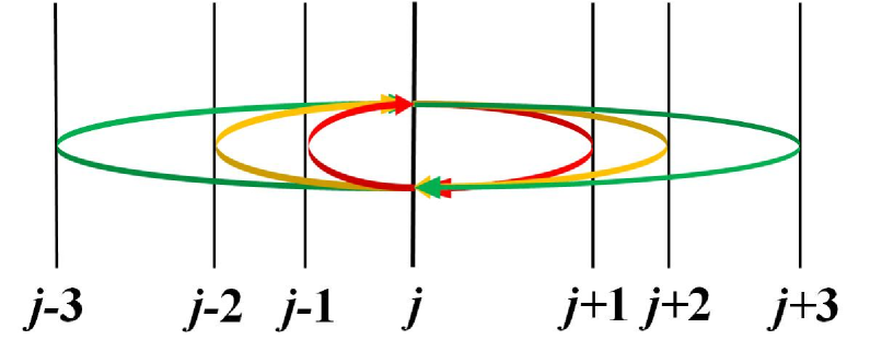
Figure 1: (color online) Schematic diagram of closed trajectories in a randomly-layered sample.

If the scattering at the interfaces between layers is weak, Eq. (1), the amplitude $\tilde{A}_{j}^{(-)}$ of the total field reflected from $N_{s}$ layers and returned back to the point $\tilde{z}=\tilde{z}_{j}+0$ can be calculated in the single-scattering approximation, and is equal to:

$$\tilde{A}_{j}^{(-)}=r_{j}^{(+)}(k)\,A_{j0}^{(+)},$$ (3)

where

$$r_{j}^{(+)}(k)=\sum_{m=1}^{N_{s}}r_{j+m}\,\exp\left[2ik\left(\tilde{z}_{j+m}-\tilde{z}_{j}\right)\right],$$ (4)

and $k=\omega/c$ is the wave number. The amplitude $\tilde{A}_{j}^{(+)}=r_{j}^{(-)}(k)\,A_{j0}^{(-)}$ is introduced in the same way, with the left reflection coefficient $r_{j}^{(-)}(k)$

$$r_{j}^{(-)}(k)=-\sum_{m=0}^{N_{s}}r_{j-m}\;\exp\left[2ik\left(\tilde{z}_{j}-\tilde{z}_{j-m}\right)\right].$$ (5)

It is taken into account in Eq. (5) that the reflection coefficients $r_{l}$ and $r_{r}$ for waves that are incident on the same interface from the left or from the right have opposite signs: $r_{l}=-r_{r}$. The field of all waves that made a closed path and returned back after consequent reflections from $N_{s}$ layers located on the right, and $N_{s}$ layers located on the left from the $j$-th layer, has an amplitude $A_{j1}^{(+)}$. In the general case, $A_{j1}^{(+)}$ is not equal to the initial amplitude $A_{j0}^{(+)}$, and the difference is

$$\delta A_{j}^{(+)}=A_{j0}^{(+)}-A_{j1}^{(+)}\equiv A_{j0}^{(+)}\left[1-\Delta_{j}(k)\right],$$ (6)

where

$$\Delta_{j}(k)=r_{j}^{(+)}(k)\;r_{j}^{(-)}(k).$$ (7)

The function $\Delta_{j}(k)$ is an important characteristic, which uniquely determines the resonant properties of any one-dimensional wave system. In particular, the eigen-numbers can be found as poles of the Green function, i.e. as the roots of the equation brekhovsk ; Burin2002

$$\Delta_{j}(k)-1\equiv r_{j}^{(+)}(k)\,r_{j}^{(-)}(k)-1=0.$$ (8)

In the case of a closed resonator

$$\Delta(k)=\exp\left(2i\pi n\right),\hskip 8.53581ptn=1,2,3\ldots,$$

i.e. $\arg\,\Delta(k)=2\pi n$, and $\mathrm{Re}\,\Delta(k)=1$. For an open resonant cavity, the roots $k_{\mathrm{res}}$ of Eq. (8) are complex, $k_{\mathrm{res}}=k_{R}+ik_{I}$. If the Q-factor of a resonator is large enough, then $k_{R}\gg k_{I}$ and

$$\mathrm{Re}\,\Delta(k_{R}) = 1-k_{R}\ell/Q\ >0,$$ (9)

$$\mathrm{Im}\,\Delta(k_{R}) \simeq 0,$$ (10)

where $\ell$ is the resonator length.

Note that equation (10) is fulfilled also when $\arg\Delta(k)=\pi n$, which is the Bragg reflection condition. In this case, in contrast to a resonant cavity, $\mathrm{sgn}\{r^{(+)}(k)\}=-\mathrm{sgn}\{r^{(-)}(k)\}$ and the real part of $\Delta(k)$ is negative, $\mathrm{Re}\,\Delta(k)<0$.

These properties of the quantity $\Delta(k)$ are quite general and can be used to characterize randomly layered systems, in particular, to detect effective resonant cavities inside them. Indeed, when for a segment of $2N_{s}$ layers centered at a point $\tilde{z}_{j}$ inside a long ($N\gg N_{s}$) disordered sample the imaginary part of $\Delta(k)$ is zero at some $k=\omega/c$, this area is either a resonant (at the frequency $\omega$) cavity or a localization-induced resonant Bragg reflector. What it is indeed is determined by the sign of the real part of $\Delta$: in a resonator $\mathrm{Re}\,\Delta>0$, while for a Bragg grating $\mathrm{Re}\,\Delta<0.$

The last condition is easy to understand if we notice that $r_{j}^{(+)}(k)$ is $(-2k)$-Fourier harmonics of the function

$$F_{j}^{(+)}(z)=\sum_{m=1}^{N_{s}}r_{j+m}\,\delta[\tilde{z}-(\tilde{z}_{j+m}-\tilde{z}_{j})],$$ (11)

and $r_{j}^{(-)}(k)$ is the $(+2k)$-Fourier harmonics of the function

$$F_{j}^{(-)}(z)=\sum_{m=0}^{N_{s}}(-r_{j-m})\,\delta[\tilde{z}-(\tilde{z}_{j-m}-\tilde{z}_{j})].$$ (12)

This means that $r_{j}^{(+)}(k)$ and $r_{j}^{(-)}(k)$ are Bragg reflection coefficients from $N_{s}$ slabs located to the right and to the left from the $j$-th layer, respectively.

Since our prime interest here are disorder-induced resonators for which $\left|r_{j}^{(\pm)}\right|\sim 1$, and because in the localized regime the reflection coefficient from a typical region is close to unity when its length is of the order (and larger) of the localization length, for further calculations we have to choose $N_{s}=l_{\mathrm{loc}}/d_{0}\equiv N_{\mathrm{loc}}$. Important to stress that each resonator is formed in an area of the size of a few localization lengths and is practically unaffected by the outer (to this area) parts of the sample. This means that the eigen-frequency of an effective cavity is independent of it location inside a sample, and does not change if the total length of the sample is increased, for example, by adding more scatterers at its edges. When the thicknesses of the layers are uncorrelated and the mean thickness $\overline{\tilde{d_{j}}}=\widetilde{d}_{0}$ is large compared to the wavelength, $k\widetilde{d_{0}}\gg 2\pi$, the localization length is determined by the mean value of the local reflection coefficients $r_{j}$ Lianskii . To prove this statement, note that the functions $r_{j}^{(\pm)}(k)$, Eqs. (4,5), are sums of $N_{\mathrm{loc}}$ uncorrelated random complex numbers, and therefore can be described in terms of a random walk on the plane $(\mathrm{Re}\,r,\,\mathrm{Im}\,r),$ with the single step equal to $|r_{j}|.$ Then, the mean absolute value $\overline{|r_{j}^{(\pm)}(k)|}$ is the mean distance from the origin after $N_{\mathrm{loc}}$ steps: $\overline{|r_{j}^{(\pm)}(k)|}=\overline{|r_{j}|}\sqrt{N_{\mathrm{loc}}}\sim 1$, and therefore

$$N_{\mathrm{loc}}\simeq\left(\overline{|r_{j}|}\right)^{-2}.$$ (13)

The characteristic scale of the variation of $r_{j}^{(\pm)}(k)$ along the sample measured in number of layers is of the order of $N_{\mathrm{loc}}\gg 1$. Thus, the coefficients $r_{j}^{(\pm)}(k)$ and hence the quantities $\Delta_{j}(k)$ are smooth random functions of $j$, i.e. of the distance along the sample. As the length $N$ of a sample is large enough, $N\gg N_{\mathrm{loc}}$, the number of regions where $\mathrm{Re}\,\Delta_{j}(k)>0$ is approximately equal to the number of regions where $\mathrm{Re}\,\Delta_{j}(k)<0$. The characteristic size of these areas is the localization length. Therefore the expected number of cavities, $N_{\mathrm{cav}}$, resonant at a given wave number $k$ is:

$$N_{\mathrm{cav}}\simeq\frac{\widetilde{L}}{2l_{\mathrm{loc}}}.$$ (14)

In order to estimate the number of resonances, $N_{\mathrm{res}}$, in a given interval $\Delta k$ of the wave numbers (in a given frequency interval $\Delta\omega=c\Delta k$), it is necessary to estimate the cavity “width”, $\delta k_{\mathrm{res}}$, in the $k$-domain. To do this, we note that the variation $\delta k$ of the wave number leads to a variation $\delta\varphi_{j}$ of $\varphi_{j}\equiv\arg\Delta_{j}(k)$:

$$\delta\varphi_{j}=\delta k\frac{d\varphi_{j}}{dk}=\mathrm{Im}\left\{\frac{1}{\Delta_{j}(k)}\frac{d\Delta_{j}(k)}{dk}\right\}=$$

$$\delta\kappa\left[\mathrm{Im}\frac{1}{r_{j}^{(+)}(k)}\frac{dr_{j}^{(+)}(k)}{dk}+\mathrm{Im}\frac{1}{r_{j}^{(-)}(k)}\frac{dr_{j}^{(-)}(k)}{dk}\right].$$ (15)

The resonant wave number $k_{r}$ is defined by the condition (10), therefore the second resonance appears in a small vicinity of the same layer $j$ when the variation of $\arg\Delta_{j}(k)$ approaches $2\pi$: $\delta\varphi_{j}\simeq 2\pi$. It is easy to see that the largest contribution to $\delta\varphi_{j}$ comes from the layers that are the most distant from the $j$-th layer:

$$\mathrm{Im}{\frac{d}{dk}}\left[\log r_{j}^{(\pm)}(k)\right]\sim|\widetilde{z}_{j}-\widetilde{z}_{j\pm{N}_{\mathrm{loc}}}|\sim$$

$${N}_{\mathrm{loc}}\widetilde{d}_{0}=l_{\mathrm{loc}}.$$ (16)

Thus, $\delta\varphi_{j}(k)\sim 2\,\delta k\,l_{\mathrm{loc}}$ and the characteristic interval $\delta k_{\mathrm{res}}$ between resonant wave numbers localized around an arbitrary point $\widetilde{z}_{j}$ can be estimated as

$$\delta k_{\mathrm{res}}\simeq\frac{\pi}{l_{\mathrm{loc}}}.$$ (17)

In JOSA this result has been obtained for modes located around the center of the sample.

Equations (14) and (17) allow estimating the number of resonances $N_{\mathrm{res}}$ in the given frequency interval $\Delta\omega=c\Delta k$ in the sample of the length ${N}$:

$$N_{\mathrm{res}}=N_{\mathrm{cav}}\frac{\Delta k}{\delta k_{\mathrm{res}}}\simeq{N}\Delta k\widetilde{d_{0}}/2\pi.$$ (18)

The number of cavities, $N_{\mathrm{cav}}$, and the spacing between the resonances, $\delta k_{\mathrm{res}}$, are inversely proportional JOSA to $l_{\mathrm{loc}}$, i.e., it increases when the strength of the scattering increases. Therefore, it follows from Eq. (18) that $N_{\mathrm{res}}$ does not depend on the localization length. In other words, the number of resonances (and therefore the number of peaks in the transmission spectrum and the number of regions with enhanced intensity) in a given frequency interval are proportional to the size of the random system and are independent of the strength of disorder.

An important point is that Eq. (18) gives the total number of disorder-induced resonances existing along the whole length of a random system in a given range $\Delta k$. When random lasing is concerned, each sample is an active medium, and a new parameter – the specific gain rate $g$ – should be involved. In evaluating the number of lasing modes, this parameter has to be compared with the lasing threshold $g_{c}^{(j)}$ of each cavity, which is different for different ones. As it has been shown in JOSA and mentioned in the Introduction above, each disorder-induced resonator occupying an area $z_{j-N_{s}}\leq z\leq z_{j+N_{s}}$ is built of strongly reflecting (as a result of Anderson localization) effective barriers that confine an almost transparent (for the given resonant wave number $k$) region. Reflection coefficients of the left and right (from the center) parts of this structure are large, which means that the normalized amplitudes $f_{\mp 2k}^{(\pm)}$ of the $\pm 2k$-harmonics of the distributions $F_{j}^{(\pm)}$ [Eqs. (11), (12)] of the scatterers in these parts of $j$-th cavity are large, $\left|f_{\mp 2k}^{(\pm)}\right|\sim 1$. However, the value $f_{2k}$ of the amplitude of the $2k$-harmonics of the distribution $F_{j}(z)=F_{j}^{(+)}(z)-F_{j}^{(-)}(z)$ of the scatterers along the whole cavity, can be small, or even equal to zero. Indeed, since

$$f_{2k}={f_{-2k}^{(+)}}^{\ast}+f_{2k}^{(-)}={r^{(+)}}^{\ast}-r^{(-)},$$

$$\left|f_{2k}\right|^{2}=\left|r^{(+)}\right|^{2}+\left|r^{(-)}\right|^{2}-2\mathrm{Re}\,\Delta(k),$$

and

$$\left|r^{(+)}\right|\sim\left|r^{(-)}\right|\sim 1,$$

the value of $\left|f_{2k}\right|$ is small when ${\rm Re}\,\Delta(k)$ is close to unity. For given values of $\left|r^{(+)}\right|$ and $\left|r^{(-)}\right|$, the amplitude $\left|f_{2k}\right|$ is smaller the greater is ${\rm Re}\,\Delta(k)$. In the extreme case, the amplitude $\left|f_{2k}\right|^{2}$ turns to zero, i.e., the $2k$-harmonics is completely suppressed. This happens when the amplitudes $f_{\mp 2k}^{(\pm)}$ have equal absolute values but opposite signs, i.e. are shifted in phase by $\pi$. Thus, the (positive) value of ${\rm Re}\,\Delta(k)$ can be treated as a measure of the amplitude of the $2k$-harmonics of the cavity and of the phase shift between the $2k$-harmonics of its left and right parts.

In a real random sample, the $2k$-harmonics of the spatial distributions $F_{j}^{(\pm)}(z)$ of scatterers are not equal to zero in any effective cavity and for any $k$ (any frequency $\omega$), including the resonant ones. These harmonics provide distributed feedback, as it occurs, for instance, in conventional (not random) semiconductor distributed feedback (DFB) laser (see, e.g., Okai ). As in a conventional DFB laser with regular Bragg grating (regular periodic spatial distribution of the scatterers), in a disorder-induced cavity a lasing mode is excited when the gain rate $g$ of the medium exceeds the value $g_{c}^{(j)}$ of the threshold of the cavity. The difference between these two cases is that the whole periodic grating is characterized by a single value of $g_{c}$, while different parts of a random configuration have their own different thresholds $g_{c}^{(j)}$, whose values are minimal into the cavities. In just the same way as the phase shift between two identical halves of the regular grating causes to decrease the threshold in conventional DFB lasers Okai , the phase difference between complex amplitudes ${f_{2k}^{(-)}}$ and ${f_{-2k}^{(+)}}$ reduces the lasing threshold of the $2k$-resonant random cavity. From the considerations presented in the previous paragraph it follows that the information about $g_{c}^{(j)}$ is also contained in the quantities $\Delta_{j}$: the greater ${\rm Re}\,\Delta_{j}(k)$ is for a given cavity, the smaller is its threshold $g_{c}^{(j)}$. Thus, only those cavities whose thresholds $g_{c}^{(j)}$ are less than the medium gain $g$ (i.e. the values ${\rm Re}\,\Delta_{j}(k)$ exceed the critical value $\Delta_{c}$), contribute to the formation of the lasing spectrum. Therefore the number of lasing modes (number of lines in the lasing spectrum) is definitely smaller than the total number of cavities $N_{\mathrm{res}}$.

To conclude this section we note that approach presented above could be used in studying various wave systems, for example, THz tunable vortex photonic crystals. Indeed, many calculations on this problem have already been performed Franco_1 , including the role of disorder, but this is beyond the scope of this paper.

III Numerical simulations

To verify the results of the previous section, we have calculated the function $\Delta_{j}(k)$ numerically for different random samples, and have found the distribution of the areas with $\mathrm{Re}\,\Delta_{j}(k)>0$ and $\mathrm{Re}\,\Delta_{j}(k)<0$ along each sample for different wave numbers. These distributions have been mapped on the coordinate – wave-number plane in Fig. 2.

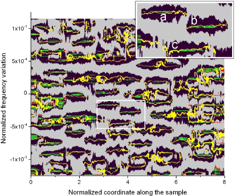
Figure 2: (color online) Mapping of $\Delta_{j}(k)$ and the normalized resonant intensities $I_{s}(j,k)$ on the coordinate-frequency plane. The units in the $x$-axis are normalized to the localization length. In the black areas $\mathrm{Re}\Delta_{j}(k)>0$, gray color corresponds to $\mathrm{Re}\Delta_{j}(k)>0$. Approximately half of the full length of any line $k=\omega/c=\mathrm{constant}$ is occupied by black areas where the cavities are located. Yellow color marks the regions where $|\arg\Delta_{j}(k)-2\pi|<0.05$. The regions with strong concentration of the wave field, where $I_{s}(j,k)>1/2$, are marked in green. As can be seen, practically all of them are located in the cavities (black areas) as predicted here. Inset: enlarged view of the selected area with three [(a), (b), and (c)] resonances.

Then, the eigenvalues, $k_{\mathrm{res}}$, have been determined from Eq. (8), and spatial distributions of the intensity created inside the samples by the incident waves with the corresponding resonant frequencies ($\omega_{\mathrm{res}}=ck_{\mathrm{res}}$) have been found and compared with the map. To facilitate this comparison, we take into account that the intensity pumped by the incident wave into a cavity depends on its location inside the sample: it decreases exponentially as the distance of the cavity from the input end increases JOSA ; Payne . As an example, the intensity distributions along the same sample illuminated by the same wave, either from the left $I_{l}(j)$ (blue curve), or from the right, $I_{l}(j)$, (red curve) ends are shown in Fig. 3a.

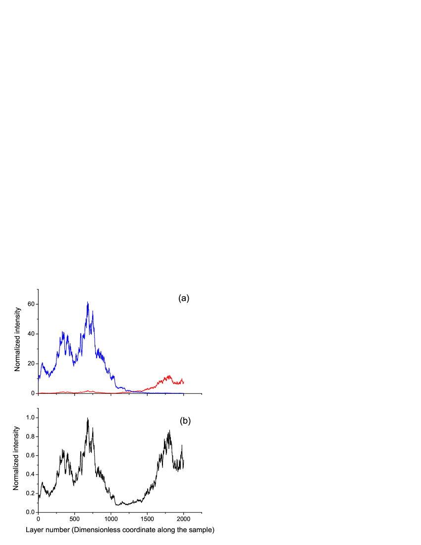
Figure 3: (color online) (a) Spatial distributions of the intensity generated by a wave incident from the left (thin blue) and right (thick red) sides of the sample; (b) intensity normalized in accordance with Eq. (19). The incident wave generates a resonance (peak of the intensity) only in the cavity closest to the edge it is coming from. The distribution of the normalized intensity is independent of the direction of incidence and clearly reveals all cavities resonant at a given frequency.

In both curves shown in Fig. 3, the intensity in the closest to the input cavity is far above the intensity inside the more distant one. Therefore we have introduced the normalized quantity

$$I_{s}(j)={\frac{\left[{I_{l}(j)\over\max\{I_{l}(j)\}}+{I_{r}(j)\over\max\{I_{r}(j)\}}\right]}{\max\left\{\left[{I_{l}(j)\over\max\{I_{l}(j)\}}+{I_{r}(j)\over\max\{I_{r}(j)\}}\right]\right\}}},$$ (19)

which is symmetric with respect to the direction of incidence and reveals equally well all resonators, independently on their positions Fig. 3b.

In Fig. 2, regions where $\mathrm{Re}\,\Delta_{j}(k)>0$ and $\mathrm{Re}\,\Delta_{j}(k)<0$ are marked by black and gray, respectively. The normalized intensity $I_{s}(j,k)$ is shown by green. Yellow color marks the regions where $|\arg\Delta_{j}(k)-2\pi|<0.05$. One can see that any horizontal cross-section $k=\mathrm{constant}$ contains approximately the same number of black and blue regions, and practically all resonances are located in “black” areas associated with cavities, as it was predicted.

Examples of the spatial distributions of $\mathrm{Re}\,\Delta_{j}$(blue curves) for three resonant frequencies marked by (a), (b), and (c) in Fig. 2 are presented in Fig. 4, along with the corresponding distributions of the intensity (red curves). Shown in Fig. 5 cross-correlation functions, $C(l)=\sum_{j}\mathrm{Re}\,\Delta_{j}I_{j-l}$, of those two types of curves reveal strong correlation between the normalized intensity and $\mathrm{Re}\,\Delta$. One can see that the cavities are well detected by the $\mathrm{Re}\,\Delta>0$ criterion.

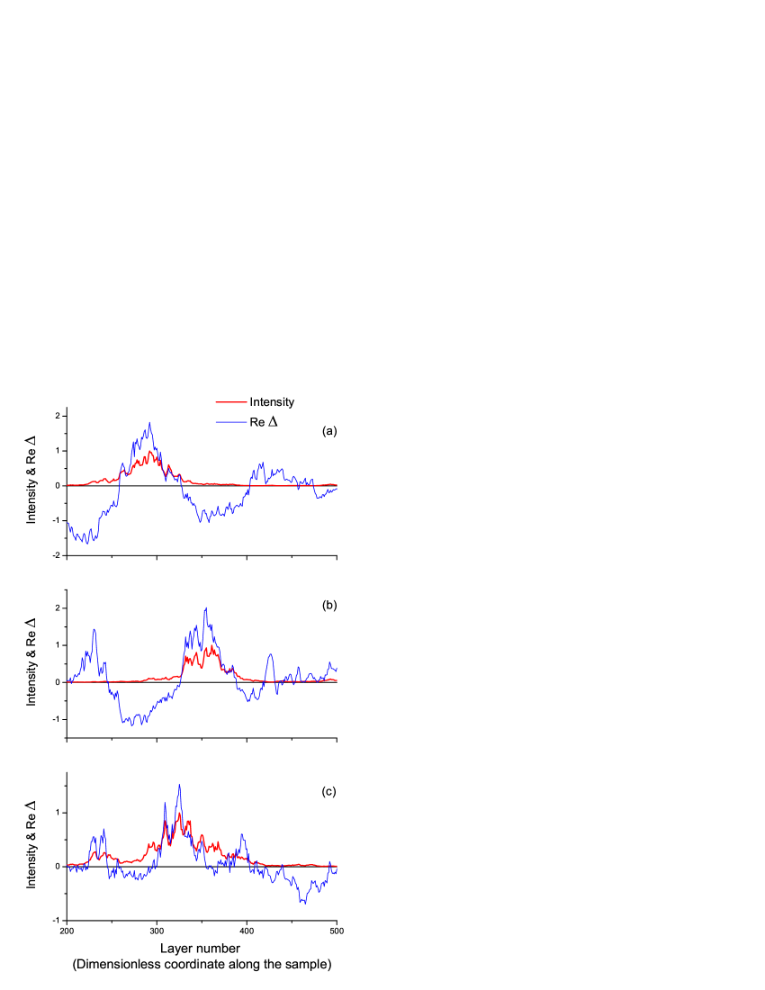
Figure 4: (color online) Spatial distributions of $\mathrm{Re}\,\Delta_{j}$ (thin blue) and of the normalized intensity (thick red) for three resonant wave numbers marked by (a), (b), and (c) in the inset in Fig. 2. One can see that each resonance is localized in the area where $\mathrm{Re}\,\Delta_{j}$ is positive and takes maximal value.

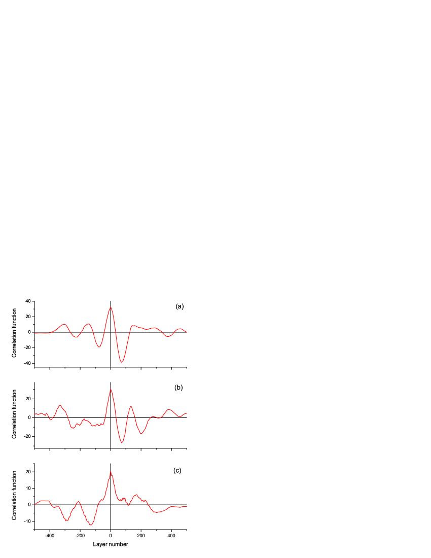
Figure 5: (color online) Cross-correlation functions $C(l)=\sum_{j}\mathrm{Re}\,\Delta_{j}I_{j-l}$ of the normalized intensity and $\mathrm{Re}\,\Delta$ for three resonant wave numbers marked by (a), (b), and (c) in the inset in Fig. 2. The curves reveal strong correlation between the normalized intensity and $\mathrm{Re}\,\Delta$.

Figure 6 demonstrates that, in accordance with Eq. (18), the number of resonances in a given frequency interval is independent of the strength of disorder (of the values of the local reflection coefficients $r_{j}$) and of the variance of the fluctuations of the thicknesses $d_{j}$, and is completely determined by the size of the sample.

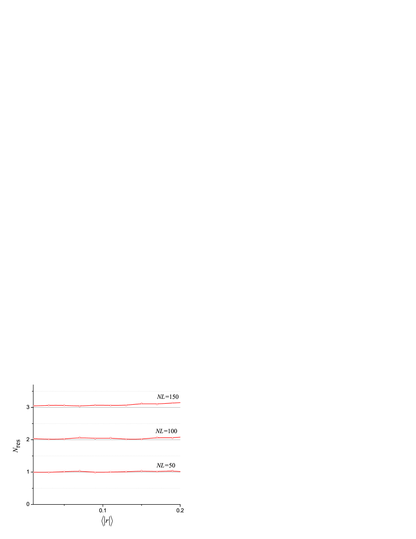
Figure 6: (color online) Number of resonances $N_{\mathrm{res}}$ as a function of the averaged local reflection coefficient (strength of disorder) $\langle|r|\rangle$. It is easy to see that, as predicted by the theory, the number of resonances in a given frequency interval grows linearly with the size of the sample and is independent of the strength of the disorder. Parameters of the numerical simulations: $k\widetilde{d}_{0}=10.0$, $\Delta k\widetilde{d}_{0}=0.1$. Each point is obtained by averaging over $10^{3}$ random samples.

This rather counter-intuitive result is also supported by the numerical simulations presented in Fig. 7, where the locations of the resonant cavities in the coordinate-frequency plane are shown (marked in black) for two samples. The samples are geometrically identical, i.e. have the same spatial distribution of the scatterers, and differ only in the amplitudes of their reflection coefficients, so that the localization length at the upper picture is twice larger than in the lower panel. When comparing both images in Fig. 7, it is easy to see that in passing from one picture to another the sizes of the black areas in the $x$-direction increase while the distances between them along the $y$-axis decrease in the same proportion, so that, in keeping with Eq. (18), $N_{\mathrm{res}}$ remains the same, meaning that there is no dependence of the number of resonances on the localization length.

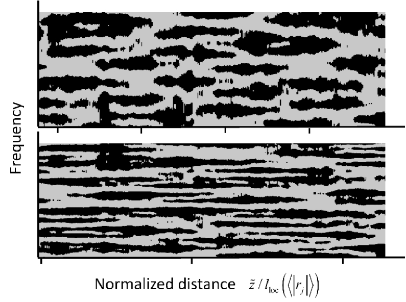
Figure 7: Distribution of the resonant cavities in the coordinate-frequency plane for two geometrically identical samples with different strengths of the scattering and thus with different localization lengths. Top: $\langle|r_{j}|\rangle=0.2$; bottom: $\langle|r_{j}|\rangle=0.15$. The distances between the black tick marks under each picture are equal to the corresponding localization lengths.

IV Experiments with active random samples: Number of lasing modes

The experimental detection of disorder-induced cavities and resonances is a challenging task in optics. Although the intensity distribution cannot be measured directly, the resonances, in principle, can be revealed by transmission experiments at different frequencies. However, although resonant transmission in lossless systems is essentially higher than at typical frequencies, it is much stronger affected by absorption, which is proportional to the exponentially large intensity inside resonators. In microwave experiments Genack we 1 ; Genack we 2 , where the absorption length was much larger than the total length of the system (single-mode waveguide), the transmission was bellow the noise level even at centrally located resonances. This fact was of little concern in that case because the microwave probe could be inserted in different points inside the waveguide. In fiber optic systems, however, this is not possible. With long optical fibers, to make the transmission measurable it might be necessary to compensate for the absorption by, for example, introducing amplification. When the amplification is sufficiently large, all resonances manifest themselves as sharp lines in the transmission spectrum.

Experimental studies of resonances in disordered optical fibers with active elements is also of interest for a better understanding of the physics of RL, because in amplifying media all resonant modes are potential candidate for lasing. The ability to monitor and to tailor their parameters, especially the total number, eigen frequencies, and locations is critical to fulfill this potential.

Random one-dimensional cavities can be created in optical fibers by the introduction of randomly-positioned reflectors, in the form of Bragg gratings 2005_Shapira . To create such structures, we have used commercial Er/Ge co-doped fibers (INO Quebec, QC, Canada) that are single-mode at 1535 nm. Erbium is the active element and germanium doping provides a kind of photosensitivity that can be used to change, locally, the refractive index. The Bragg gratings were fabricated by exposing the fiber to UV light (244 nm) from a frequency doubled argon ion laser through a periodic mask whose spatial period is 1059.8nm. Each one of the fabricated gratings had a length of approximately $5\,$mm. The random distances between the gratings were statistically independent and uniformly distributed in the interval $d_{0}\pm 0.8\,$mm, where the mean distance between gratings $d_{0}$ was approximately $5\,$mm.

The fabricated Bragg grating have a narrow reflection spectrum (its full width of half maximum is about 0.17 nm) centered at $1535.3\,$nm, with a maximum reflectivity of about 0.07-0.08. Under these conditions, the estimated localization length is found to be about 5-6 gratings. We notice that variations in the mask alignment, recording exposure, and fiber tension during the writing process caused small variations in the central wavelength of the gratings and on the sharpness of their reflection spectra. As a result, the half width of the reflection spectrum of an array of 31 gratings is about $0.27\,$nm.

The optical arrangement employed to fabricate the gratings and to measure the reflection spectra of the arrays is illustrated in Fig. 8. Laser action was obtained by end-pumping the system with 980 nm radiation from a semiconductor laser. A wavelength-division multiplexing (WDM) was used to separate the pumping wavelength from the radiation emitted by the laser (see Fig 8). Measurements of the gratings transmission/reflection coefficients with a spectral resolution of $0.001\,$nm were carried out in the spectral range $1520$–$1580\,$nm, using a tunable semiconductor laser (New Focus Velocity-6300) with a coherence length of a few meters. As illustrated in the figure, new gratings were fabricated in the sequence, beginning from the pumping end of the fiber.

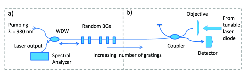
Figure 8: (color online) Schematic diagram of the experimental setup. In (a) we illustrate the configuration of the laser. The Wavelength-Division Multiplexing (WDM) device permits the separation of the pump ($980\,$nm) and lasing radiation ($1550\,$nm). In (b) we show the arrangement used to measure the reflection spectrum of the grating array during the fabrication process.

To explore the dependence of the total number of resonances, $N_{\mathrm{res}}$, on the size of the system, we measured the frequency spectrum of the reflection coefficient at samples with different numbers of reflectors, and made use of the fact that each resonance manifested itself as a sharp drop of the reflectivity. Black points in Fig. 9 represent the total number of the resonances detected in the arrays of different numbers of gratings $N_{g}$ (different lengths of the samples, $L=N_{g}d_{0}$, $d_{0}=5\,$mm) in the wavelength range ($1534.8$–$1535.6\,$nm). The theoretical prediction Eq. (18), $N_{\mathrm{res}}=1.67N_{g}$ (dotted line), is in an excellent agreement with the experimental data.

Figure 9: Top: Experimental reflection spectrum from an array of fourteen gratings. Bottom: Experimental (black points) and theoretical (dotted line) dependence of the number of resonances, $N_{\mathrm{res}}$, on the number of gratings $N_{\mathrm{g}}$. The theoretical dependence is calculated using Eq. 18 and the parameters of the experiments.

In Fig. 10, we present the results of the measurements of the emission spectra of the RL fiber containing 7, 14, 20, and 31 randomly distributed Bragg gratings (RDBG), for two values of the pumping power: 20 mW denoted by the continuous line curves, and $40\,$mW, denoted by the dashed line curves. With these pump levels, the systems were above threshold in all cases. For the measurements we used a spectrum analyzer with the resolution of $0.01\,$ nm.

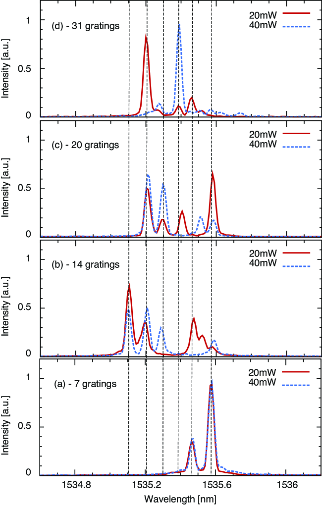
Figure 10: (color online) Emission spectra of the samples with 7, 14, 20, and 31 gratings for 20 mW (green) and 40 mW pumping powers. Both values are well above the lasing threshold. The vertical lines mark the spectral positions of the emission lines.

One can see from Fig. 10 that in the considered frequency range, the emission spectrum contains several peaks that reveal the presence of resonant modes. As the number of gratings grows so does the number of resonances: there are two peaks for the RL with seven gratings and seven peaks for the sample with 20 gratings. For the RL with seven gratings, the two peaks maintain their positions and relative intensities as the pump power increases. For systems with a higher number of gratings, the competition between modes produces temporal fluctuations in the relative strengths of the emission lines; these fluctuations also depend on the pump power. While the relative intensity of the peaks can change with the pump power, their spectral positions (indicated by the vertical lines in the figure) remain fixed.

Another interesting feature that can be observed in Fig. 10 is that, once an emission line appears in a system with a low number of gratings, it is likely to reappear in a system with a higher number of gratings. One can see, for example, that the emission lines observed with the system with seven gratings are also present in the systems with more gratings.

The curves shown in Fig 11 represent spectra of the radiation emitted by a random laser with 22 gratings, measured in 1 second intervals. Even at constant pumping power, the number of well-defined lasing modes and their emission intensity fluctuate in time. The emission frequencies, however, remain fixed; one can see that they always coincide with one of the vertical lines of the figure. The observed fluctuations of the intensity of the spectral lines could not be caused by relatively small ($\sim$5%) fluctuations of the intensity of the pumping laser, and apparently were associated with non-linear effects. Indeed, despite the relatively low power of the emission, the field inside the high-$Q$ cavities can be strong enough (due to resonance) to generate a Kerr-type nonlinearity. These effects are of importance, for example, in distributed Bragg reflector fiber lasers that are longer than $20\,$cm Lian ; Liu

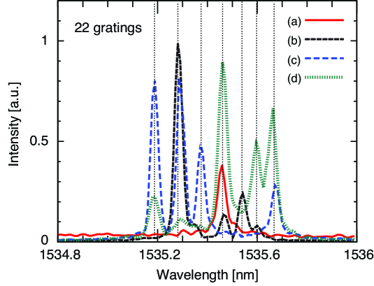
Figure 11: (color online) Emission spectra of the sample with 22 gratings generated by the fixed pumping power (40 mW) at different moments of time.

The black points in Fig. 12 denote the number of lasing modes measured in the wavelength range $\lambda\pm\Delta\lambda=1535.3\pm 0.3\,$nm in samples with different numbers of gratings $N_{g}$ (and different lengths of the system; $L=N_{g}d_{0}$, $d_{0}=5\,$mm). These numbers were obtained by adding all the emission lines present in the emission spectra over an extended period of time. The amount of the lasing modes growths linearly with the length of the system, although, in accordance with the theoretical reasoning above, it is always less than the total number of the effective resonant cavities in the sample (Fig. 9).

Figure 12: Number of resonances measured in the wavelength range $\lambda\pm\Delta\lambda=1.5\cdot 10^{-4}\pm 0.85\cdot 10^{-8}$cm (black points) as a function of the number of Bragg reflectors. Since the total length of the sample is proportional to the number of gratings, the figure actually presents the dependence on size of the random system.

V Summary

To conclude, eigen-modes (resonances) of a randomly layered long ($L\gg l_{\mathrm{loc}}$) sample are localized in disorder-induced effective cavities of the size of the order of the localization length that are randomly distributed along the sample. An algorithm for finding this distribution in an individual configuration with arbitrary (random) parameters was developed based on the calculation of the function $\Delta_{j}(k)$ in Eq. (7). It was shown that a cavity of an effective size of a few localization lengths, in which a mode with $k=k_{\mathrm{res}}$ can be localized, exists around $j$-th layer when $\mathrm{Im}\,\Delta_{j}(k_{\mathrm{res}})=0$ and $\mathrm{Re}\,\Delta_{j}(k_{\mathrm{res}})>0.$ In the case of uncorrelated disorder and weak scattering, the spacing between eigen-levels and the number of cavities $N_{\mathrm{res}}$ in a given frequency interval does not depend on the strength of disorder, and are uniquely determined by the size of the sample. The frequency of each resonance is independent of the coordinate of the effective cavity, in which it is located. The number of lasing modes depends also on the ratio between the threshold values $g_{c}^{(j)}$ of the individual cavities and the gain $g$ of the medium, and is less than $N_{\mathrm{res}}$. The theoretical predictions and numerical results are in reasonable agreement with the experimental data obtained by measuring the emission spectra of the random laser based on the single-mode fiber with randomly distributed Bragg gratings.

.