Quantum star-graph analogues

of ${\cal PT}-$symmetric square wells

Miloslav Znojil

Nuclear Physics Institute ASCR,

250 68 Řež, Czech Republic

e-mail: znojil@ujf.cas.cz

Abstract

Non-Hermitian ${\cal PT}-$symmetric Hamiltonians $H=-d^{2}/dx^{2}+V(x)$ with $x\in\mathbb{R}$ are reinterpreted as describing the most elementary phenomenological quantum graph, i.e., a system living on the two half-line edges connected at a single matching-point vertex in the origin. A $q-$pointed star graph generalization of these $q=2$ models is then proposed and studied. For a special toy-model point interaction yielding the exactly solvable model at $q=2$, the bound-state energies are finally identified with the roots of a remarkably compact trigonometric function at any $q=2,3,\ldots$.

PACS

03.65.Ca Formalism

03.65.Db Functional analytical methods

03.65.Ta Foundations of quantum mechanics; measurement theory

03.70.+k Theory of quantized fields

1 Introduction

The heuristic use of the concept of ${\cal PT}$ symmetry, i.e., of the parity-times-time-reversal symmetry of quantum Hamiltonians $H$ and/or of the toy-model wave functions $\psi(x)$ (with, say, $x\in\mathbb{R}$) proved unexpectedly productive in phenomenologically oriented quantum field theory [1, 2] or in the context of relativistic quantum mechanics [3, 4], in the supersymmetric model-building [5, 6] or, recently, in experimental classical optics [7].

One of the simplest illustrative examples of a ${\cal PT}$ symmetric Hamiltonian has been proposed in Ref. [8]. In the model the quantum motion remained free inside a finite interval of coordinates,

$$-\frac{d^{2}}{dx^{2}}\Psi(x)=E\,\Psi(x)\,,\ \ \ \ \ \ \ x\in(-L,L)\,.$$ (1)

The only dynamical information has been carried by the very specific point interaction induced by the external Robin-type boundary conditions containing the single real coupling constant $\alpha$,

$$\Psi^{\prime}(\pm L)+i\alpha\;\!\Psi(\pm L)=0\,,\ \ \ \ \alpha>0\,.$$ (2)

This dynamical input yielded the phenomenology-oriented real bound-state spectrum

$$E_{0}=\alpha^{2}\,,\ \ \ E_{n}=\left(\frac{n\pi}{2L}\right)^{2}\,,\ \ \ n=1,2,\ldots\,.$$ (3)

Its explicit form enabled us to restrict our attention, for the sake of simplicity, to the non-degenerate systems where $2L\alpha/\pi\neq 1,2,\ldots$. The probabilistic quantum-mechanical interpretation of the closed-form wave functions of the model also appeared feasible. The explicit formulae yielding the unitary forms of the model (i.e., in the notation of review [9], all of the non-equivalent “standard” inner-product representations of the eligible physical Hilbert space of states ${\cal H}^{(S)}$) were found and described in a series of mathematically rigorous subsequent studies [10, 11].

The appealing and, in some sense, extreme simplicity of the latter exceptional model inspired, naturally, a number of generalizations (cf., e.g., Refs. [11, 12]). Also our present paper will describe a new generalization of the model.

2 A quantum-graph reinterpretation of the ${\cal PT}-$symmetric square-well models

A formal core of our present considerations will lie in the reinterpretation of Eq. (1) where the interval of $x\in(-L,L)$ will be treated as a union $\mathbb{G}^{(2)}$ of a pair of equal-length subintervals (or “edges”) $e_{+}=(0,L)$ and $e_{-}=(-L,0)$ forming an elementary “graph” with the single “vertex” at $x=0$.

In such a case it is necessary to distinguish between the theoretical and purely phenomenological informal aspects of such a reinterpretation. Indeed, the latter, “realistic” aspect is very natural. Traditionally, it finds its widespread use in quantum chemistry where, typically, the valence electron of an organic molecule may be often treated as moving just strictly along the atomic-bond edges [13].

In the former, more abstract and less phenomenological setting the restriction of the motion to the edges of a suitable graph may enormously simplify the underlying Schrödinger equation [14]. Recently, this idea made the study of various quantum-graph models extremely popular. Pars pro toto the interested reader may be recommended to consult a comprehensive collection [15] of more than 700 pages of reviews and original research reports, with the scope ranging from certain entirely “unrealistic” scenarios (i.e., e.g., from the fractal and/or chaos-simulating graphs [16]) down to certain very realistic models of observable photonic crystals and various other “leaky-graph” nanostructures encountered, typically, in condensed matter physics [17].

For the sake of definiteness, let us now assume that in our above most elementary graph $\mathbb{G}^{(2)}$, both of the respective edges are oriented inwards, i.e., $e_{\pm}=e_{\pm}(y_{\pm})$ with $y_{+}=L-x\in(0,L)$ while $y_{-}=L+x\in(0,L)$. Without any real loss of generality, our attention will also remain restricted to the dynamics represented by the end-point point interaction as mediated by boundary conditions (2).

In the new notation we have to replace Eq. (1) by the pair of differential Schrödinger equations

$$-\frac{d^{2}}{dy_{\pm}^{2}}\psi_{\pm}(y_{\pm})=E\,\psi_{\pm}(y_{\pm})\,,\ \ \ \ \ \ \ y_{\pm}\in(0,L)\,$$ (4)

complemented by the standard regular matching conditions in the origin,

$$\psi_{+}(L)=\psi_{-}(L)\,,\ \ \ \ \ \ \partial_{y_{+}}\psi_{+}(L)+\partial_{y_{-}}\psi_{-}(L)=0\,.\,$$ (5)

The external Robin-type boundary conditions (2) must now read, mutatis mutandis,

$$\psi^{\prime}_{\pm}(0)=\pm i\alpha\;\!\psi_{\pm}(0)\,.$$ (6)

The physics (i.e., the spectrum) remains unchanged but the mathematical meaning of the ${\cal PT}-$symmetry of $H$ (i.e., the representation of the antilinear operator $\omega={\cal PT}$) gets modified.

2.1 Operators of symmetries

After the change of the language, the differential-operator Hamiltonian (originally defined as acting, in general, in $L^{2}(\mathbb{R})$) must be treated as acting in another, “friendly” [9] Hilbert space of states ${\cal H}^{(F)}=L^{2}(\mathbb{R}^{+})\bigoplus L^{2}(\mathbb{R}^{+})$. Formally, Schrödinger Eq. (4) then acquires the two-by-two operator-matrix form

$$\left(\begin{array}[]{cc}H_{+}-E&0\\ 0&H_{-}-E\end{array}\right)\left(\begin{array}[]{c}\psi_{+}\\ \psi_{-}\end{array}\right)=0\,$$ (7)

(i.e., $(H-EI)|\psi\rangle=0$ in an abbreviated notation).

The original linear operator of parity ${\cal P}$ (i.e., the reflection which changed the sign of the coordinate, ${\cal P}:x\to-x$, $x\in(-L,L)$) will now play the slightly different role of a domain-intertwiner such that ${\cal P}:y_{\pm}\to y_{\mp}$, i.e.,

$${\cal P}=\left(\begin{array}[]{cc}0&I\\ I&0\end{array}\right)\,.$$ (8)

The parallel interpretation of the antilinear symmetry $\omega={\cal PT}$ of $H$ will vary with the spectral properties of $H$ [18]. As long as we may define $|\psi^{\prime}\rangle=\omega|\psi\rangle$, we may write $\omega(H-EI)|\psi\rangle=(H-E^{*}I)|\psi^{\prime}\rangle=0$. Thus, in the generic non-degenerate case we must distinguish between the real-energy scenario $E=E^{*}$ (in which $|\psi^{\prime}\rangle$ will be proportional to $|\psi\rangle$) and the case of $E\neq E^{*}$ in which the two eigenvectors $|\psi^{\prime}\rangle$ and $|\psi\rangle$ of $H$ remain linearly independent (or, in the language of wave functions, in which the ${\cal PT}$ symmetry becomes spontaneously broken [2]).

2.2 Wave functions and energies

In the case of the unbroken ${\cal PT}$ symmetry we may always change the phase of the initial ket vector $|\psi\rangle$ in such a way that $|\psi^{\prime}\rangle=|\psi\rangle$. In the original $L^{2}(\mathbb{R})$ context this was a normalization convention in which both the respective symmetric and antisymmetric components of $\Psi(x)=S(x)+{\rm i}A(x)$ with properties $S(-x)=S(x)$ and $A(-x)=-A(x)$ were real.

In the current literature, people sometimes speak about the ${\cal PT}$ symmetry of the system while tacitly assuming that it is not spontaneously broken, i.e., that the spectrum is real and non-degenerate. Under such an assumption it is rather straightforward to return to our specific model and to write down the definitions of the two new wave functions $\psi_{\pm}(y_{\pm})$ with $y_{\pm}\in(0,L)$ in terms of the components of the old wave function $\Psi(x)$,

$$\psi_{-}(y_{-})=S(L-y_{-})-{\rm i}A(L-y_{-})\,,\ \ \ \ \ \ \psi_{+}(y_{+})=S(L-y_{+})+{\rm i}A(L-y_{+})\,.$$ (9)

This formula confirms that the time reversal operator ${\cal T}$ itself acts, as usual, as complex conjugation.

In the new notation the general solution of differential Eq. (4)

$$\psi_{\pm}(y)=A_{\pm}\,\sin ky+B_{\pm}\,\cos ky\,$$ (10)

must be restricted, first of all, by the external boundary conditions at $y=0$. This yields the rule

$$k\,A_{\pm}=\pm{\rm i}\alpha B_{\pm}\,.$$ (11)

Its insertion in Eq. (10) defines the wave functions. Finally, the necessity of their matching in the central vertex, i.e., relation

$$\frac{k\,\tan kL-{\rm i}\alpha}{k+{\rm i}\,\alpha\tan kL}+\frac{k\,\tan kL+{\rm i}\alpha}{k-{\rm i}\,\alpha\tan kL}=0\,\,$$ (12)

leads to the ultimate secular equation

$$2\,\,\frac{k^{2}-\alpha^{2}}{k^{2}+\alpha^{2}\,\tan^{2}kL}\tan kL=0\,.$$ (13)

Although this equation looks different from the secular equation as given in Ref. [8] (where one merely has to set $d=2\,L$ in eqs. Nr. 13 and 14), the set of the resulting energy roots (3) remains the same of course. It is worth noticing that from our present form of secular equation (13) the complete set of eigenvalues is determined via zeros of a triplet of elementary functions $f_{1}(k):=k^{2}-\alpha^{2}$, $f_{2}(k):=\tan kL$ and $f_{3}(k):={\rm cotan}\,kL$.

3 The new model with $q$ equilateral edges

In the above-introduced notation the generalization of the model becomes straightforward. At any $q\geq 2$ we merely consider a $q-$plet of Schrödinger equations

$$-\frac{d^{2}}{dy_{j}^{2}}\psi_{j}(y_{j})=E\,\psi_{j}(y_{j})\,,\ \ \ \ \ \ \ y_{j}\in(0,L)\,,\ \ \ \ \ j=0,1,\ldots,q-1$$ (14)

for which the $q-$plet of edges $e_{j}=e_{j}(y_{j})$ with $y_{j}\in(0,L)$ may be visualized as forming a star-shaped graph $\mathbb{G}^{(q)}$ with the single central vertex at $y_{j}=L$. For the sake of simplicity, the matching in the origin will be chosen in the elementary Kirchhoff’s form

$$\psi_{j}(L)=\psi_{0}(L)\,,\ \ \ \ j=1,2,\ldots,q-1\,,\ \ \ \ \ \ \ \sum_{j=0}^{q-1}\,\partial_{y_{j}}\psi_{j}(L)=0\,.$$ (15)

In a completion of the tentative analogy, the complex rotation by angle $\pi$ as used in Eq. (6) will be replaced now by the complex rotation by an appropriate fractional angle $\phi=\phi(q)=2\pi/q$, yielding the prescription

$$\partial_{x_{j}}\psi_{j}(0)=i\alpha\,e^{{\rm i}j\varphi}\,\psi_{j}(0)\,,\ \ \ \ \ j=0,1,\ldots,q-1\,,\ \ \ \varphi=2\pi/q\,.$$ (16)

3.1 Wave functions

The general solution of the differential Schrödinger system (14)

$$\psi_{j}(x)=A_{j}\,\sin kx+B_{j}\,\cos kx\,,\ \ \ \ j=0,1,\ldots,q-1$$ (17)

yields also the auxiliary expression for the derivatives,

$$\partial_{x}\,\psi_{j}(x)=k\,A_{j}\,\cos kx-k\,B_{j}\,\sin kx\,,\ \ \ \ j=0,1,\ldots,q-1\,.$$ (18)

One converts the dynamical boundary conditions (16) into an elementary connection between coefficients,

$$k\,A_{j}=i\alpha\,e^{{\rm i}j\varphi}\,B_{j}\,,\ \ \ \ \ j=0,1,\ldots,q-1\,,\ \ \ \varphi=2\pi/q\,.$$ (19)

The continuity condition for wave functions in the central vertex

$$\left[i\alpha\,e^{{\rm i}j\varphi}\,\sin kL+k\,\cos kL\right]\,B_{j}=k\,\varrho\,,\ \ \ \ j=0,1,\ldots,q-1\,$$ (20)

enables us to define all of the coefficients $B_{j}=B_{j}(\varrho,L,k)$ as proportional to the auxiliary parameter $\varrho$. Their subsequent insertion in the explicit version

$$\sum_{j=0}^{q-1}\,\left[i\alpha\,e^{{\rm i}j\varphi}\,\cos kL-k\,\sin kL\,\right]\,B_{j}=0\,$$ (21)

of the Kirchhoff’s law of Eq. (15) finally leads to a rather complicated trigonometric secular equation which defines, in principle at least, all of the bound-state energies $E=E_{n}$. As long as the underlying Hamiltonian is non-Hermitian, these energies may be both real and complex at $q>2$. Some of them also need not remain expressible via any closed-form analogue of the special $q=2$ formula (3).

3.2 Secular equation

After the elimination of $B_{j}$s the secular equation for bound-state energies $E=k^{2}$ acquires a compactified form

$$\sum_{j=0}^{q-1}\,\tan\left[kL-\beta_{j}(k)\right]=0\,\,$$ (22)

where the parameter $\varrho$ dropped out and where we defined, implicitly,

$$\tan\beta_{j}(k)=\frac{{\rm i}\alpha\,\exp({{\rm i}j\varphi})}{k}=C+{\rm i}K\,,\ \ \ \ j=0,1,\ldots,q-1\,,\ \ \ \varphi=2\pi/q\,.$$

Setting $\beta_{j}=u+{\rm i}v$ we may abbreviate $\tan u=U$ and $\tanh v=V$ and write

$$\tan\beta_{j}=\frac{U+{\rm i}V}{1-{\rm i}UV}=\frac{(U+{\rm i}V)(1+{\rm i}UV)}{1+U^{2}V^{2}}=\frac{U(1-V^{2})+{\rm i}V(1+U^{2})}{1+U^{2}V^{2}}\,.$$

As long as

$$C=C(j,k)=-\frac{\alpha}{k}\,\sin j\varphi\,,\ \ \ \ \ \ K=K(j,k)=\frac{\alpha}{k}\cos j\varphi\,$$

we obtain the real-function correspondences

$$C(j,k)=\frac{\sin u\cos u}{\cos^{2}u+\sinh^{2}v}\,,\ \ \ \ K(j,k)=\frac{\sinh v\cosh v}{\sinh^{2}v+\cos^{2}u}\,$$

as well as the closed-form inversion formulae

$$\tan j\varphi=\frac{\sin 2u}{\sinh 2v}\ \left(\,=\frac{C}{K}\right)\,,\ \ \ \ \ \frac{\alpha^{2}}{k^{2}}=\frac{\sinh^{2}v+\sin^{2}u}{\sinh^{2}v+\cos^{2}u}\ \left(\,=C^{2}+K^{2}\right)\,.$$

From the latter relation we may finally eliminate $\sinh v$ and convert the former relation into an easily solvable quadratic equation for the value of $\cos^{2}u$, yielding the two eligible roots as functions of $j$ and $k$.

In this manner, secular equation (22) would be given a lengthy and rather clumsy but still explicit elementary form which we are not going to display here of course. Anyhow, at any pair of given parameters $q$ and $\alpha$ the whole eigenvalue problem may be now solved, numerically, with arbitrary precision.

4 Secular equation revisited

Let us now demonstrate that for the purposes of symbolic-manipulation simplifications, secular Eq. (22) should be reconsidered in the apparently more complicated form of the sum

$$\sum_{j=0}^{q-1}\,\frac{\tan kL-C(j,k)-{\rm i}K(j,k)}{1+[C(j,k)+{\rm i}K(j,k)]\,\tan kL}=0\,.\,$$ (23)

In what follows we are now going to show that and how the simplification of this formula may be achieved by the explicit summation when proceeding, in a systematic inductive manner, from the smallest integers $q$ upwards.

4.1 The trivial single-line quantum graph: $q=2$.

At $q=2$ we have $\tan\beta_{0,1}(k)=\pm{\rm i}\alpha/k$ so that one obtains $C(j,k)=0$ and $K(\{0,1\},k)=\pm\alpha/k$. This makes secular equation (23) reducible to the ultimate elementary constraint (13).

4.2 The three-pointed star graph

When we abbreviate $\gamma=\alpha/2$, the $q=3$ three-term secular equation

$$\frac{k\,\tan kL-2{\rm i}\gamma}{k+2{\rm i}\,\gamma\tan kL}+\frac{k\,\tan kL+\gamma\,\sqrt{3}+{\rm i}\gamma}{k-({\rm i}+\sqrt{3})\,\gamma\tan kL}+\frac{k\,\tan kL-\gamma\,\sqrt{3}+{\rm i}\gamma}{k-({\rm i}-\sqrt{3})\,\gamma\tan kL}=0\,\,$$ (24)

may be rewritten in its simplified, single-term form

$$3\,\frac{k^{3}+{\rm i}\alpha^{3}\,\tan kL}{k^{3}-{\rm i}\,\alpha^{3}\tan^{3}kL}\,\tan kL=0\,.\,$$ (25)

The inspection of this secular equation reveals that the real and discrete part of the $q=3$ bound-state spectrum coincides with its $q=2$ predecessor, up to the anomalous root $k=\alpha$ which now disappeared. In other words, the real roots of the new secular Eq. (25) coincide now strictly with the zeros of the real functions $\tan kL$ and ${\rm cotan}\,kL$.

It is necessary to add that our secular Eq. (25) also possesses complex roots defined by subcondition

$$k^{3}+{\rm i}\alpha^{3}\,\tan kL=0\,.\,$$ (26)

We may decompose ${k}/{\alpha}=\mu+{\rm i}\nu$, set $\lambda=\alpha\,L$ and obtain the complex version of such a secular subequation

$$\mu^{3}-3\,\mu\,\nu^{2}+{\rm i}\left(3\,\mu^{2}\nu-\nu^{3}\right)=\frac{\tan\mu\lambda+{\rm i}\,\tanh\nu\lambda}{1-{\rm i}\tan\mu\lambda\,\tanh\nu\lambda}$$

which is equivalent to the coupled pair of the real secular subequations

$$\mu^{3}-3\,\mu\,\nu^{2}+\left(3\,\mu^{2}\nu-\nu^{3}-1/\tanh\nu\lambda\right)\,\tan\mu\lambda\,\tanh\nu\lambda=0$$

and

$$3\,\mu^{2}\nu-\nu^{3}-\tanh\nu\lambda-\left(\mu^{3}-3\,\mu\,\nu^{2}\right)\,\tan\mu\lambda\,\tanh\nu\lambda=0\,.$$

In an extensive numerical test we revealed and demonstrated the existence of nontrivial complex roots of these equations at the various values of $\lambda$. For example, we localized the sample pair of roots with $\mu=1.20484$ and $\nu=\pm 0.3507$ at $\lambda=1$. This means that at $q=3$ the non-Hermiticity of the Hamiltonian may probably be interpreted as “too strong”. In other words, the Hamiltonian of the quantum version of this system cannot be Hermitized using just the standard techniques as reviewed in Ref. [9], at any coupling constant $\lambda$.

In this sense, the practical phenomenological applicability of our $q=3$ quantum graph appears restricted to the domain of non-linear optics [7] and to the various similar, recently popular classical-physics (or even classical-mechanics [19]) implementations and applications of the theory where the complex energies may and do find their natural physical interpretation.

Naturally, the situation is different in quantum physics where, inside the physical Hilbert space ${\cal H}$, the spectrum of any operator $H$ representing an observable quantity must be real. Still, there exists a certain recently discovered [20] space-projection trick which may prove acceptable in at least some phenomenological considerations and applications of our models.

4.3 Quantum-Hilbert-space construction at $q=3$

We just demonstrated, constructively, that the discrete energy spectrum of at least some of our present $q>2$ quantum-graph models need not necessarily be all real. In all of these “non-real-spectrum” cases it seems necessary to discard the underlying Hamiltonian $H=H^{(q)}(\alpha)$ as leading to non-unitary evolution of the quantum system in question. At the same time, many of the formal (e.g., solvability) as well as phenomenological (e.g., scattering-related [21]) features of these and similar models might seem appealing enough. For this reason, let us now describe, briefly, one of the recently discovered and more or less universal remedies of the apparent complex-energy shortcoming.

Firstly, let us remind the readers that within the rigorous quantum theories one must often exclude all of the non-Hermitian Hamiltonians $H$ (leading to the real spectrum or not) which cannot be assigned a suitable Hilbert space in which they may be reinterpreted (typically, via a suitable inner product [2, 9]) as self-adjoint. In particular, this year it has been proved [22] that in this manner it would be even necessary to discard the popular imaginary cubic oscillator and many other standard benchmark ${\cal PT}-$symmetric quantum models with real spectra.

Naturally, this conclusion may seem rather surprising. Unfortunately, it is based on the rigorous functional analysis and, hence, mathematically valid. The essence of the apparent paradox has been found in the inconsistency between the a priori choice of the same domain ${\cal D}$ of $H$ before and after the Hermitization, ${\cal D}^{\rm(before)}(H)={\cal D}^{\rm(after)}(H)$.

This conclusion may be perceived as indication of the way out of the trap. Indeed, a physics-oriented and pragmatic (thought still mathematically rigorous) way out of such a form of crisis of the theory has been found, almost in parallel, in Ref. [20]. In a simplified explanation it has been merely admitted that ${\cal D}^{\rm(before)}(H)\neq{\cal D}^{\rm(after)}(H)$.

The resulting flexibility of the “projection” on the meaningful vector space ${\cal D}^{\rm(after)}(H)$ of the correct physical states enables us to construct the latter space simply as spanned by any subset of the eigenvectors of the Hamiltonian $H$ in question. In other words, the formal recipe as presented in Ref. [20] may be simply read as just another version of the innovative implementation of the abstract principles of quantum theory where the correct Hilbert space ${\cal H}$ is determined dynamically (plus, in the present case, in the mere real-energy subspace).

Once we return now to our present specific $q=3$ quantum-graph Hamiltonian $H$ where we choose, a priori, the usual and friendly (but, in general, unphysical) Hilbert-space domain ${\cal D}^{\rm(before)}(H)=\bigoplus_{j=0}^{2}\,L^{2}(e_{j})$ (in this space, $H\neq H^{\dagger}$ of course), we may now use just the slightly adapted recipe of Ref. [20]. Thus, in essence, we have to construct the correct vector space ${\cal D}^{\rm(after)}(H)$ (as well as its bra-vector dual) as spanned just by the real-eigenvalue eigenvectors of $H$ (or of $H^{\dagger}$, respectively).

We omit the further details here, summarizing that due to the infinite number of the real eigenvalues at our disposal, the dimension of ${\cal D}^{\rm(after)}(H)$ will remain infinite. The immanent projector-operator nature of the whole construction may, indeed, be perceived as far from trivial, with details lying, certainly, far beyond of the scope of our present paper. Thus, we may only add that although, in the projected-space approach, the subsequent Hermitization of the model remains entirely routine [9], the physical interpretation or our star-shaped-graph models remains the same as in the most elementary $q=2$ special case. For this reason, some of the apparent paradoxes (like, e.g., the intrinsically non-local nature of the well known $q=2$ system [21]) will survive the transition to $q>2$ of course.

4.4 Secular equation at $q=4$

The $q=4$ version of our secular equation reads

$$\frac{k\,\tan kL-{\rm i}\alpha}{k+{\rm i}\,\alpha\tan kL}+\frac{k\,\tan kL+{\rm i}\alpha}{k-{\rm i}\,\alpha\tan kL}+\frac{k\,\tan kL-\alpha}{k+\alpha\tan kL}+\frac{k\,\tan kL+\alpha}{k-\,\alpha\tan kL}=0\,\,$$ (27)

and may be again simplified,

$$4\,\frac{k^{4}+\alpha^{4}\,\tan^{2}kL}{k^{4}-\alpha^{4}\tan^{4}kL}\,\tan kL=0\,.\,$$ (28)

The real stable-bound-state spectrum remains the same as at $q=3$. The complex roots of the auxiliary subequation $k^{4}+\alpha^{4}\,\tan^{2}kL=0$, i.e., of the two equations $k^{2}=\pm{\rm i}\alpha^{2}\,\tan kL$ related by the formal change of $k\to-k$ may be sought just in a half-plane of complex $k$. The final analysis of this equation may again proceed in the manner outlined in preceding subsection.

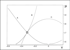
Figure 1: Numerical identification of a complex root of secular equation.

Once we make a particular choice of the sign (say, plus), we obtain the simplest special case of the equation for the complex roots $k=\mu+{\rm i}\,\nu$. In units $L=1$ we have

$$\mu^{2}-\nu^{2}+2\,{\rm i}\,\mu\nu=+{\rm i}\,\alpha^{2}\,\tan(\mu+{\rm i}\,\nu)\,.$$ (29)

This is a complex equation which decays into the pair of real conditions

$$\mu^{2}-\nu^{2}+2\,\mu\nu\,\tan\mu\,\tanh\nu+\alpha^{2}\,\tanh\nu=0\,,$$ (30)

$$2\,\mu\nu-(\mu^{2}-\nu^{2})\,\tan\mu\,\tanh\nu-\alpha^{2}\,\tan\mu=0\,.$$ (31)

The search for a nontrivial root of these two equations remains numerical. Figure 1 samples the localization of a complex root $k=\sqrt{E}$ with components $\mu\approx 1.7025$ and $\nu\approx-0.3165$ at $\alpha=1$.

Let us add that the efficiency as well as the reliability of the latter search for a complex root was significantly enhanced by a trick in which the two real equations (30) and (31) (defining, in our illustrative picture, curves A and B in the $\mu-\nu$ plane, respectively) were complemented by the third, redundant rule of the coincidence of the absolute values of the left- and right-hand side of the complex relation $k^{2}=\pm{\rm i}\alpha^{2}\,\tan k$,

$$\mu^{2}+\nu^{2}=\alpha^{2}\,\sqrt{\frac{\tan^{2}\mu+\tanh^{2}\nu}{1+\tan^{2}\mu\,\tanh^{2}\nu}}\,.$$ (32)

In our picture this defines the redundant, additional curve $C$ in the $\mu-\nu$ plane. We see that its construction helps us to identify the root in question via a triple intersection of the curves A, B and C. Naturally, such a recipe keeps the numerical errors under a very reliable control.

4.5 Secular equation at $q=5$

At $q=5$ our secular equation becomes perceivably more complicated but the use of computerized symbolic manipulations and appropriate trigonometric identities is still found to lead to the thoroughly simplified prescription

$$5\,\frac{k^{5}-{\rm i}\alpha^{5}\,\tan^{3}kL}{k^{5}+{\rm i}\alpha^{5}\tan^{5}kL}\,\tan kL=0\,,\ \ \ \ \ q=5\,.$$ (33)

This formula indicates that the real part of the spectrum remains unchanged also at $q=5$. On the more important methodical level the structure of this formula confirms our expectation that the sum (23) may be represented by a very simple function of $q$.

4.6 Secular equation at any $q$

On the basis of the above particular results yielding the explicit and elementary closed summation formulae it is straightforward to conjecture and prove the validity of the following extrapolated general trigonometric secular equation

$$q\,\frac{k^{q}+({\rm i}\alpha)^{q}\,\tan^{q-2}kL}{k^{q}-({\rm i}\alpha)^{q}\tan^{q}kL}\,\tan kL=0\,,\ \ \ \ \ q=2,3,\ldots\,.$$ (34)

Whenever we restrict our attention just to the real roots $k$ which correspond to the stable bound-state solutions, we reveal that the numerator in the fractional part of the left-hand-side secular determinant (34) plays now the role of the source of the $q>2$ analogues of the single anomalous $q=2$ root $k=\alpha$.

This numerator cannot vanish at real $k$ and odd $q=2m+1$, $m\in\mathbb{Z}^{+}$ and it cannot vanish at $q=4m$, $m\in\mathbb{Z}^{+}$, either. The remaining values of the integer $q={4m-2}$, $m\in\mathbb{Z}^{+}$ appear exceptional. Their choice leads to the emergence of the additional real zeros and so it deserves a separate attention.

4.7 Secular equation at the exceptional $q=4m-2$

At $q=2$ our quantum-graph spectrum was all real (cf. sec. 4.1 above) but, as we saw, the situation became anomalous at any $q\geq 3$. Nevertheless, what is new at the exceptional integers $q=4m-2$, $m=2,3,\ldots$ is that the secular-equation factor

$$k^{4m-2}-\alpha^{4m-2}\,\tan^{{4m-4}}kL=0\,$$ (35)

becomes nontrivial and, moreover, that it produces, obviously, certain potentially real additional bound-state eigenvalues $E=k^{2}$.

One of the unfortunate consequences of the latter observation is that some of the energies of the stable quantum-star bound states cease to be obtainable in closed form. Their determination must be performed by suitable brute-force numerical methods. Moreover, the practical search for the roots of transcendental Eq. (35) or of its slightly more friendly and graphically better tractable version

$$k_{anomalous}=\alpha\,\tan^{1-1/(2m-1)}k_{anomalous}L=0\,,\ \ \ \ \ m=1,2,\ldots\,$$ (36)

becomes technically complicated. A priori, without any extensive calculations we can immediately be sure that at the sufficiently small $\alpha$s, all of the generic and $m-$independent real roots $k=(n+1/2)\pi\gg 1$ with $n=0,1,\ldots$ become accompanied by the neighboring real pairs of eigenvalues which are produced by Eq. (36).

With the growth of $\alpha$ this picture will first lose its validity between $k=0$ and $k=\pi/2$. At the sufficiently small $\alpha$s one always finds there the two smallest real roots inside the interval. With the growth of parameter $\alpha$ these two roots move towards each other at a speed which depends on $m$. In a numerical experiment performed at $m=2$ we found that there exists the critical value of $\alpha=\alpha_{critical}\approx 0.7863$ at which these two lowest anomalous energy-level twins merge at $k\approx 0.748$ and, subsequently, complexify.

This observation may only be read as a reliable numerical proof that at the sufficiently large values of the strength of the non-Hermiticity $\alpha>\alpha_{critical}$ (with $\alpha_{critical}\approx 0.7863$ at $m=2$), the spectrum of the whole system certainly contains non-real eigenvalues.

In the interval of $\alpha<0.7863$ we may only conclude that there exists a set of certain new and strictly real “anomalous” eigenvalues which may only be generated numerically (i.e., say, via our secular sub-equation (36)). This extremely interesting infinite family of the new quantum states is, in principle, observable. Its energy levels (which form, incidentally, almost degenerate pairs at higher excitations) may be interpreted as the appropriate quantum-graph $q=6$, $q=10$ (etc) analogues of their single-state $q=2$ predecessor $E_{0}(\alpha)$ of Eq. (3).

5 Summary

In our preceding papers [23, 24] on ${\cal PT}-$symmetric quantum graphs we always restricted our attention to their mere discrete approximants. In our present paper, we abandoned this approach as not sufficiently efficient. An alternative way of circumventing the technical obstacles has been found here in an ad hoc restriction of the class of the admissible graphs to their star-shaped subset $\mathbb{G}^{(q)}$. Due to this restriction, we were able to replace the universal though less powerful discretization approach by the much more elementary method of matching of wave functions at the central vertex.

In technical sense, our present results may be perceived as a return to optimism. The main source of the simplification of our constructive considerations may be identified with the inherent symmetry of the complex Robin boundary conditions. This symmetry found its fructification in the emergence of powerful trigonometric identities. These identities led to the enormous simplification of the related secular equations at any integer $q\geq 2$. In this sense one could find here certain parallels with the role of trigonometric identities, say, during the early stages of development of Calogero models [25] and/or of some of their less influential analogues [26].

The transition to nontrivial topology of the graph-related phase space (or of the space of coordinates) manifested itself in two ways. Firstly, a part of the physical sector where the bound-state energies remained strictly real appeared independent of the number of rays $q$, i.e., mathematically stable. Secondly, strictly this part of the spectrum also remained defined by closed formulae at $q>2$. In contrast, the rest of the spectrum (and, in particular, the whole sector of “resonances” where the energies are complex) appeared changing with the changes of $q$.

Due to the elementary form of the secular equations at any $q$, the “friendly” closed-form real energies coincided with their elementary square-well $q=2$ predecessors. In contrast, it appeared rather difficult to localize the precise position of all of the complex bound-state energies in complex plane. A sophisticated numerical approach appeared necessary for the purpose.

In the context of physics the potential phenomenological applicability of our present family of toy-model quantum graphs may be perceived as guided by the parallels with the $q=2$ special-case square-well which represents one of the simplest available ${\cal PT}-$symmetric models. This parallelism may be expected to include, e.g., a potential relation between the present $q=2$ non-constant level $E_{0}=E_{0}(\alpha)$ of Eq. (3) and the similar anomalous levels which are known to emerge in supersymmetric models [27]. In the future, other possible parallels might also appear reflecting, say, the preservation of a certain complex-rotational symmetry of our present wave functions (cf. Eq. (16)) or the related graph-inspired permutation-transformation generalization of the concept of the parity, etc.

In the context of mathematics, one of the most unexpected byproducts of the transition to $q>2$ occurred at the subsequence of models with $q=4m-2$. In contrast to the presence of a single anomalous real energy level with $k=\alpha$ which existed at $m=1$, it has been found that infinitely many anomalous real energy levels seem to exist at any larger $m\geq 2$. This phenomenon is a truly puzzling new structural feature of the spectrum of a phenomenological model. Its deeper theoretical explanation (say, via its possible relation to the complex-rotational symmetries of wave functions) remains an open question at present.

Acknowledgements

The support by the GAČR grant Nr. P203/11/1433 is acknowledged.

References

- [1] E. Caliceti, S. Graffi and M. Maioli, Commun. Math. Phys. 75 (1980) 51; V. Buslaev and V. Grecchi, J. Phys. A: Math. Gen. 26 (1993) 5541; C. M. Bender and K. A. Milton, Phys. Rev. D 55 (1997) R3255.
- [2] C. M. Bender, Rep. Prog. Phys. 70 (2007) 947.
- [3] A. Mostafazadeh, Ann. Phys. (N.Y.) 309 (2004) 1; M. Znojil, J. Phys. A: Math. Gen. 37 (2004) 9557; A. Mostafazadeh and F. Zamani, Ann. Phys. (N.Y.) 321 (2006) 2183; V. Jakubský, J. Smejkal, Czech. J. Phys. 56 (2006) 985.
- [4] A. Mostafazadeh, Int. J. Geom. Meth. Mod. Phys. 7 (2010) 1191.
- [5] A. Andrianov, M. V. Ioffe, F. Cannata and J.-P. Dedonder, Int. J. Mod. Phys. A 14 (1999) 2675; M. Znojil, J. Phys. A: Math. Gen. 35 (2002) 2341; B. Bagchi, S. Mallik and C. Quesne, Mod. Phys. Lett. A 17 (2002) 1651.
- [6] F. Correa, V. Jakubský, L. M. Nieto and M. S. Plyushchay, Phys. Rev. Lett. 101 (2008) 030403; F. Correa, V. Jakubsky, M. S. Plyushchay, Annals Phys. 324 (2009) 1078; F. Correa and M. S. Plyushchay, Annals Phys. 327 (2012) 1761.
- [7] Z. H. Musslimani et al, Phys. Rev. Lett. 100 (2008) 030402.
- [8] D. Krejčiřík, H. Bíla and M, Znojil, J. Phys. A: Math. Gen. 39 (2006) 10143.
- [9] M. Znojil, SIGMA 5 (2009) 001, eprint arXiv:0901.0700.
- [10] D. Krejčiřík, J. Phys. A: Math. Gen. 41 (2008) 244012; D. Krejčiřík, P. Siegl and J. Železný, On the similarity of Sturm-Liouville operators with non-Hermitian boundary conditions to self-adjoint and normal operators, submitted, arXiv:1108.4946.
- [11] P. Siegl, Non-Hermitian quantum models, indecomposable representations and coherent states quantization (PhD thesis, Univ. Paris Diderot & FNSPE CTU, 2011); J. Železný, The Krein-space theory for non-Hermitian PT-symmetric operators (MSc thesis, FNSPE CTU, 2011).
- [12] D. Krejčiřík and P. Siegl, J. Phys. A: Math. Theor. 43 (2010) 485204; D. Borisov and D. Krejčiřík, Asympt. Anal. 76 (2012) 49; D. Kochan, D. Krejčiřík, R. Novák and P. Siegl, J. Phys. A: Math. Theor., to appear, arXiv: 1203.5011
- [13] see, e.g., http://en.wikipedia.org/wiki/Quantum graph
- [14] P. Kuchment, Waves in Random Media 14 (2004) S107.
- [15] P. Exner, J. P. Keating, P. Kuchment, and A. Teplyaev (editors), Analysis on Graphs and Its Applications (AMS, Rhode Island, 2008).
- [16] T. Kottos, and U. Smilansky, Phys. Rev. Lett. 79, 4794 (1997); S. Gnutzmann and U. Smilansky, Advances in Physics 55 (2006) 527.
- [17] P. Exner, Ref. [15], p. 523.
- [18] E. Wigner, J. Math. Phys. 1 (1960) 409 and 414; J. Dieudonne, Proc. Int. Symp. Linear Spaces, p. 115 (1961).
- [19] A. G. Anderson and C. M. Bender, Complex Trajectories in a Classical Periodic Potential. Preprint arXiv:1205.3330; C. M. Bender, B. K. Berntson, D. Parker and E. Samuel, Observation of PT phase transition in a simple mechanical system. Preprint arXiv:1206.4972.
- [20] A. Mostafazadeh, Pseudo-Hermitian Quantum Mechanics with Unbounded Metric Operators. Preprint arXiv:1203.6241; accepted for publication; presented during the recent int. conference “Non-Hermitian Operators in Quantum Physics” (APC Paris, August 27 - 31, 2012, webpage http://phhqp11.in2p3.fr/Home.html).
- [21] H. Hernandez-Coronado, D. Krejčiřík and P. Siegl, Phys. Lett. A 375 (2011) 2149.
- [22] P. Siegl and D. Krejčiřík, Metric operator for the imaginary cubic oscillator does not exist. Preprint arXiv:1208.1866; presented during the recent int. conference “Non-Hermitian Operators in Quantum Physics” (APC Paris, August 27 - 31, 2012, webpage http://phhqp11.in2p3.fr/Home.html).
- [23] M. Znojil, Phys. Rev. D. 80 (2009) 105004.
- [24] M. Znojil, J. Phys. A: Math. Theor. 43 (2010) 335303.
- [25] F. Calogero, J. Math. Phys. 10 (1969) 2191.
- [26] V. Jakubský, Czech. J. Phys. 54 (2004) 67; V. Jakubský, M. Znojil, E. A. Luís and F. Kleefeld, Phys. Lett. A 334 (2005) 154; A. Fring and M. Znojil, J. Phys. A: Math. Theor. 41 (2008) 194010; F. Tremblay, A. V. Turbiner and P. Winternitz, J. Phys. A: Math. Theor. 42 (2009) 242001; C. Quesne, J. Phys. A: Math. Theor. 43 (2010) 305202.
- [27] F. Cooper, A. Khare and U. Sukhatme, Phys. Rep. 251 (1995) 267.