Learning the Structure of Mixed Graphical Models

Abstract

We consider the problem of learning the structure of a pairwise graphical model over continuous and discrete variables. We present a new pairwise model for graphical models with both continuous and discrete variables that is amenable to structure learning. In previous work, authors have considered structure learning of Gaussian graphical models and structure learning of discrete models. Our approach is a natural generalization of these two lines of work to the mixed case. The penalization scheme involves a novel symmetric use of the group-lasso norm and follows naturally from a particular parametrization of the model.

1 Introduction

Many authors have considered the problem of learning the edge structure and parameters of sparse undirected graphical models. We will focus on using the $l_{1}$ regularizer to promote sparsity. This line of work has taken two separate paths: one for learning continuous valued data and one for learning discrete valued data. However, typical data sources contain both continuous and discrete variables: population survey data, genomics data, url-click pairs etc. For genomics data, in addition to the gene expression values, we have attributes attached to each sample such as gender, age, ethniticy etc. In this work, we consider learning mixed models with both continuous variables and discrete variables.

For only continuous variables, previous work assumes a multivariate Gaussian (Gaussian graphical) model with mean $0$ and inverse covariance $\Theta$. $\Theta$ is then estimated via the graphical lasso by minimizing the regularized negative log-likelihood $\ell(\Theta)+\lambda\left\|\Theta\right\|_{1}$. Several efficient methods for solving this can be found in Friedman et al. (2008a); Banerjee et al. (2008). Because the graphical lasso problem is computationally challenging, several authors considered methods related to the pseudolikelihood (PL) and nodewise regression (Meinshausen and Bühlmann, 2006; Friedman et al., 2010; Peng et al., 2009). For discrete models, previous work focuses on estimating a pairwise Markov random field of the form $p(y)\propto\exp{\sum_{r\leq j}\phi_{rj}(y_{r},y_{j})}$. The maximum likelihood problem is intractable for models with a moderate to large number of variables (high-dimensional) because it requires evaluating the partition function and its derivatives. Again previous work has focused on the pseudolikelihood approach (Guo et al., 2010; Schmidt, 2010; Schmidt et al., 2008; Höfling and Tibshirani, 2009; Jalali et al., 2011; Lee et al., 2006; Ravikumar et al., 2010).

Our main contribution here is to propose a model that connects the discrete and continuous models previously discussed. The conditional distributions of this model are two widely adopted and well understood models: multiclass logistic regression and Gaussian linear regression. In addition, in the case of only discrete variables, our model is a pairwise Markov random field; in the case of only continuous variables, it is a Gaussian graphical model. Our proposed model leads to a natural scheme for structure learning that generalizes the graphical Lasso. Here the parameters occur as singletons, vectors or blocks, which we penalize using group-lasso norms, in a way that respects the symmetry in the model. Since each parameter block is of different size, we also derive a calibrated weighting scheme to penalize each edge fairly. We also discuss a conditional model (conditional random field) that allows the output variables to be mixed, which can be viewed as a multivariate response regression with mixed output variables. Similar ideas have been used to learn the covariance structure in multivariate response regression with continuous output variables Witten and Tibshirani (2009); Kim et al. (2009); Rothman et al. (2010).

In Section 2, we introduce our new mixed graphical model and discuss previous approaches to modeling mixed data. Section 3 discusses the pseudolikelihood approach to parameter estimation and connections to generalized linear models. Section 4 discusses a natural method to perform structure learning in the mixed model. Section 5 presents the calibrated regularization scheme, Section 6 discusses the consistency of the estimation procedures, and Section 7 discusses two methods for solving the optimization problem. Finally, Section 8 discusses a conditional random field extension and Section 9 presents empirical results on a census population survey dataset and synthetic experiments.

2 Mixed Graphical Model

We propose a pairwise graphical model on continuous and discrete variables. The model is a pairwise Markov random field with density $p(x,y;\Theta)$ proportional to

$$\exp{\left(\sum_{s=1}^{p}\sum_{t=1}^{p}-\frac{1}{2}\beta_{st}x_{s}x_{t}+\sum_{s=1}^{p}\alpha_{s}x_{s}+\sum_{s=1}^{p}\sum_{j=1}^{q}\rho_{sj}(y_{j})x_{s}+\sum_{j=1}^{q}\sum_{r=1}^{q}\phi_{rj}(y_{r},y_{j})\right)}.$$ (1)

Here $x_{s}$ denotes the $s$th of $p$ continuous variables, and $y_{j}$ the $j$th of $q$ discrete variables. The joint model is parametrized by $\Theta=[\{\beta_{st}\},\{\alpha_{s}\},\{\rho_{sj}\},\{\phi_{rj}\}]$. The discrete $y_{r}$ takes on $L_{r}$ states. The model parameters are $\beta_{st}$ continuous-continuous edge potential, $\alpha_{s}$ continuous node potential, $\rho_{sj}(y_{j})$ continuous-discrete edge potential, and $\phi_{rj}(y_{r},y_{j})$ discrete-discrete edge potential.

The two most important features of this model are:

1. the conditional distributions are given by Gaussian linear regression and multiclass logistic regressions;

2. the model simplifies to a multivariate Gaussian in the case of only continuous variables and simplifies to the usual discrete pairwise Markov random field in the case of only discrete variables.

The conditional distributions of a graphical model are of critical importance. The absence of an edge corresponds to two variables being conditionally independent. The conditional independence can be read off from the conditional distribution of a variable on all others. For example in the multivariate Gaussian model, $x_{s}$ is conditionally independent of $x_{t}$ iff the partial correlation coefficient is $0$. The partial correlation coefficient is also the regression coefficient of $x_{t}$ in the linear regression of $x_{s}$ on all other variables. Thus the conditional independence structure is captured by the conditional distributions via the regression coefficient of a variable on all others. Our mixed model has the desirable property that the two type of conditional distributions are simple Gaussian linear regressions and multiclass logistic regressions. This follows from the pairwise property in the joint distribution. In more detail:

1. The conditional distribution of $y_{r}$ given the rest is multinomial, with probabilities defined by a multiclass logistic regression where the covariates are the other variables $x_{s}$ and $y_{\backslash r}$ (denoted collectively by $z$ in the right-hand side):

   $$p(y_{r}=k|y_{\backslash r},x;\Theta)=\frac{\exp{\left(\omega_{k}^{T}z\right)}}{\sum_{l=1}^{L_{r}}\exp{\left(\omega_{l}^{T}z\right)}}=\frac{\exp{\left(\omega_{0k}+\sum_{j}\omega_{kj}z_{j}\right)}}{\sum_{l=1}^{L_{r}}\exp{\left(\omega_{0l}+\sum_{j}\omega_{lj}z_{j}\right)}}$$ (2)

   Here we use a simplified notation, which we make explicit in Section 3.1. The discrete variables are represented as dummy variables for each state, e.g. $z_{j}=\mathbbm{1}{\left[{y_{u}=k}\right]}$, and for continuous variables $z_{s}=x_{s}$.

2. The conditional distribution of $x_{s}$ given the rest is Gaussian, with a mean function defined by a linear regression with predictors $x_{\backslash s}$ and $y_{r}$.

   $$E(x_{s}|x_{\backslash s},y_{r};\Theta) =\omega^{T}z=\omega_{0}+\sum_{j}z_{j}\omega_{j}$$ (3)

   $$p(x_{s}|x_{\backslash s},y_{r};\Theta) =\frac{1}{\sqrt{2\pi}\sigma_{s}}\exp{\left(-\frac{1}{2\sigma_{s}^{2}}(x_{s}-\omega^{T}z)^{2}\right)}.$$

   As before, the discrete variables are represented as dummy variables for each state $z_{j}=\mathbbm{1}{\left[{y_{u}=k}\right]}$ and for continuous variables $z_{s}=x_{s}$.

The exact form of the conditional distributions (2) and (3) are given in (11) and (10) in Section 3.1, where the regression parameters $\omega_{j}$ are defined in terms of the parameters $\Theta$.

The second important aspect of the mixed model is the two special cases of only continuous and only discrete variables.

1. Continuous variables only. The pairwise mixed model reduces to the familiar multivariate Gaussian parametrized by the symmetric positive-definite inverse covariance matrix $B=\{\beta_{st}\}$ and mean $\mu=B^{-1}\alpha$,

   $$p(x)\propto\exp\left(-\frac{1}{2}(x-B^{-1}\alpha)^{T}B(x-B^{-1}\alpha)\right).$$

2. Discrete variables only. The pairwise mixed model reduces to a pairwise discrete (second-order interaction) Markov random field,

   $$p(y)\propto\exp{\left(\sum_{j=1}^{q}\sum_{r=1}^{q}\phi_{rj}(y_{r},y_{j})\right)}.$$

Although these are the most important aspects, we can characterize the joint distribution further. The conditional distribution of the continuous variables given the discrete follow a multivariate Gaussian distribution, $p(x|y)=\mathcal{N}(\mu(y),B^{-1})$. Each of these Gaussian distributions share the same inverse covariance matrix $B$ but differ in the mean parameter, since all the parameters are pairwise. By standard multivariate Gaussian calculations,

$$p(x|y) =\mathcal{N}(B^{-1}\gamma(y),B^{-1})$$ (4)

$$\{\gamma(y)\}_{s} =\alpha_{s}+\sum_{j}\rho_{sj}(y_{j})$$ (5)

$$p(y) \propto\exp{\left(\sum_{j=1}^{q}\sum_{r=1}^{j}\phi_{rj}(y_{r},y_{j})+\frac{1}{2}\gamma(y)^{T}B^{-1}\gamma(y)\right)}$$ (6)

Thus we see that the continuous variables conditioned on the discrete are multivariate Gaussian with common covariance, but with means that depend on the value of the discrete variables. The means depend additively on the values of the discrete variables since $\{\gamma(y)\}_{s}=\sum_{j=1}^{r}\rho_{sj}(y_{j})$. The marginal $p(y)$ has a known form, so for models with few number of discrete variables we can sample efficiently.

2.1 Related work on mixed graphical models

Lauritzen (1996) proposed a type of mixed graphical model, with the property that conditioned on discrete variables, $p(x|y)=\mathcal{N}(\mu(y),\Sigma(y))$. The homogeneous mixed graphical model enforces common covariance, $\Sigma(y)\equiv\Sigma$. Thus our proposed model is a special case of Lauritzen’s mixed model with the following assumptions: common covariance, additive mean assumptions and the marginal $p(y)$ factorizes as a pairwise discrete Markov random field. With these three assumptions, the full model simplifies to the mixed pairwise model presented. Although the full model is more general, the number of parameters scales exponentially with the number of discrete variables, and the conditional distributions are not as convenient. For each state of the discrete variables there is a mean and covariance. Consider an example with $q$ binary variables and $p$ continuous variables; the full model requires estimates of $2^{q}$ mean vectors and covariance matrices in $p$ dimensions. Even if the homogeneous constraint is imposed on Lauritzen’s model, there are still $2^{q}$ mean vectors for the case of binary discrete variables. The full mixed model is very complex and cannot be easily estimated from data without some additional assumptions. In comparison, the mixed pairwise model has number of parameters $O((p+q)^{2})$ and allows for a natural regularization scheme which makes it appropriate for high dimensional data.

An alternative to the regularization approach that we take in this paper, is the limited-order correlation hypothesis testing method Tur and Castelo (2012). The authors develop a hypothesis test via likelihood ratios for conditional independence. However, they restrict to the case where the discrete variables are marginally independent so the maximum likelihood estimates are well-defined for $p>n$.

There is a line of work regarding parameter estimation in undirected mixed models that are decomposable: any path between two discrete variables cannot contain only continuous variables. These models allow for fast exact maximum likelihood estimation through node-wise regressions, but are only applicable when the structure is known and $n>p$ (Edwards, 2000). There is also related work on parameter learning in directed mixed graphical models. Since our primary goal is to learn the graph structure, we forgo exact parameter estimation and use the pseudolikelihood. Similar to the exact maximum likelihood in decomposable models, the pseudolikelihood can be interpreted as node-wise regressions that enforce symmetry.

To our knowledge, this work is the first to consider convex optimization procedures for learning the edge structure in mixed graphical models.

3 Parameter Estimation: Maximum Likelihood and Pseudolikelihood

Given samples $(x_{i},y_{i})_{i=1}^{n}$, we want to find the maximum likelihood estimate of $\Theta$. This can be done by minimizing the negative log-likelihood of the samples:

$$\ell(\Theta) =-\sum_{i=1}^{n}\log{p(x_{i},y_{i};\Theta)}\mbox{ where }$$ (7)

$$\log{p(x,y;\Theta)} =\sum_{s=1}^{p}\sum_{t=1}^{p}-\frac{1}{2}\beta_{st}x_{s}x_{t}+\sum_{s=1}^{p}\alpha_{s}x_{s}+\sum_{s=1}^{p}\sum_{j=1}^{q}\rho_{sj}(y_{j})x_{s}$$

$$+\sum_{j=1}^{q}\sum_{r=1}^{j}\phi_{rj}(y_{r},y_{j})-\log{Z(\Theta)}$$ (8)

The negative log-likelihood is convex, so standard gradient-descent algorithms can be used for computing the maximum likelihood estimates. The major obstacle here is $Z(\Theta)$, which involves a high-dimensional integral. Since the pairwise mixed model includes both the discrete and continuous models as special cases, maximum likelihood estimation is at least as difficult as the two special cases, the first of which is a well-known computationally intractable problem. We defer the discussion of maximum likelihood estimation to Appendix 9.5.

3.1 Pseudolikelihood

The pseudolikelihood method Besag (1975) is a computationally efficient and consistent estimator formed by products of all the conditional distributions:

$$\tilde{\ell}(\Theta|x,y)=-\sum_{s=1}^{p}\log{p(x_{s}|x_{\backslash s},y;\Theta)}-\sum_{r=1}^{q}\log{p(y_{r}|x,y_{\backslash r};\Theta)}$$ (9)

The conditional distributions $p(x_{s}|x_{\backslash s},y;\theta)$ and $p(y_{r}=k|y_{\backslash r,},x;\theta)$ take on the familiar form of linear Gaussian and (multiclass) logistic regression, as we pointed out in (2) and (3). Here are the details:

• The conditional distribution of a continuous variable $x_{s}$ is Gaussian with a linear regression model for the mean, and unknown variance.

  $$p(x_{s}|x_{\backslash s},y;\Theta)=\frac{\sqrt{\beta_{ss}}}{{\sqrt{2\pi}}}\exp{\left(\frac{-\beta_{ss}}{2}\left(\frac{\alpha_{s}+\sum_{j}\rho_{sj}(y_{j})-\sum_{t\neq s}\beta_{st}x_{t}}{\beta_{ss}}-x_{s}\right)^{2}\right)}$$ (10)

• The conditional distribution of a discrete variable $y_{r}$ with $L_{r}$ states is a multinomial distribution, as used in (multiclass) logistic regression. Whenever a discrete variable is a predictor, each of its levels contribute an additive effect; continuous variables contribute linear effects.

  $$p(y_{r}|y_{\backslash r,},x;\Theta)=\frac{\exp{\left(\sum_{s}\rho_{sr}(y_{r})x_{s}+\phi_{rr}(y_{r},y_{r})+\sum_{j\neq r}\phi_{rj}(y_{r},y_{j})\right)}}{\sum_{l=1}^{L_{r}}\exp{\left(\sum_{s}\rho_{sr}(l)x_{s}+\phi_{rr}(l,l)+\sum_{j\neq r}\phi_{rj}(l,y_{j})\right)}}$$ (11)

Taking the negative log of both gives us

$$-\log{p(x_{s}|x_{\backslash s},y;\Theta)} =-\frac{1}{2}\log{\beta_{ss}}+\frac{\beta_{ss}}{2}\left(\frac{\alpha_{s}}{\beta_{ss}}+\sum_{j}\frac{\rho_{sj}(y_{j})}{\beta_{ss}}-\sum_{t\neq s}\frac{\beta_{st}}{\beta_{ss}}x_{t}-x_{s}\right)^{2}$$ (12)

$$-\log{p(y_{r}|y_{\backslash r,},x;\Theta)} =-\log{\frac{\exp{\left(\sum_{s}\rho_{sr}(y_{r})x_{s}+\phi_{rr}(y_{r},y_{r})+\sum_{j\neq r}\phi_{rj}(y_{r},y_{j})\right)}}{\sum_{l=1}^{L_{r}}\exp{\left(\sum_{s}\rho_{sr}(l)x_{s}+\phi_{rr}(l,l)+\sum_{j\neq r}\phi_{rj}(l,y_{j})\right)}}}$$ (13)

A generic parameter block, $\theta_{uv}$, corresponding to an edge $(u,v)$ appears twice in the pseudolikelihood, once for each of the conditional distributions $p(z_{u}|z_{v})$ and $p(z_{v}|z_{u})$.

Proposition 1.

The negative log pseudolikelihood in (9) is jointly convex in all the parameters $\{\beta_{ss},\beta_{st},\alpha_{s},\phi_{rj},\rho_{sj}\}$ over the region $\beta_{ss}>0$.

We prove Proposition 1 in Appendix 9.3.

3.2 Separate node-wise regression

A simple approach to parameter estimation is via separate node-wise regressions; a generalized linear model is used to estimate $p(z_{s}|z_{\backslash s})$ for each $s$. Separate regressions were used in Meinshausen and Bühlmann (2006) for the Gaussian graphical model and Ravikumar et al. (2010) for the Ising model. The method can be thought of as an asymmetric form of the pseudolikelihood since the pseudolikelihood enforces that the parameters are shared across the conditionals. Thus the number of parameters estimated in the separate regression is approximately double that of the pseudolikelihood, so we expect that the pseudolikelihood outperforms at low sample sizes and low regularization regimes. The node-wise regression was used as our baseline method since it is straightforward to extend it to the mixed model. As we predicted, the pseudolikelihood or joint procedure outperforms separate regressions; see top left box of Figures 4 and 5. Liu and Ihler (2012, 2011) confirm that the separate regressions are outperformed by pseudolikelihood in numerous synthetic settings.

Concurrent work of Yang et al. (2012, 2013) extend the separate node-wise regression model from the special cases of Gaussian and categorical regressions to generalized linear models, where the univariate conditional distribution of each node $p(x_{s}|x_{\backslash s})$ is specified by a generalized linear model (e.g. Poisson, categorical, Gaussian). By specifying the conditional distributions, Besag (1974) show that the joint distribution is also specified. Thus another way to justify our mixed model is to define the conditionals of a continuous variable as Gaussian linear regression and the conditionals of a categorical variable as multiple logistic regression and use the results in Besag (1974) to arrive at the joint distribution in (1). However, the neighborhood selection algorithm in Yang et al. (2012, 2013) is restricted to models of the form $p(x)\propto\exp\left(\sum_{s}\theta_{s}x_{s}+\sum_{s,t}\theta_{st}x_{s}x_{t}+\sum_{s}C(x_{s})\right).$ In particular, this procedure cannot be applied to edge selection in our pairwise mixed model in (1) or the categorical model in (2) with greater than 2 states. Our baseline method of separate regressions is closely related to the neighborhood selection algorithm they proposed; the baseline can be considered as a generalization of Yang et al. (2012, 2013) to allow for more general pairwise interactions with the appropriate regularization to select edges. Unfortunately, the theoretical results in Yang et al. (2012, 2013) do not apply to the baseline nodewise regression method, nor the joint pseudolikelihood.

4 Conditional Independence and Penalty Terms

In this section, we show how to incorporate edge selection into the maximum likelihood or pseudolikelihood procedures. In the graphical representation of probability distributions, the absence of an edge $e=(u,v)$ corresponds to a conditional independency statement that variables $x_{u}$ and $x_{v}$ are conditionally independent given all other variables (Koller and Friedman, 2009). We would like to maximize the likelihood subject to a penalization on the number of edges since this results in a sparse graphical model. In the pairwise mixed model, there are 3 type of edges

1. $\beta_{st}$ is a scalar that corresponds to an edge from $x_{s}$ to $x_{t}$. $\beta_{st}=0$ implies $x_{s}$ and $x_{t}$ are conditionally independent given all other variables. This parameter is in two conditional distributions, corresponding to either $x_{s}$ or $x_{t}$ is the response variable, $p(x_{s}|x_{\backslash s},y;\Theta)$ and $p(x_{t}|x_{\backslash t},y;\Theta)$.

2. $\rho_{sj}$ is a vector of length $L_{j}$. If $\rho_{sj}(y_{j})=0$ for all values of $y_{j}$, then $y_{j}$ and $x_{s}$ are conditionally independent given all other variables. This parameter is in two conditional distributions, corresponding to either $x_{s}$ or $y_{j}$ being the response variable: $p(x_{s}|x_{\backslash s},y;\Theta)$ and $p(y_{j}|x,y_{\backslash j};\Theta)$.

3. $\phi_{rj}$ is a matrix of size $L_{r}\times L_{j}$. If $\phi_{rj}(y_{r},y_{j})=0$ for all values of $y_{r}$ and $y_{j}$, then $y_{r}$ and $y_{j}$ are conditionally independent given all other variables. This parameter is in two conditional distributions, corresponding to either $y_{r}$ or $y_{j}$ being the response variable, $p(y_{r}|x,y_{\backslash r};\Theta)$ and $p(y_{j}|x,y_{\backslash j};\Theta)$.

For edges that involve discrete variables, the absence of that edge requires that the entire matrix $\phi_{rj}$ or vector $\rho_{sj}$ is $0$. The form of the pairwise mixed model motivates the following regularized optimization problem

$$\mathop{\rm minimize}_{\Theta}~{}\ell_{\lambda}(\Theta)=\ell(\Theta)+\lambda\left(\sum_{s<t}\mathbbm{1}{\left[{\beta_{st}\not=0}\right]}+\sum_{sj}\mathbbm{1}{\left[{\rho_{sj}\not\equiv 0}\right]}+\sum_{r<j}\mathbbm{1}{\left[{\phi_{rj}\not\equiv 0}\right]}\right)$$ (14)

All parameters that correspond to the same edge are grouped in the same indicator function. This problem is non-convex, so we replace the $l_{0}$ sparsity and group sparsity penalties with the appropriate convex relaxations. For scalars, we use the absolute value ($l_{1}$ norm), for vectors we use the $l_{2}$ norm, and for matrices we use the Frobenius norm. This choice corresponds to the standard relaxation from group $l_{0}$ to group $l_{1}/l_{2}$ (group lasso) norm (Bach et al., 2011; Yuan and Lin, 2006).

$$\mathop{\rm minimize}_{\Theta}\ \ell_{\lambda}(\Theta)=\ell(\Theta)+\lambda\left(\sum_{s=1}^{p}\sum_{t=1}^{s-1}|\beta_{st}|+\sum_{s=1}^{p}\sum_{j=1}^{q}\left\|\rho_{sj}\right\|_{2}+\sum_{j=1}^{q}\sum_{r=1}^{j-1}\left\|\phi_{rj}\right\|_{F}\right)$$ (15)

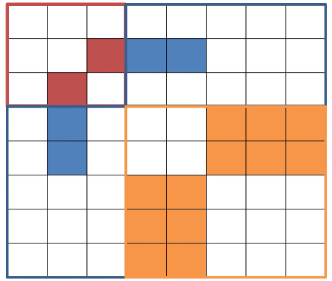
Figure 1: Symmetric matrix represents the parameters $\Theta$ of the model. This example has $p=3$, $q=2$, $L_{1}=2$ and $L_{2}=3$. The red square corresponds to the continuous graphical model coefficients $B$ and the solid red square is the scalar $\beta_{st}$. The blue square corresponds to the coefficients $\rho_{sj}$ and the solid blue square is a vector of parameters $\rho_{sj}(\cdot)$. The orange square corresponds to the coefficients $\phi_{rj}$ and the solid orange square is a matrix of parameters $\phi_{rj}(\cdot,\cdot)$. The matrix is symmetric, so each parameter block appears in two of the conditional probability regressions.

5 Calibrated regularizers

In (15) each of the group penalties are treated as equals, irrespective of the size of the group. We suggest a calibration or weighting scheme to balance the load in a more equitable way. We introduce weights for each group of parameters and show how to choose the weights such that each parameter set is treated equally under $p_{F}$, the fully-factorized independence model

$$\mathop{\rm minimize}_{\Theta}\ \ell(\Theta)+\lambda\left(\sum_{t=1}^{p}\sum_{t=1}^{s-1}w_{st}|\beta_{st}|+\sum_{s=1}^{p}\sum_{j=1}^{q}w_{sj}\left\|\rho_{sj}\right\|_{2}+\sum_{j=1}^{q}\sum_{r=1}^{j-1}w_{rj}\left\|\phi_{rj}\right\|_{F}\right)$$ (16)

Based on the KKT conditions (Friedman et al., 2007), the parameter group $\theta_{g}$ is non-zero if

$$\left\|\frac{\partial\ell}{\partial\theta_{g}}\right\|>\lambda w_{g}$$

where $\theta_{g}$ and $w_{g}$ represents one of the parameter groups and its corresponding weight. Now $\frac{\partial\ell}{\partial\theta_{g}}$ can be viewed as a generalized residual, and for different groups these are different dimensions—e.g. scalar/vector/matrix. So even under the independence model (when all terms should be zero), one might expect some terms $\left\|\frac{\partial\ell}{\partial\theta_{g}}\right\|$ to have a better random chance of being non-zero (for example, those of bigger dimensions). Thus for all parameters to be on equal footing, we would like to choose the weights $w$ such that

$$E_{p_{F}}\left\|\frac{\partial\ell}{\partial\theta_{g}}\right\|=\text{constant}\times w_{g}$$

However, it is simpler to compute in closed form $E_{p_{F}}\left\|\frac{\partial\ell}{\partial\theta_{g}}\right\|^{2}$, so we choose

$$w_{g}\propto\sqrt{E_{p_{F}}\left\|\frac{\partial\ell}{\partial\theta_{g}}\right\|^{2}}$$

where $p_{F}$ is the fully factorized (independence) model. In Appendix 9.6, we show that the weights can be chosen as

$$w_{st} =\sigma_{s}\sigma_{t}$$

$$w_{sj} =\sigma_{s}\sqrt{\sum_{a}p_{a}(1-p_{a})}$$

$$w_{rj} =\sqrt{\sum_{a}p_{a}(1-p_{a})\sum_{b}q_{b}(1-q_{b})}$$

$\sigma_{s}$ is the standard deviation of the continuous variable $x_{s}$. $p_{a}=Pr(y_{r}=a)$ and $q_{b}=Pr(y_{j}=b)$ . For all $3$ types of parameters, the weight has the form of $w_{uv}=\mathbf{tr}(\mathbf{cov}(z_{u}))\mathbf{tr}(\mathbf{cov}(z_{v}))$, where $z$ represents a generic variable and $\mathbf{cov}(z)$ is the variance-covariance matrix of $z$.

6 Model Selection Consistency

In this section, we study the model selection consistency, the correct edge set is selected and the parameter estimates are close to the truth, of pseudolikelihood and maximum likelihood. We will see that the consistency can be established using the framework first developed in Ravikumar et al. (2010) and later extended to general m-estimators by Lee et al. (2013). The proofs in this section are omitted since they follow from a straightforward application of the results in Lee et al. (2013); the results are stated for the mixed model to show that under certain conditions the estimation procedures are model selection consistent. We also only consider the uncalibrated regularizers to simplify the notation, but it is straightforward to adapt to the calibrated regularizer case.

First, we define some notation. Recall that $\Theta$ is the vector of parameters being estimated $\{\beta_{ss},\beta_{st},\alpha_{s},\phi_{rj},\rho_{sj}\}$, $\Theta^{\star}$ be the true parameters that estimated the model, and $Q=\nabla^{2}\ell(\Theta^{\star})$. Both estimation procedures can be written as a convex optimization problem of the form

$$\mathop{\rm minimize}\ \ell(\Theta)+\lambda\sum_{g\in G}\left\|\Theta_{g}\right\|_{2}$$ (17)

where $\ell(\theta)=\{\ell_{ML},\ell_{PL}\}$ is one of the two log-likelihoods. The regularizer

$$\sum_{g\in G}\left\|\Theta_{g}\right\|=\lambda\left(\sum_{s=1}^{p}\sum_{t=1}^{s-1}|\beta_{st}|+\sum_{s=1}^{p}\sum_{j=1}^{q}\left\|\rho_{sj}\right\|_{2}+\sum_{j=1}^{q}\sum_{r=1}^{j-1}\left\|\phi_{rj}\right\|_{F}\right).$$

The set $G$ indexes the edges $\beta_{st}$, $\rho_{sj}$, and $\phi_{rj}$, and $\Theta_{g}$ is one of the three types of edges.

It is difficult to establish consistency results for the problem in Equation (17) because the parameters are non-identifiable. This is because $\ell(\Theta)$ is constant with respect to the change of variables $\rho^{\prime}_{sj}(y_{j})=\rho_{sj}(y_{j})+c$ and similarly for $\phi$, so we cannot hope to recover $\Theta^{\star}$. A popular fix for this issue is to drop the last level of $\rho$ and $\phi$, so they are only indicators over $L-1$ levels instead of $L$ levels. This allows for the model to be identifiable, but it results in an asymmetric formulation that treats the last level differently from other levels. Instead, we will maintain the symmetric formulation by introducing constraints. Consider the problem

$$\mathop{\rm minimize}_{\Theta}\,\ \ell(\Theta)+\lambda\sum_{g\in G}\left\|\Theta_{g}\right\|_{2}$$ (18)

$$\text{subject to }C\Theta=0.$$

The matrix $C$ constrains the optimization variables such that

$$\sum_{y_{j}}\rho_{sj}(y_{j})=0$$

$$\sum_{y_{j}}\phi_{rj}(y_{r},y_{j})=0.$$

The group regularizer implicitly enforces the same set of constraints, so the optimization problems of Equation (18) and Equation (17) have the same solutions. For our theoretical results, we will use the constrained formulation of Equation (18), since it is identifiable.

We first state some definitions and two assumptions from Lee et al. (2013) that are necessary to present the model selection consistency results. Let $A$ and $I$ represent the active and inactive groups in $\Theta$, so $\Theta^{\star}_{g}\neq 0$ for any $g\in A$ and $\Theta_{g}^{\star}=0$ for any $g\in I$. The sets associated with the active and inactive groups are defined as

$$\mathcal{A} =\{\Theta\in\mathbb{R}^{d}:\max_{g\in G}\left\|\Theta_{g}\right\|_{2}\leq 1\;\textnormal{and }\left\|\Theta_{g}\right\|_{2}=0,\,g\in I\}$$

$$\mathcal{I} =\{\Theta\in\mathbb{R}^{d}:\max_{g\in G}\left\|\Theta_{g}\right\|_{2}\leq 1\;\textnormal{and }\left\|\Theta_{g}\right\|_{2}=0,\,g\in A\}.$$

Let $M=span(\mathcal{I})^{\perp}\cap Null(C)$ and $P_{M}$ be the orthogonal projector onto the subspace $M$. The two assumptions are

1. Restricted Strong Convexity. We assume that

   $$\sup_{v\in M}\frac{v^{T}\nabla^{2}\ell(\Theta)v}{v^{T}v}\geq m$$ (19)

   for all $\left\|\Theta-\Theta^{\star}\right\|_{2}\leq r$. Since $\nabla^{2}\ell(\Theta)$ is lipschitz continuous, the existence of a constant $m$ that satisfies (19) is implied by the pointwise restricted convexity

   $$\sup_{v\in M}\frac{v^{T}\nabla^{2}\ell(\Theta^{\star})v}{v^{T}v}\geq\tilde{m}.$$

   For convenience, we will use the former.

2. Irrepresentable condition. There exist $\tau\in(0,1)$ such that

   $$\sup_{z\in\mathcal{A}}\,V(P_{M^{\perp}}(\nabla^{2}\ell(\Theta^{\star})P_{M}(P_{M}\nabla^{2}\ell(\Theta^{\star})P_{M})^{\dagger}P_{M}z-z))<1-\tau,$$ (20)

   where $V$ is the infimal convolution of $\rho_{I}$, the gauge of set $\mathcal{I}$, and $\mathbbm{1}_{Null(C)^{\perp}}$:

   $$V(z)=\inf_{z=u_{1}+u_{2}}\,\{\rho_{I}(u_{1})+\mathbbm{1}_{Null(C)^{\perp}}(u_{2})\}.$$

Restricted strong convexity is a standard assumption that ensures the parameter $\Theta$ is uniquely determined by the value of the likelihood function. Without this, there is no hope of accurately estimating $\Theta^{\star}$. It is only stated over a subspace $M$ which can be much smaller than $\mathbb{R}^{d}$. The Irrepresentable condition is a more stringent condition. Intuitively, it requires that the active variables not be overly dependent on the inactive variables. Although the exact form of the condition is not enlightening, it is known to be ”almost” necessary for model selection consistency in the lasso (Zhao and Yu, 2006) and a common assumption in other works that establish model selection consistency (Ravikumar et al., 2010; Jalali et al., 2011; Peng et al., 2009). We also define the constants that appear in the theorem:

1. Lipschitz constants $L_{1}$ and $L_{2}$. Let $\Lambda(\Theta)$ be the log-partition function. $\Lambda(\Theta)$ and $\ell(\Theta)$ are twice continuously differentiable functions, so their gradient and hessian are locally Lipschitz continuous in a ball of radius $r$ around $\Theta^{\star}$:

   $$\left\|\nabla\Lambda(\Theta_{1})-\nabla\Lambda(\Theta_{2})\right\|_{2}\leq L_{1}\left\|\Theta_{1}-\Theta_{2}\right\|_{2},\ \Theta_{1},\Theta_{2}\in B_{r}(\Theta^{\star})$$

   $$\left\|\nabla^{2}\ell(\Theta_{1})-\nabla^{2}\ell(\Theta_{2})\right\|_{2}\leq L_{2}\left\|\Theta_{1}-\Theta_{2}\right\|_{2},\ \Theta_{1},\Theta_{2}\in B_{r}(\Theta^{\star})$$

2. Let $\bar{\tau}$ satisfy

   $$\sup_{z\in\mathcal{A}\cup\mathcal{I}}\,V(P_{M^{\perp}}(\nabla^{2}\ell(\Theta^{\star})P_{M}(P_{M}\nabla^{2}\ell(\Theta^{\star})P_{M})^{\dagger}P_{M}z-z))<\bar{\tau}.$$

   $V$ is a continuous function of $z$, so a finite $\bar{\tau}$ exists.

Theorem 2.

Suppose we are given samples $x^{(1)},\dots,x^{(n)}$ from the mixed model with unknown parameters $\Theta^{\star}$. If we select

$$\lambda=\frac{2\sqrt{256L_{1}}\bar{\tau}}{\tau}\sqrt{\frac{(\max_{g\in G}|g|)\log|G|}{n}}$$

and the sample size $n$ is larger than

$$\max\,\begin{cases}\frac{4096L_{1}L_{2}^{2}\bar{\tau}^{2}}{m^{4}\tau^{4}}\left(2+\frac{\tau}{\bar{\tau}}\right)^{4}(\max_{g\in G}|g|)|A|^{2}\log|G|\\ \frac{2048L_{1}}{m^{2}r^{2}}(2+\frac{\tau}{\bar{\tau}})^{2}(\max_{g\in G}|g|)|A|\log|G|,\end{cases}$$

then, with probability at least $1-2\big{(}\max_{g\in G}|g|\big{)}\exp(-c\lambda^{2}n)$, the optimal solution to (17) is unique and model selection consistent,

1. $\|\hat{\Theta}-\Theta^{\star}\|_{2}\leq\frac{4}{m}\left(\frac{\bar{\tau}+1}{2\tau}\right)\sqrt{\frac{256L_{1}|A|(\max_{g\in G}|g|)\log|G|}{n}},$

2. $\hat{\Theta}_{g}=0,\,g\in I$ and $\hat{\Theta}_{g}\neq 0\;\text{if }\left\|\Theta^{\star}_{g}\right\|_{2}>\frac{1}{m}\left(1+\frac{\tau}{2\bar{\tau}}\right)\sqrt{|A|}\lambda$.

Remark 3.

The same theorem applies to both the maximum likelihood and pseudolikelihood estimators. For the maximum likelihood, the constants can be tightened; everywhere $L_{1}$ appears can be replaced by $L_{1}/128$ and the theorem remains true. However, the values of $\tau,\bar{\tau},m,L_{1},L_{2}$ are different for the two methods. For the maximum likelihood, the gradient of the log-partition $\nabla\Lambda(\Theta)$ and hessian of the log-likelihood $\nabla^{2}\ell(\Theta)$ do not depend on the samples. Thus the constants $\tau,\bar{\tau},m,L_{1},L_{2}$ are completely determined by $\Theta^{\star}$ and the likelihood. For the pseudolikelihood, the values of $\tau,\bar{\tau},m,L_{2}$ depend on the samples, and the theorem only applies if the assumptions are made on sample quantities; thus, the theorem is less useful in practice when applied to the pseudolikelihood. This is similar to the situation in Yang et al. (2013), where assumptions are made on sample quantities.

7 Optimization Algorithms

In this section, we discuss two algorithms for solving (15): the proximal gradient and the proximal newton methods. This is a convex optimization problem that decomposes into the form $f(x)+g(x)$, where $f$ is smooth and convex and $g$ is convex but possibly non-smooth. In our case $f$ is the negative log-likelihood or negative log-pseudolikelihood and $g$ are the group sparsity penalties.

Block coordinate descent is a frequently used method when the non-smooth function $g$ is the $l_{1}$ or group $l_{1}$. It is especially easy to apply when the function $f$ is quadratic, since each block coordinate update can be solved in closed form for many different non-smooth $g$ (Friedman et al., 2007). The smooth $f$ in our particular case is not quadratic, so each block update cannot be solved in closed form. However in certain problems (sparse inverse covariance), the update can be approximately solved by using an appropriate inner optimization routine (Friedman et al., 2008b).

7.1 Proximal Gradient

Problems of this form are well-suited for the proximal gradient and accelerated proximal gradient algorithms as long as the proximal operator of $g$ can be computed (Combettes and Pesquet, 2011; Beck and Teboulle, 2010)

$$prox_{t}(x)=\mathop{\rm argmin}_{u}\frac{1}{2t}\left\|x-u\right\|^{2}+g(u)$$ (21)

For the sum of $l_{2}$ group sparsity penalties considered, the proximal operator takes the familiar form of soft-thresholding and group soft-thresholding (Bach et al., 2011). Since the groups are non-overlapping, the proximal operator simplifies to scalar soft-thresholding for $\beta_{st}$ and group soft-thresholding for $\rho_{sj}$ and $\phi_{rj}$.

The class of proximal gradient and accelerated proximal gradient algorithms is directly applicable to our problem. These algorithms work by solving a first-order model at the current iterate $x_{k}$

$$\mathop{\rm argmin}_{u}~{} f(x_{k})+\nabla f(x_{k})^{T}(u-x_{k})+\frac{1}{2t}\left\|u-x_{k}\right\|^{2}+g(u)$$ (22)

$$=\mathop{\rm argmin}_{u}~{}\frac{1}{2t}\left\|u-\left(x_{k}-t\nabla f(x_{k})\right)\right\|^{2}+g(u)$$ (23)

$$=prox_{t}(x_{k}-t\nabla f(x_{k}))$$ (24)

The proximal gradient iteration is given by $x_{k+1}=prox_{t}\left(x_{k}-t\nabla f(x_{k})\right)$ where $t$ is determined by line search. The theoretical convergence rates and properties of the proximal gradient algorithm and its accelerated variants are well-established (Beck and Teboulle, 2010). The accelerated proximal gradient method achieves linear convergence rate of $O(c^{k})$ when the objective is strongly convex and the sublinear rate $O(1/k^{2})$ for non-strongly convex problems.

The TFOCS framework (Becker et al., 2011) is a package that allows us to experiment with $6$ different variants of the accelerated proximal gradient algorithm. The TFOCS authors found that the Auslender-Teboulle algorithm exhibited less oscillatory behavior, and proximal gradient experiments in the next section were done using the Auslender-Teboulle implementation in TFOCS.

7.2 Proximal Newton Algorithms

This section borrows heavily from Schmidt (2010), Schmidt et al. (2011) and Lee et al. (2012). The class of proximal Newton algorithms is a 2nd order analog of the proximal gradient algorithms with a quadratic convergence rate (Lee et al., 2012). It attempts to incorporate 2nd order information about the smooth function $f$ into the model function. At each iteration, it minimizes a quadratic model centered at $x_{k}$

$$\mathop{\rm argmin}_{u}~{}f(x_{k})+\nabla f(x_{k})^{T}(u-x_{k})+\frac{1}{2t}(u-x_{k})^{T}H(u-x_{k})+g(u)$$ (25)

$$=\mathop{\rm argmin}_{u}~{}\frac{1}{2t}\left(u-x_{k}+tH^{-1}\nabla f(x_{k})\right)^{T}H\left(u-x_{k}+tH^{-1}\nabla f(x_{k})\right)+g(u)$$ (26)

$$=\mathop{\rm argmin}_{u}~{}\frac{1}{2t}\left\|u-\left(x_{k}-tH^{-1}\nabla f(x_{k})\right)\right\|^{2}_{H}+g(u)$$ (27)

$$:=Hprox_{t}\left(x_{k}-tH^{-1}\nabla f(x_{k})\right)\mbox{ where }H=\nabla^{2}f(x_{k})$$ (28)

Algorithm 1 Proximal Newton

repeat

     Solve subproblem $p_{k}=Hprox_{t}\left(x_{k}-tH_{k}^{-1}\nabla f(x_{k})\right)-x_{k}$ using TFOCS.

     Find $t$ to satisfy Armijo line search condition with parameter $\alpha$

$$f(x_{k}+tp_{k})+g(x_{k}+tp_{k})\leq f(x_{k})+g(x_{k})-\frac{t\alpha}{2}\left\|p_{k}\right\|^{2}$$

     Set $x_{k+1}=x_{k}+tp_{k}$

     $k=k+1$

until $\frac{\left\|x_{k}-x_{k+1}\right\|}{\left\|x_{k}\right\|}<tol$

The $Hprox$ operator is analogous to the proximal operator, but in the $\left\|\cdot\right\|_{H}$-norm. It simplifies to the proximal operator if $H=I$, but in the general case of positive definite $H$ there is no closed-form solution for many common non-smooth $g(x)$ (including $l_{1}$ and group $l_{1}$). However if the proximal operator of $g$ is available, each of these sub-problems can be solved efficiently with proximal gradient. In the case of separable $g$, coordinate descent is also applicable. Fast methods for solving the subproblem $Hprox_{t}(x_{k}-tH^{-1}\nabla f(x_{k}))$ include coordinate descent methods, proximal gradient methods, or Barzilai-Borwein (Friedman et al., 2007; Combettes and Pesquet, 2011; Beck and Teboulle, 2010; Wright et al., 2009). The proximal Newton framework allows us to bootstrap many previously developed solvers to the case of arbitrary loss function $f$.

Theoretical analysis in Lee et al. (2012) suggests that proximal Newton methods generally require fewer outer iterations (evaluations of $Hprox$) than first-order methods while providing higher accuracy because they incorporate 2nd order information. We have confirmed empirically that the proximal Newton methods are faster when $n$ is very large or the gradient is expensive to compute (e.g. maximum likelihood estimation). Since the objective is quadratic, coordinate descent is also applicable to the subproblems. The hessian matrix $H$ can be replaced by a quasi-newton approximation such as BFGS/L-BFGS/SR1. In our implementation, we use the PNOPT implementation (Lee et al., 2012).

7.3 Path Algorithm

Frequently in machine learning and statistics, the regularization parameter $\lambda$ is heavily dependent on the dataset. $\lambda$ is generally chosen via cross-validation or holdout set performance, so it is convenient to provide solutions over an interval of $[\lambda_{min},\lambda_{max}]$. We start the algorithm at $\lambda_{1}=\lambda_{max}$ and solve, using the previous solution as warm start, for $\lambda_{2}>\ldots>\lambda_{min}$. We find that this reduces the cost of fitting an entire path of solutions (See Figure 3). $\lambda_{max}$ can be chosen as the smallest value such that all parameters are $0$ by using the KKT equations (Friedman et al., 2007).

8 Conditional Model

We can generalize our mixed model, when there are additional features $f$, to a class of conditional random fields. Conditional models only model the conditional distribution $p(z|f)$, as opposed to the joint distribution $p(z,f)$, where $z$ are the variables of interest to the prediction task and $f$ are features.

In addition to observing $x$ and $y$, we observe features $f$ and we build a graphical model for the conditional distribution $p(x,y|f)$. Consider a full pairwise model $p(x,y,f)$ of the form (1). We then choose to only model the joint distribution over only the variables $x$ and $y$ to give us $p(x,y|f)$ which is of the form

$$p(x,y|f;\Theta)= \frac{1}{Z(\Theta|f)}\exp\left(\sum_{s=1}^{p}\sum_{t=1}^{p}-\frac{1}{2}\beta_{st}x_{s}x_{t}+\sum_{s=1}^{p}\alpha_{s}x_{s}+\sum_{s=1}^{p}\sum_{j=1}^{q}\rho_{sj}(y_{j})x_{s}\right.$$

$$\left.+\sum_{j=1}^{q}\sum_{r=1}^{j}\phi_{rj}(y_{r},y_{j})+\sum_{l=1}^{F}\sum_{s=1}^{p}\gamma_{ls}x_{s}f_{l}+\sum_{l=1}^{F}\sum_{r=1}^{q}\eta_{lr}(y_{r})f_{l}\right)$$ (29)

We can also consider a more general model where each pairwise edge potential depends on the features

$$p(x,y|f;\Theta)=\frac{1}{Z(\Theta|f)} \exp\left(\sum_{s=1}^{p}\sum_{t=1}^{p}-\frac{1}{2}\beta_{st}(f)x_{s}x_{t}+\sum_{s=1}^{p}\alpha_{s}(f)x_{s}\right.$$

$$\left.+\sum_{s=1}^{p}\sum_{j=1}^{q}\rho_{sj}(y_{j},f)x_{s}+\sum_{j=1}^{q}\sum_{r=1}^{j}\phi_{rj}(y_{r},y_{j},f)\vphantom{\sum_{s=1}^{p}\sum_{t=1}^{p}}\right)$$ (30)

(29) is a special case of this where only the node potentials depend on features and the pairwise potentials are independent of feature values. The specific parametrized form we consider is $\phi_{rj}(y_{r},y_{j},f)\equiv\phi_{rj}(y_{r},y_{j})$ for $r\neq j$, $\rho_{sj}(y_{j},f)\equiv\rho_{sj}(y_{j})$, and $\beta_{st}(f)=\beta_{st}$. The node potentials depend linearly on the feature values, $\alpha_{s}(f)=\alpha_{s}+\sum_{l=1}^{F}\gamma_{ls}x_{s}f_{l}$, and $\phi_{rr}(y_{r},y_{r},f)=\phi_{rr}(y_{r},y_{r})+\sum_{l}\eta_{lr}(y_{r})$.

9 Experimental Results

We present experimental results on synthetic data, survey data and on a conditional model.

9.1 Synthetic Experiments

In the synthetic experiment, the training points are sampled from a true model with $10$ continuous variables and $10$ binary variables. The edge structure is shown in Figure 2a. $\lambda$ is chosen as $5\sqrt{\frac{\log{p+q}}{n}}$ as suggested by the theoretical results in Section 6. We see from the experimental results that recovery of the correct edge set undergoes a sharp phase transition, as expected. With $n=1000$ samples, the pseudolikelihood is recovering the correct edge set with probability nearly $1$. The phase transition experiments were done using the proximal Newton algorithm discussed in Section 7.2.

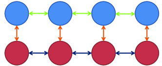
(a)

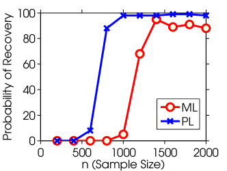
(b)

Figure 2: Figure 2a shows the graph used in the synthetic experiments for $p=q=4$; the experiment used $p$=10 and $q$=10. Blue nodes are continuous variables, red nodes are binary variables and the orange, green and dark blue lines represent the $3$ types of edges. Figure 2b is a plot of the probability of correct edge recovery at a given sample size using Maximum Likelihood and Pseudolikelihood. Results are averaged over $100$ trials.

9.2 Survey Experiments

The census survey dataset we consider consists of $11$ variables, of which $2$ are continuous and $9$ are discrete: age (continuous), log-wage (continuous), year($7$ states), sex($2$ states),marital status ($5$ states), race($4$ states), education level ($5$ states), geographic region($9$ states), job class ($2$ states), health ($2$ states), and health insurance ($2$ states). The dataset was assembled by Steve Miller of OpenBI.com from the March 2011 Supplement to Current Population Survey data. All the evaluations are done using a holdout test set of size $100,000$ for the survey experiments. The regularization parameter $\lambda$ is varied over the interval $[5\times 10^{-5},0.7]$ at $50$ points equispaced on log-scale for all experiments.

9.2.1 Model Selection

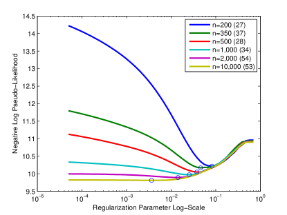
Figure 3: Model selection under different training set sizes. Circle denotes the lowest test set negative log pseudolikelihood and the number in parentheses is the number of edges in that model at the lowest test negative log pseudolikelihood. The saturated model has $55$ edges.

In Figure 3, we study the model selection performance of learning a graphical model over the $11$ variables under different training samples sizes. We see that as the sample size increases, the optimal model is increasingly dense, and less regularization is needed.

9.2.2 Comparing against Separate Regressions

A sensible baseline method to compare against is a separate regression algorithm. This algorithm fits a linear Gaussian or (multiclass) logistic regression of each variable conditioned on the rest. We can evaluate the performance of the pseudolikelihood by evaluating $-\log{p(x_{s}|x_{\backslash s},y)}$ for linear regression and $-\log{p(y_{r}|y_{\backslash r},x)}$ for (multiclass) logistic regression. Since regression is directly optimizing this loss function, it is expected to do better. The pseudolikelihood objective is similar, but has half the number of parameters as the separate regressions since the coefficients are shared between two of the conditional likelihoods. From Figures 4 and 5, we can see that the pseudolikelihood performs very similarly to the separate regressions and sometimes even outperforms regression. The benefit of the pseudolikelihood is that we have learned parameters of the joint distribution $p(x,y)$ and not just of the conditionals $p(x_{s}|y,x_{\backslash s})$. On the test dataset, we can compute quantities such as conditionals over arbitrary sets of variables $p(y_{A},x_{B}|y_{A^{C}},x_{B^{C}})$ and marginals $p(x_{A},y_{B})$ (Koller and Friedman, 2009). This would not be possible using the separate regressions.

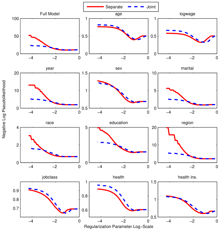
Figure 4: Separate Regression vs Pseudolikelihood $n=100$. $y$-axis is the appropriate regression loss for the response variable. For low levels of regularization and at small training sizes, the pseudolikelihood seems to overfit less; this may be due to a global regularization effect from fitting the joint distribution as opposed to separate regressions.

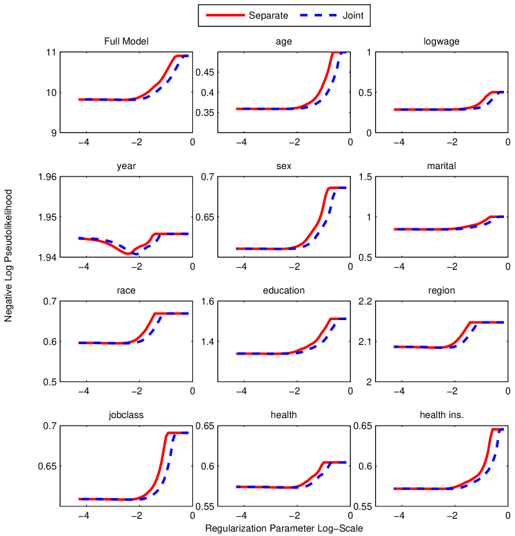
Figure 5: Separate Regression vs Pseudolikelihood $n=10,000$. $y$-axis is the appropriate regression loss for the response variable. At large sample sizes, separate regressions and pseudolikelihood perform very similarly. This is expected since this is nearing the asymptotic regime.

9.2.3 Conditional Model

Using the conditional model (29), we model only the $3$ variables logwage, education($5$) and jobclass($2$). The other $8$ variables are only used as features. The conditional model is then trained using the pseudolikelihood. We compare against the generative model that learns a joint distribution on all $11$ variables. From Figure 6, we see that the conditional model outperforms the generative model, except at small sample sizes. This is expected since the conditional distribution models less variables. At very small sample sizes and small $\lambda$, the generative model outperforms the conditional model. This is likely because generative models converge faster (with less samples) than discriminative models to its optimum.

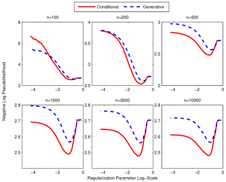
Figure 6: Conditional Model vs Generative Model at various sample sizes. $y$-axis is test set performance is evaluated on negative log pseudolikelihood of the conditional model. The conditional model outperforms the full generative model at except the smallest sample size $n=100$.

9.2.4 Maximum Likelihood vs Pseudolikelihood

The maximum likelihood estimates are computable for very small models such as the conditional model previously studied. The pseudolikelihood was originally motivated as an approximation to the likelihood that is computationally tractable. We compare the maximum likelihood and maximum pseudolikelihood on two different evaluation criteria: the negative log likelihood and negative log pseudolikelihood. In Figure 7, we find that the pseudolikelihood outperforms maximum likelihood under both the negative log likelihood and negative log pseudolikelihood. We would expect that the pseudolikelihood trained model does better on the pseudolikelihood evaluation and maximum likelihood trained model does better on the likelihood evaluation. However, we found that the pseudolikelihood trained model outperformed the maximum likelihood trained model on both evaluation criteria. Although asymptotic theory suggests that maximum likelihood is more efficient than the pseudolikelihood, this analysis is applicable because of the finite sample regime and misspecified model. See Liang and Jordan (2008) for asymptotic analysis of pseudolikelihood and maximum likelihood under a well-specified model. We also observed the pseudolikelihood slightly outperforming the maximum likelihood in the synthetic experiment of Figure 2b.

Figure 7: Maximum Likelihood vs Pseudolikelihood. $y$-axis for top row is the negative log pseudolikelihood. $y$-axis for bottom row is the negative log likelihood. Pseudolikelihood outperforms maximum likelihood across all the experiments.

Appendix

9.3 Proof of Convexity

Proposition 1.The negative log pseudolikelihood in (9) is jointly convex in all the parameters $\{\beta_{ss},\beta_{st},\alpha_{s},\phi_{rj},\rho_{sj}\}$ over the region $\beta_{ss}>0$.

Proof.

To verify the convexity of $\tilde{\ell}(\Theta|x,y)$, it suffices to check that each term is convex. $-\log{p(y_{r}|y_{\backslash r,},x;\Theta)}$ is jointly convex in $\rho$ and $\phi$ since it is a multiclass logistic regression. We now check that $-\log{p(x_{s}|x_{\backslash s},y;\Theta)}$ is convex. $-\frac{1}{2}\log{\beta_{ss}}$ is a convex function. To establish that $\frac{\beta_{ss}}{2}\left(\frac{\alpha_{s}}{\beta_{ss}}+\sum_{j}\frac{\rho_{sj}(y_{j})}{\beta_{ss}}-\sum_{t\neq s}\frac{\beta_{st}}{\beta_{ss}}x_{t}-x_{s}\right)^{2}$ is convex, we use the fact that $f(u,v)=\frac{v}{2}(\frac{u}{v}-c)^{2}$ is convex. Let $v=\beta_{ss}$, $u=\alpha_{s}+\sum_{j}\rho_{sj}(y_{j})-\sum_{t\neq s}\beta_{st}x_{t}$, and $c=x_{s}$. Notice that $x_{s}$, $\alpha_{s}$, $y_{j}$, and $x_{t}$ are fixed quantities and $u$ is affinely related to $\beta_{st}$ and $\rho_{sj}$. A convex function composed with an affine map is still convex, thus $\frac{\beta_{ss}}{2}\left(\frac{\alpha_{s}}{\beta_{ss}}+\sum_{j}\frac{\rho_{sj}(y_{j})}{\beta_{ss}}-\sum_{t\neq s}\frac{\beta_{st}}{\beta_{ss}}x_{t}-x_{s}\right)^{2}$ is convex.

To finish the proof, we verify that $f(u,v)=\frac{v}{2}(\frac{u}{v}-c)^{2}=\frac{1}{2}\frac{(u-cv)^{2}}{v}$ is convex over $v>0$. The epigraph of a convex function is a convex set iff the function is convex. Thus we establish that the set $C=\{(u,v,t)|\frac{1}{2}\frac{(u-cv)^{2}}{v}\leq t,v>0\}$ is convex. Let $A=\begin{bmatrix}v&u-cv\\ u-cv&t\end{bmatrix}.$ The Schur complement criterion of positive definiteness says $A\succ 0$ iff $v>0$ and $t>\frac{(u-cv)^{2}}{v}$. The condition $A\succ 0$ is a linear matrix inequality and thus convex in the entries of $A$. The entries of $A$ are linearly related to $u$ and $v$, so $A\succ 0$ is also convex in $u$ and $v$. Therefore $v>0$ and $t>\frac{(u-cv)^{2}}{v}$ is a convex set. ∎

9.4 Sampling From The Joint Distribution

In this section we discuss how to draw samples $(x,y)\thicksim p(x,y)$. Using the property that $p(x,y)=p(y)p(x|y)$, we see that if $y\thicksim p(y)$ and $x\thicksim p(x|y)$ then $(x,y)\thicksim p(x,y)$. We have that

$$p(y) \propto\exp{(\sum_{r,j}\phi_{rj}(y_{r},y_{j})+\frac{1}{2}\rho(y)^{T}B^{-1}\rho(y))}$$ (31)

$$(\rho(y))_{s} =\sum_{j}\rho_{sj}(y_{j})$$ (32)

$$p(x|y) =No(B^{-1}(\alpha+\rho(y)),B^{-1})$$ (33)

The difficult part is to sample $y\thicksim p(y)$ since this involves the partition function of the discrete MRF. This can be done with MCMC for larger models and junction tree algorithm or exact sampling for small models.

9.5 Maximum Likelihood

The difficulty in MLE is that in each gradient step we have to compute $\hat{T}(x,y)-E_{p(\Theta)}\left[T(x,y)\right]$, the difference between the empirical sufficient statistic $\hat{T}(x,y)$ and the expected sufficient statistic. In both continuous and discrete graphical models the computationally expensive step is evaluating $E_{p(\Theta)}\left[T(x,y)\right]$. In discrete problems, this involves a sum over the discrete state space and in continuous problem, this requires matrix inversion. For both discrete and continuous models, there has been much work on addressing these difficulties. For discrete models, the junction tree algorithm is an exact method for evaluating marginals and is suitable for models with low tree width. Variational methods such as belief propagation and tree reweighted belief propagation work by optimizing a surrogate likelihood function by approximating the partition function $Z(\Theta)$ by a tractable surrogate $\widetilde{Z}(\Theta)$ Wainwright and Jordan (2008). In the case of a large discrete state space, these methods can be used to approximate $p(y)$ and do approximate maximum likelihood estimation for the discrete model. Approximate maximum likelihood estimation can also be done via Monte Carlo estimates of the gradients $\hat{T}(x,y)-E_{p(\Theta)}(T(x,y))$. For continuous Gaussian graphical models, efficient algorithms based on block coordinate descent Friedman et al. (2008b); Banerjee et al. (2008) have been developed, that do not require matrix inversion.

The joint distribution and loglikelihood are:

$$p(x,y;\Theta) =\exp{(-\frac{1}{2}x^{T}Bx+(\alpha+\rho(y))^{T}x+\sum_{(r,j)}\phi_{rj}(y_{r},y_{j}))}/Z(\Theta)$$

$$\ell(\Theta) =\left(\frac{1}{2}x^{T}Bx-(\alpha+\rho(y))^{T}x-\sum_{(r,j)}\phi_{rj}(y_{r},y_{j})\right)$$

$$+\log(\sum_{y^{\prime}}\int{dx\exp{(-\frac{1}{2}x^{T}Bx+(\alpha+\rho(y^{\prime}))^{T}x)}}\exp(\sum_{(r,j)}\phi_{rj}(y^{\prime}_{r},y^{\prime}_{j})))$$

The derivative is

$$\frac{\partial\ell}{\partial B} =\frac{1}{2}xx^{T}+\frac{\int dx(\sum_{y^{\prime}}-\frac{1}{2}xx^{T}\exp(-\frac{1}{2}x^{T}Bx+(\alpha+\rho(y))^{T}x+\sum_{(r,j)}\phi_{rj}(y^{\prime}_{r},y^{\prime}_{j})))}{Z(\Theta)}$$

$$=\frac{1}{2}xx^{T}+\int\sum_{y^{\prime}}(-\frac{1}{2}xx^{T}p(x,y^{\prime};\Theta))$$

$$=\frac{1}{2}xx^{T}+\sum_{y^{\prime}}\int-\frac{1}{2}xx^{T}p(x|y^{\prime};\Theta)p(y^{\prime})$$

$$=\frac{1}{2}xx^{T}+\sum_{y^{\prime}}\int-\frac{1}{2}\left(B^{-1}+B^{-1}(\alpha+\rho(y^{\prime}))(\alpha+\rho(y^{\prime})^{T})B^{-1}\right)p(y^{\prime})$$

The primary cost is to compute $B^{-1}$ and the sum over the discrete states $y$.
The computation for the derivatives of $\ell(\Theta)$ with respect to $\rho_{sj}$ and $\phi_{rj}$ are similar.

$$\frac{\partial\ell}{\phi_{rj}(a,b)} =-1(y_{r}=a,y_{j}=b)+\sum_{y^{\prime}}\int dx1(y^{\prime}_{r}=a,y^{\prime}_{j}=b)p(x,y^{\prime};\Theta)$$

$$=-1(y_{r}=a,y_{j}=b)+\sum_{y^{\prime}}1(y^{\prime}_{r}=a,y^{\prime}_{j}=b)p(y^{\prime})$$

The gradient requires summing over all discrete states.
Similarly for $\rho_{sj}(a)$:

$$\frac{\partial\ell}{\rho_{sj}(a)}=-1(y_{j}=a)x_{s}+\sum_{y^{\prime}}\int dx(1(y^{\prime}_{j}=a)x_{s})p(x^{\prime},y^{\prime};\Theta)$$

$$=-1(y_{j}=a)x_{s}+\int dx\sum_{y_{\backslash j}^{\prime}}x_{s}p(x|y^{\prime}_{\backslash j},y^{\prime}_{j}=a)p(y^{\prime}_{\backslash j},y^{\prime}_{j}=a)$$

MLE estimation requires summing over the discrete states to compute the expected sufficient statistics. This may be approximated using using samples $(x,y)\thicksim p(x,y;\Theta)$. The method in the previous section shows that sampling is efficient if $y\thicksim p(y)$ is efficient. This allows us to use MCMC methods developed for discrete MRF’s such as Gibbs sampling.

9.6 Choosing the Weights

We first show how to compute $w_{sj}$. The gradient of the pseudo-likelihood with respect to a parameter $\rho_{sj}(a)$ is given below

$$\frac{\partial\tilde{\ell}}{\partial\rho_{sj}(a)} =\sum_{i=1}^{n}-2\times\mathbbm{1}{\left[{y_{j}^{i}=a}\right]}x_{s}^{i}+E_{p_{F}}(\mathbbm{1}{\left[{y_{j}=a}\right]}x_{s}|y_{\backslash j}^{i},x^{i})+E_{p_{F}}(\mathbbm{1}{\left[{y_{j}=a}\right]}x_{s}|x^{i}_{\backslash s},y^{i})$$

$$=\sum_{i=1}^{n}-2\times\mathbbm{1}{\left[{y_{j}^{i}=a}\right]}x_{s}^{i}+x^{i}_{s}p(y_{j}=a)+\mathbbm{1}{\left[{y_{j}^{i}=a}\right]}\mu_{s}$$

$$=\sum_{i=1}^{n}\mathbbm{1}{\left[{y_{j}^{i}=a}\right]}\left(\hat{\mu}_{s}-x^{i}_{s}\right)+x_{s}^{i}\left(\hat{p}(y_{j}=a)-\mathbbm{1}{\left[{y_{j}^{i}=a}\right]}\right)$$

$$=\sum_{i=1}^{n}\left(\mathbbm{1}{\left[{y_{j}^{i}=a}\right]}-\hat{p}(y_{j}=a)\right)\left(\hat{\mu}_{s}-x^{i}_{s}\right)+\left(x_{s}^{i}-\hat{\mu}_{s}\right)\left(\hat{p}(y_{j}=a)-\mathbbm{1}{\left[{y_{j}^{i}=a}\right]}\right)$$ (34)

$$=\sum_{i=1}^{n}2\left(\mathbbm{1}{\left[{y_{j}^{i}=a}\right]}-\hat{p}(y_{j}=a)\right)\left(\hat{\mu}_{s}-x^{i}_{s}\right)$$ (35)

Since the subgradient condition includes a variable if $\left\|\frac{\partial\tilde{\ell}}{\partial\rho_{sj}}\right\|>\lambda$, we compute $E\left\|\frac{\partial\tilde{\ell}}{\partial\rho_{sj}}\right\|^{2}$. By independence,

$$E_{p_{F}}\left(\left\|\sum_{i=1}^{n}2\left(\mathbbm{1}{\left[{y_{j}^{i}=a}\right]}-\hat{p}(y_{j}=a)\right)\left(\hat{\mu}_{s}-x^{i}_{s}\right)\right\|^{2}\right)$$ (36)

$$=4nE_{p_{F}}\left(\left\|\mathbbm{1}{\left[{y_{j}^{i}=a}\right]}-\hat{p}(y_{j}=a)\right\|^{2}\right)E_{p_{F}}\left(\left\|\hat{\mu}_{s}-x^{i}_{s}\right\|^{2}\right)$$ (37)

$$=4(n-1)p(y_{j}=a)(1-p(y_{j}=a))\sigma_{s}^{2}$$ (38)

The last line is an equality if we replace the sample means $\hat{p}$ and $\hat{\mu}$ with the true values $p$ and $\mu$. Thus for the entire vector $\rho_{sj}$ we have $E_{p_{F}}\left\|\frac{\partial\tilde{\ell}}{\partial\rho_{sj}}\right\|^{2}=4(n-1)\left(\sum_{a}p(y_{j}=a)(1-p(y_{j}=a)\right)\sigma_{s}^{2}$. If we let the vector $z$ be the indicator vector of the categorical variable $y_{j}$, and let the vector $p=p(y_{j}=a)$, then $E_{p_{F}}\left\|\frac{\partial\tilde{\ell}}{\partial\rho_{sj}}\right\|^{2}=4(n-1)\sum_{a}p_{a}(1-p_{a})\sigma^{2}=4(n-1)\mathbf{tr}(\mathbf{cov}(z))\mathbf{var}(x)$ and $w_{sj}=\sqrt{\sum_{a}p_{a}(1-p_{a})\sigma_{s}^{2}}$.

We repeat the computation for $\beta_{st}$.

$$\frac{\partial\ell}{\partial\beta_{st}} =\sum_{i=1}^{n}-2x^{i}_{s}x_{t}+E_{p_{F}}(x^{i}_{s}x^{i}_{t}|x_{\backslash s},y)+E_{p_{F}}(x^{i}_{s}x^{i}_{t}|x_{\backslash t},y)$$

$$=\sum_{i=1}^{n}-2x^{i}_{s}x^{i}_{t}+\hat{\mu}_{s}x^{i}_{t}+\hat{\mu}_{t}x^{i}_{s}$$

$$=\sum_{i=1}^{n}x^{i}_{t}(\hat{\mu_{s}}-x^{i}_{s})+x^{i}_{s}(\hat{\mu}_{t}-x^{i}_{t})$$

$$=\sum_{i=1}^{n}(x^{i}_{t}-\hat{\mu}_{t})(\hat{\mu_{s}}-x^{i}_{s})+(x^{i}_{s}-\hat{\mu_{s}})(\hat{\mu_{t}}-x^{i}_{t})$$

$$=\sum_{i=1}^{n}2(x^{i}_{t}-\hat{\mu}_{t})(\hat{\mu_{s}}-x^{i}_{s})$$

Thus

$$E \left(\left\|\sum_{i=1}^{n}2(x^{i}_{t}-\hat{\mu}_{t})(\hat{\mu_{s}}-x^{i}_{s})\right\|^{2}\right)$$

$$=4nE_{p_{F}}\left\|x_{t}-\hat{\mu_{t}}\right\|^{2}E_{p_{F}}\left\|x_{s}-\hat{\mu}_{s}\right\|^{2}$$

$$=4(n-1)\sigma_{s}^{2}\sigma_{t}^{2}$$

Thus $E_{p_{F}}\left\|\frac{\partial\ell}{\partial\beta_{st}}\right\|^{2}=4(n-1)\sigma_{s}^{2}\sigma_{t}^{2}$ and taking square-roots gives us $w_{st}=\sigma_{s}\sigma_{t}$.
We repeat the same computation for $\phi_{rj}$. Let $p_{a}=Pr(y_{r}=a)$ and $q_{b}=Pr(y_{j}=b)$.

$$\frac{\partial\tilde{\ell}}{\partial\phi_{rj}(a,b)} =\sum_{i=1}^{n}-\mathbbm{1}{\left[{y^{i}_{r}=a}\right]}\mathbbm{1}{\left[{y^{i}_{j}=b}\right]}+E\left(\mathbbm{1}{\left[{y_{r}=a}\right]}\mathbbm{1}{\left[{y_{j}=b}\right]}|y_{\backslash r},x\right)$$

$$+E\left(\mathbbm{1}{\left[{y_{r}=a}\right]}\mathbbm{1}{\left[{y_{j}=b}\right]}|y_{\backslash j},x\right)$$

$$=\sum_{i=1}^{n}-\mathbbm{1}{\left[{y^{i}_{r}=a}\right]}\mathbbm{1}{\left[{y^{i}_{j}=b}\right]}+\hat{p}_{a}\mathbbm{1}{\left[{y^{i}_{j}=b}\right]}+\hat{q}_{b}\mathbbm{1}{\left[{y^{i}_{r}=a}\right]}$$

$$=\sum_{i=1}^{n}\mathbbm{1}{\left[{y^{i}_{j}=b}\right]}(\hat{p}_{a}-\mathbbm{1}{\left[{y^{i}_{r}=a}\right]})+\mathbbm{1}{\left[{y^{i}_{r}=a}\right]}(\hat{q}_{b}-\mathbbm{1}{\left[{y^{i}_{j}=b}\right]})$$

$$=\sum_{i=1}^{n}(\mathbbm{1}{\left[{y^{i}_{j}=b}\right]}-\hat{q}_{b})(\hat{p}_{a}-\mathbbm{1}{\left[{y^{i}_{r}=a}\right]})+(\mathbbm{1}{\left[{y^{i}_{r}=a}\right]}-\hat{p}_{a})(\hat{q}_{b}-\mathbbm{1}{\left[{y^{i}_{j}=b}\right]})$$

$$=\sum_{i=1}^{n}2(\mathbbm{1}{\left[{y^{i}_{j}=b}\right]}-\hat{q}_{b})(\hat{p}_{a}-\mathbbm{1}{\left[{y^{i}_{r}=a}\right]})$$

Thus we compute

$$E_{p_{F}}\left\|\frac{\partial\tilde{\ell}}{\partial\phi_{rj}(a,b)}\right\|^{2} =E\left(\left\|\sum_{i=1}^{n}2(\mathbbm{1}{\left[{y^{i}_{j}=b}\right]}-\hat{q}_{b})(\hat{p}_{a}-\mathbbm{1}{\left[{y^{i}_{r}=a}\right]})\right\|^{2}\right)$$

$$=4nE_{p_{F}}\left\|\hat{q}_{b}-\mathbbm{1}{\left[{y_{j}=b}\right]}\right\|^{2}E_{p_{F}}\left\|\hat{p}_{a}-\mathbbm{1}{\left[{y_{r}=a}\right]}\right\|^{2}$$

$$=4(n-1)q_{b}(1-q_{b})p_{a}(1-p_{a})$$

From this, we see that $E_{p_{F}}\left\|\frac{\partial\tilde{\ell}}{\partial\phi_{rj}}\right\|^{2}=\sum_{a=1}^{L_{r}}\sum_{b=1}^{L_{j}}4(n-1)q_{b}(1-q_{b})p_{a}(1-p_{a})$ and $w_{rj}=\sqrt{\sum_{a=1}^{L_{r}}\sum_{b=1}^{L_{j}}q_{b}(1-q_{b})p_{a}(1-p_{a})}$.

References

• Bach et al. (2011) F. Bach, R. Jenatton, J. Mairal, and G. Obozinski. Optimization with sparsity-inducing penalties. Foundations and Trends in Machine Learning, 4:1–106, 2011. URL http://dx.doi.org/10.1561/2200000015.
• Banerjee et al. (2008) O. Banerjee, L. El Ghaoui, and A. d’Aspremont. Model selection through sparse maximum likelihood estimation for multivariate gaussian or binary data. The Journal of Machine Learning Research, 9:485–516, 2008.
• Beck and Teboulle (2010) A. Beck and M. Teboulle. Gradient-based algorithms with applications to signal recovery problems. Convex Optimization in Signal Processing and Communications, pages 42–88, 2010.
• Becker et al. (2011) S.R. Becker, E.J. Candès, and M.C. Grant. Templates for convex cone problems with applications to sparse signal recovery. Mathematical Programming Computation, pages 1–54, 2011.
• Besag (1974) J. Besag. Spatial interaction and the statistical analysis of lattice systems. Journal of the Royal Statistical Society. Series B (Methodological), pages 192–236, 1974.
• Besag (1975) J. Besag. Statistical analysis of non-lattice data. The statistician, pages 179–195, 1975.
• Combettes and Pesquet (2011) P.L. Combettes and J.C. Pesquet. Proximal splitting methods in signal processing. Fixed-Point Algorithms for Inverse Problems in Science and Engineering, pages 185–212, 2011.
• Edwards (2000) D. Edwards. Introduction to graphical modelling. Springer, 2000.
• Friedman et al. (2007) J. Friedman, T. Hastie, H. Höfling, and R. Tibshirani. Pathwise coordinate optimization. The Annals of Applied Statistics, 1(2):302–332, 2007.
• Friedman et al. (2008a) J. Friedman, T. Hastie, and R. Tibshirani. Sparse inverse covariance estimation with the graphical lasso. Biostatistics, 9(3):432–441, 2008a.
• Friedman et al. (2008b) J. Friedman, T. Hastie, and R. Tibshirani. Sparse inverse covariance estimation with the graphical lasso. Biostatistics, 9(3):432–441, 2008b.
• Friedman et al. (2010) J. Friedman, T. Hastie, and R. Tibshirani. Applications of the lasso and grouped lasso to the estimation of sparse graphical models. Technical report, Technical Report, Stanford University, 2010.
• Guo et al. (2010) J. Guo, E. Levina, G. Michailidis, and J. Zhu. Joint structure estimation for categorical markov networks. Submitted. Available at http://www. stat. lsa. umich. edu/~ elevina, 2010.
• Höfling and Tibshirani (2009) H. Höfling and R. Tibshirani. Estimation of sparse binary pairwise markov networks using pseudo-likelihoods. The Journal of Machine Learning Research, 10:883–906, 2009.
• Jalali et al. (2011) A. Jalali, P. Ravikumar, V. Vasuki, S. Sanghavi, UT ECE, and UT CS. On learning discrete graphical models using group-sparse regularization. In Proceedings of the International Conference on Artificial Intelligence and Statistics (AISTATS), 2011.
• Kim et al. (2009) Seyoung Kim, Kyung-Ah Sohn, and Eric P Xing. A multivariate regression approach to association analysis of a quantitative trait network. Bioinformatics, 25(12):i204–i212, 2009.
• Koller and Friedman (2009) D. Koller and N. Friedman. Probabilistic graphical models: principles and techniques. The MIT Press, 2009.
• Lauritzen (1996) S.L. Lauritzen. Graphical models, volume 17. Oxford University Press, USA, 1996.
• Lee et al. (2013) Jason D Lee, Yuekai Sun, and Jonathan Taylor. On model selection consistency of m-estimators with geometrically decomposable penalties. arXiv preprint arXiv:1305.7477, 2013.
• Lee et al. (2012) J.D. Lee, Y. Sun, and M.A. Saunders. Proximal newton-type methods for minimizing convex objective functions in composite form. arXiv preprint arXiv:1206.1623, 2012.
• Lee et al. (2006) S.I. Lee, V. Ganapathi, and D. Koller. Efficient structure learning of markov networks using l1regularization. In NIPS, 2006.
• Liang and Jordan (2008) P. Liang and M.I. Jordan. An asymptotic analysis of generative, discriminative, and pseudolikelihood estimators. In Proceedings of the 25th international conference on Machine learning, pages 584–591. ACM, 2008.
• Liu and Ihler (2011) Q. Liu and A. Ihler. Learning scale free networks by reweighted l1 regularization. In Proceedings of the 14th International Conference on Artificial Intelligence and Statistics (AISTATS), 2011.
• Liu and Ihler (2012) Q. Liu and A. Ihler. Distributed parameter estimation via pseudo-likelihood. In Proceedings of the International Conference on Machine Learning (ICML), 2012.
• Meinshausen and Bühlmann (2006) N. Meinshausen and P. Bühlmann. High-dimensional graphs and variable selection with the lasso. The Annals of Statistics, 34(3):1436–1462, 2006.
• Peng et al. (2009) J. Peng, P. Wang, N. Zhou, and J. Zhu. Partial correlation estimation by joint sparse regression models. Journal of the American Statistical Association, 104(486):735–746, 2009.
• Ravikumar et al. (2010) P. Ravikumar, M.J. Wainwright, and J.D. Lafferty. High-dimensional ising model selection using l1-regularized logistic regression. The Annals of Statistics, 38(3):1287–1319, 2010.
• Rothman et al. (2010) Adam J Rothman, Elizaveta Levina, and Ji Zhu. Sparse multivariate regression with covariance estimation. Journal of Computational and Graphical Statistics, 19(4):947–962, 2010.
• Schmidt (2010) M. Schmidt. Graphical Model Structure Learning with l1-Regularization. PhD thesis, University of British Columbia, 2010.
• Schmidt et al. (2008) M. Schmidt, K. Murphy, G. Fung, and R. Rosales. Structure learning in random fields for heart motion abnormality detection. CVPR. IEEE Computer Society, 2008.
• Schmidt et al. (2011) M. Schmidt, D. Kim, and S. Sra. Projected newton-type methods in machine learning. 2011.
• Tur and Castelo (2012) Inma Tur and Robert Castelo. Learning mixed graphical models from data with p larger than n. arXiv preprint arXiv:1202.3765, 2012.
• Wainwright and Jordan (2008) M.J. Wainwright and M.I. Jordan. Graphical models, exponential families, and variational inference. Foundations and Trends® in Machine Learning, 1(1-2):1–305, 2008.
• Witten and Tibshirani (2009) Daniela M Witten and Robert Tibshirani. Covariance-regularized regression and classification for high dimensional problems. Journal of the Royal Statistical Society: Series B (Statistical Methodology), 71(3):615–636, 2009.
• Wright et al. (2009) S.J. Wright, R.D. Nowak, and M.A.T. Figueiredo. Sparse reconstruction by separable approximation. Signal Processing, IEEE Transactions on, 57(7):2479–2493, 2009.
• Yang et al. (2012) E. Yang, P. Ravikumar, G. Allen, and Z. Liu. Graphical models via generalized linear models. In Advances in Neural Information Processing Systems 25, pages 1367–1375, 2012.
• Yang et al. (2013) E. Yang, P. Ravikumar, G.I. Allen, and Z. Liu. On graphical models via univariate exponential family distributions. arXiv preprint arXiv:1301.4183, 2013.
• Yuan and Lin (2006) M. Yuan and Y. Lin. Model selection and estimation in regression with grouped variables. Journal of the Royal Statistical Society: Series B (Statistical Methodology), 68(1):49–67, 2006.
• Zhao and Yu (2006) Peng Zhao and Bin Yu. On model selection consistency of lasso. The Journal of Machine Learning Research, 7:2541–2563, 2006.