Spin-chain description of fractional quantum Hall states in the Jain series

Abstract

We discuss the relationship between fractional quantum Hall (FQH) states at filling factor $\nu=p/(2p+1)$ and quantum spin chains. This series corresponds to the Jain series $\nu=p/(2mp+1)$ with $m=1$ where the composite fermion picture is realized. We show that the FQH states with toroidal boundary conditions beyond the thin-torus limit can be mapped to effective quantum spin $S=1$ chains with $p$ spins in each unit cell. We calculate energy gaps and the correlation functions for both the FQH systems and the corresponding effective spin chains, using exact diagonalization and the infinite time-evolving block decimation (iTEBD) algorithm. We confirm that the mass gaps of these effective spin chains are decreased as $p$ is increased which is similar to $S=p$ integer Heisenberg chains. These results shed new light on a link between the hierarchy of FQH states and the Haldane conjecture for quantum spin chains.

I Introduction

The fractional quantum Hall (FQH) state,QH interacting cold electrons in two-dimensional space in a strong perpendicular magnetic field, exhibits fascinating phases with fractionalized excitations and topological order.Laughlin ; Haldane ; Halperin ; Jain ; Moore-R Ever since its discovery three decades ago, the FQH system has inspired a huge amount of experimental and theoretical effort, due to its richness in phenomenology and mathematical structure. New developments include the observation of the FQH in graphene fqhgraphene , topological quantum computing qcomp , and systems of rapidly rotating bosons which are formally very similar to those of an electron gas in a magnetic field.boseQH

On the other hand, it has been pointed out that the hierarchy of FQH states has striking similarities to the quantum spin chains.Girvin-A Haldane conjectured Haldane1983 that half-integer SU(2) Heisenberg chains support gapless excitations, protected by a topological term in the effective action, while the integer spin chains develop a mass gap. A similar structure appears in the FQH effect. At filling factors $\nu<1$, quantized conductance plateaus only occur at rational $\nu$ with odd denominator, while in the vicinity of even-denominator fractions metallic behavior is sustained. Hence, it is important to establish whether the similarities are merely accidental or whether the structure of low-energy excitations in these systems has a related microscopic origin.

Recently, a framework for studying this connection was proposed which maps FQH systems with torus geometry to one-dimensional (1D) discretized models. It was realized that universal features of many FQH phases are retained in its thin-torus (or Tao-Thouless,Tao-T TT) limit, Bergholtz-K ; Seidel-F-L-L-M where the interacting system becomes a trivial 1D charge-density-wave (CDW) state. FQH states at odd-denominator filling fraction can be deformed into the TT limit without closing the energy gap, as has been rigorously shown at the Laughlin fractions $1/q$. Rezayi-H ; Bergholtz-K ; Seidel-F-L-L-M ; Bergholtz-K2006-8 ; Jansen-L-S ; Nakamura-W-B_2011 Based on this property, the $\nu=1/3$ FQH state on a torus beyond the TT limit has been mapped to an $S=1$ spin chain, and it is shown that the ground state is a gapful state which is adiabatically connected both from the Haldane gap phase and the large-$D$ phase.Nakamura-B-S ; Bergholtz-N-S ; Nakamura-W-B This special situation is realized due to the breaking of the discrete symmetries of the effective spin model. On the other hand, notably different behavior is found in states at even-denominator filling. For example, a gapless state at filling fraction $\nu=1/2$ undergoes a phase transition from a gapped TT state to a gapless phase upon deformation of the torus. This can be interpreted by mapping the system to the $S=1/2$ XXZ spin chain which undergoes a phase transition from the ferromagnetic state to the Tomonaga-Luttinger liquid phase.Bergholtz-K ; Bergholtz-K2006-8 From the above results, we speculate that FQH states with odd(even) denominator filling fractions are related to integer(half-integer) $S$ spin chains.

In this article, we extend this approach to more general FQH states. As discussed by Jain,Jain FQH states at $\nu=p/(2mp+1)$ can be described as the composite fermion picture, where a state in which $2m$ quantum fluxes are attached to noninteracting electrons of the $p$th Landau level is projected onto the lowest Landau level. Among these Jain series, we turn our attention to $m=1$ cases $\nu=p/(2p+1)$, since this series is very important to connect $\nu=1/3$ ($p=1$) and $\nu=1/2$ ($p\to\infty$) systems, and also straightforward extensions of the above spin mapping are possible.Nakamura-W-B_2011 Therefore, we consider mapping of these states to quantum spin chains and study their properties.

The rest of this paper is organized as follows. In Sec. II we explain how the FQH states with torus geometry are described by 1D discretized models. In Sec. III, we investigate how the $\nu=p/(2p+1)$ FQH states are mapped to spin variables, and conclude that the effective Hamiltonians are $S=1$ quantum spin chains with $p$-site unit cells. In Sec. IV, we analyze the properties of effective spin chains numerically, using exact diagonalization and infinite time-evolving block decimation (iTEBD) algorithm, and show that the effective model for $\nu=p/(2p+1)$ behaves like an $S=p$ quantum spin chain. Concluding remarks are given in Sec. V. In appendices, we present mathematical proofs for lemmas used in the spin mapping.

II 1D description of the FQH states

We consider a model of $N$ interacting electrons on a torus with circumference $L_{l}$ in $x_{l}$ direction ($l=1,2$). When the torus is pierced by $N_{s}$ magnetic flux quanta, $L_{1}L_{2}=2\pi N_{s}$ is satisfied, where we have set the magnetic length $l_{\rm B}\equiv\sqrt{\hbar/eB}$ to unity. In the Landau gauge, $\bm{A}=Bx_{2}\hat{x}_{1}$, a complete basis of $N_{s}$ degenerate single-particle states in the lowest Landau level, labeled by $k=0,\dots,N_{s}-1$, can be chosen as

$$\psi_{k}=\frac{1}{\sqrt{\pi^{1/2}L_{1}}}\sum_{n=-\infty}^{\infty}\mathrm{e}^{\mathrm{i}\left(k_{1}+nL_{2}\right)-\frac{1}{2}\left(x_{2}+k_{1}+nL_{2}\right)^{2}}\;,$$ (1)

where $k_{1}=2\pi k/L_{1}$ is the momentum along the $x_{1}$-direction. In this basis, any translation-invariant two-dimensional Hamiltonian with two-body interaction assumes the following 1D lattice model:

$$\begin{split}&\hat{\mathcal{H}}=\sum_{|m|<k\leq N_{s}/2}\hat{V}_{km}\;;\\ &\hat{V}_{km}\equiv V_{km}\sum_{j}\hat{c}_{j+m}^{\dagger}\hat{c}_{j+k}^{\dagger}\hat{c}_{j+k+m}^{\mathstrut}\hat{c}_{j}^{\mathstrut}\;,\end{split}$$ (2)

where the matrix element $V_{km}$ specifies the amplitude of a pair-hopping process. In this model, two particles separated $k+m$ sites hop $m$ steps to opposite directions, then their distance becomes $k-m$ sites (note that $m$ can be 0 or negative). The $m=0$ terms can be regarded as the electrostatic repulsion. At filling fraction $\nu=p/q<1$, the Hamiltonian commutes with the center-of-mass magnetic translations, $\hat{T}_{l}$, along the cycles. They obey $\hat{T}_{1}\hat{T}_{2}=\mathrm{e}^{2\pi\mathrm{i}p/q}\hat{T}_{2}\hat{T}_{1}$, so that the operators $\hat{\mathcal{H}}$, $\hat{T}_{1}$, and $\hat{T}_{2}^{q}$ commute each other. From the periodic boundary conditions, $\hat{T}_{l}^{N_{s}}=\hat{1}$, two conservation numbers are given as

$$\hat{T}_{1}:\mathrm{e}^{2\pi\mathrm{i}K_{1}}\;;\quad\hat{T}_{2}^{q}:\mathrm{e}^{2\pi\mathrm{i}qK_{2}}\;.$$ (3)

All energy eigenstates are (at least) $q$-fold degenerate, and all states can be characterized by a two-dimensional vector $K_{l}=0,1,\cdots,N_{s}/q-1$. $K_{1}$ denotes center-of-mass quantum numbers for the $x_{2}$ direction.

For small $L_{1}$ the overlap between different single-particle wave functions (1) decreases rapidly and the matrix elements $V_{km}$ are simplified considerably. As $L_{1}\rightarrow 0$ one finds that

$$V_{km}\sim V_{k0}\mathrm{e}^{-2\pi^{2}m^{2}/L_{1}^{2}}\;,$$ (4)

thus the $m\neq 0$ terms are exponentially suppressed for generic interaction in this limit. The remaining ($m=0$) problem becomes trivial: Ground states at any $\nu=p/q$ are gapped periodic crystals (with a unit cell of $p$ electrons on $q$ sites) and the fractionally charged excitations appear as domain walls between degenerate ground states. This is the state that Tao and Thouless proposed to explain the quantum Hall effect;Tao-T therefore we often refer to this limit as the Tao-Thouless, or thin-torus, limit. In the TT limit the Hamiltonian can be written as

$$\hat{\mathcal{H}}_{\rm TT}=\sum_{k}\sum_{j}V_{k0}\hat{n}_{j+k}\hat{n}_{j},$$ (5)

where $\hat{n}_{j}=\hat{c}^{\dagger}_{j}\hat{c}_{j}$. The ground state of Eq. (5) is apparently a CDW state with $q$-fold degeneracy, since the electrons favor being located as far as possible from each other. In addition we can interpolate between the solvable limit and the bulk by continuously varying a single variable, $L_{1}$.

In this paper we consider a truncated Hamiltonian of (2) with only the two most dominant electrostatic terms and one hopping term,

$$\begin{split}\hat{\mathcal{H}}_{\rm tr}=\sum_{j}&\bigl{[}V_{10}\hat{n}_{j}\hat{n}_{j+1}\;+V_{20}\hat{n}_{j}\hat{n}_{j+2}\\ &+V_{21}(\hat{c}_{j+1}^{\dagger}\hat{c}_{j+2}^{\dagger}\hat{c}_{j+3}^{\mathstrut}\hat{c}_{j}^{\mathstrut}+\mbox{H.c.})\bigr{]}.\end{split}$$ (6)

This provides a good approximation of a short-range interaction. We consider a Trugman-Kivelson type pseudopotential $V(\bm{r}-\bm{r}^{\prime})\propto\nabla^{2}\delta(\bm{r}-\bm{r}^{\prime})$,Trugman-K on a thin torus ($V_{10}>2V_{20}\gg\mbox{others}$), where the matrix elements for $L_{2}\to\infty$ are

$$V_{km}\propto(k^{2}-m^{2})\mathrm{e}^{-2\pi^{2}(k^{2}+m^{2})/L_{1}^{2}}.$$ (7)

For Coulomb interaction, the longer range electrostatic terms $\hat{V}_{k0}$ are nonnegligible.

III Spin mapping of $m=1$ Jain series

In order to study properties of the FQH states described by the 1D model (6), we consider spin mapping of this system. This mapping is also interesting to know the relationship between different physical systems: FQH states and quantum spin chains.

In the case $\nu=1/2$ ($p\rightarrow\infty$, a non-FQH state) and $\nu=1/3$ ($p=1$), one can find trivial subspaces of the truncated Hamiltonian (6) for the spin mapping. For $\nu=1/2$ , a subspace of the full Hilbert space is required where each pair of sites $(2n-1,2n)$ has one particle. Therefore, there are only two possible states for a pair of sites in the subspace, and they can be related to $S=1/2$ spin variables as $\ket{01}\rightarrow\ket{\uparrow}$ and $\ket{10}\rightarrow\ket{\downarrow}$. Thus the system is mapped to an $S=1/2$ spin chain.Bergholtz-K

For $\nu=1/3$, the TT limit of the system is the threefold-degenerate CDW state $\ket{\Psi_{\rm TT}}=\ket{\cdots\underline{010}\;\underline{010}\cdots}$, where the underlines denote unit cells. The degenerate states have different center-of-mass quantum numbers ($K_{1}$) and there are no matrix elements between them. In this case, the subspace is given by configurations generated by applying $\hat{V}_{21}$ several times to $\ket{\Psi_{\rm TT}}$. Then the spin variables can be introduced as $\ket{010}\rightarrow\ket{\rm o}$, $\ket{001}\rightarrow\ket{+}$, $\ket{100}\rightarrow\ket{-}$. This $S=1$ model has been discussed in previous work. Nakamura-W-B_201; Nakamura-B-S ; Bergholtz-N-S

In this paper, we consider the extension of the above spin mapping. As discussed by Jain,Jain FQH states at $\nu=p/(2mp+1)$ can be described as the composite fermion picture. For the filling fractions with $m=1$ Jain sequences, $\nu=p/(2p+1)$, the CDW state in the TT limit is given by $\ket{\cdots\underline{0(10)_{p}}\;\underline{0(10)_{p}}\cdots}$ where the unit cell $0(10)_{p}$ denotes a configuration which consists of 0 and $p$ times of $10$. This clearly minimizes repulsion of the electrostatic terms. Since these states have one or two particles in every three sites, a natural extention of the spin mapping of the truncated model (6) to the $\nu=1/2,1/3$ FQH states is expected. In what follows, we discuss how the subspace of the $m=1$ Jain series is identified in term of spin variables.

III.1 The subspace

Let us now consider extensions of the above $S=1$ mapping to other Jain series. We define a local operator which gives a pair hopping process in $\hat{V}_{21}$,

$$\hat{U}_{j}\equiv\hat{c}_{j+1}^{\dagger}\hat{c}_{j+2}^{\dagger}\hat{c}_{j+3}^{\mathstrut}\hat{c}_{j}^{\mathstrut}.$$ (8)

Moreover, we introduce a state vector $\ket{\Psi_{r}}$ where all electrons do not occupy the nearest two sites (e.g., $\ket{\cdots 01010010\cdots}$). Then it satisfies the following relation:

$$\hat{U}_{j}^{\dagger}\ket{\Psi_{r}}=0.$$ (9)

We choose such a state vector as a “root state” of general configurations. In this case, all configurations in that subspace can be written as

$$\begin{split}&\Psi_{s}\equiv\sum_{[j_{1},j_{2},\cdots]}b_{[j_{1},j_{2},\cdots]}\ket{\Psi_{[j_{1},j_{2},\cdots]}};\\ &\ket{\Psi_{[j_{1},j_{2},\cdots]}}\equiv\prod_{k}\hat{U}_{j_{k}}\ket{\Psi_{r}}=\hat{P}_{[j_{1},j_{2},\cdots]}\ket{\Psi_{r}},\end{split}$$ (10)

where $b_{[j_{1},j_{2},\cdots]}$ are expansion coefficients for the configurations of the state $\ket{\Psi_{[j_{1},j_{2},\cdots]}}$ (see Appendix A). A process which generates a configuration $\ket{\Psi_{[j_{1},j_{2},\cdots]}}$ from the root state $\ket{\Psi_{r}}$ is specified by the series $[j_{1},j_{2},\cdots]$. Therefore, for each configuration of states, their creation operators $\hat{P}_{[j_{1},j_{2},\cdots]}$ are defined. Using the basis of (10), we find the following condition around a site $j$,

$$\ket{\Psi_{r}}=\ket{\cdots\underline{0\overset{j}{1}0}\cdots}\Rightarrow\ket{\Psi_{[j_{1},j_{2},\cdots]}}\not=\ket{\cdots\underline{0\overset{j}{0}0}\cdots},$$ (11)

where the site $j$ is the center of the underlined three sites. Proof of Eq. (11) will be given below.

Before presenting results for general $\nu=p/(2p+1)$, let us consider a case of $\nu=2/5$ as the simplest example. Here, we choose a unit cell for the ground-state wave function in the TT limit as $\ket{\cdots\underline{01010}\;\underline{01010}\cdots}$. This state has two particles in each five-site unit cell. Using the property of Eq. (11) we can immediately confirm that the states $\ket{\cdots\underline{000??}\cdots}$ and $\ket{\cdots\underline{??000}\cdots}$ where $?=1,0$ do not appear in the subspace. The states $\ket{\cdots\underline{00100}1\cdots}$ and $\ket{\cdots 1\underline{00100}\cdots}$ which can generate the states $\ket{\cdots\underline{00011}\cdots}$ and $\ket{\cdots\underline{11000}\cdots}$ are not included in the subspace either. Since the vanishing states $\ket{\cdots 0\underline{00100}0\cdots}$ can only be generated from the states $\ket{\cdots\underline{00100}1\cdots}$ or $\ket{\cdots 1\underline{00100}\cdots}$, they cannot be elements of the subspace either. Therefore each unit cell always includes two particles, so that the states are identified as $S=1$ spin variables by inserting 0 appropriately between the two 1’s such as

$$\ket{01010}\rightarrow\ket{01[00]10}\rightarrow\ket{\rm oo},$$ (12)

$$\ket{00110}\rightarrow\ket{00[10]10}\rightarrow\ket{+{\rm o}},$$ (13)

$$\ket{01100}\rightarrow\ket{01[01]00}\rightarrow\ket{{\rm o}-},$$ (14)

and so on. Thus the subspace of the truncated Hamiltonian (6) for $\nu=2/5$ can be mapped to two $S=1$ spin variables just like the case of $\nu=1/3$.

In fact, the property (11) is a special case ($p=1$) of the lemma that the number of electrons in a unit cell should be unchanged:

$$\ket{\Psi_{r}}=\ket{\cdots\underline{\overset{j}{0}(10)_{p_{s}}}\cdots}$$

$$\Rightarrow\sum_{l=j}^{j+2p_{s}}\braket{\Psi_{[j_{1},j_{2},\cdots]}}{\hat{n}_{l}}{\Psi_{[j_{1},j_{2},\cdots]}}\geq p_{s},$$ (15)

where site $j$ is the first site of the underlined $2p_{s}+1$ sites, and the root state $\ket{\Psi_{r}}$ does not include $\ket{111}$ (see Appendix B).

At $\nu=p/(2p+1)$, we choose the root state $\ket{\Psi_{r}}$ as $\ket{\cdots\underline{0(10)_{p}}\;\underline{0(10)_{p}}\cdots}$. Then using the condition (15) with $p_{s}=p$ and the particle conservation, the local particle conservation in each unit cell can be confirmed. We now can use the condition (15) again with $p_{s}=p-1$ to confirm that there is only one electron in sites $j$ and $j+1$. By performing this process from $p_{s}=p$ to $p_{s}=1$ in similar ways, we can confirm that the truncated Hamiltonian (6) can be mapped to $S=1$ quantum spin chains (see Fig. 1) by defining spin variables like the case $\nu=2/5$.

We can introduce more general states which are not generated from the simple root state in Eq. (15), but from more complicated configurations. However, these states can also be decomposed into domains with unit cells of $\nu=p/(2p+1)$ with different $p$. For example $\ket{\cdots 01001010010\cdots}$ can be given by $p=1$ and $p=2$ unit cells $\ket{\cdots\underline{010}\;\underline{01010}\;\underline{010}\cdots}$. We expect that those states have higher energy than the states without domains, because they have larger unit cells.

Figure 1: Effective $S=1$ spin chains for the $\nu=p/(2p+1)$ FQH states. There are $p$ spins in each unit cell.

III.2 The effective Hamiltonian

In the case $\nu=1/2$, as discussed in Ref. Bergholtz-K, , the truncated Hamiltonian (6) exactly gives an $S=1/2$ XXZ spin chain. In the subspace of this system, $S=1/2$ spin operators are introduced as $\hat{c}_{2n}^{\dagger}\hat{c}_{2n+1}^{\mathstrut}\rightarrow\hat{S}_{n}^{-}$, $\hat{c}_{2n+1}^{\dagger}\hat{c}_{2n}^{\mathstrut}\rightarrow\hat{S}_{n}^{+}$, $\hat{c}_{2n}^{\dagger}\hat{c}_{2n}^{\mathstrut}\rightarrow 1/2+\hat{S}_{n}^{z}$, $\hat{c}_{2n+1}^{\dagger}\hat{c}_{2n+1}^{\mathstrut}\rightarrow 1/2-\hat{S}_{n}^{z}$. Therfore Eq. (6) becomes

$$\hat{\mathcal{H}}_{\rm XXZ}=\sum_{n}\frac{1}{2}(\hat{S}_{n}^{+}\hat{S}_{n+1}^{-}+\hat{S}_{n}^{-}\hat{S}_{n+1}^{+})+\Delta\hat{S}_{n}^{z}\hat{S}_{n+1}^{z},$$ (16)

where $\Delta=(2V_{20}-V_{10})/4V_{21}$. This model undergoes a phase transition from a ferromagnetic phase to a gapless XY phase at $L_{1}\simeq 5.3$.

For $\nu=1/3$, in addition to the mapping in the preceeding works,Nakamura-B-S ; Bergholtz-N-S ; Nakamura-W-B_2011 we have to introduce a function $f_{s}(S_{n+1}^{z}-S_{n}^{z})$ which stems from the electrostatic terms

$$\begin{split}f_{s}(x)=V_{3-x,0},\end{split}$$ (17)

where $V_{k0}=0\;(k>2)$ in the truncated Hamiltonian (6). The amplitude of electrostatic terms depends only on the difference between the $S^{z}$ of neighboring two spins. Then the effective spin Hamiltonian is obtained as

$$\begin{split}\hat{\mathcal{H}}_{\frac{1}{3}}=\sum_{n}&\biggl{[}-\frac{V_{21}}{2}\bigl{(}\hat{S}_{n}^{z}\hat{S}_{n}^{+}\hat{S}_{n+1}^{z}\hat{S}_{n+1}^{-}+\mbox{H.c.}\bigr{)}\\ &+f_{s}\bigl{(}\hat{S}_{n+1}^{z}-\hat{S}_{n}^{z}\bigr{)}\biggr{]}.\end{split}$$ (18)

In the cases of $\nu=p/(2p+1)$ with $p\geq 2$, we consider a unit cell which consists of $p$ spins as shown in Fig. 1. We introduce spin operators of the $j$th site in the $n$th unit cell as $S_{j,n}^{\alpha}$. We should note that the spin-spin interactions inside of a unit cell are different from those involving the neighboring two unit cells. We consider the roots with $K_{1}=0$ which give the ground states. For the hopping process ($\hat{V}_{21}$) in a unit cell, the corresponding $S=1$ spin operators are related as

$$\hat{c}_{n(2p+1)}^{\dagger}\hat{c}_{n(2p+1)+1}^{\mathstrut} \rightarrow\;2^{-1/2}\hat{S}_{1,n}^{z}\hat{S}_{1,n}^{-},$$ (19)

$$\hat{c}_{n(2p+1)+2p-1}^{\dagger}\hat{c}_{n(2p+1)+2p}^{\mathstrut} \rightarrow-2^{-1/2}\hat{S}_{p,n}^{-}\hat{S}_{p,n}^{z},$$ (20)

and their Hermitian conjugates. For those between neighboring unit cells, the relations are

$$\hat{c}_{n(2p+1)+2j}^{\dagger} \hat{c}_{n(2p+1)+2j-1}^{\mathstrut}$$

$$\rightarrow -2^{-3/2}\hat{S}_{j-1,n}^{z}\hat{S}_{j-1,n}^{+}\hat{S}_{j,n}^{+}\hat{S}_{j,n}^{-},$$ (21)

$$\hat{c}_{n(2p+1)+2j}^{\dagger} \hat{c}_{n(2p+1)+2j+1}^{\mathstrut}$$

$$\rightarrow \;2^{-3/2}\hat{S}_{j+1,n}^{z}\hat{S}_{j+1,n}^{-}\hat{S}_{j,n}^{-}\hat{S}_{j,n}^{+}.$$ (22)

We also need to introduce contributions from the electrostatic terms between unit cells as a function $f_{i}(S_{n+1}^{z}-S_{n}^{z})$ defined by

$$f_{i}(x)=V_{2-x,0}.$$ (23)

$\hat{c}_{5n}^{\dagger}\hat{c}_{5n+1}^{\mathstrut}$	$2^{-\frac{1}{2}}\hat{T}_{n}^{z}\hat{T}_{n}^{-}$	$\hat{c}_{5n+1}^{\dagger}\hat{c}_{5n}^{\mathstrut}$	$2^{-\frac{1}{2}}\hat{T}_{n}^{+}\hat{T}_{n}^{z}$
$\hat{c}_{5n+1}^{\dagger}\hat{c}_{5n+2}^{\mathstrut}$	$-2^{-\frac{1}{2}}\hat{T}_{n}^{-}\hat{T}_{n}^{z}$	$\hat{c}_{5n+2}^{\dagger}\hat{c}_{5n+1}^{\mathstrut}$	$-2^{-\frac{3}{2}}\hat{T}_{n}^{z}\hat{T}_{n}^{+}\hat{S}_{n}^{+}\hat{S}_{n}^{-}$
$\hat{c}_{5n+2}^{\dagger}\hat{c}_{5n+3}^{\mathstrut}$	$2^{-\frac{3}{2}}\hat{S}_{n}^{z}\hat{S}_{n}^{-}\hat{T}_{n}^{-}\hat{T}_{n}^{+}$	$\hat{c}_{5n+3}^{\dagger}\hat{c}_{5n+2}^{\mathstrut}$	$2^{-\frac{1}{2}}\hat{S}_{n}^{+}\hat{S}_{n}^{z}$
$\hat{c}_{5n+3}^{\dagger}\hat{c}_{5n+4}^{\mathstrut}$	$-2^{-\frac{1}{2}}\hat{S}_{n}^{-}\hat{S}_{n}^{z}$	$\hat{c}_{5n+4}^{\dagger}\hat{c}_{5n+3}^{\mathstrut}$	$-2^{-\frac{1}{2}}\hat{S}_{n}^{z}\hat{S}_{n}^{+}$

Table 1: Relationship between fermion and $S=1$ spin operators for the $\nu=2/5$ FQH state.

As a simplest example, we consider the $\nu=2/5$ state again. In this case there are two spins in each unit cell ($S_{n}^{\alpha},T_{n}^{\alpha}$). The relation between combinations of original fermion operators and the corresponding $S=1$ spin operations are summarized in Table 1. Then the spin Hamiltonian can be written as

$$\begin{split}\hat{\mathcal{H}}_{\frac{2}{5}}=\sum_{n}&\biggl{[}\frac{V_{21}}{2}\bigl{(}\hat{T}_{n}^{+}\hat{T}_{n}^{z}\hat{S}_{n}^{z}\hat{S}_{n}^{-}+\hat{T}_{n}^{z}\hat{T}_{n}^{-}\hat{S}_{n}^{+}\hat{S}_{n}^{z}\\ &-\hat{S}_{n}^{z}\hat{S}_{n}^{+}\hat{T}_{n+1}^{z}\hat{T}_{n+1}^{-}+\mbox{H.c.}\bigr{)}\\ &+f_{i}\bigl{(}\hat{S}_{n}^{z}-\hat{T}_{n}^{z}\bigr{)}+f_{s}\bigl{(}\hat{T}_{n+1}^{z}-\hat{S}_{n}^{z}\bigr{)}\biggr{]}.\end{split}$$ (24)

The effective Hamiltonian of the $m=1$ Jain states with general $p$ is given by

$$\hat{\mathcal{H}}_{\frac{p}{2p+1}}=\sum_{n}\Biggl{\{}\sum_{j=1}^{2p-1}\biggl{[}\frac{V_{21}}{2}\bigl{(}\hat{S}^{+}_{j,n}\hat{S}_{j,n}^{z}\hat{S}_{j+1,n}^{z}\hat{S}^{-}_{j+1,n}$$ (25)

$$+\hat{S}_{j,n}^{z}\hat{S}^{+}_{j,n}\hat{S}^{-}_{j+1,n}\hat{S}^{z}_{j+1,n}\bigr{)}+\mbox{H.c.}+f_{i}\bigl{(}\hat{S}_{j+1,n}^{z}-\hat{S}_{j,n}^{z}\bigr{)}\biggr{]}$$

$$-\frac{V_{21}}{2}\bigl{(}S^{z}_{p,n}S^{+}_{p,n}S^{z}_{1,n+1}S^{-}_{1,n+1}+\mbox{H.c.}\bigr{)}+f_{s}\bigl{(}\hat{S}_{1,n+1}^{z}-\hat{S}_{p,n}^{z}\bigr{)}\Biggl{\}}.$$

The effect of the electrostatic terms can be neglected if the functions in the last terms are approximated as $f_{s,i}(x)\propto x$, since the spin variables cancel each other and these terms only give constants.

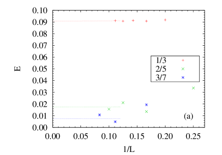
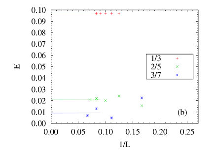
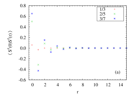
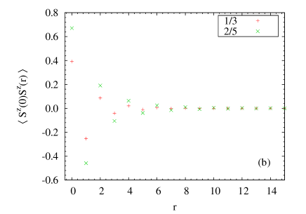
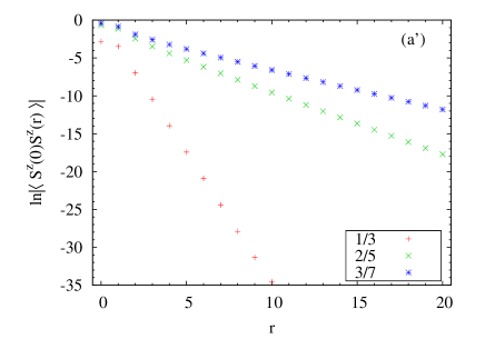
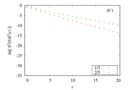
Figure 2: Energy gaps of the original FQH systems (a), and those of the corresponding effective spin chains (b). $L$ is the system size which describes the number of electrons in FQH systems ($L/\nu=15\sim 27,10\sim 25,14\sim 28$ for $\nu=1/3,2/5,3/7$) and the number of spins in effective spin chains ($L=8\sim 12,6\sim 14,6\sim 15$).

Figure 3: Correlation functions of the effective spin chains with (a) and without (b) static terms obtained by iTEBD, while (a’) and (b’) are their logarithms. $S^{z}(n)$ is the total spin of the $n$-th unit cell $S^{z}(n)=\sum_{j=np+1}^{(n+1)p}\hat{S}^{z}_{j,n}$. $r$ denotes the distance between two total spins where the lengths of unit cells are set to be unity.

Filling factor $\nu$ of the original system	Correlation length $\xi$
$1/3$	$0.29$
$2/5$	$1.10$
$3/7$	$1.63$

Table 2: Correlation length of the spin-spin corelation function of the effective spin chains. The lengths of unit cells are set to be unity.

IV Numerical analysis

In order to confirm the validity of our spin mapping of the FQH state, we numerically calculate energy gaps of $\nu=1/3,2/5,3/7$ FQH states on a torus with $L_{1}=5.3$. The energy gaps of the finite systems with the Trugman-Kivelson-type potential are obtained by exact diagonalization, and extrapolation to the infinite-size system is done using the minimum-square method. The energy gaps of the corresponding spin chains are also calculated in a similar way. As shown in Fig. 3, we find that the energy gaps of the effective spin chains and the original FQH systems decrease with increasing $p$. We should note that energy gaps in the effective spin Hamiltonian do not always correspond with those in the original systems, since the Hirbert space is limited. However, these gaps give upper bounds of the original gaps, at least.

We also calculate the correlation function $\braket{S^{z}(0)S^{z}(n)}$ of the total spins of the unit cell $S^{z}(n)=\sum_{j=np+1}^{(n+1)p}\hat{S}^{z}_{j,n}$ of the effective spin chains using iTEBD Vidal (see Fig. 3). This numerical method enables us to calculate correlation functions in infinite-size systems without extrapolations. From Fig. 3, we can read off that the correlation functions vanish exponentially as functions of the distances, regardless of whether the effective Hamiltonian includes the static terms or not. As shown in Table 2 the correlation length of the effective spin model for the $\nu=p/(2p+1)$ FQH state, $\xi$, where the length of a unit cell set to be unity, increases as $p$ increases. These properties of energy gaps and correlation functions are similar to those of the integer-$S$ quantum spin chain where the Haldane gaps decrease and correlation lengths increase as $S$ is increased.

V Conclusion and Discussion

We have shown that FQH states in $m=1$ Jain series, filling factor $\nu=p/(2p+1)$ and $\nu=p+1/(2p+1)$, beyond the thin-torus limit can be mapped to $S=1$ effective spin chains with $p$ sites in a unit cell. By numerically analyzing the energy gaps and the correlation lengths, we have shown that those effective spin chains and the original systems behave similarly in their $p$ dependence. From these results, we point out that these effective spin chains have similar properties to those of $S=p$ integer Heisenberg chains with Haldane gaps which decease as $S$ is increased. The above results give one of the explanations regarding the relationship of the hierarchy of FQH states and Haldane conjecture on the quantum spin chains.

In the present spin-mapping for $\nu=p/(2p+1)$, it was essential that the most relevant pair hopping process is given only by $\hat{V}_{21}$. Therefore, the Laughlin series $\nu=1/q$ with $q\geq 5$ cannot be treated in the same way, where contribution from the longer range hopping terms are important. Analysis for these states will be discussed elsewhere.Wang-N

VI Acknowledgment

We thank Emil J. Bergholtz for many helpful discussions. M. N. and Z.-Y. W. acknowledge support from the Global Center of Excellence Program “Nanoscience and Quantum Physics” of the Tokyo Institute of Technology. M. N. also acknowledges support from Grant-in-Aid No.23540362 by MEXT.

Appendix A Proof of Eq. (10)

Let us show that the all states in our model are generated from the root state $\ket{\Psi_{r}}$ by applying only $\hat{U}_{j}$ defined by (8) without using $\hat{U}_{j}^{\dagger}$, as written in (10). From Eq. (9), a configuration is supposed to be written as

$$\ket{\Psi_{[\bar{k},j,\cdots]}}=\hat{U}_{k}^{\dagger}\hat{U}_{j}\cdots\ket{\Psi_{r}},$$ (26)

where the parts $\cdots$ are the products of $\hat{U}$. The following conditions for operator $\hat{U}_{j}$ can be confirmed with simple calculations,

$$\hat{U}_{k}^{\dagger}\hat{U}_{j}=0,\quad\left(|k-j|\leq 2\right),$$ (27a)

$$[\hat{U}_{k}^{\dagger},\hat{U}_{j}]=0,\quad\left(|k-j|>3\right).$$ (27b)

Due to the space inversion symmetry, we only need to consider the nonvanishing case ($k-j=3$). We get

$$\hat{U}_{j+3}^{\dagger}\hat{U}_{j}=\hat{c}_{j+3}^{\dagger}\hat{c}_{j+6}^{\dagger}\hat{c}_{j+1}^{\dagger}\hat{c}_{j+2}^{\dagger}\hat{c}_{j+5}^{\mathstrut}\hat{c}_{j+4}^{\mathstrut}\hat{c}_{j+3}^{\mathstrut}\hat{c}_{j}^{\mathstrut}\;.$$ (28)

Since $\cdots\ket{\Psi_{r}}\neq\ket{\cdots 111\cdots}$ in Eq. (26), $\hat{U}_{j+3}^{\dagger}\hat{U}_{j}\cdots\ket{\Psi_{r}}$ vanishes. Thus the above lemma has been proven.

Appendix B Proof of Eq. (15)

To prove the property described by Eq. (15), we need the following lemma in a system with periodic or open boundary conditions:

$$\cdots\hat{U}_{k+1}\cdots\hat{U}_{k}\cdots=\cdots\hat{U}_{k}\cdots\hat{U}_{k+1}\cdots=0,$$ (29)

where $\cdots$ means products of $\hat{U}_{i}$. Since only $\hat{U}_{j-3}$ and $\hat{U}_{j+2p_{s}+2}$ may reduce the number of particles in the underlined part of Eq. (LABEL:root), we consider a case when one particle goes out from the unit cell by operating $\hat{U}_{j-3}$. This situation is possible when a particle is located on the $j$-th site,

$$\ket{\Psi}=\ket{\cdots 0\underline{\overset{j}{1}\cdots}\cdots}\;.$$ (30)

This state is generated after $\hat{U}_{j-2}$ or $\hat{U}_{j-1}$ has been operated to $\ket{\Psi_{r}}$. Since $\hat{U}_{j-1}$ increases the number of particles in the underlined part, we should only consider the case

$$\ket{\Psi}=\cdots\hat{U}_{j-3}\cdots\hat{U}_{j-2}\cdots\ket{\Psi_{r}}.$$ (31)

Now let us prove our lemma (29). We suppose $N_{s}$ to be the number of sites in the current system and $|k-j|<N_{s}$. The operator $\hat{U}_{j}$ defined in (8) has the following properties which can be confirmed with simple calculations:

$$\hat{U}_{j}\hat{U}_{k} =\hat{U}_{k}\hat{U}_{j},\quad\left(|k-j|\neq 2\right),$$ (32a)

$$\hat{U}_{j}\hat{U}_{k} =0,\quad\left(4>|k-j|\neq 2\right),$$ (32b)

$$\hat{U}_{j}\hat{U}_{k}\hat{U}_{j} =0,$$ (32c)

and

$$\hat{U}_{j}\hat{U}_{j+2} \cdots\hat{U}_{j+2n}$$

$$\qquad= \hat{n}_{j+2}(n_{j+3}-1)\cdots\hat{n}_{j+2n}(\hat{n}_{j+2n+1}-1)$$

$$\times\hat{c}_{j}^{\mathstrut}\hat{c}^{\dagger}_{j+1}\hat{c}^{\dagger}_{j+2n+2}\hat{c}_{j+2n+3}^{\mathstrut},$$ (33a)

$$\hat{U}_{j+2n} \cdots\hat{U}_{j+2}\hat{U}_{j}$$

$$\qquad= \hat{n}_{j+2n+1}(\hat{n}_{j+2n}-1)\cdots\hat{n}_{j+3}(\hat{n}_{j+2}-1)$$

$$\times\hat{c}_{j+2n+3}^{\mathstrut}\hat{c}^{\dagger}_{j+2n+2}\hat{c}^{\dagger}_{j+1}\hat{c}_{j}^{\mathstrut}.$$ (33b)

We find the following condition in the systems with periodic or open boundary conditions:

$$\cdots\hat{U}_{k+1}\underline{\cdots}\hat{U}_{k}\cdots=\cdots\hat{U}_{k}\underline{\cdots}\hat{U}_{k+1}\cdots=0,$$ (34)

where the underlined parts do not include $\hat{U}_{k},\hat{U}_{k+1},\hat{U}_{k-1}$, and $\hat{U}_{k+2}$. In other words, if we operate both $\hat{U}_{k}$ and $\hat{U}_{k+1}$ to $\ket{\Psi_{r}}$, then it vanishes. Let us prove this lemma. Because of the space inversion symmetry, we only need to prove the condition $\cdots\hat{U}_{k+1}\underline{\cdots}\hat{U}_{k}\cdots=0$. When the system has open boundary conditions, we just need to consider the following case:

$$\begin{split}&[\hat{U}_{k},\hat{U}_{l}]=0\;(k\neq l\pm 2)\Rightarrow\\ &[\hat{U}_{2s},\hat{U}_{2t+1}]=0\;(s,t\in\mathbb{Z};\;|2s-2t-1|<N_{s}),\end{split}$$ (35)

where Eq. (32) has been used. It is obvious that the operators $\hat{U}_{k}$ with even $k$ and $\hat{U}_{l}$ with odd $l$ commute each other, so that for the operators $\hat{U}$ in the underlined part, we can move all $\hat{U}_{k+\mathrm{odd}}$ to the right of $\hat{U}_{k}$ and all $\hat{U}_{k+\mathrm{even}}$ to the left of $\hat{U}_{k+1}$. Then we can change the order of $\hat{U}$ in the following way:

$$\cdots\hat{U}_{k+1}\underline{\cdots}\hat{U}_{k}\cdots=\cdots\hat{U}_{k+1}\hat{U}_{k}\cdots=0.$$ (36)

Then it follows from Eq. (32b) that (29) has been proven for open boundary systems.

For periodic boundary systems, we have to consider the relation $\hat{U}_{k}=\hat{U}_{k+\lambda N_{s}}$ with $\lambda\in\mathbb{Z}$. If $N_{s}$ is even, we can get Eq. (36) in a similar way of the open boundary systems. On the other hand, if $N_{s}$ is odd ($N_{s}=2M-1,\;M\in\mathbb{N}$), we consider the following approach. First, we verify the following relation which is non-trivial in this case:

$$[\hat{U}_{k},\hat{U}_{k+2n}]=0,\;(2\leq n\leq N_{s}).$$ (37)

For $2\leq n\leq(N_{s}-1)/2$, this relation can be obtained from Eq. (32). For $(N_{s}-1)/2<n\leq N_{s}$, it follows from the relation $\hat{U}_{k+2n}=\hat{U}_{k+2(n-M)+1}$ that the indices of $\hat{U}$ are always odd and less than $N_{s}$. Therefore Eq. (37) is satisfied from Eq. (32). Second, it follows from Eq. (33) that the following relation is satisfied for $n\geq M$:

$$\hat{U}_{k+2n}\cdots\hat{U}_{k+2}\hat{U}_{k}=\hat{U}_{k-2n}\cdots\hat{U}_{k-2}\hat{U}_{k}=0.$$ (38)

Using Eqs. (37) and (38), if $\underline{\cdots}\hat{U}_{k}\cdots$ is not 0, the operators $\hat{U}_{k-2s}\cdots\hat{U}_{k-4}\hat{U}_{k-2}$ in the underlined part can be moved to the left side of $\hat{U}_{k}$ as

$$\underline{\cdots}\hat{U}_{k}\cdots=$$ (39)

$$(\hat{U}_{k-2s}\cdots\hat{U}_{k-4}\hat{U}_{k-2})\hat{U}_{k}(\mbox{remaining $\hat{U}$ in}\underline{\cdots})\cdots,$$

where $0\leq s<M$. Finally, we consider the case $\cdots\hat{U}_{k+1-\lambda N_{s}}\underline{\cdots}\hat{U}_{k}\cdots\neq\cdots\hat{U}_{k+1-\lambda N_{s}}\hat{U}_{k}\cdots=\cdots\hat{U}_{k+1}\hat{U}_{k}\cdots=0$. Comparing Eq. (39) with $\cdots\hat{U}_{k+1-\lambda N_{s}}\underline{\cdots}\hat{U}_{k}\cdots$, the relation among $s,\lambda,$ and $N_{s}$ should be

$$2s=\lambda N_{s}-1.$$ (40)

Since $N_{s}$ is odd, $\lambda$ is also odd. Therefore $s\geq M$, and Eq. (38) yields $\cdots\hat{U}_{k+1}\underline{\cdots}\hat{U}_{k}\cdots=0$. Thus the lemma (29) has been proven for all cases.

The lemma (29) can also be easily proven by using the apagogical argument which assumes that one particle cannot move two sites in one direction from the initial condition.

References

• (1) K. v. Klitzing, G. Dorda, and M. Pepper Phys. Rev. Lett. 45, 494 (1980); D. C. Tsui, H. L. Stormer, and A. C. Gossard, ibid. 48, 1559 (1982).
• (2) R. B. Laughlin, Phys. Rev. B 45, 5632 (1981).
• (3) F. D. M. Haldane, Phys. Rev. Lett. 51, 605 (1983).
• (4) B. I. Halperin, Phys. Rev. Lett. 52, 1583 (1984).
• (5) J. K. Jain, Phys. Rev. Lett. 63, 199 (1989).
• (6) G. Moore, and N. Read, Nucl. Phys. B 360, 362 (1991).
• (7) X. Du, I. Skachko, F. Duerr, A. Luican, and E. Y. Andrei, Nature (London) 462, 192 (2009); K. I. Bolotin, F. Ghahari, M. D. Shulman, H. L. Stormer, and P. Kim, ibid 462, 196 (2009).
• (8) C. Nayak, S. H. Simon, A. Stern, M. Freedman, and S. Das Sarma, Rev. Mod. Phys. 80, 1083 (2008).
• (9) N. K. Wilkin, J. M. F. Gunn, and R. A. Smith Phys. Rev. Lett. 80, 2265 (1998); N. R. Cooper and N. K. Wilkin, Phys. Rev. B 60, R16279 (1999); N. Regnault and Th. Jolicoeur, Phys. Rev. Lett. 91, 030402 (2003); Y.-J. Lin, R. L. Compton, K. Jiménez-García, J. V. Porto, and I. B. Spielman, Nature 462, 628 (2009).
• (10) S. M. Girvin and D. P. Arovas, Physica Scripta. T 27, 156 (1989).
• (11) F. D. M. Haldane, Phys. Lett. 93A, 464 (1983); Phys. Rev. Lett. 50, 1153 (1983).
• (12) R. Tao and D. J. Thouless, Phys. Rev. B 28, 1142 (1983).
• (13) E. J. Bergholtz and A. Karlhede, Phys. Rev. Lett. 94, 026802 (2005).
• (14) A. Seidel, H. Fu, D. -H. Lee, J. M. Leinaas, and J. Moore, Phys. Rev. Lett. 95, 266405 (2005).
• (15) E. H. Rezayi and F. D. M. Haldane, Phys. Rev. B 50, 17199 (1994).
• (16) E. J. Bergholtz and A. Karlhede, J. Stat. Mech. L04001 (2006); Phys. Rev. B 77, 155308 (2008).
• (17) S. Jansen, E. H. Lieb, and R. Seiler, Commun. Math. Phys. 285, 503 (2009).
• (18) M. Nakamura, Z.-Y. Wang, and E. J. Bergholtz, J. Phys.: Conf. Ser. 302, 012020 (2011).
• (19) M. Nakamura, E. J. Bergholtz, and J. Suorsa, Phys. Rev. B 81, 165102 (2010).
• (20) E. J. Bergholtz, M. Nakamura, and J. Suorsa, Physica E 43, 755 (2011).
• (21) M. Nakamura, Z.-Y. Wang, and E. J. Bergholtz, Phys. Rev. Lett. 109, 016401 (2012).
• (22) S. A. Trugman and S. Kivelson, Phys. Rev. B 31, 5280 (1985).
• (23) G. Vidal, Phys. Rev. Lett. 98, 070201 (2007).
• (24) Z.-Y. Wang and M. Nakamura, arXiv:1206.3071.