Electronic properties of monolayer and bilayer graphene

Abstract

The tight-binding model of electrons in graphene is reviewed. We derive low-energy Hamiltonians supporting massless Dirac-like chiral fermions and massive chiral fermions in monolayer and bilayer graphene, respectively, and we describe how their chirality is manifest in the sequencing of plateaus observed in the integer quantum Hall effect. The opening of a tuneable band gap in bilayer graphene in response to a transverse electric field is described, and we explain how Hartree theory may be used to develop a simple analytical model of screening.

0.1 Introduction

More than sixty years ago, Wallace wallace46 modeled the electronic band structure of graphene. Research into graphene was stimulated by interest in the properties of bulk graphite because, from a theoretical point of view, two-dimensional graphene serves as a building block for the three-dimensional material. Following further work, the tight-binding model of electrons in graphite, that takes into account coupling between layers, became known as the Slonczewski-Weiss-McClure model sw58 ; mcclure57 ; dressel02 . As well as serving as the basis for models of carbon-based materials including graphite, buckyballs, and carbon nanotubes d+m84 ; gon92 ; a+a93 ; k+m97 ; ando98 ; mceuen99 ; saito , the honeycomb lattice of graphene has been used theoretically to study Dirac fermions in a condensed matter system semenoff84 ; haldane88 . Since the experimental isolation of individual graphene flakes novo04 , and the observation of the integer quantum Hall effect in monolayers novo05 ; zhang05 and bilayers novo06 , there has been an explosion of interest in the behavior of chiral electrons in graphene.

This Chapter begins in Sect. 0.2 with a description of the crystal structure of monolayer graphene. Section 0.3 briefly reviews the tight-binding model of electrons in condensed matter materials ash+mer ; saito , and Sect. 0.4 describes its application to monolayer graphene saito ; cnreview ; bena09 . Then, in Section 0.5, we explain how a Dirac-like Hamiltonian describing massless chiral fermions emerges from the tight-binding model at low energy. The tight-binding model is applied to bilayer graphene in Sect. 0.6, and Sect. 0.7 describes how low-energy electrons in bilayers behave as massive chiral quasiparticles novo06 ; mcc06a . In Sect. 0.8, we describe how the chiral Hamiltonians of monolayer and bilayer graphene corresponding to Berry’s phase $\pi$ and $2\pi$, respectively, have associated four- and eight-fold degenerate zero-energy Landau levels, leading to an unusual sequence of plateaus in the integer quantum Hall effect novo05 ; zhang05 ; novo06 .

Section 0.9 discusses an additional contribution to the low-energy Hamiltonians of monolayer and bilayer graphene, known as trigonal warping dressel02 ; dre74 ; nak76 ; ino62 ; gup72 ; ando98 ; mcc06a , that produces a Liftshitz transition in the band structure of bilayer graphene at low energy. Finally, Sect. 0.10 describes how an external transverse electric field applied to bilayer graphene, due to doping or gates, may open a band gap that can be tuned between zero up to the value of the interlayer coupling, around three to four hundred meV mcc06a ; ohta06 ; oostinga . Hartree theory and the tight-binding model are used to develop a simple model of screening by electrons in bilayer graphene in order to calculate the density dependence of the band gap mcc06b .

0.2 The crystal structure of monolayer graphene

0.2.1 The real space structure

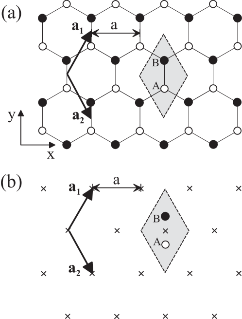
Figure 1: (a) The honeycomb crystal structure of monolayer graphene where white (black) circles indicate carbon atoms on $A$ ($B$) sites and straight lines indicate $\sigma$ bonds between them. Vectors $\mathbf{a}_{1}$ and $\mathbf{a}_{2}$ are primitive lattice vectors of length equal to the lattice constant $a$. The shaded rhombus is a unit cell containing two atoms, one $A$ and one $B$. (b) Crosses indicate lattice points of the hexagonal Bravais lattice. The honeycomb structure in (a) consists of the hexagonal Bravais lattice [shown in (b)] with a basis of two atoms, one $A$ and one $B$, at each lattice point.

Monolayer graphene consists of carbon atoms arranged with a two-dimensional honeycomb crystal structure as shown in Fig. 1(a). The honeycomb structure ash+mer ; saito consists of the hexagonal Bravais lattice, Fig. 1(b), with a basis of two atoms, labeled $A$ and $B$, at each lattice point.

Throughout this Chapter, we use a Cartesian coordinate system with $x$ and $y$ axes in the plane of the graphene crystal, and a $z$ axis perpendicular to the graphene plane. Two-dimensional vectors in the same plane as the graphene are expressed solely in terms of their $x$ and $y$ coordinates, so that, for example, the primitive lattice vectors of the hexagonal Bravais lattice, Fig. 1(b), are $\mathbf{a}_{1}$ and $\mathbf{a}_{2}$ where

$$\mathbf{a}_{1}=\left(\frac{a}{2},\frac{\sqrt{3}a}{2}\right)\,,\qquad\mathbf{a}_{2}=\left(\frac{a}{2},-\frac{\sqrt{3}a}{2}\right)\,,$$ (1)

and $a=|\mathbf{a}_{1}|=|\mathbf{a}_{2}|$ is the lattice constant. In graphene, $a=2.46\,$Åsaito . The lattice constant is the distance between unit cells, whereas the distance between carbon atoms is the carbon-carbon bond length $a_{CC}=a/\sqrt{3}=1.42\,$Å. Note that the honeycomb structure is not a Bravais lattice because atomic positions $A$ and $B$ are not equivalent: it is not possible to connect them with a lattice vector $\mathbf{R}=n_{1}\mathbf{a}_{1}+n_{2}\mathbf{a}_{2}$ where $n_{1}$ and $n_{2}$ are integers. Taken alone, the $A$ atomic positions (or, the $B$ atomic positions) make up an hexagonal Bravais lattice and, in the following, we will often refer to them as the ‘$A$ sublattice’ (or, the ‘$B$ sublattice’).

0.2.2 The reciprocal lattice of graphene

Primitive reciprocal lattice vectors $\mathbf{b}_{1}$ and $\mathbf{b}_{2}$ satisfying $\mathbf{a}_{1}\mathbf{b}_{1}=\mathbf{a}_{2}\mathbf{b}_{2}=2\pi$ and $\mathbf{a}_{1}\mathbf{b}_{2}=\mathbf{a}_{2}\mathbf{b}_{1}=0$ are given by

$$\mathbf{b}_{1}=\left(\frac{2\pi}{a},\frac{2\pi}{\sqrt{3}a}\right)\,,\qquad\mathbf{b}_{2}=\left(\frac{2\pi}{a},-\frac{2\pi}{\sqrt{3}a}\right)\,.$$ (2)

The resulting reciprocal lattice is shown in Fig. 2, which is an hexagonal Bravais lattice. The first Brillouin zone is hexagonal, as indicated by the shaded region in Fig. 2.

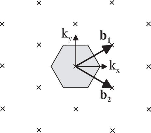
Figure 2: The reciprocal lattice of monolayer graphene where crosses indicate reciprocal lattice points, and vectors $\mathbf{b}_{1}$ and $\mathbf{b}_{2}$ are primitive lattice vectors. The shaded hexagon indicates the first Brillouin zone.

0.2.3 The atomic orbitals of graphene

Each carbon atom has six electrons, of which two are core electrons and four are valence electrons. The latter occupy $2s$, $2p_{x}$, $2p_{y}$, and $2p_{z}$ orbitals. In graphene, the orbitals are $sp^{2}$ hybridized, meaning that two of the $2p$ orbitals, the $2p_{x}$ and $2p_{y}$ that lie in the graphene plane, mix with the $2s$ orbital to form three $sp^{2}$ hybrid orbitals per atom, each lying in the graphene plane and oriented $120^{\circ}$ to each other saito . They form $\sigma$ bonds with other atoms, shown as straight lines in the honeycomb crystal structure, Fig. 1(a). The remaining $2p_{z}$ orbital for each atom lies perpendicular to the plane, and, when combined with the $2p_{z}$ orbitals on adjacent atoms in graphene, forms a $\pi$ orbital. Electronic states close to the Fermi level in graphene are described well by a model taking into account only the $\pi$ orbital, meaning that the tight-binding model can include only one electron per atomic site, in a $2p_{z}$ orbital.

0.3 The tight-binding model

We begin by presenting a general description of the tight-binding model for a system with $n$ atomic orbitals $\phi_{j}$ in the unit cell, labeled by index $j=1\ldots n$. Further details may be found in the book by Saito, Dresselhaus, and Dresselhaus saito . It is assumed that the system has translational invariance. Then, the model may be written using $n$ different Bloch functions $\Phi_{j}(\mathbf{k},\mathbf{r})$ that depend on the position vector $\mathbf{r}$ and wave vector $\mathbf{k}$. They are given by

$$\Phi_{j}(\mathbf{k},\mathbf{r})=\frac{1}{\sqrt{N}}\sum_{i=1}^{N}e^{i\mathbf{k}.\mathbf{R}_{j,i}}\phi_{j}\left(\mathbf{r}-\mathbf{R}_{j,i}\right)\,,$$ (3)

where the sum is over $N$ different unit cells, labeled by index $i=1\ldots N$, and $\mathbf{R}_{j,i}$ denotes the position of the $j$th orbital in the $i$th unit cell.

In general, an electronic wave function $\Psi_{j}(\mathbf{k},\mathbf{r})$ is given by a linear superposition of the $n$ different Bloch functions,

$$\Psi_{j}(\mathbf{k},\mathbf{r})=\sum_{l=1}^{n}{c}_{j,l}(\mathbf{k})\,\Phi_{l}(\mathbf{k},\mathbf{r})\,,$$ (4)

where ${c}_{j,l}$ are coefficients of the expansion. The energy $E_{j}(\mathbf{k})$ of the $j$th band is given by

$$E_{j}(\mathbf{k})=\frac{\langle\Psi_{j}|{\cal H}|\Psi_{j}\rangle}{\langle\Psi_{j}|\Psi_{j}\rangle}\,,$$ (5)

where ${\cal H}$ is the Hamiltonian. Substituting the expansion of the wave function (4) into the energy gives

$$E_{j}(\mathbf{k}) = \frac{\sum_{i,l}^{n}{c}_{ji}^{\ast}{c}_{jl}\langle\Phi_{i}|{\cal H}|\Phi_{l}\rangle}{\sum_{i,l}^{n}{c}_{ji}^{\ast}{c}_{jl}\langle\Phi_{i}|\Phi_{l}\rangle}\,,$$ (6)

$$= \frac{\sum_{i,l}^{n}H_{il}{c}_{ji}^{\ast}{c}_{jl}}{\sum_{i,l}^{n}S_{il}{c}_{ji}^{\ast}{c}_{jl}}\,,$$ (7)

where transfer integral matrix elements $H_{il}$ and overlap integral matrix elements $S_{il}$ are defined by

$$H_{il}=\langle\Phi_{i}|{\cal H}|\Phi_{l}\rangle\,,\qquad S_{il}=\langle\Phi_{i}|\Phi_{l}\rangle\,.$$ (8)

We minimize the energy $E_{j}$ with respect to the coefficient ${c}_{jm}^{\ast}$ by calculating the derivative,

$$\frac{\partial E_{j}}{\partial{c}_{jm}^{\ast}}=\frac{\sum_{l}^{n}H_{ml}{c}_{jl}}{\sum_{i,l}^{n}S_{il}{c}_{ji}^{\ast}{c}_{jl}}-\frac{\sum_{i,l}^{n}H_{il}{c}_{ji}^{\ast}{c}_{jl}\sum_{l}^{n}S_{ml}{c}_{jl}}{\left(\sum_{i,l}^{n}S_{il}{c}_{ji}^{\ast}{c}_{jl}\right)^{2}}\,.$$ (9)

The second term contains a factor equal to the energy $E_{j}$ itself, (7). Then, setting $\partial E_{j}/\partial{c}_{jm}^{\ast}=0$ and omitting the common factor $\sum_{i,l}^{n}S_{il}{c}_{ji}^{\ast}{c}_{jl}$ gives

$$\sum_{l=1}^{n}H_{ml}{c}_{jl}=E_{j}\sum_{l=1}^{n}S_{ml}{c}_{jl}\,.$$ (10)

This can be written as a matrix equation. Consider the specific example of two orbitals per unit cell, $n=2$. Then, we can select the possible values of $m$ (either $m=1$ or $m=2$) and write out the summation in (10) explicitly:

$$m=1\quad\Rightarrow\quad H_{11}{c}_{j1}+H_{12}{c}_{j2} = E_{j}\left(S_{11}{c}_{j1}+S_{12}{c}_{j2}\right)\,,$$ (11)

$$m=2\quad\Rightarrow\quad H_{21}{c}_{j1}+H_{22}{c}_{j2} = E_{j}\left(S_{21}{c}_{j1}+S_{22}{c}_{j2}\right)\,.$$ (12)

These two equations may be combined into a matrix equation,

$$\left(\begin{array}[]{cc}H_{11}&H_{12}\\ H_{21}&H_{22}\\ \end{array}\right)\left(\begin{array}[]{c}{c}_{j1}\\ {c}_{j2}\\ \end{array}\right) = E_{j}\left(\begin{array}[]{cc}S_{11}&S_{12}\\ S_{21}&S_{22}\\ \end{array}\right)\left(\begin{array}[]{c}{c}_{j1}\\ {c}_{j2}\\ \end{array}\right)\,.$$ (21)

For general values of $n$, defining $H$ as the transfer integral matrix, $S$ as the overlap integral matrix and $\psi_{j}$ as a column vector,

$$\!\!\!\!\!\!\!\!\!\!\!\!H=\left(\begin{array}[]{cccc}H_{11}&H_{12}&\cdots&H_{1n}\\ H_{21}&H_{22}&\cdots&H_{2n}\\ \vdots&\vdots&\ddots&\vdots\\ H_{n1}&H_{n2}&\cdots&H_{nn}\\ \end{array}\right)\!\!,\,S=\left(\begin{array}[]{cccc}S_{11}&S_{12}&\cdots&S_{1n}\\ S_{21}&S_{22}&\cdots&S_{2n}\\ \vdots&\vdots&\ddots&\vdots\\ S_{n1}&S_{n2}&\cdots&S_{nn}\\ \end{array}\right)\!\!,\,\psi_{j}=\left(\begin{array}[]{c}{c}_{j1}\\ {c}_{j2}\\ \vdots\\ {c}_{jn}\\ \end{array}\right)\!\!,$$ (34)

allows the relation (10) to be expressed as

$$H\psi_{j} = E_{j}S\psi_{j}\,.$$ (35)

The energies $E_{j}$ may be determined by solving the secular equation

$$\det\left(H-E_{j}S\right)=0\,,$$ (36)

once the transfer integral matrix $H$ and the overlap integral matrix $S$ are known. Here, ‘$\det$’ stands for the determinant of the matrix. In the following, we will omit the subscript $j=1\ldots n$ in (35),(36), bearing in mind that the number of solutions is equal to the number of different atomic orbitals per unit cell.

0.4 The tight-binding model of monolayer graphene

We apply the tight-binding model described in Sect. 0.3 to monolayer graphene, taking into account one $2p_{z}$ orbital per atomic site. As there are two atoms in the unit cell of graphene, labeled $A$ and $B$ in Fig. 1, the model includes two Bloch functions, $n=2$. For simplicity, we replace index $j=1$ with $j=A$, and $j=2$ with $j=B$. Now we proceed to determine the transfer integral matrix $H$ and the overlap integral matrix $S$.

0.4.1 Diagonal matrix elements

Substituting the expression for the Bloch function (3) into the definition of the transfer integral (8) allows us to write the diagonal matrix element corresponding to the $A$ sublattice as

$$\!\!\!\!\!\!H_{AA}=\frac{1}{N}\sum_{i=1}^{N}\sum_{j=1}^{N}e^{i\mathbf{k}.\left(\mathbf{R}_{A,j}-\mathbf{R}_{A,i}\right)}\langle\phi_{A}\left(\mathbf{r}-\mathbf{R}_{A,i}\right)|{\cal H}|\phi_{A}\left(\mathbf{r}-\mathbf{R}_{A,j}\right)\rangle,$$ (37)

where $\mathbf{k}=(k_{x},k_{y})$ is the wave vector in the graphene plane. Equation (37) includes a double summation over all the $A$ sites of the lattice. If we assume that the dominant contribution arises from the same site $j=i$ within every unit cell, then:

$$H_{AA}\approx\frac{1}{N}\sum_{i=1}^{N}\langle\phi_{A}\left(\mathbf{r}-\mathbf{R}_{A,i}\right)|{\cal H}|\phi_{A}\left(\mathbf{r}-\mathbf{R}_{A,i}\right)\rangle\,,$$ (38)

The matrix element $\langle\phi_{A}|{\cal H}|\phi_{A}\rangle$ within the summation has the same value on every $A$ site, i.e. it is independent of the site index $i$. We set it to be equal to a parameter

$$\epsilon_{2p}=\langle\phi_{A}\left(\mathbf{r}-\mathbf{R}_{A,i}\right)|{\cal H}|\phi_{A}\left(\mathbf{r}-\mathbf{R}_{A,i}\right)\rangle\,,$$ (39)

that is equal to the energy of the $2p_{z}$ orbital. Then, keeping only the same site contribution,

$$H_{AA}\approx\frac{1}{N}\sum_{i=1}^{N}\epsilon_{2p}=\epsilon_{2p}\,.$$ (40)

It is possible to take into account the contribution of other terms in the double summation (37), such as next-nearest neighbor contributions sasaki ; peres06 . They generally have a small effect on the electronic band structure and will not be discussed here. The $B$ sublattice has the same structure as the $A$ sublattice, and the carbon atoms on the two sublattices are chemically identical. This means that the diagonal transfer integral matrix element corresponding to the $B$ sublattice has the same value as that of the $A$ sublattice:

$$H_{BB}=H_{AA}\approx\epsilon_{2p}\,.$$ (41)

A calculation of the diagonal elements of the overlap integral matrix proceeds in a similar way as for those of the transfer integral. In this case, the overlap between a $2p_{z}$ orbital on the same atom is equal to unity,

$$\langle\phi_{A}\left(\mathbf{r}-\mathbf{R}_{A,i}\right)|\phi_{A}\left(\mathbf{r}-\mathbf{R}_{A,i}\right)\rangle=1\,.$$ (42)

Then, assuming that the same site contribution dominates,

$$S_{AA} = \frac{1}{N}\sum_{i=1}^{N}\sum_{j=1}^{N}e^{i\mathbf{k}.\left(\mathbf{R}_{A,j}-\mathbf{R}_{A,i}\right)}\langle\phi_{A}\left(\mathbf{r}-\mathbf{R}_{A,i}\right)|\phi_{A}\left(\mathbf{r}-\mathbf{R}_{A,j}\right)\rangle\,,$$ (43)

$$\approx \frac{1}{N}\sum_{i=1}^{N}\langle\phi_{A}\left(\mathbf{r}-\mathbf{R}_{A,i}\right)|\phi_{A}\left(\mathbf{r}-\mathbf{R}_{A,i}\right)\rangle\,,$$ (44)

$$= \frac{1}{N}\sum_{i=1}^{N}1$$ (45)

$$= 1\,.$$ (46)

Again, as the $B$ sublattice has the same structure as the $A$ sublattice,

$$S_{BB}=S_{AA}=1\,.$$ (47)

0.4.2 Off-diagonal matrix elements

Substituting the expression for the Bloch function (3) into the definition of the transfer integral (8) allows us to write an off-diagonal matrix element as

$$\!\!\!\!\!\!H_{AB}=\frac{1}{N}\sum_{i=1}^{N}\sum_{j=1}^{N}e^{i\mathbf{k}.\left(\mathbf{R}_{B,j}-\mathbf{R}_{A,i}\right)}\langle\phi_{A}\left(\mathbf{r}-\mathbf{R}_{A,i}\right)|{\cal H}|\phi_{B}\left(\mathbf{r}-\mathbf{R}_{B,j}\right)\rangle.$$ (48)

It describes processes of hopping between the $A$ and $B$ sublattices, and contains a summation over all the $A$ sites ($i=1\ldots N$) at positions $\mathbf{R}_{A,i}$ and all the $B$ sites ($j=1\ldots N$) at $\mathbf{R}_{B,j}$.

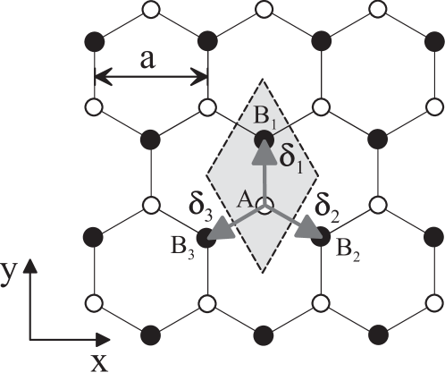
Figure 3: The honeycomb crystal structure of monolayer graphene. In the nearest-neighbor approximation, we consider hopping from an $A$ site (white) to three adjacent $B$ sites (black), labeled $B_{1}$, $B_{2}$, $B_{3}$, with position vectors $\mbox{\boldmath$\delta$}_{1}$, $\mbox{\boldmath$\delta$}_{2}$, $\mbox{\boldmath$\delta$}_{3}$, respectively, relative to the $A$ site.

In the following, we assume that the dominant contribution to the off-diagonal matrix element (48) arises from hopping between nearest neighbors only. If we focus on an individual $A$ atom, i.e. we consider a fixed value of the index $i$, we see that it has three neighboring $B$ atoms, Fig. 3, that we will label with a new index $l$ ($l=1\ldots 3$). Each $A$ atom has three such neighbors, so it is possible to write the nearest-neighbors contribution to the off-diagonal matrix element (48) as

$$\!\!\!H_{AB}\approx\frac{1}{N}\sum_{i=1}^{N}\sum_{l=1}^{3}e^{i\mathbf{k}.\left(\mathbf{R}_{B,l}-\mathbf{R}_{A,i}\right)}\langle\phi_{A}\left(\mathbf{r}-\mathbf{R}_{A,i}\right)|{\cal H}|\phi_{B}\left(\mathbf{r}-\mathbf{R}_{B,l}\right)\rangle\,.$$ (49)

The matrix element between neighboring atoms, $\langle\phi_{A}|{\cal H}|\phi_{B}\rangle$, has the same value for each neighboring pair, i.e. it is independent of indices $i$ and $l$. We set it equal to a parameter, $t=\langle\phi_{A}\left(\mathbf{r}-\mathbf{R}_{A,i}\right)|{\cal H}|\phi_{B}\left(\mathbf{r}-\mathbf{R}_{B,l}\right)\rangle$. Since $t$ is negative saito , it is common practice to express it in terms of a positive parameter $\gamma_{0}=-t$, where

$$\gamma_{0}=-\langle\phi_{A}\left(\mathbf{r}-\mathbf{R}_{A,i}\right)|{\cal H}|\phi_{B}\left(\mathbf{r}-\mathbf{R}_{B,l}\right)\rangle\,.$$ (50)

Then, we write the off-diagonal transfer integral matrix element as

$$H_{AB} \approx -\frac{1}{N}\sum_{i=1}^{N}\sum_{l=1}^{3}e^{i\mathbf{k}.\left(\mathbf{R}_{B,l}-\mathbf{R}_{A,i}\right)}\gamma_{0}\,,$$ (51)

$$= -\frac{\gamma_{0}}{N}\sum_{i=1}^{N}\sum_{l=1}^{3}e^{i\mathbf{k}.\mbox{\boldmath$\delta$}_{l}}\equiv-\gamma_{0}f\left(\mathbf{k}\right)\,,$$ (52)

$$f\left(\mathbf{k}\right) = \sum_{l=1}^{3}e^{i\mathbf{k}.\mbox{\boldmath$\delta$}_{l}}\,,$$ (53)

where the position vector of atom $B_{l}$ relative to the $A_{i}$ atom is denoted $\mbox{\boldmath$\delta$}_{l}=\mathbf{R}_{B,l}-\mathbf{R}_{A,i}$, and we used the fact that the summation over the three neighboring $B$ atoms is the same for all $A_{i}$ atoms.

For the three $B$ atoms shown in Fig. 3, the three vectors are

$$\mbox{\boldmath$\delta$}_{1}=\left(0,\frac{a}{\sqrt{3}}\right)\,,\quad\mbox{\boldmath$\delta$}_{2}=\left(\frac{a}{2},-\frac{a}{2\sqrt{3}}\right)\,,\quad\mbox{\boldmath$\delta$}_{3}=\left(-\frac{a}{2},-\frac{a}{2\sqrt{3}}\right)\,\,.$$ (54)

Note that $|\mbox{\boldmath$\delta$}_{1}|=|\mbox{\boldmath$\delta$}_{2}|=|\mbox{\boldmath$\delta$}_{3}|=a/\sqrt{3}$ is the carbon-carbon bond length. Then, the function $f\left(\mathbf{k}\right)$ describing nearest-neighbor hopping may be evaluated as

$$f\left(\mathbf{k}\right) = \sum_{l=1}^{3}e^{i\mathbf{k}.\mbox{\boldmath$\delta$}_{l}}\,,$$ (55)

$$= e^{ik_{y}a/\sqrt{3}}+e^{ik_{x}a/2}e^{-ik_{y}a/2\sqrt{3}}+e^{-ik_{x}a/2}e^{-ik_{y}a/2\sqrt{3}}\,,$$ (56)

$$= e^{ik_{y}a/\sqrt{3}}+2e^{-ik_{y}a/2\sqrt{3}}\cos\left(k_{x}a/2\right)\,.$$ (57)

The other off-diagonal matrix element $H_{BA}$ is the complex conjugate of $H_{AB}$:

$$H_{AB}\approx-\gamma_{0}f\left(\mathbf{k}\right)\,,\qquad H_{BA}\approx-\gamma_{0}f^{\ast}\left(\mathbf{k}\right)\,.$$ (58)

A calculation of an off-diagonal element of the overlap integral matrix proceeds in a similar way as for the transfer integral:

$$\!\!\!S_{AB} = \frac{1}{N}\sum_{i=1}^{N}\sum_{j=1}^{N}e^{i\mathbf{k}.\left(\mathbf{R}_{B,j}-\mathbf{R}_{A,i}\right)}\langle\phi_{A}\left(\mathbf{r}-\mathbf{R}_{A,i}\right)|\phi_{B}\left(\mathbf{r}-\mathbf{R}_{B,j}\right)\rangle,$$ (59)

$$\approx \frac{1}{N}\sum_{i=1}^{N}\sum_{l=1}^{3}e^{i\mathbf{k}.\left(\mathbf{R}_{B,l}-\mathbf{R}_{A,i}\right)}\langle\phi_{A}\left(\mathbf{r}-\mathbf{R}_{A,i}\right)|\phi_{B}\left(\mathbf{r}-\mathbf{R}_{B,l}\right)\rangle\,,$$ (60)

$$= s_{0}f\left(\mathbf{k}\right)\,,$$ (61)

where the parameter $s_{0}=\langle\phi_{A}\left(\mathbf{r}-\mathbf{R}_{A,i}\right)|\phi_{B}\left(\mathbf{r}-\mathbf{R}_{B,l}\right)\rangle$, and $S_{BA}=S_{AB}^{\ast}=s_{0}f^{\ast}\left(\mathbf{k}\right)$. The presence of non-zero $s_{0}$ takes into account the possibility that orbitals on adjacent atomic sites are not strictly orthogonal.

0.4.3 The low-energy electronic bands of monolayer graphene

Summarizing the results of this section, the transfer integral matrix elements (41) and (58), and the overlap integral matrix elements (47) and (61) give

$$H_{1}=\left(\begin{array}[]{cc}\epsilon_{2p}&-\gamma_{0}f\left(\mathbf{k}\right)\\ -\gamma_{0}f^{\ast}\left(\mathbf{k}\right)&\epsilon_{2p}\\ \end{array}\right)\,,\qquad S_{1}=\left(\begin{array}[]{cc}1&s_{0}f\left(\mathbf{k}\right)\\ s_{0}f^{\ast}\left(\mathbf{k}\right)&1\\ \end{array}\right)\,,$$ (66)

where we use the subscript ‘1’ to stress that these matrices apply to monolayer graphene. The corresponding energy $E$ may be determined by solving the secular equation $\det\left(H_{1}-ES_{1}\right)=0$, (36):

$$\det\!\left(\begin{array}[]{cc}\epsilon_{2p}-E&-\left(\gamma_{0}+Es_{0}\right)f\left(\mathbf{k}\right)\\ -\left(\gamma_{0}+Es_{0}\right)f^{\ast}\left(\mathbf{k}\right)&\epsilon_{2p}-E\\ \end{array}\right) = 0\,,$$ (69)

$$\Rightarrow\quad\left(E-\epsilon_{2p}\right)^{2}-\left(\left[E-\epsilon_{2p}\right]s_{0}+\epsilon_{2p}s_{0}+\gamma_{0}\right)^{2}|f\left(\mathbf{k}\right)|^{2} = 0\,.$$ (70)

Solving this quadratic equation yields the energy:

$$E_{\pm}=\frac{\epsilon_{2p}\pm\gamma_{0}|f\left(\mathbf{k}\right)|}{1\mp s_{0}|f\left(\mathbf{k}\right)|}\,.$$ (71)

This expression appears in Saito et al saito , where parameter values $\gamma_{0}=3.033\,$eV, $s_{0}=0.129$, $\epsilon_{2p}=0$ are quoted. The latter value ($\epsilon_{2p}=0$) means that the zero of energy is set to be equal to the energy of the $2p_{z}$ orbital. The resulting band structure $E_{\pm}$ is shown in Fig. 4 in the vicinity of the Brillouin zone. A particular cut through the band structure is shown in Fig. 5 where the bands are plotted as a function of wave vector component $k_{x}$ along the line $k_{y}=0$, a line that passes through the center of the Brillouin zone, labeled $\Gamma$, and two corners of the Brillouin zone, labeled $K_{+}$ and $K_{-}$ (see the inset of Fig. 5). The Fermi level in pristine graphene is located at zero energy. There are two energy bands, that we refer to as the conduction band ($E_{+}$) and the valence band ($E_{-}$). The interesting feature of the band structure is that there is no band gap between the conduction and valence bands. Instead the bands cross at the six corners of the Brillouin zone, Fig. 4. The corners of the Brillouin zone are known as $K$ points, and two of them are explicitly labeled $K_{+}$ and $K_{-}$ in Fig. 4. Near these points, the dispersion is linear and electronic properties may be described by a Dirac-like Hamiltonian. This will be explored in more detail in the next section. Note also that the band structure displays a large asymmetry between the conduction and valence bands that is most pronounced in the vicinity of the $\Gamma$ point. This arises from the non-zero overlap parameter $s_{0}$ appearing in (71).

The tight-binding model described here cannot be used to determine the values of parameters such as $\gamma_{0}$ and $s_{0}$. They must be determined either by an alternative theoretical method, such as density-functional theory, or by comparison of the tight-binding model with experiments. Note, however, that the main qualitative features described in this chapter do not depend on the precise values of the parameters quoted.

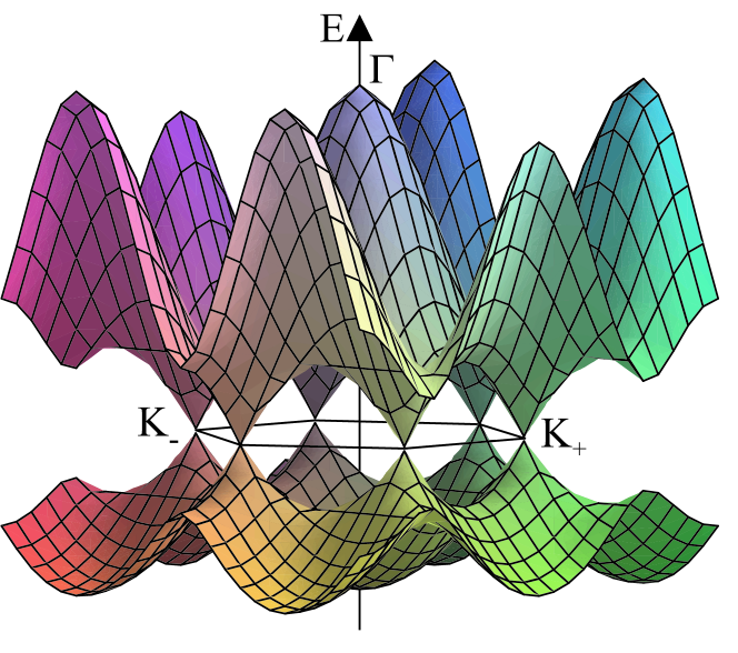
Figure 4: The low-energy band structure of monolayer graphene Eq. (71) taking into account nearest-neighbor hopping with parameter $\gamma_{0}=3.033\,$eV, nearest-neighbor overlap parameter $s_{0}=0.129$, and orbital energy $\epsilon_{2p}=0$ saito . The plot shows the bands calculated in the vicinity of the first Brillouin zone, with conduction and valence bands touching at six corners of the Brillouin zone, two of them are labeled $K_{+}$ and $K_{-}$. Label $\Gamma$ indicates the center of the Brillouin zone.

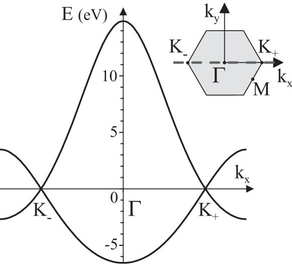
Figure 5: The low-energy band structure of monolayer graphene Eq. (71) taking into account nearest-neighbor hopping with parameter $\gamma_{0}=3.033\,$eV, nearest-neighbor overlap parameter $s_{0}=0.129$, and orbital energy $\epsilon_{2p}=0$ saito . The plot shows a cut through the band structure Fig. 4, plotted along the $k_{x}$ axis intersecting points $K_{-}$, $\Gamma$, and $K_{+}$ in the Brillouin zone, shown as the dotted line in the inset.

0.5 Massless chiral quasiparticles in monolayer graphene

0.5.1 The Dirac-like Hamiltonian

As described in the previous section, the electronic band structure of monolayer graphene, Figs. 4, 5, is gapless, with crossing of the bands at points $K_{+}$ and $K_{-}$ located at corners of the Brillouin zone. In this section, we show that electronic properties near these points may be described by a Dirac-like Hamiltonian.

Although the first Brillouin zone has six corners, only two of them are non-equivalent. In this Chapter, we choose points $K_{+}$ and $K_{-}$, Figs. 4, 5, as a non-equivalent pair. It is possible to connect two of the other corners to $K_{+}$ using a reciprocal lattice vector (hence, the other two are equivalent to $K_{+}$), and it is possible to connect the remaining two corners to $K_{-}$ using a reciprocal lattice vector (hence, the remaining two are equivalent to $K_{-}$), but it is not possible to connect $K_{+}$ and $K_{-}$ with a reciprocal lattice vector. To distinguish between $K_{+}$ and $K_{-}$, we will use an index $\xi=\pm 1$. Using the values of the primitive reciprocal lattice vectors $\mathbf{b}_{1}$ and $\mathbf{b}_{2}$, (2), it can be seen that the wave vector corresponding to point $K_{\xi}$ is given by

$$\mathbf{K}_{\xi}=\xi\left(\frac{4\pi}{3a},0\right)\,.$$ (72)

Note that the $K$ points are often called ‘valleys’ using nomenclature from semiconductor physics.

In the tight-binding model, coupling between the $A$ and $B$ sublattices is described by the off-diagonal matrix element $H_{AB}$, (58), that is proportional to parameter $\gamma_{0}$ and the function $f(\mathbf{k})$, (55). Exactly at the $K_{\xi}$ point, $\mathbf{k}=\mathbf{K}_{\xi}$, the latter is equal to

$$f\left(\mathbf{K}_{\xi}\right) = e^{0}+e^{i\xi 2\pi/3}+e^{-i\xi 2\pi/3}=0\,.$$ (73)

This indicates that there is no coupling between the $A$ and $B$ sublattices exactly at the $K_{\xi}$ point. Since the two sublattices are both hexagonal Bravais lattices of carbon atoms, they support the same quantum states, leading to a degeneracy point in the spectrum at $K_{\xi}$, Figs. 4, 5.

The exact cancelation of the three factors describing coupling between the $A$ and $B$ sublattices, (73), no longer holds when the wave vector is not exactly equal to that of the $K_{\xi}$ point. We introduce a momentum $\mathbf{p}$ that is measured from the center of the $K_{\xi}$ point,

$$\mathbf{p}=\hbar\mathbf{k}-\hbar\mathbf{K}_{\xi}\,.$$ (74)

Then, the coupling between the $A$ and $B$ sublattices is proportional to

$$f\left(\mathbf{k}\right) = e^{ip_{y}a/\sqrt{3}\hbar}+2e^{-ip_{y}a/2\sqrt{3}\hbar}\cos\left(\frac{2\pi\xi}{3}+\frac{p_{x}a}{2\hbar}\right)\,,$$ (75)

$$\approx \left(1+\frac{ip_{y}a}{\sqrt{3}\hbar}\right)+2\left(1-\frac{ip_{y}a}{2\sqrt{3}\hbar}\right)\left(-\frac{1}{2}-\frac{\xi\sqrt{3}p_{x}a}{4\hbar}\right)\,,$$ (76)

$$\approx -\frac{\sqrt{3}a}{2\hbar}\left(\xi p_{x}-ip_{y}\right)\,,$$ (77)

where we kept only linear terms in the momentum $\mathbf{p}=\left(p_{x},p_{y}\right)$, an approximation that is valid close to the $K_{\xi}$ point, i.e. for $pa/\hbar\ll 1$, where $p=|\mathbf{p}|=(p_{x}^{2}+p_{y}^{2})^{1/2}$. Using this approximate expression for the function $f\left(\mathbf{k}\right)$, the transfer integral matrix (66) in the vicinity of point $K_{\xi}$ becomes

$$H_{1,\xi}=v\left(\begin{array}[]{cc}0&\xi p_{x}-ip_{y}\\ \xi p_{x}+ip_{y}&0\\ \end{array}\right)\,.$$ (80)

Here, we used $\epsilon_{2p}=0$ saito which defines the zero of the energy axis to coincide with the energy of the $2p_{z}$ orbital. The parameters $a$ and $\gamma_{0}$ were combined into a velocity $v$ defined as $v=\sqrt{3}a\gamma_{0}/(2\hbar)$.

Within the linear-in-momentum approximation for $f\left(\mathbf{k}\right)$, (77), the overlap matrix $S_{1}$ may be regarded as a unit matrix, because its off-diagonal elements, proportional to $s_{0}$, only contribute quadratic-in-momentum terms to the energy $E_{\pm}$, (71). Since $S_{1}$ is approximately equal to a unit matrix, (35) becomes $H_{1}\psi=E\psi$, indicating that $H_{1}$, (80), is an effective Hamiltonian for monolayer graphene at low-energy. The energy eigenvalues and eigenstates of $H_{1}$ are given by

$$E_{\pm}=\pm vp\,,\qquad\psi_{\pm}=\frac{1}{\sqrt{2}}\left(\begin{array}[]{c}1\\ \pm\xi e^{i\xi\varphi}\\ \end{array}\right)e^{i\mathbf{p}.\mathbf{r}/\hbar}\,,$$ (83)

where $\pm$ refer to the conduction and valence bands, respectively. Here $\varphi$ is the polar angle of the momentum in the graphene plane, $\mathbf{p}=\left(p_{x},p_{y}\right)=p\left(\cos\varphi,\sin\varphi\right)$.

0.5.2 Pseudospin and chirality in graphene

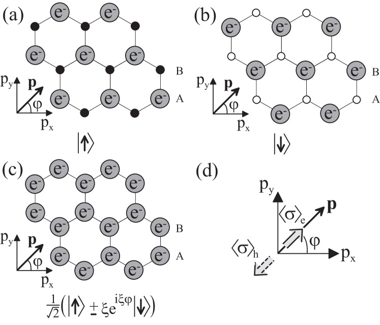
Figure 6: Schematic representation of the pseudospin degree of freedom: (a) electronic density solely on the $A$ sublattice can be viewed as a pseudospin ‘up’ state, whereas (b) density solely on the $B$ sublattice corresponds to a pseudospin ‘down’ state; (c) in graphene, electronic density is usually shared equally between $A$ and $B$ sublattices, so that the pseudospin part of the wave function is a linear combination of ‘up’ and ‘down,’ with amplitudes dependent on the direction of the electronic momentum $\mathbf{p}$; (d) at valley $K_{+}$, the pseudospin $\langle\mbox{\boldmath$\sigma$}\rangle_{e}$ in the conduction band is parallel to the momentum, whereas the pseudospin $\langle\mbox{\boldmath$\sigma$}\rangle_{h}$ in the valence band is anti-parallel to the momentum.

The effective Hamiltonian (80) and eigenstates (83) in the vicinity of the $K_{\xi}$ point have two components, reminiscent of the components of spin-$1/2$. Referring back to the original definitions of the components of the column vector $\psi$, (4) and (34), shows that this is not the physical spin of the electron, but a degree of freedom related to the relative amplitude of the Bloch function on the $A$ or $B$ sublattice. This degree of freedom is called pseudospin. If all the electronic density was located on the $A$ sublattice, Fig. 6(a), this could be viewed as a pseudospin ‘up’ state (pointing upwards out of the graphene sheet) $|\!\!\uparrow\rangle=(1,0)^{T}$, whereas density solely on the $B$ sublattice corresponds to a pseudospin ‘down’ state (pointing downwards out of the graphene sheet) $|\!\!\downarrow\rangle=(0,1)^{T}$, Fig. 6(b). In graphene, electronic density is usually shared equally between $A$ and $B$ sublattices, Fig. 6(c), so that the pseudospin part of the wave function is a linear combination of ‘up’ and ‘down,’ and it lies in the plane of the graphene sheet.

Not only do the electrons possess the pseudospin degree of freedom, but they are chiral, meaning that the orientation of the pseudospin is related to the direction of the electronic momentum $\mathbf{p}$. This is reflected in the fact that the amplitudes on the $A$ or $B$ sublattice of the eigenstate (83) depend on the polar angle $\varphi$. It is convenient to use Pauli spin matrices in the $A$/$B$ sublattice space, $\sigma_{i}$ where $i=1\ldots 3$, to write the effective Hamiltonian (80) as

$$H_{1,\xi}=v\left(\xi\sigma_{x}p_{x}+\sigma_{y}p_{y}\right)\,.$$ (84)

If we define a pseudospin vector as $\mbox{\boldmath$\sigma$}=\left(\sigma_{x},\sigma_{y},\sigma_{z}\right)$, and a unit vector as $\mathbf{\hat{n}}_{1}=\left(\xi\cos\varphi,\sin\varphi,0\right)$, then the Hamiltonian becomes $H_{1,\xi}=vp\,\mbox{\boldmath$\sigma$}.\mathbf{\hat{n}}_{1}$, stressing that the pseudospin $\sigma$ is linked to the direction $\mathbf{\hat{n}}_{1}$. The chiral operator $\mbox{\boldmath$\sigma$}.\mathbf{\hat{n}}_{1}$ projects the pseudospin onto the direction of quantization $\mathbf{\hat{n}}_{1}$: eigenstates of the Hamiltonian are also eigenstates of $\mbox{\boldmath$\sigma$}.\mathbf{\hat{n}}_{1}$ with eigenvalues $\pm 1$, $\mbox{\boldmath$\sigma$}.\mathbf{\hat{n}}_{1}\psi_{\pm}=\pm\psi_{\pm}$. An alternative way of expressing this chiral property of electrons is to explicitly calculate the expectation value of the pseudospin operator $\langle\mbox{\boldmath$\sigma$}\rangle=\left(\langle\sigma_{x}\rangle,\langle\sigma_{y}\rangle,\langle\sigma_{z}\rangle\right)$ with respect to the eigenstate $\psi_{\pm}$, (83). The result, $\langle\mbox{\boldmath$\sigma$}\rangle_{e/h}=\pm\left(\xi\cos\varphi,\sin\varphi,0\right)$, shows the link between pseudospin and momentum. For valley $K_{+}$, the pseudospin in the conduction band $\langle\mbox{\boldmath$\sigma$}\rangle_{e}$ is parallel to the momentum, whereas the pseudospin in the valence band $\langle\mbox{\boldmath$\sigma$}\rangle_{h}$ is anti-parallel to it, Fig. 6(d).

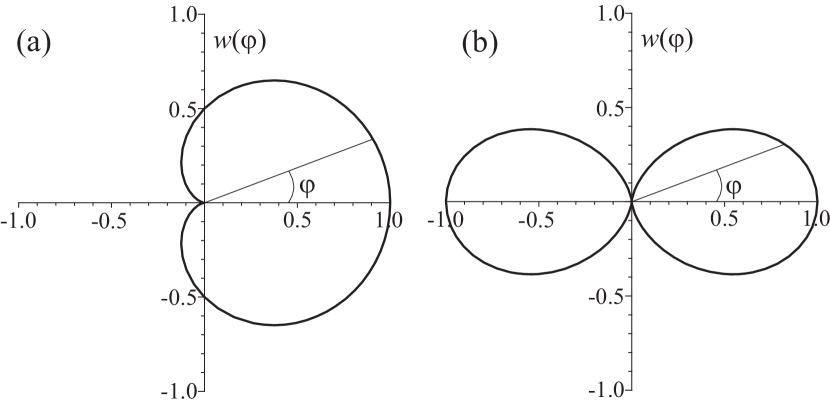
Figure 7: Anisotropic scattering of chiral electrons in graphene: (a) angular dependence $w(\varphi)=\cos^{2}(\varphi/2)$ of the scattering probability off an $A$-$B$ symmetric potential in monolayer graphene ando98 ; mceuen99 ; suz02 and (b) $w(\varphi)=\cos^{2}(\varphi)$ in bilayer graphene mcc06a ; falko07 .

If the electronic momentum $\mathbf{p}$ rotates by angle $\varphi$, then adiabatic evolution of the chiral wave function $\psi_{\pm}$, (83), produces a matching rotation of the vector $\mathbf{\hat{n}}_{1}$ by angle $\varphi$. For traversal of a closed contour in momentum space, corresponding to $\varphi=2\pi$, then the chiral wave function undergoes a phase change of $\pi$ known as Berry’s phase pan56 ; berry84 . It can be thought of as arising from the rotation of the pseudospin degree of freedom.

The chiral nature of low-energy electrons in graphene places an additional constraint on their scattering properties. If a given potential doesn’t break the $A$-$B$ symmetry, then it is unable to influence the pseudospin degree of freedom which must, therefore, be conserved upon scattering. Considering only the pseudospin part of the chiral wave function $\psi_{\pm}$, (83), the probability to scatter in a direction $\varphi$, where $\varphi=0$ is the forwards direction, is proportional to $w(\varphi)=|\langle\psi_{\pm}(\varphi)|\psi_{\pm}(0)\rangle|^{2}$. For monolayer graphene, $w(\varphi)=\cos^{2}(\varphi/2)$, Fig. 7(a). This is anisotropic, and displays an absence of backscattering $w(\pi)=0$ ando98 ; mceuen99 ; suz02 : scattering into a state with opposite momentum is prohibited because it requires a reversal of the pseudospin. Such conservation of pseudospin is at the heart of anisotropic scattering at potential barriers in graphene monolayers che06 ; kat06 , known as Klein tunneling.

0.6 The tight-binding model of bilayer graphene

In this section, we describe the tight-binding model of bilayer graphene. To do so, we use the tight-binding model described in Sect. 0.3 in order to generalize the model for monolayer graphene discussed in Sect. 0.4.

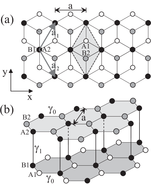
Figure 8: Schematic representation of the crystal structure of $AB$-stacked bilayer graphene: (a) plan view with $A1$ (white) and $B1$ atoms (black) on the lower layer, $A2$ (black) and $B2$ atoms (grey) on the upper layer. Vectors $\mathbf{a}_{1}$ and $\mathbf{a}_{2}$ are primitive lattice vectors of length equal to the lattice constant $a$, and the shaded rhombus is a unit cell; (b) side view where the parameter $\gamma_{0}$ represents nearest-neighbor coupling within each layer, $\gamma_{1}$ nearest-neighbor coupling between the $B1$ and $A2$ atoms on different layers.

We consider Bernal-stacked bilayer graphene trickey ; novo06 ; mcc06a (also called $AB$-stacked bilayer graphene). It consists of two parallel layers of carbon atoms, each arranged with a honeycomb arrangement as in a monolayer, that are coupled together, Fig. 6. There are four atoms in the unit cell, a pair $A1$, $B1$, from the lower layer and a pair $A2$, $B2$, from the upper layer. In Bernal stacking, the layers are arranged so that two atoms, $B1$ and $A2$, are directly below or above each other, whereas the other two atoms, $A1$ and $B2$, do not have a counterpart in the other layer. The primitive lattice vectors $\mathbf{a}_{1}$ and $\mathbf{a}_{2}$, and the lattice constant $a$ are the same as for monolayer graphene, and the unit cell, shown in Fig. 6(a), has the same area in the $x$-$y$ plane as in the monolayer. Therefore, the reciprocal lattice and first Brillouin zone are the same as in monolayer graphene, Fig. 2. The unit cell of bilayer graphene contains four atoms, and, if the tight-binding model includes one $p_{z}$ orbital per atomic site, there will be four bands near zero energy, instead of the two bands in monolayer graphene.

Essential features of the low-energy electronic band structure may be described by a minimal tight-binding model including nearest-neighbor coupling $\gamma_{0}$ between $A1$ and $B1$, and $A2$ and $B2$, atoms on each layer, and nearest-neighbor interlayer coupling $\gamma_{1}$ between $B1$ and $A2$ atoms that are directly below or above each other,

$$\gamma_{1}=\langle\phi_{A2}\left(\mathbf{r}-\mathbf{R}_{A2}\right)|{\cal H}|\phi_{B1}\left(\mathbf{r}-\mathbf{R}_{B1}\right)\rangle\,.$$ (85)

Then, we can generalize the treatment of monolayer graphene, (66), to write the transfer and overlap integral matrices of bilayer graphene, in a basis with components $A1$, $B1$, $A2$, $B2$, as

$$H = \left(\begin{array}[]{cccc}\epsilon_{2p}&-\gamma_{0}f\left(\mathbf{k}\right)&0&0\\ -\gamma_{0}f^{\ast}\left(\mathbf{k}\right)&\epsilon_{2p}&\gamma_{1}&0\\ 0&\gamma_{1}&\epsilon_{2p}&-\gamma_{0}f\left(\mathbf{k}\right)\\ 0&0&-\gamma_{0}f^{\ast}\left(\mathbf{k}\right)&\epsilon_{2p}\\ \end{array}\right)\,,$$ (90)

$$S = \left(\begin{array}[]{cccc}1&s_{0}f\left(\mathbf{k}\right)&0&0\\ s_{0}f^{\ast}\left(\mathbf{k}\right)&1&0&0\\ 0&0&1&s_{0}f\left(\mathbf{k}\right)\\ 0&0&s_{0}f^{\ast}\left(\mathbf{k}\right)&1\\ \end{array}\right)\,.$$ (95)

The upper-left and lower-right $2\times 2$ blocks describe behavior within the lower ($A1$/$B1$) and upper ($A2$/$B2$) layers, respectively. The off-diagonal $2\times 2$ blocks, containing parameter $\gamma_{1}$, describe interlayer coupling.

The band structure of bilayer graphene may be determined by solving the secular equation $\det\left(H-E_{j}S\right)=0$, (36). It is plotted in Fig. 9 for parameter values $\gamma_{0}=3.033$eV, $s_{0}=0.129$, $\epsilon_{2p}=0$ saito and interlayer coupling $\gamma_{1}=0.39$eV. There are four energy bands, two conduction bands and two valence bands. Overall, the band structure is similar to that of monolayer graphene, Fig. 5, with each monolayer band split into two by an energy approximately equal to the interlayer coupling $\gamma_{1}$ trickey . The most interesting part of the band structure is in the vicinity of the $K$ points mcc06a , as shown in the left inset of Fig. 9 which focuses in on the bands around $K_{-}$. At the $K$ point, one of the conduction (valence) bands is split away from zero energy by an amount equal to the interlayer coupling $\gamma_{1}$ (-$\gamma_{1}$). The split bands originate from atomic sites $B1$ and $A2$ that have a counterpart atom directly above or below them on the other layer. Orbitals on these pairs of atoms ($B1$ and $A2$) are strongly coupled by the interlayer coupling $\gamma_{1}$ and they form a bonding and anti-bonding pair of bands, split away from zero energy. In the following, we refer to them as ‘dimer’ states, and atomic sites $B1$ and $A2$ are called ‘dimer’ sites. The remaining two bands, one conduction and one valence band, touch at zero energy: as in the monolayer, there is no band gap between the conduction and valence bands. In the vicinity of the $K$ points, the dispersion of the latter bands is quadratic $E_{\pm}\propto\pm|\mathbf{k}-\mathbf{K}_{\xi}|^{2}$, and electronic properties of the low-energy bands may be described by an effective Hamiltonian describing massive chiral particles. This will be explored in more detail in the next section.

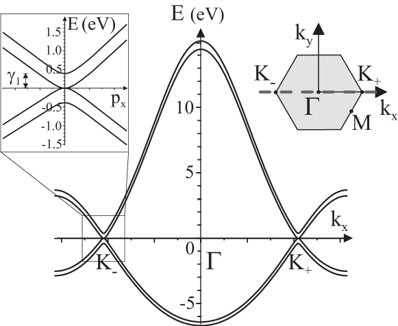
Figure 9: The low-energy band structure of bilayer graphene taking into account nearest-neighbor hopping with parameter $\gamma_{0}=3.033$eV, nearest-neighbor overlap parameter $s_{0}=0.129$, orbital energy $\epsilon_{2p}=0$ saito , and interlayer coupling $\gamma_{1}=0.39$eV. The plot shows the bands calculated along the $k_{x}$ axis intersecting points $K_{-}$, $\Gamma$, and $K_{+}$ in the Brillouin zone, shown as the dotted line in the right inset. The left inset shows the band structure in the vicinity of the point $K_{-}$.

0.7 Massive chiral quasiparticles in bilayer graphene

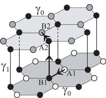
Figure 10: Schematic representation of the crystal structure of $AB$-stacked bilayer graphene illustrating the processes that contribute to effective coupling between $A1$ (white) and $B2$ atoms (grey), in the presence of strongly-coupled ‘dimer’ sites $B1$ and $A2$ (black). The black arrowed line indicates the three stage process: intralayer hopping between $A1$ and $B1$, followed by an interlayer transition via the dimer sites $B1$ and $A2$, followed by another intralayer hopping between $A2$ and $B2$.

0.7.1 The low-energy bands of bilayer graphene

To begin the description of the low-energy bands in bilayer graphene, we set $s_{0}=0$, thus neglecting the non-orthogonality of orbitals that tends to become important at high energy. Then, the overlap matrix $S$, (95), becomes a unit matrix, and $H$, (90), is an effective Hamiltonian for the four bands of bilayer graphene at low-energy mcc06a :

$$H=\left(\begin{array}[]{cccc}0&-\gamma_{0}f\left(\mathbf{k}\right)&0&0\\ -\gamma_{0}f^{\ast}\left(\mathbf{k}\right)&0&\gamma_{1}&0\\ 0&\gamma_{1}&0&-\gamma_{0}f\left(\mathbf{k}\right)\\ 0&0&-\gamma_{0}f^{\ast}\left(\mathbf{k}\right)&0\\ \end{array}\right)\,,$$ (100)

where we used $\epsilon_{2p}=0$ saito to define the zero of the energy axis to coincide with the energy of the $2p_{z}$ orbital. Eigenvalues of the Hamiltonian are given by

$$E_{\pm}^{(\alpha)}=\pm\frac{\gamma_{1}}{2}\left(\sqrt{1+\frac{4\gamma_{0}^{2}|f(\mathbf{k})|^{2}}{\gamma_{1}^{2}}}+\alpha\right)\,,\qquad\alpha=\pm 1\,.$$ (101)

Over most of the Brillouin zone, where $4\gamma_{0}^{2}|f(\mathbf{k})|^{2}\gg\gamma_{1}^{2}$, the energy may be approximated as $E_{\pm}^{(\alpha)}\approx\pm(\gamma_{0}|f(\mathbf{k})|+\alpha\gamma_{1}/2)$, meaning that the $\alpha=\pm 1$ bands are approximately the same as the monolayer bands, (71), but they are split by the interlayer coupling $\gamma_{1}$. The eigenvalues $E_{\pm}^{(1)}$, (101), describe two bands that are split away from zero energy by $\pm\gamma_{1}$ at the $K$ point (where $|f(\mathbf{k})|=0$) as shown in the left inset of Fig. 9. This is because the orbitals on the $A2$ and $B1$ sites form a dimer that is coupled by interlayer hopping $\gamma_{1}$, resulting in a bonding and anti-bonding pair of states $\pm\gamma_{1}$.

The remaining two bands are described by $E_{\pm}^{(-1)}$. Near to the $K_{\xi}$ point, $pa/\hbar\ll 1$, we replace the factor $\gamma_{0}|f(\mathbf{k})|$ with $vp$, (77):

$$E_{\pm}^{(-1)}\approx\pm\frac{\gamma_{1}}{2}\left(\sqrt{1+\frac{4v^{2}p^{2}}{\gamma_{1}^{2}}}-1\right)\,.$$ (102)

This formula interpolates between linear dispersion at large momenta ($\gamma_{1}\ll vp<\gamma_{0}$) and quadratic dispersion $E_{\pm}^{(-1)}\approx\pm v^{2}p^{2}/\gamma_{1}$ near zero energy where the bands touch. These bands arise from effective coupling between the orbitals on sites, $A1$ and $B2$, that don’t have a counterpart in the other layer. In the absence of direct coupling between $A1$ and $B2$, the effective coupling is achieved through a three stage process as indicated in Fig. 10. It can be viewed as an intralayer hopping between $A1$ and $B1$, followed by an interlayer transition via the dimer sites $B1$ and $A2$, followed by another intralayer hopping between $A2$ and $B2$. This effective coupling may be succinctly described by an effective low-energy Hamiltonian written in a two-component basis of $p_{z}$ orbitals on $A1$ and $B2$ sites.

0.7.2 The two-component Hamiltonian of bilayer graphene

The effective two-component Hamiltonian may be derived from the four component Hamiltonian, (100), using a Schrieffer-Wolff transformation swtrans ; mcc06a . In the present context, a straightforward way to do the transformation is to consider the eigenvalue equation for the four component Hamiltonian, (100), as four simultaneous equations for the wave-function components ${c}_{A1}$, ${c}_{B1}$, ${c}_{A2}$, ${c}_{B2}$:

$$E{c}_{A1}+\gamma_{0}f\left(\mathbf{k}\right){c}_{B1} = 0\,,$$ (103)

$$\gamma_{0}f^{\ast}\left(\mathbf{k}\right){c}_{A1}+E{c}_{B1}-\gamma_{1}{c}_{A2} = 0\,,$$ (104)

$$-\gamma_{1}{c}_{B1}+E{c}_{A2}+\gamma_{0}f\left(\mathbf{k}\right){c}_{B2} = 0\,,$$ (105)

$$\gamma_{0}f^{\ast}\left(\mathbf{k}\right){c}_{A2}+E{c}_{B2} = 0\,.$$ (106)

Using the second and third equations, (104) and (105), it is possible to express the components on the dimer sites, ${c}_{B1}$ and ${c}_{A2}$, in terms of the other two:

$${c}_{B1} = \frac{\gamma_{0}f\left(\mathbf{k}\right)}{\gamma_{1}d}{c}_{B2}+\frac{E\gamma_{0}f^{\ast}\left(\mathbf{k}\right)}{\gamma_{1}^{2}d}{c}_{A1},$$ (107)

$${c}_{A2} = \frac{E\gamma_{0}f\left(\mathbf{k}\right)}{\gamma_{1}^{2}d}{c}_{B2}+\frac{\gamma_{0}f^{\ast}\left(\mathbf{k}\right)}{\gamma_{1}d}{c}_{A1}\,,$$ (108)

where $d=1-E^{2}/\gamma_{1}^{2}$. Substituting these expressions into the first and fourth equations, (103) and (106), produces two equations solely in terms of ${c}_{A1}$ and ${c}_{B2}$. Assuming $|E|\ll|\gamma_{1}|$ and $|\gamma_{0}f\left(\mathbf{k}\right)|\ll|\gamma_{1}|$, we use $d\approx 1$ and keep terms up to order $1/\gamma_{1}$ only:

$$E{c}_{A1}+\frac{\gamma_{0}^{2}f^{2}\left(\mathbf{k}\right)}{\gamma_{1}}{c}_{B2} = 0\,,$$ (109)

$$\frac{\gamma_{0}^{2}(f^{\ast}\left(\mathbf{k}\right))^{2}}{\gamma_{1}}{c}_{A1}+E{c}_{B2} = 0\,.$$ (110)

It is possible to express these two equations as a Schrödinger equation, $H_{2}\psi=E\psi$, with a two-component wave function $\psi=\left({c}_{A1},{c}_{B2}\right)^{T}$ and two-component Hamiltonian

$$H_{2,\xi}=-\frac{1}{2m}\left(\begin{array}[]{cc}0&\left(\xi p_{x}-ip_{y}\right)^{2}\\ \left(\xi p_{x}+ip_{y}\right)^{2}&0\\ \end{array}\right)\,,$$ (113)

where we used the approximation $f\left(\mathbf{k}\right)\approx-v\left(\xi p_{x}-ip_{y}\right)/\gamma_{0}$, (77), valid for momentum $pa/\hbar\ll 1$ close to the $K_{\xi}$ point, and parameters $v$ and $\gamma_{1}$ were combined into a mass $m=\gamma_{1}/(2v^{2})$.

The effective low-energy Hamiltonian of bilayer graphene, (113), resembles the Dirac-like Hamiltonian of monolayer graphene, (80), but with a quadratic term on the off-diagonal instead of linear. The energy eigenvalues and eigenstates of $H_{2}$ are given by

$$E_{\pm}=\pm\frac{p^{2}}{2m}\,,\qquad\psi_{\pm}=\frac{1}{\sqrt{2}}\left(\begin{array}[]{c}1\\ \mp e^{i2\xi\varphi}\\ \end{array}\right)e^{i\mathbf{p}.\mathbf{r}/\hbar}\,,$$ (116)

where $\pm$ refer to the conduction and valence bands, respectively. Here $\varphi$ is the polar angle of the momentum in the graphene plane, $\mathbf{p}=\left(p_{x},p_{y}\right)=p\left(\cos\varphi,\sin\varphi\right)$.

0.7.3 Pseudospin and chirality in bilayer graphene

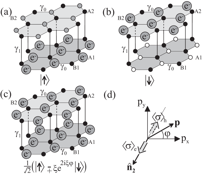
Figure 11: Schematic representation of the pseudospin degree of freedom in bilayer graphene: (a) electronic density solely on the $A1$ sublattice on the lower layer can be viewed as a pseudospin ‘up’ state, whereas (b) density solely on the $B2$ sublattice on the upper layer corresponds to a pseudospin ‘down’ state; (c) in bilayer graphene, electronic density is usually shared equally between $A1$ and $B2$ sublattices, so that the pseudospin part of the wave function is a linear combination of ‘up’ and ‘down,’ with amplitudes dependent on the direction of the electronic momentum $\mathbf{p}$; (d) at valley $K_{+}$, the pseudospin $\langle\mbox{\boldmath$\sigma$}\rangle_{e}$ in the conduction band is parallel to the quantization direction $\mathbf{\hat{n}}_{2}$, whereas the pseudospin $\langle\mbox{\boldmath$\sigma$}\rangle_{h}$ in the valence band is anti-parallel to $\mathbf{\hat{n}}_{2}$. Direction $\mathbf{\hat{n}}_{2}$ is related to the direction of momentum $\mathbf{p}$, but turns in the $x$-$y$ plane twice as quickly as it.

The two-component Hamiltonian (113) of bilayer graphene has a pseudospin degree of freedom novo06 ; mcc06a related to the amplitude of the eigenstates (116) on the $A1$ and $B2$ sublattice sites, where $A1$ and $B2$ lie on different layers. If all the electronic density was located on the $A1$ sublattice, Fig. 11(a), this could be viewed as a pseudospin ‘up’ state (pointing upwards out of the graphene sheet) $|\!\!\uparrow\rangle=(1,0)^{T}$, whereas density solely on the $B2$ sublattice corresponds to a pseudospin ‘down’ state (pointing downwards out of the graphene sheet) $|\!\!\downarrow\rangle=(0,1)^{T}$, Fig. 11(b). In bilayer graphene, electronic density is usually shared equally between the two sublattices, Fig. 11(c), so that the pseudospin part of the wave function is a linear combination of ‘up’ and ‘down,’ and it lies in the plane of the graphene sheet.

Electrons in bilayer graphene are chiral novo06 ; mcc06a , meaning that the orientation of the pseudospin is related to the direction of the electronic momentum $\mathbf{p}$, but the chirality is different to that in monolayers. As before, we use Pauli spin matrices in the $A1$/$B2$ sublattice space, $\sigma_{i}$ where $i=1\ldots 3$, to write the effective Hamiltonian (113) as

$$H_{2,\xi}=-\frac{1}{2m}\left[\sigma_{x}\left(p_{x}^{2}-p_{y}^{2}\right)+2\xi\sigma_{y}p_{x}p_{y}\right]\,.$$ (117)

If we define a pseudospin vector as $\mbox{\boldmath$\sigma$}=\left(\sigma_{x},\sigma_{y},\sigma_{z}\right)$, and a unit vector as $\mathbf{\hat{n}}_{2}=-\left(\cos 2\varphi,\xi\sin 2\varphi,0\right)$, then the Hamiltonian becomes $H_{2,\xi}=(p^{2}/2m)\,\mbox{\boldmath$\sigma$}.\mathbf{\hat{n}}_{2}$, stressing that the pseudospin $\sigma$ is linked to the direction $\mathbf{\hat{n}}_{2}$. The chiral operator $\mbox{\boldmath$\sigma$}.\mathbf{\hat{n}}_{2}$ projects the pseudospin onto the direction of quantization $\mathbf{\hat{n}}_{2}$: eigenstates of the Hamiltonian are also eigenstates of $\mbox{\boldmath$\sigma$}.\mathbf{\hat{n}}_{2}$ with eigenvalues $\pm 1$, $\mbox{\boldmath$\sigma$}.\mathbf{\hat{n}}_{2}\psi_{\pm}=\pm\psi_{\pm}$. In bilayer graphene, the quantization axis $\mathbf{\hat{n}}_{2}$ is fixed to lie in the graphene plane, but it turns twice as quickly in the plane as the momentum $\mathbf{p}$. If we calculate the expectation value of the pseudospin operator $\langle\mbox{\boldmath$\sigma$}\rangle=\left(\langle\sigma_{x}\rangle,\langle\sigma_{y}\rangle,\langle\sigma_{z}\rangle\right)$ with respect to the eigenstate $\psi_{\pm}$, (116), then the result $\langle\mbox{\boldmath$\sigma$}\rangle_{e/h}=\mp\left(\cos 2\varphi,\xi\sin 2\varphi,0\right)$, illustrates the link between pseudospin and momentum, Fig. 11(d).

If the momentum $\mathbf{p}$ rotates by angle $\varphi$, adiabatic evolution of the chiral wave function $\psi_{\pm}$, (116), produces a matching rotation of the quantization axis $\mathbf{\hat{n}}_{2}$ by angle $2\varphi$, not $\varphi$ as in the monolayer, Sect. 0.5.2. Thus, traversal around a closed contour in momentum space results in a Berry’s phase pan56 ; berry84 change of $2\pi$ of the chiral wave function in bilayer graphene novo06 ; mcc06a . For Berry’s phase $2\pi$ chiral electrons in bilayer graphene, (116), the probability to scatter in a direction $\varphi$, where $\varphi=0$ is the forwards direction, is proportional to $w(\varphi)=|\langle\psi_{\pm}(\varphi)|\psi_{\pm}(0)\rangle|^{2}=\cos^{2}(\varphi)$ mcc06a ; falko07 as shown in Fig. 7(b). This is anisotropic, but, unlike monolayers Fig. 7(a), does not display an absence of backscattering ($w(\pi)=1$ in bilayers): scattering into a state with opposite momentum is not prohibited because it doesn’t require a reversal of the pseudospin.

0.8 The integer quantum Hall effect in graphene

When a perpendicular magnetic field is applied a two-dimensional electron gas, the electrons follow cyclotron orbits, and their allowed energies are quantized into values known as Landau levels landau . At low magnetic field, the Landau levels give rise to quantum oscillations including the de Haas-van Alphen effect and the Shubnikov-de Haas effect. At higher fields, the discrete Landau level spectrum is manifest in the integer quantum Hall effect vk80 ; p+r87 ; macdonald89 , a quantization of Hall conductivity into integer values of the quantum of conductivity $e^{2}/h$. For monolayer graphene, the Landau level spectrum was calculated over fifty years ago by McClure mcclure56 , and the integer quantum Hall effect was observed novo05 ; zhang05 and studied theoretically haldane88 ; zheng02 ; gusynin05 ; peres06 ; herbut07 in recent years. The chiral nature of electrons in graphene results in an unusual sequencing of the quantized plateaus of the Hall conductivity. In bilayer graphene, the experimental observation of the integer quantum Hall effect novo06 and calculation of the Landau level spectrum mcc06a revealed further unusual features related to the chirality of electrons.

0.8.1 The Landau level spectrum of monolayer graphene

We consider a magnetic field perpendicular to the graphene sheet $\mathbf{B}=\left(0,0,-B\right)$ where $B=|\mathbf{B}|$. The Dirac-like Hamiltonian of monolayer graphene (80) may be written as

$$\!\!\!\!\!\!H_{1,K_{+}}=v\left(\begin{array}[]{cc}0&\pi^{\dagger}\\ \pi&0\\ \end{array}\right),\quad H_{1,K_{-}}=-v\left(\begin{array}[]{cc}0&\pi\\ \pi^{\dagger}&0\\ \end{array}\right),\quad\Big{\{}\begin{array}[]{c}\pi=p_{x}+ip_{y}\\ \pi^{\dagger}=p_{x}-ip_{y}\end{array},$$ (124)

in the vicinity of corners of the Brillouin zone $K_{+}$ and $K_{-}$, respectively. The off-diagonal elements of the Hamiltonian (124) contain operators $\pi=p_{x}+ip_{y}$ and $\pi^{\dagger}=p_{x}-ip_{y}$, where, in the presence of a magnetic field, the operator $\mathbf{p}=(p_{x},p_{y})\equiv-i\hbar\nabla+e\mathbf{A}$. Here $\mathbf{A}$ is the vector potential and the charge of the electron is $-e$.

Using the Landau gauge $\mathbf{A}=\left(0,-Bx,0\right)$ preserves translational invariance in the $y$ direction, so that eigenstates may be written in terms of states that are plane waves in the $y$ direction and harmonic oscillator states in the $x$ direction p+r87 ; macdonald89 ,

$$\phi_{\ell}\left(x,y\right)=A_{\ell}{\cal H}_{\ell}\!\!\left(\frac{x}{\lambda_{B}}-\frac{p_{y}\lambda_{B}}{\hbar}\right)\!\exp\!\!\left[-\frac{1}{2}\left(\frac{x}{\lambda_{B}}-\frac{p_{y}\lambda_{B}}{\hbar}\right)^{2}+i\frac{p_{y}y}{\hbar}\right]\!\!.$$ (125)

Here, ${\cal H}_{\ell}$ are Hermite polynomials of order ${\ell}$, for integer ${\ell}\geq 0$, and the normalization constant is $A_{\ell}=1/\sqrt{2^{\ell}{\ell}!\sqrt{\pi}}$. The magnetic length $\lambda_{B}$, and a related energy scale $\Gamma$, are defined as

$$\lambda_{B}=\sqrt{\frac{\hbar}{eB}}\,,\qquad\Gamma=\frac{\sqrt{2}\hbar v}{\lambda_{B}}=\sqrt{2\hbar v^{2}eB}\,.$$ (126)

With this choice of vector potential, $\pi=-i\hbar\partial_{x}+\hbar\partial_{y}-ieBx$ and $\pi^{\dagger}=-i\hbar\partial_{x}-\hbar\partial_{y}+ieBx$. Acting on the harmonic oscillator states (125) gives

$$\pi\phi_{\ell} = -\frac{\sqrt{2}i\hbar}{\lambda_{B}}\sqrt{{\ell}}\,\phi_{{\ell}-1}\,,$$ (127)

$$\pi^{\dagger}\phi_{\ell} = \frac{\sqrt{2}i\hbar}{\lambda_{B}}\sqrt{{\ell}+1}\,\phi_{{\ell}+1}\,,$$ (128)

and $\pi\phi_{0}=0$. These equations indicate that operators $\pi$ and $\pi^{\dagger}$ are proportional to lowering and raising operators of the harmonic oscillator states $\phi_{\ell}$. The Landau level spectrum is, therefore, straightforward to calculate mcclure56 ; fisch70 ; zheng02 . At the first valley, $K_{+}$, the Landau level energies and eigenstates of $H_{1,K_{+}}$ are

$$K_{+},\,{\ell}\geq 1:\quad E_{{\ell},\pm} = \pm\frac{\sqrt{2}\hbar v}{\lambda_{B}}\sqrt{{\ell}}\,,\qquad\psi_{{\ell},\pm}=\frac{1}{\sqrt{2}}\left(\begin{array}[]{c}\phi_{\ell}\\ \mp i\phi_{{\ell}-1}\\ \end{array}\right),$$ (131)

$$K_{+},\,{\ell}=0:\quad\,\,\,\,\,E_{0} = 0\,,\qquad\qquad\qquad\,\,\psi_{0}=\left(\begin{array}[]{c}\phi_{0}\\ 0\\ \end{array}\right),$$ (134)

where $\pm$ refer to the conduction and valence bands, respectively. Equation (131) describes an electron (plus sign) and a hole (minus sign) series of energy levels, with prefactor $\Gamma=\sqrt{2}\hbar v/\lambda_{B}$ (126), proportional to the square root of the magnetic field. In addition, there is a special level (134) fixed at zero energy that arises from the presence of the lowering operator in the Hamiltonian, $\pi\phi_{0}=0$. The corresponding eigenfunction $\psi_{0}$ has non-zero amplitude on the $A$ sublattice, but its amplitude is zero on the $B$ sublattice. The form (124) of the Hamiltonian $H_{1,K_{-}}$ at the second valley, $K_{-}$, shows that its spectrum is degenerate with that at $K_{+}$, with the role of the $A$ and $B$ sublattices reversed:

$$K_{-},\,{\ell}\geq 1:\quad E_{{\ell},\pm} = \pm\frac{\sqrt{2}\hbar v}{\lambda_{B}}\sqrt{{\ell}}\,,\qquad\psi_{{\ell},\pm}=\frac{1}{\sqrt{2}}\left(\begin{array}[]{c}\pm i\phi_{{\ell}-1}\\ \phi_{\ell}\\ \end{array}\right),$$ (137)

$$K_{-},\,{\ell}=0:\quad\,\,\,\,\,E_{0} = 0\,,\qquad\qquad\qquad\,\,\psi_{0}=\left(\begin{array}[]{c}0\\ \phi_{0}\\ \end{array}\right).$$ (140)

Thus, the eigenfunction $\psi_{0}$ of the zero-energy level has zero amplitude on the $B$ sublattice at valley $K_{+}$ and zero amplitude on the $A$ sublattice at $K_{-}$. If we take into account electronic spin, which contributes a twofold degeneracy of the energy levels, as well as valley degeneracy, then the Landau level spectrum of monolayer graphene consists of fourfold-degenerate Landau levels.

0.8.2 The integer quantum Hall effect in monolayer graphene

In this section, we describe how the Landau level spectrum of graphene is reflected in the dependence of the Hall conductivity $\sigma_{xy}(n)$ on carrier density $n$. In conventional two-dimensional semiconductor systems, in the absence of any Berry’s phase effects, the Landau level spectrum is given by $E_{\ell}=\hbar\omega_{c}({\ell}+1/2)$, $\ell\geq 0$, where $\omega_{c}=eB/m$ is the cyclotron frequency p+r87 ; macdonald89 . Here, the lowest state lies at finite energy $E_{0}=\hbar\omega_{c}/2$. If the system has an additional degeneracy $g$ (for example, $g=2$ for spin), then plateaus vk80 ; p+r87 ; macdonald89 occur at quantized $\sigma_{xy}$ values of $N(ge^{2}/h)$ where $N$ is an integer and $e^{2}/h$ is the quantum value of conductance, i.e. each step between adjacent plateaus has height $ge^{2}/h$, Fig. 12(a). Each $\sigma_{xy}$ step coincides with the crossing of a Landau level on the density axis. Since the maximum carrier density per Landau level is $gB/\varphi_{0}$, where $\varphi_{0}=h/e$ is the flux quantum, the distance between the $\sigma_{xy}$ steps on the density axis is $gB/\varphi_{0}$.

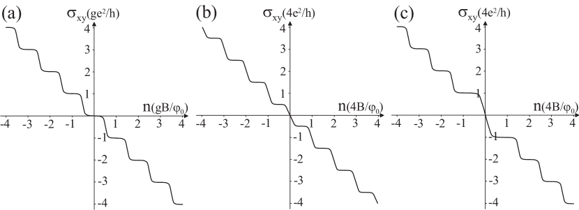
Figure 12: Schematic representation of three types of integer quantum Hall effect, showing the density dependence of the Hall conductivity $\sigma_{xy}(n)$: (a) conventional two-dimensional semiconductor systems with additional system degeneracy $g$; (b) monolayer graphene; (c) bilayer graphene. Here, $B$ is the magnitude of the magnetic field and $\varphi_{0}=h/e$ is the flux quantum.

As described above, monolayer graphene has fourfold (spin and valley) degenerate Landau levels $E_{{\ell},\pm}=\pm\sqrt{2{\ell}}\hbar v/\lambda_{B}$ for ${\ell}\geq 1$ and $E_{0}=0$. The Hall conductivity $\sigma_{xy}(n)$, Fig. 12(b), displays a series of quantized plateaus separated by steps of size $4e^{2}/h$, as in the conventional case, but the plateaus occur at half-integer values of $4e^{2}/h$ rather than integer ones:

$$\sigma_{xy}=-\frac{1}{2}\left(2N+1\right)\left(\frac{4e^{2}}{h}\right)\,,$$ (141)

where $N$ is an integer, as observed experimentally novo05 ; zhang05 and described theoretically haldane88 ; zheng02 ; gusynin05 ; peres06 ; herbut07 . This unusual sequencing of $\sigma_{xy}$ plateaus is explained by the presence of the fourfold-degenerate Landau level $E_{0}$ fixed at zero energy. Since it lies at the boundary between the electron and hole gases, it creates a step in $\sigma_{xy}$ of $4e^{2}/h$ at zero density. Each Landau level in monolayer graphene is fourfold degenerate, including the zero energy one, so the distance between each $\sigma_{xy}$ step on the density axis is $4B/\varphi_{0}$, i.e. the steps occur at densities equal to integer values of $4B/\varphi_{0}$.

0.8.3 The Landau level spectrum of bilayer graphene

In the presence of a perpendicular magnetic field, the Hamiltonian (113) describing massive chiral electrons in bilayer graphene may be written as

$$\!\!\!\!\!\!H_{2,K_{+}}=-\frac{1}{2m}\left(\begin{array}[]{cc}0&\left(\pi^{\dagger}\right)^{2}\\ \pi^{2}&0\\ \end{array}\right),\qquad H_{2,K_{-}}=-\frac{1}{2m}\left(\begin{array}[]{cc}0&\pi^{2}\\ \left(\pi^{\dagger}\right)^{2}&0\\ \end{array}\right),$$ (146)

in the vicinity of corners of the Brillouin zone $K_{+}$ and $K_{-}$, respectively. Using the action of operators $\pi$ and $\pi^{\dagger}$ on the harmonic oscillator states $\phi_{\ell}$, (127) and (128), the Landau level spectrum of bilayer graphene may be calculated mcc06a . At the first valley, $K_{+}$, the Landau level energies and eigenstates of $H_{2,K_{+}}$ are

$$\!\!\!K_{+},\,{\ell}\geq 2:\quad E_{{\ell},\pm} = \pm\frac{\hbar^{2}}{m\lambda_{B}^{2}}\sqrt{{\ell}({\ell}-1)}\,,\quad\psi_{{\ell},\pm}=\frac{1}{\sqrt{2}}\left(\begin{array}[]{c}\phi_{\ell}\\ \pm\phi_{{\ell}-2}\\ \end{array}\right)\!,$$ (149)

$$\!\!\!K_{+},\,{\ell}=1:\quad\,\,\,\,\,E_{1} = 0\,,\quad\qquad\qquad\qquad\qquad\psi_{1}=\left(\begin{array}[]{c}\phi_{1}\\ 0\\ \end{array}\right),$$ (152)

$$\!\!\!K_{+},\,{\ell}=0:\quad\,\,\,\,\,E_{0} = 0\,,\quad\qquad\qquad\qquad\qquad\psi_{0}=\left(\begin{array}[]{c}\phi_{0}\\ 0\\ \end{array}\right),$$ (155)

where $\pm$ refer to the conduction and valence bands, respectively. Equation (149) describes an electron (plus sign) and a hole (minus sign) series of energy levels. The prefactor $\hbar^{2}/(m\lambda_{B}^{2})$ is proportional to the magnetic field, and it may equivalently be written as $\Gamma^{2}/\gamma_{1}$ or as $\hbar\omega_{c}$ where $\omega_{c}=eB/m$. For high levels, ${\ell}\gg 1$, the spectrum consists of approximately equidistant levels with spacing $\hbar\omega_{c}$. Note, however, that we are considering the low-energy Hamiltonian, so that the above spectrum is only valid for sufficiently small level index and magnetic field $\sqrt{{\ell}}\Gamma\ll\gamma_{1}$. As well as the field-dependent levels, there are two special levels, (152) and (155), fixed at zero energy. There are two zero-energy levels because of the presence of the square of the lowering operator in the Hamiltonian. It may act on the oscillator ground state to give zero energy, $\pi^{2}\phi_{0}=0$, (155), but also on the first excited state to give zero energy, $\pi^{2}\phi_{1}=0$, (152). The corresponding eigenfunctions $\psi_{0}$ and $\psi_{1}$ have non-zero amplitude on the $A1$ sublattice, that lies on the bottom layer, but their amplitude is zero on the $B2$ sublattice.

The form (146) of the Hamiltonian $H_{2,K_{-}}$ at the second valley, $K_{-}$, shows that its spectrum is degenerate with that at $K_{+}$ with the role of the $A1$ and $B2$ sublattices reversed. It may be expressed as $H_{2,K_{-}}=\sigma_{x}H_{2,K_{+}}\sigma_{x}$ so that $\psi_{{\ell},\pm}(K_{-})=\sigma_{x}\psi_{{\ell},\pm}(K_{+})$, $\psi_{1}(K_{-})=\sigma_{x}\psi_{1}(K_{+})$, and $\psi_{0}(K_{-})=\sigma_{x}\psi_{0}(K_{+})$. Thus, the eigenfunctions $\psi_{0}$ and $\psi_{1}$ of the zero-energy levels have zero amplitude on the $B2$ sublattice at valley $K_{+}$ and zero amplitude on the $A1$ sublattice at $K_{-}$. If we take into account electronic spin, which contributes a twofold degeneracy of the energy levels, as well as valley degeneracy, then the Landau level spectrum of bilayer graphene consists of fourfold degenerate Landau levels, except for the zero-energy levels which are eightfold degenerate. This doubling of the degeneracy of the zero-energy levels is reflected in the density dependence of the Hall conductivity.

0.8.4 The integer quantum Hall effect in bilayer graphene

The Hall conductivity $\sigma_{xy}(n)$ of bilayer graphene, Fig. 12(c), displays a series of quantized plateaus occurring at integer values of $4e^{2}/h$ that is practically the same as in the conventional case, Fig. 12(a), with degeneracy per level $g=4$ accounting for spin and valleys. However, there is a step of size $8e^{2}/h$ in $\sigma_{xy}$ across zero density in bilayer graphene novo06 ; mcc06a . This unusual behavior is explained by the eightfold degeneracy of the zero-energy Landau levels. Their presence creates a step in $\sigma_{xy}$ at zero density, as in monolayer graphene, but owing to the doubled degeneracy as compared to other levels, it requires twice as many carriers to fill them. Thus, the transition between the corresponding plateaus is twice as wide in density, $8B/\varphi_{0}$ as compared to $4B/\varphi_{0}$, and the step in $\sigma_{xy}$ between the plateaus must be twice as high, $8e^{2}/h$ instead of $4e^{2}/h$. This demonstrates that, although Berry’s phase $2\pi$ is not reflected in the sequencing of quantum Hall plateaus at high density, it has a consequence in the quantum limit of zero density, as observed experimentally novo06 .

Here, we showed that the chiral Hamiltonians of monolayer and bilayer graphene corresponding to Berry’s phase $\pi$ and $2\pi$, respectively, have associated four- and eight-fold degenerate zero-energy Landau levels, producing steps of four and eight times the conductance quantum $e^{2}/h$ in the Hall conductivity across zero density novo05 ; zhang05 ; novo06 . In our discussion, we neglected interaction effects and we assumed that any valley and spin splitting, or splitting of the ${\ell}=1$ and ${\ell}=0$ levels in bilayer graphene, are negligible as compared to temperature and level broadening.

0.9 Trigonal warping in graphene

So far, we have described the tight-binding model of graphene and showed that the low-energy Hamiltonians of monolayer and bilayer graphene support chiral electrons with unusual properties. There are, however, additional contributions to the Hamiltonians that perturb this simple picture. In this section, we focus on one of them, known in the graphite literature as trigonal warping dre74 ; nak76 ; ino62 ; gup72 ; dressel02 .

0.9.1 Trigonal warping in monolayer graphene

The band structure of monolayer graphene, shown in Fig. 4, is approximately linear in the vicinity of zero energy, but it shows deviations away from linear behavior at higher energy. In deriving the Dirac-like Hamiltonian of monolayer graphene (80), we kept only linear terms in the momentum $\mathbf{p}=\hbar\mathbf{k}-\hbar\mathbf{K}_{\xi}$ measured with respect to the $K_{\xi}$ point. If we retain quadratic terms in $\mathbf{p}$, then the function $f(\mathbf{k})$, (77), describing coupling between the $A$ and $B$ sublattices becomes

$$f\left(\mathbf{k}\right) \approx -\frac{\sqrt{3}a}{2\hbar}(\xi p_{x}-ip_{y})+\frac{a^{2}}{8\hbar^{2}}(\xi p_{x}+ip_{y})^{2},$$ (156)

where $pa/\hbar\ll 1$. Using this approximate expression, the Dirac-like Hamiltonian (80) in the vicinity of point $K_{\xi}$ is modified ando98 as

$$\!\!\!H_{1,\xi}=v\left(\begin{array}[]{cc}0&\xi p_{x}-ip_{y}\\ \xi p_{x}+ip_{y}&0\\ \end{array}\right)-\mu\left(\begin{array}[]{cc}0&\left(\xi p_{x}+ip_{y}\right)^{2}\\ \left(\xi p_{x}-ip_{y}\right)^{2}&0\\ \end{array}\right)\!,$$ (161)

where parameter $\mu=\gamma_{0}a^{2}/(8\hbar^{2})$. The corresponding energy eigenvalues are

$$E_{\pm}=\pm\sqrt{v^{2}p^{2}-2\xi\mu vp^{3}\cos 3\varphi+\mu^{2}p^{4}}\,,$$ (162)

For small momentum near the $K$ point, $pa/\hbar\ll 1$, the terms containing parameter $\mu$ are a small perturbation because $\mu p^{2}/(vp)=pa/(4\sqrt{3}\hbar)$. They contribute to a weak triangular deformation of the Fermi circle that becomes stronger as the momentum $\mathbf{p}$ becomes larger. Figure 13 shows the trigonal warping of the Fermi circle near point $K_{+}$, obtained by plotting (162) for constant energy $E=0.5\gamma_{0}$. The presence of the valley index $\xi=\pm 1$ in the angular term of (162) means that the orientation of the trigonal warping at the second valley $K_{-}$ is reversed.

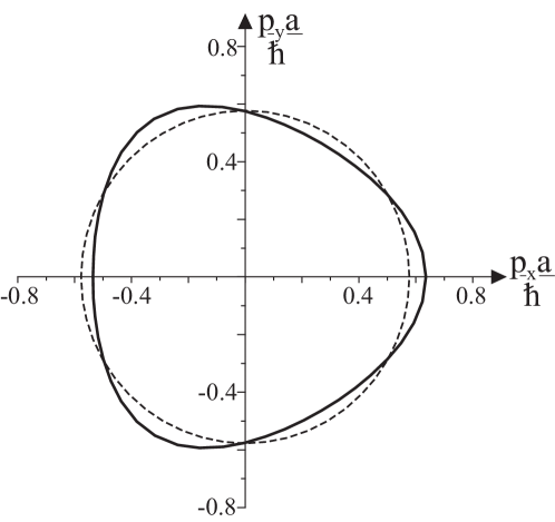
Figure 13: Trigonal warping in monolayer graphene. The solid line shows the isoenergetic line $E=0.5\gamma_{0}$ in the vicinity of the valley $K_{+}$ using Eq. (162), the dashed line shows the circular isoenergetic line obtained by neglecting trigonal warping $\mu=0$.

0.9.2 Trigonal warping and Lifshitz transition in bilayer graphene

In deriving the low-energy Hamiltonian of bilayer graphene (113), the linear approximation of $f(\mathbf{k})$ (77) in the vicinity of the $K$ point was used. Taking into account quadratic terms in $f(\mathbf{k})$ would produce higher-order in momentum contributions to (113), that would tend to be relevant at large momentum $\mathbf{p}$. There is, however, an additional interlayer coupling in bilayer graphene that contributes to trigonal warping and tends to be relevant at small momentum $\mathbf{p}$, i.e. at low energy and very close to the $K$ point.

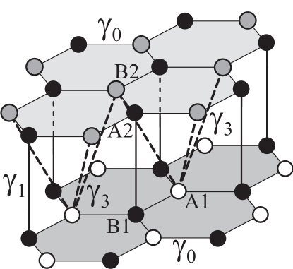
Figure 14: Schematic representation of the crystal structure of $AB$-stacked bilayer graphene illustrating skew interlayer coupling $\gamma_{3}$ (dashed lines) between $p_{z}$ orbitals on sites $A1$ (white) and $B2$ (grey)

The additional coupling is a skew interlayer coupling between $p_{z}$ orbitals on atomic sites $A1$ and $B2$, Fig. 14, denoted $\gamma_{3}$. For each $A1$ site, there are three $B2$ sites nearby. A calculation of the matrix element between $A1$ and $B2$ sites in the tight-binding model proceeds in a similar way as that between adjacent $A$ and $B$ sites in monolayer graphene, as described in Sect. 0.4.2. Then, the effective Hamiltonian in a basis with components $A1$, $B1$, $A2$, $B2$, for the four low-energy bands of bilayer graphene (100) is mcc06a :

$$H=\left(\begin{array}[]{cccc}0&-\gamma_{0}f\left(\mathbf{k}\right)&0&-\gamma_{3}f^{\ast}\left(\mathbf{k}\right)\\ -\gamma_{0}f^{\ast}\left(\mathbf{k}\right)&0&\gamma_{1}&0\\ 0&\gamma_{1}&0&-\gamma_{0}f\left(\mathbf{k}\right)\\ -\gamma_{3}f\left(\mathbf{k}\right)&0&-\gamma_{0}f^{\ast}\left(\mathbf{k}\right)&0\\ \end{array}\right)\,,$$ (167)

where

$$\gamma_{3}=-\langle\phi_{A1}\left(\mathbf{r}-\mathbf{R}_{A1}\right)|{\cal H}|\phi_{B2}\left(\mathbf{r}-\mathbf{R}_{B2}\right)\rangle\,.$$ (168)

The $\gamma_{3}$ term is relevant at low energy because it is a direct coupling between the $A1$ and $B2$ orbitals that form the two low-energy bands. Thus, using the linear-in-momentum approximation (77), terms such as $\gamma_{3}f\left(\mathbf{k}\right)\approx-v_{3}\left(\xi p_{x}-ip_{y}\right)$ appear in the two-component Hamiltonian written in basis ${c}_{A1}$, ${c}_{B2}$. Equation (113) is modified as mcc06a

$$\!\!\!\!\!\!H_{2,\xi}=v_{3}\!\left(\begin{array}[]{cc}0&\xi p_{x}+ip_{y}\\ \xi p_{x}-ip_{y}&0\\ \end{array}\right)\!-\!\frac{1}{2m}\!\left(\begin{array}[]{cc}0&\left(\xi p_{x}-ip_{y}\right)^{2}\\ \left(\xi p_{x}+ip_{y}\right)^{2}&0\\ \end{array}\right)\!\!,$$ (173)

where $v_{3}=\sqrt{3}a\gamma_{3}/(2\hbar)$ and $m=\gamma_{1}/(2v^{2})$. Taking into account trigonal warping, the low-energy Hamiltonian of bilayer graphene (173) resembles that of monolayer graphene (161). The principle difference lies in the magnitude of the parameters. Since $\gamma_{3}=0.315\,$eV dressel02 is an order of magnitude less than $\gamma_{0}=3.033\,$eV saito , then $v_{3}\ll v$. Thus, the linear term dominates in monolayers and the quadratic term dominates in bilayers over a broad range of energy. The energy eigenvalues of $H_{2,\xi}$, (173), are

$$E_{\pm}=\pm\sqrt{v_{3}^{2}p^{2}-\xi\frac{v_{3}p^{3}}{m}\cos 3\varphi+\left(\frac{p^{2}}{2m}\right)^{2}}\,,$$ (174)

for energies $|E_{\pm}|\ll\gamma_{1}$. Over a range of energy, the term independent of $v_{3}$ dominates, and the $v_{3}$ dependent terms produce trigonal warping of the isoenergetic line in the vicinity of each $K$ point. The effect of trigonal warping increases as the energy is lowered, until, at very low energies $E_{L}\approx{\textstyle\frac{1}{4}}\gamma_{1}(v_{3}/v)^{2}\approx 1\,$meV, it leads to a Lifshitz transition lif60 : the isoenergetic line breaks into four parts dre74 ; nak76 ; ino62 ; gup72 ; dressel02 ; mcc06a ; part06 ; mcc07 . There is one ‘central’ part, centered on the $K$ point ($p=0$), that is approximately circular with area $\mathcal{A}_{\mathrm{c}}\approx\pi E^{2}/(\hbar v_{3})^{2}$. In addition, there are three ‘leg’ parts that are elliptical with area $\mathcal{A}_{\mathrm{\ell}}\approx{\textstyle\frac{1}{3}}\mathcal{A}_{\mathrm{c}}$. Each ellipse has its major axis separated by angle $2\pi/3$ from the major axes of the other leg parts, as measured from the $K$ point, with the ellipse centered on $|p|=\gamma_{1}v_{3}/v^{2}$.

Here, we have described the low-energy band structure of monolayer and bilayer graphene within a simple tight-binding model, including a Lifshitz transition in bilayer graphene at very low energy $E_{L}\approx 1\,$meV. It is quite possible that electron-electron interactions have a dramatic effect on the band structure of bilayer graphene, producing qualitatively different features at low energy nil06 ; min08 ; zhangmin09 ; nand09 ; vafek10 ; lem10 .

0.10 Tuneable band gap in bilayer graphene

0.10.1 Asymmetry gap in the band structure of bilayer graphene

In graphene monolayers and bilayers, a combination of space and time inversion symmetry manes07 guarantees the existence of a gapless band structure exactly at the $K$ point, i.e. the $A$ and $B$ sublattices ($A1$ and $B2$ in bilayers) are identical, leading to degeneracy of the states they support at the $K$ point. Breaking inversion symmetry by, say, fixing the two sublattice sites to be at different energies, would lead to a gap between the conduction and valence bands at the $K$ point. In monolayer graphene, breaking the $A$/$B$ sublattice symmetry in a controllable way is very difficult: it would require a periodic potential because $A$ and $B$ are adjacent sites on the same layer. In bilayer graphene, however, the $A1$ and $B2$ sublattices lie on different layers and, thus, breaking the symmetry and opening a band gap may be achieved by doping or gating. Band-gap opening in bilayer graphene has recently been studied both theoretically mcc06a ; latil06 ; guinea06 ; mcc06b ; min07 ; aoki07 ; gava ; castro ; zhang08 ; fogler10 and in a range of different experiments ohta06 ; oostinga ; castro ; zhang08 ; hen08 ; li08 ; zhang09 ; mak09 ; kuz09a ; kuz09b ; kuz09c ; zhao10 ; kim10 .

If we introduce an asymmetry parameter $\Delta=\epsilon_{2}-\epsilon_{1}$ describing the difference between on-site energies in the two layers, $\epsilon_{A2}=\epsilon_{B2}=\epsilon_{2}={\textstyle\frac{1}{2}}\Delta$, $\epsilon_{A1}=\epsilon_{B1}=\epsilon_{1}=-{\textstyle\frac{1}{2}}\Delta$, then the transfer integral matrix of bilayer graphene (90), in a basis with components $A1$, $B1$, $A2$, $B2$, becomes mcc06a ; guinea06 ; mcc06b

$$H = \left(\begin{array}[]{cccc}-{\textstyle\frac{1}{2}}\Delta&-\gamma_{0}f\left(\mathbf{k}\right)&0&0\\ -\gamma_{0}f^{\ast}\left(\mathbf{k}\right)&-{\textstyle\frac{1}{2}}\Delta&\gamma_{1}&0\\ 0&\gamma_{1}&{\textstyle\frac{1}{2}}\Delta&-\gamma_{0}f\left(\mathbf{k}\right)\\ 0&0&-\gamma_{0}f^{\ast}\left(\mathbf{k}\right)&{\textstyle\frac{1}{2}}\Delta\\ \end{array}\right)\,,$$ (179)

The band structure may be determined by solving the secular equation $\det\left(H-E_{j}S\right)=0$ using overlap matrix $S$, (95). It is plotted in Fig. 15 for parameter values $\gamma_{0}=3.033\,$eV, $s_{0}=0.129$ and $\Delta=\gamma_{1}=0.39\,$eV. A band gap appears between the conduction and valence bands near the $K$ points (left inset in Fig. 15).

Figure 15: The low-energy band structure of bilayer graphene in the presence of interlayer asymmetry $\Delta$. Parameter values are $\gamma_{0}=3.033\,$eV, $s_{0}=0.129$, $\Delta=\gamma_{1}=0.39\,$eV. The plot shows the bands calculated along the $k_{x}$ axis intersecting points $K_{-}$, $\Gamma$, and $K_{+}$ in the Brillouin zone, shown as the dotted line in the right inset. The left inset shows the band structure in the vicinity of the point $K_{-}$.

To develop an analytic description of the bands at low energy, we neglect non-orthogonality of the orbitals on adjacent sites, so that the overlap matrix $S$, (95), becomes a unit matrix. Then, the bands at low energy are described by Hamiltonian, (179), with eigenvalues mcc06a given by

$$E_{\pm}^{(\alpha)}=\pm\left[\frac{\Delta^{2}}{4}+v^{2}p^{2}+\frac{\gamma_{1}^{2}}{2}+\alpha\frac{\gamma_{1}^{2}}{2}\sqrt{1+\frac{4v^{2}p^{2}}{\gamma_{1}^{2}}+\frac{4\Delta^{2}v^{2}p^{2}}{\gamma_{1}^{4}}}\right]^{1/2}\!\!\!\!\!\!,$$ (180)

where $\alpha=1$ for the split bands and $\alpha=-1$ for the low-energy bands. Here, we used the linear approximation $f\left(\mathbf{k}\right)\approx-v\left(\xi p_{x}-ip_{y}\right)/\gamma_{0}$, (77), so that $\gamma_{0}|f\left(\mathbf{k}\right)|\approx vp$. Eigenvalues $E_{\pm}^{(-1)}$ describe the low-energy bands split by a gap. They have a distinctive ‘Mexican hat’ shape, shown in the left inset in Fig. 15. The separation between the bands exactly at the $K$ point, $E_{+}^{(-1)}(p=0)-E_{-}^{(-1)}(p=0)$, is equal to $|\Delta|$, but the true value of the band gap $\Delta_{g}$ occurs at non-zero value of the momentum $p_{g}$ away from the $K$ point,

$$p_{g} = \frac{|\Delta|}{2v}\sqrt{\frac{\Delta^{2}+2\gamma_{1}^{2}}{\Delta^{2}+\gamma_{1}^{2}}}\,,$$ (181)

$$\Delta_{g} = E_{+}^{(-1)}(p_{g})-E_{-}^{(-1)}(p_{g})=\frac{|\Delta|\gamma_{1}}{\sqrt{\Delta^{2}+\gamma_{1}^{2}}}\,.$$ (182)

For moderate values of the asymmetry parameter, $|\Delta|\ll\gamma_{1}$, then the band gap $\Delta_{g}\approx|\Delta|$, but for extremely large values, $|\Delta|\gg\gamma_{1}$, the gap saturates $\Delta_{g}\approx\gamma_{1}$, where $\gamma_{1}$ is of the order of three to four hundred meV. The value of the asymmetry parameter $\Delta$ and bandgap $\Delta_{g}$ may be tuned using an external gate potential, but the ability of an external gate to induce a potential asymmetry between the layers of the bilayer depends on screening by the electrons in bilayer graphene, as discussed in the following.

0.10.2 Self-consistent model of screening in bilayer graphene

Introduction

The influence of screening on band-gap opening in bilayer graphene has been modeled using the tight-binding model and Hartree theory mcc06b ; min07 ; castro ; zhang08 ; fogler10 , and this simple analytic model is in good qualitative agreement with density functional theory min07 ; gava and experiments castro ; li08 ; zhang08 ; mak09 ; kuz09b . Recently, the tight-binding model and Hartree theory approach has been applied to graphene trilayers and multilayers kosh09a ; avet ; avet2 ; kosh10a . Here, we review the tight-binding model and Hartree theory approach which provides analytical formulae that serve to illustrate the pertinent physics. We will use the SI system of units throughout, and adopt the convention that the charge of the electron is $-e$ where the quantum of charge $e>0$.

Using elementary electrostatics, it is possible to relate the asymmetry parameter $\Delta=\epsilon_{2}-\epsilon_{1}$ to the distribution of electronic density over the bilayer system in the presence of external gates, but the density itself depends explicitly on $\Delta$ because of the effect $\Delta$ has on the band structure, (180). Therefore, the problem requires a self-consistent calculation of density and $\Delta$, leading to a determination of the gate-dependence of the gap $\Delta_{g}$.

The model assumes that bilayer graphene consists of two parallel conducting plates located at $x=-c_{0}/2$ and $+c_{0}/2$, where $c_{0}$ is the interlayer spacing, as illustrated in Fig. 16. The two layers support electron densities $n_{1}$, $n_{2}$, respectively, corresponding to charge densities $\sigma_{1}=-en_{1}$, $\sigma_{2}=-en_{2}$, and the permittivity of the bilayer interlayer space is $\varepsilon_{r}$ (neglecting the screening effect of $\pi$-band electrons that we explicitly take into account here). We consider the combined effect of a back and top gate, with the back (top) gate at $x=-L_{b}$ ($x=+L_{t}$), held at potential $V_{b}$ ($V_{t}$), separated from the bilayer by a dielectric medium with relative permittivity $\varepsilon_{b}$ ($\varepsilon_{t}$). In addition, we include the influence of additional background charge near the bilayer with density $n_{b0}$ on the back-gate side and $n_{t0}$ on the top-gate side, yielding charge densities $\sigma_{b0}=en_{b0}$ and $\sigma_{t0}=en_{t0}$ where $n_{b0}$ and $n_{t0}$ are positive for positive charge.

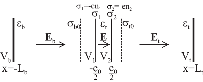
Figure 16: Schematic of bilayer graphene in the presence of back and top gates. Bilayer graphene consists of two parallel conducting plates with respective electron densities $n_{1}$, $n_{2}$ located at $x=-c_{0}/2$ and $+c_{0}/2$, respectively, where $c_{0}$ is the interlayer spacing, and $\varepsilon_{r}$ is the permittivity of the bilayer interlayer space. The back (top) gate at $x=-L_{b}$ ($x=+L_{t}$), held at potential $V_{b}$ ($V_{t}$), is separated from the bilayer by a dielectric medium with relative permittivity $\varepsilon_{b}$ ($\varepsilon_{t}$). Dashed lines indicate additional background charge near the bilayer with charge densities $\sigma_{b0}$ and $\sigma_{t0}$ on the back-gate and top-gate side, respectively.

Electrostatics

Applying Gauss’s Law firstly to a Gaussian surface enclosing cross-sectional area $A$ of both layers of the bilayer and, secondly, to a Gaussian surface enclosing one layer only yields

$$-\varepsilon_{0}\varepsilon_{b}E_{b}A+\varepsilon_{0}\varepsilon_{t}E_{t}A = -e\left(n_{1}+n_{2}-n_{b0}-n_{t0}\right)A\,,$$ (183)

$$-\varepsilon_{0}\varepsilon_{r}EA+\varepsilon_{0}\varepsilon_{t}E_{t}A = -e\left(n_{2}-n_{t0}\right)A\,.$$ (184)

The electric fields may be related to potential differences,

$$E_{b} \approx V_{b}/L_{b}\,,\qquad E_{t}\approx-V_{t}/L_{t}\,,$$ (185)

$$E \approx \left(V_{1}-V_{2}\right)/c_{0}\equiv\Delta/(ec_{0})\,.$$ (186)

and, when substituted into (183) and (184), they give

$$n=n_{1}+n_{2} = \frac{\varepsilon_{0}\varepsilon_{b}V_{b}}{eL_{b}}+\frac{\varepsilon_{0}\varepsilon_{t}V_{t}}{eL_{t}}+n_{b0}+n_{t0}\,,$$ (187)

$$\Delta = -\frac{\varepsilon_{t}}{\varepsilon_{r}}\frac{c_{0}}{L_{t}}eV_{t}+\frac{e^{2}c_{0}}{\varepsilon_{0}\varepsilon_{r}}\left(n_{2}-n_{t0}\right)\,.$$ (188)

The first equation, (187), relates the total density of $\pi$-band electrons $n=n_{1}+n_{2}$ on the bilayer to the gate potentials, generalizing the case of monolayer graphene novo04 . The second equation, (188), gives the value of the asymmetry parameter. Using (187), it may be written in a slightly different way:

$$\Delta = \Delta_{\mathrm{ext}}+\Lambda\gamma_{1}\frac{\left(n_{2}-n_{1}\right)}{n_{\perp}}\,,$$ (189)

$$\Delta_{\mathrm{ext}} = \frac{1}{2}\frac{\varepsilon_{b}}{\varepsilon_{r}}\frac{c_{0}}{L_{b}}eV_{b}-\frac{1}{2}\frac{\varepsilon_{t}}{\varepsilon_{r}}\frac{c_{0}}{L_{t}}eV_{t}+\Lambda\gamma_{1}\frac{\left(n_{b0}-n_{t0}\right)}{n_{\perp}}\,,$$ (190)

where parameters $n_{\perp}$ and $\Lambda$ are defined as

$$n_{\perp}=\frac{\gamma_{1}^{2}}{\pi\hbar^{2}v^{2}}\,,\qquad\Lambda=\frac{c_{0}e^{2}\gamma_{1}}{2\pi\hbar^{2}v^{2}\varepsilon_{0}\varepsilon_{r}}\equiv\frac{c_{0}e^{2}n_{\perp}}{2\gamma_{1}\varepsilon_{0}\varepsilon_{r}}\,.$$ (191)

The first term in (189) is $\Delta_{\mathrm{ext}}$, the value of $\Delta$ if screening were negligible, as determined by a difference between the gate potentials, (190). Equations (187,190) show that the effect of the background densities $n_{b0}$ and $n_{t0}$ may be absorbed in a shift of the gate potentials $V_{b}$ and $V_{t}$, respectively.

The second term in (189) indicates the influence of screening by electrons on the bilayer where $n_{\perp}$ is the characteristic density scale and $\Lambda$ is a dimensionless parameter indicating the strength of interlayer screening. Using $\gamma_{1}=0.39$eV and $v=1.0\times 10^{6}$ms^-1 gives $n_{\perp}=1.1\times 10^{13}$cm^-2. For interlayer spacing $c_{0}=3.35$Å and dielectric constant $\varepsilon_{r}\approx 1$, then $\Lambda\sim 1$, indicating that screening is an important effect.

Layer densities

Equation (189) uses electrostatics to relate $\Delta$ to the electronic densities $n_{1}$ and $n_{2}$ on the individual layers. The second ingredient of the self-consistent analysis are expressions for $n_{1}$ and $n_{2}$ in terms of $\Delta$, taking into account the electronic band structure of bilayer graphene. The densities are determined by an integral with respect to momentum over the circular Fermi surface

$$n_{1(2)}=\frac{2}{\pi\hbar^{2}}\int p\,dp\left[|\psi_{A1(2)}(p)|^{2}+|\psi_{B1(2)}(p)|^{2}\right]$$ (192)

where a factor of four is included to take into account spin and valley degeneracy. Using the four-component Hamiltonian (179), with linear approximation $f\left(\mathbf{k}\right)\approx-v\left(\xi p_{x}-ip_{y}\right)/\gamma_{0}$, it is possible to determine the wave function amplitudes on the four atomic sites mcc06b to find

$$\!\!\!n_{1(2)} = \int dp\,p\!\left(\frac{E\mp\Delta/2}{\pi\hbar^{2}E}\right)\!\!\!\left[\frac{\left(E^{2}-\Delta^{2}/4\right)^{2}\mp 2v^{2}p^{2}E\Delta-v^{4}p^{4}}{\left(E^{2}-\Delta^{2}/4\right)^{2}+v^{2}p^{2}\Delta^{2}-v^{4}p^{4}}\right]\!\!,$$ (193)

where the minus (plus) sign is for the first (second) layer and $E$ is the band energy.

For simplicity, we consider the Fermi level to lie within the lower conduction band, but above the Mexican hat region, $|\Delta|/2<E_{F}\ll\gamma_{1}$. We approximate the dispersion relation, (180), as $E_{+}^{(-1)}\approx\sqrt{\Delta^{2}/4+v^{4}p^{4}/\gamma_{1}^{2}}$ which neglects features related to the Mexican hat. Then, the contribution to the layer densities from the partially-filled conduction band mcc06b ; fogler10 is given by

$$n_{1(2)}^{\mathrm{cb}}\approx\frac{n}{2}\mp\frac{n_{\perp}\Delta}{4\gamma_{1}}\ln\left(\frac{2|n|\gamma_{1}}{n_{\perp}|\Delta|}+\sqrt{1+\left(\frac{2n\gamma_{1}}{n_{\perp}\Delta}\right)^{2}}\right)\,,$$ (194)

where the total density $n=p_{F}^{2}/\pi\hbar^{2}$. In addition, although the filled valence band doesn’t contribute to a change in the total density $n$, it contributes towards the finite layer polarization in the presence of finite $\Delta$ which, to leading order in $\Delta$, is given by

$$n_{1(2)}^{\mathrm{vb}}\approx\pm\frac{n_{\perp}\Delta}{4\gamma_{1}}\ln\left(\frac{4\gamma_{1}}{|\Delta|}\right)\,.$$ (195)

Then, the total layer density, $n_{1(2)}=n_{1(2)}^{\mathrm{cb}}+n_{1(2)}^{\mathrm{vb}}$, is given by

$$n_{1(2)}\approx\frac{n}{2}\mp\frac{n_{\perp}\Delta}{4\gamma_{1}}\ln\left(\frac{|n|}{2n_{\perp}}+\frac{1}{2}\sqrt{\left(\frac{n}{n_{\perp}}\right)^{2}+\left(\frac{\Delta}{2\gamma_{1}}\right)^{2}}\right)\,.$$ (196)

Self-consistent screening

The density-dependence of the asymmetry parameter $\Delta$ and band gap $\Delta_{g}$ are determined mcc06b ; fogler10 by substituting the expression for the layer density, (196), into (189):

$$\Delta\left(n\right)\approx\Delta_{\mathrm{ext}}\left[1-\frac{\Lambda}{2}\ln\left(\frac{|n|}{2n_{\perp}}+\frac{1}{2}\sqrt{\left(\frac{n}{n_{\perp}}\right)^{2}+\left(\frac{\Delta}{2\gamma_{1}}\right)^{2}}\right)\right]^{-1}\,,$$ (197)

with $\Delta_{\mathrm{ext}}$ given by (190). The logarithmic term describes the influence of screening: when this term is much smaller than unity, screening is negligible and $\Delta\approx\Delta_{\mathrm{ext}}$, whereas when the logarithmic term is much larger than unity, screening is strong, $|\Delta|\ll|\Delta_{\mathrm{ext}}|$. The magnitude of the logarithmic term is proportional to the screening parameter $\Lambda$. As discussed earlier, $\Lambda\sim 1$ in bilayer graphene, so it is necessary to take account of the density dependence of the logarithmic term in (197).

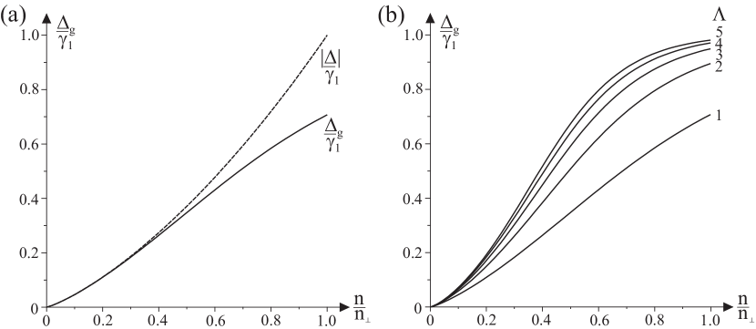
Figure 17: Density-dependence of the band gap $\Delta_{g}$ in bilayer graphene, in the presence of a single back gate: (a) asymmetry parameter $\Delta$ and gap $\Delta_{g}=|\Delta|\gamma_{1}/\sqrt{\Delta^{2}+\gamma_{1}^{2}}$ for screening parameter $\Lambda=1$; (b) band gap $\Delta_{g}$ for different values of the screening parameter. Plots were made using Eqs. (182) and (198).

To understand the density dependence of $\Delta$, let us consider bilayer graphene in the presence of a single back gate, $V_{t}=n_{b0}=n_{t0}=0$. This is a common situation for experiments with exfoliated graphene on a silicon substrate novo04 ; novo05 ; zhang05 ; novo06 . Then, the relation between density and gate voltage, (187), becomes the same as in monolayer graphene novo04 , $n=\varepsilon_{0}\varepsilon_{b}V_{b}/(eL_{b})$. The expression for $\Delta_{\mathrm{ext}}$, (190), reduces to $\Delta_{\mathrm{ext}}=\Lambda\gamma_{1}n/n_{\perp}$, and the expression for $\Delta\left(n\right)$, (197), simplifies mcc06b as

$$\Delta\left(n\right)\approx\frac{\Lambda\gamma_{1}n}{n_{\perp}}\left[1-\frac{\Lambda}{2}\ln\left(\frac{|n|}{n_{\perp}}\right)\right]^{-1}\,,$$ (198)

The value of the true band gap $\Delta_{g}(n)$ may be obtained using (182), $\Delta_{g}=|\Delta|\gamma_{1}/\sqrt{\Delta^{2}+\gamma_{1}^{2}}$. Asymmetry parameter $\Delta(n)$ and band gap $\Delta_{g}(n)$ are plotted in Fig. 17 as a function of density $n$. For large density, $|n|\sim n_{\perp}$, the logarithmic term in (198) is negligible and the asymmetry parameter is approximately linear in density, $\Delta(n)\approx\Lambda\gamma_{1}n/n_{\perp}$. At low density, $|n|\ll n_{\perp}$, the logarithmic term is large, indicating that screening is strong, and the asymmetry parameter approaches $\Delta(n)\approx 2\gamma_{1}(n/n_{\perp})/\ln(n_{\perp}/|n|)$. The comparison of $\Delta(n)$ and $\Delta_{g}(n)$, Fig. 17(a), shows that, at low density $|n|\ll n_{\perp}$, $\Delta_{g}(n)\approx|\Delta(n)|$ and, asymptotically, $\Delta_{g}(n)\approx 2\gamma_{1}(|n|/n_{\perp})/\ln(n_{\perp}/|n|)$. This is independent of the screening parameter $\Lambda$ [see Fig. 17(b)]. The curves for different values of the screening parameter $\Lambda$, Fig. 17(b), illustrate that, even when $|\Delta|$ is very large, $|\Delta|\gg\gamma_{1}$, $\Delta_{g}$ saturates at the value of $\gamma_{1}$.

In deriving the above expression for $\Delta\left(n\right)$, a number of approximations were made including simplifying the band structure [by omitting features related to the Mexican hat or to other possible terms in the Hamiltonian (179)], neglecting screening due to other orbitals, and neglecting the effects of disorder and electron-electron exchange and correlation. Nevertheless, it seems to be in good qualitative agreement with density functional theory calculations min07 ; gava and experiments (see, for example, castro ; li08 ; zhang08 ; mak09 ; kuz09b ).

0.11 Summary

In this Chapter, some of the electronic properties of monolayer and bilayer graphene were described using the tight-binding model. Effective Hamiltonians for low-energy electrons were derived, corresponding to massless chiral fermions in monolayers and massive chiral fermions in bilayers. Chirality in graphene is manifest in many electronic properties, including anisotropic scattering and an unusual sequence of plateaus in the quantum Hall effect. There are a number of additional contributions to the low-energy Hamiltonians of graphene that influence chiral electrons and we focused on one of them, trigonal warping, here.

Comparison with experiments suggest that the tight-binding model generally works very well in graphene. The model contains parameters, corresponding to the energies of atomic orbitals or to matrix elements describing hopping between atomic sites, that cannot be determined by the model. They must be estimated by an alternative theoretical method, such as density-functional theory, or they can be treated as fitting parameters to be determined by comparison with experiments. The simple model described in this Chapter is versatile and it serves as the starting point for a wide range of models encapsulating advanced physical phenomena, including interaction effects, and the tight-binding model may be used to describe the electronic structure of multilayer graphene, too. Here, we described a different example: the use of the tight-binding model with Hartree theory to develop a simple model of screening by electrons in bilayer graphene in order to calculate the density dependence of the band gap induced by an external electric field.

Acknowledgments

The author thanks colleagues for fruitful collaboration in graphene research, in particular V.I. Fal’ko, and EPSRC for financial support.

References

- (1) P.R. Wallace, Phys. Rev. 71, 622 (1947)
- (2) J.C. Slonczewski, P.R. Weiss, Phys. Rev. 109, 272 (1958)
- (3) J.W. McClure, Phys. Rev. 108, 612 (1957)
- (4) M.S Dresselhaus, G. Dresselhaus, Adv. Phys. 51, 1 (2002)
- (5) D.P. DiVincenzo, E.J. Mele, Phys. Rev. B 29, 1685 (1984)
- (6) J. González, F. Guinea, M.A.H. Vozmediano, Phys. Rev. Lett. 69, 172 (1992).
- (7) H. Ajiki, T. Ando, J. Phys. Soc. Jpn. 62, 1255 (1993)
- (8) C.L. Kane, E.J. Mele, Phys. Rev. Lett. 78, 1932 (1997)
- (9) T. Ando, T. Nakanishi, R. Saito, J. Phys. Soc. Jpn. 67, 2857 (1998).
- (10) P.L. McEuen, M. Bockrath, D.H. Cobden, Y.-G. Yoon, S.G. Louie, Phys. Rev. Lett. 83, 5098 (1999)
- (11) R. Saito, M.S. Dresselhaus, G. Dresselhaus Physical Properties of Carbon Nanotubes, (Imperial College Press, London, 1998)
- (12) G.W. Semenoff, Phys. Rev. Lett. 53, 2449 (1984)
- (13) F.D.M. Haldane, Phys. Rev. Lett. 61, 2015 (1988)
- (14) K.S. Novoselov, A.K. Geim, S.V. Morozov, D. Jiang, Y. Zhang, S.V. Dubonos, I.V. Grigorieva, A.A. Firsov, Science 306, 666 (2004)
- (15) K.S. Novoselov, A.K. Geim, S.V. Morozov, D. Jiang, M.I. Katsnelson, I.V. Grigorieva, S.V. Dubonos, A.A. Firsov, Nature 438, 197 (2005)
- (16) Y.B. Zhang, Y.W. Tan, H.L. Stormer, P. Kim, Nature 438, 201 (2005)
- (17) K.S. Novoselov, E. McCann, S.V. Morozov, I.V. Fal’ko, M.I. Katsnelson, U. Zeitler, D. Jiang, F. Schedin, A.K. Geim, Nature Phys. 2 177 (2006)
- (18) N.W. Ashcroft, N.D. Mermin, Solid-State Physics, (Brooks/Cole, Belmont, 1976)
- (19) A.H. Castro Neto, F. Guinea, N.M.R. Peres, K.S. Novoselov, A.K. Geim, Rev. Mod. Phys. 81, 109 (2009)
- (20) C. Bena, G. Montambaux, New J. Phys. 11, 095003 (2009)
- (21) E. McCann, V.I. Fal’ko, Phys. Rev. Lett. 96, 086805 (2006)
- (22) G. Dresselhaus, Phys. Rev. B 10, 3602 (1974)
- (23) K. Nakao, J. Phys. Soc. Japan 40, 761 (1976)
- (24) M. Inoue, J. Phys. Soc. Japan 17, 808 (1962)
- (25) O.P. Gupta, P.R. Wallace, Phys. Status. Solidi. B 54, 53 (1972)
- (26) T. Ohta, A. Bostwick, T. Seyller, K. Horn, E. Rotenberg, Science 313, 951 (2006)
- (27) J.B. Oostinga, H.B. Heersche, X. Liu, A.F. Morpurgo, L.M.K. Vandersypen, Nature Materials 7, 151 (2007)
- (28) E. McCann, Phys. Rev. B 74, 161403(R) (2006)
- (29) K. Sasaki, S. Murakami, R. Saito, Appl. Phys. Lett. 88, 113110 (2006)
- (30) N.M.R. Peres, F. Guinea, A.H. Castro Neto, Phys. Rev. B 73, 125411 (2006)
- (31) S. Pancharatnam, Proc. Indian Acad. Sci. A 44, 247 (1956)
- (32) M.V. Berry, Proc. R. Soc. Lond. A 392, 45 (1984)
- (33) H. Suzuura, T. Ando, Phys. Rev. Lett. 89, 266603 (2002)
- (34) V.V. Cheianov, V.I. Fal ko, Phys. Rev. B 74, 041403(R) (2006)
- (35) M.I. Katsnelson, K.S. Novoselov, A.K. Geim, Nature Phys. 2, 620 (2006)
- (36) S.B. Trickey, F. Müller-Plathe, G.H.F. Diercksen, J.C. Boettger, Phys. Rev. B 45, 4460 (1992)
- (37) V.I. Fal ko, K. Kechedzhi, E. McCann, B.L. Altshuler, H. Suzuura, T. Ando, Solid State Comm. 143 33 (2007)
- (38) J.R. Schrieffer, P. A. Wolff, Phys. Rev. 149, 491 (1966)
- (39) L.D. Landau, Z. Phys. 64, 629 (1930)
- (40) K. von Klitzing, G. Dorda, M. Pepper, Phys. Rev. Lett. 45, 494 (1980)
- (41) R.E. Prange, S.M. Girvin (eds.), The Quantum Hall Effect, (Springer-Verlag, New York, 1986)
- (42) A.H. MacDonald (ed.), Quantum Hall Effect: A Perspective, (Kluwer, Boston, 1989)
- (43) J.W. McClure, Phys. Rev. 104, 666 (1956)
- (44) H.J. Fischbeck, Phys. Status Solidi 38, 11 (1970)
- (45) Y. Zheng, T. Ando, Phys. Rev. B 65, 245420 (2002)
- (46) V.P. Gusynin, S.G. Sharapov, Phys. Rev. Lett. 95, 146801 (2005)
- (47) I.F. Herbut, Phys. Rev. B 75, 165411 (2007)
- (48) L.M. Lifshitz, Zh. Exp. Teor. Fiz. 38, 1565 (1960) [Sov. Phys. JETP 11, 1130 (1960)]
- (49) B. Partoens, F.M. Peeters, Phys. Rev. B 74, 075404 (2006)
- (50) E. McCann, D.S.L. Abergel, V.I. Fal ko, Solid State Comm. 143, 110 (2007)
- (51) J. Nilsson, A.H. Castro Neto, N.M.R. Peres, F. Guinea, Phys. Rev. B 73, 214418 (2006)
- (52) H. Min, G. Borghi, M. Polini, A.H. MacDonald, Phys. Rev. B 77, 041407(R) (2008)
- (53) F. Zhang, H. Min, M. Polini, A.H. MacDonald, Phys. Rev. B 81, 041402(R) (2010)
- (54) R. Nandkishore, L.S. Levitov, Phys. Rev. Lett. 104, 156803 (2010)
- (55) O. Vafek, K. Yang, Phys. Rev. B 81, 041401(R) (2010)
- (56) Y. Lemonik, I.L. Aleiner, C. Toke, V.I. Fal’ko, Phys. Rev. B 82, 201408 (2010)
- (57) J.L. Manes, F. Guinea, M.A.H. Vozmediano, Phys. Rev. B 75, 155424 (2007)
- (58) S. Latil, L. Henrard, Phys. Rev. Lett. 97, 036803 (2006)
- (59) F. Guinea, A.H. Castro Neto, N.M.R. Peres, Phys. Rev. B 73, 245426 (2006)
- (60) H. Min, B.R. Sahu, S.K. Banerjee, A.H. MacDonald, Phys. Rev. B 75, 155115 (2007)
- (61) M. Aoki, H. Amawashi, Solid State Commun. 142, 123 (2007)
- (62) E.V. Castro, K.S. Novoselov, S.V. Morozov, N.M.R. Peres, J.M.B. Lopes dos Santos, J. Nilsson, F. Guinea, A.K. Geim, A.H. Castro Neto, Phys. Rev. Lett. 99, 216802 (2007)
- (63) L.M. Zhang, Z.Q. Li, D.N. Basov, M.M. Fogler, Z. Hao, M.C. Martin, Phys. Rev. B 78, 235408 (2008)
- (64) P. Gava, M. Lazzeri, A.M. Saitta, F. Mauri, Phys. Rev. B 79, 165431 (2009)
- (65) M.M. Fogler, E. McCann, Phys. Rev. B 82, 197401 (2010)
- (66) E.A. Henriksen, Z. Jiang, L.-C. Tung, M.E. Schwartz, M. Takita, Y.-J. Wang, P. Kim, H.L. Stormer, Phys. Rev. Lett. 100, 087403 (2008)
- (67) Z.Q. Li, E.A. Henriksen, Z. Jiang, Z. Hao, M.C. Martin, P. Kim, H.L. Stormer, D.N. Basov, Phys. Rev. Lett. 102, 037403 (2009)
- (68) Y. Zhang, T.-T. Tang, C. Girit, Z. Hao, M.C. Martin, A. Zettl, M.F. Crommie, Y.R. Shen, F. Wang, Nature 459, 820 (2009)
- (69) K.F. Mak, C.H. Lui, J. Shan, T.F. Heinz, Phys. Rev. Lett. 102, 256405 (2009)
- (70) A.B. Kuzmenko, E. van Heumen, D. van der Marel, P. Lerch, P. Blake, K.S. Novoselov, A.K. Geim, Phys. Rev. B 79, 115441 (2009)
- (71) A.B. Kuzmenko, I. Crassee, D. van der Marel, P. Blake, K.S. Novoselov, Phys. Rev. B 80, 165406 (2009)
- (72) A.B. Kuzmenko, L. Benfatto, E. Cappelluti, I. Crassee, D. van der Marel, P. Blake, K.S. Novoselov, A. K. Geim, Phys. Rev. Lett. 103, 116804 (2009)
- (73) Y. Zhao, P. Cadden-Zimansky, Z. Jiang, P. Kim, Phys. Rev. Lett. 104, 066801 (2010)
- (74) S. Kim, K. Lee, E. Tutuc, Phys. Rev. Lett. 107, 016803 (2011)
- (75) M. Koshino, E. McCann, Phys. Rev. B 79, 125443 (2009)
- (76) A.A Avetisyan, B. Partoens, F.M. Peeters, Phys. Rev. B 79, 035421 (2009)
- (77) A.A Avetisyan, B. Partoens, F.M. Peeters, Phys. Rev. B 80, 195401 (2009)
- (78) M. Koshino, Phys. Rev. B 81, 125304 (2010)