Assessing the behavior of modern solar magnetographs and spectropolarimeters

Abstract

The design and later use of modern spectropolarimeters and magnetographs require a number of tolerance specifications that allow the developers to build the instrument and then the scientists to interpret the data accuracy. Such specifications depend both on device-specific features and on the physical assumptions underlying the particular measurement technique. Here we discuss general properties of every magnetograph, as the detectability thresholds for the vector magnetic field and the line-of-sight velocity, as well as specific properties of a given type of instrument, namely that based on a pair of nematic liquid crystal variable retarders and a Fabry-Pérot etalon (or several) for carrying out the light polarization modulation and spectral analysis, respectively. We derive formulae that give the detection thresholds in terms of the signal-to-noise ratio of the observations and the polarimetric efficiencies of the instrument. Relationships are also established between inaccuracies in the solar physical quantities and instabilities in the instrument parameters. Such relationships allow, for example, to translate scientific requirements for the velocity or the magnetic field into requirements for temperature or voltage stability. We also demonstrate that this type of magnetograph can theoretically reach the optimum polarimetric efficiencies of an ideal polarimeter, regardless of the optics in between the modulator and the analyzer. Such optics induces changes in the instrument parameters that are calculated too.

1. Introduction

Spectropolarimetry and magnetography have become two of the most useful tools in solar physics because they provide the deepest analysis one can make of light. Solar information is encoded in the spectrum of the Stokes parameters. We measure this spectrum and infer solar quantities from it. Recently, less and less conceptual differences exist between spectropolarimeters and magnetographs except for the specific devices: the formers usually include those instruments using a scanning spectrograph; the latter usually employ a bidimensional filtergraph like a Fabry-Pérot etalon. Some decades ago magnetographs were only able to sample one or two wavelengths across a spectral line; nowadays, new technologies provide a better wavelength sampling, thus enabling the scientists to interpret the data in terms of sophisticated inversion techniques of the radiative transfer equation, a procedure similar to the one regularly used with spectropolarimeters. Some of the instruments mentioned below enter this category. Modern solar spectropolarimeters and magnetographs are often vectorial because all four Stokes parameters of the light spectrum are measured. Longitudinal magnetography (i.e., Stokes $I\pm V$) can be interesting for some specific applications, but the partial analysis is usually included (if possible) as a particular case of the more general, full-Stokes polarimetry. Some of these modern instruments have been recently built or are currently in operation (e.g., the Tenerife Infrared Polarimeter, TIP, Martínez Pillet et al. 1999, Collados et al. 2007; the Diffraction-Limited Spectro-Polarimeter, DLSP, Sankarasubramanian et al. 2003; the air-spaced Fabry-Perot based CRISP instrument, Scharmer et al. 2008; the spectropolarimeter, SP, Lites et al. 2001, for the Hinode mission, Kosugi et al. 2007; CRISP, Narayan et al. 2008; the Visible Imaging Polarimeter, VIP, Beck et al. 2010; the Imaging Magnetograph eXperiment, IMaX, Martínez Pillet et al. 2011, for the Sunrise mission, Barthol et al. 2011; and the Helioseismic and Magnetic Imager, HMI, Graham et al. 2003, for the Solar Dynamics Observatory mission, Title 2000). Some other are being designed and built for near future operation and missions (e.g., the Polarimetric and Helioseismic Imager, SO/PHI, [formerly called VIM, Martínez Pillet 2007] for the Solar Orbiter mission, Marsch et al. 2005).

The common interest of users of these instruments is centered in vector magnetic fields (of components $B$, $\gamma$, and $\phi$) and line-of-sight (LOS) velocities ($v_{\rm LOS}$). Some spectropolarimeters can provide information on temperatures as well (and eventually on another thermodynamical quantity) but that feature is not common to all of them. Therefore, assessing the magnetograph capabilities in terms of their accuracy for retrieving magnetographic and tachographic quantities is in order since such an analysis can diagnose how far reaching is our current knowledge of the solar dynamics and magnetism. The diagnostics is relevant both for the design of new instruments in order to maximize their performances and for the analysis of uncertainties in data coming from currently operating devices. General considerations can obviously not be made but a few. Specifically, we here study in Sect. 2 the detection thresholds induced by random noise on the inferred longitudinal and transverse components of the magnetic field; in the particular case of photon-induced noise we also find uncertainty formulas. Both thresholds and relative uncertainties are obtained in terms of the signal-to-noise ratio of the observations and of the polarimetric efficiencies of the instrument. Since such efficiencies vary from instrument to instrument, at that point, the analysis concentrates in a particular type of magnetograph, namely that consisting of two nematic liquid crystal variable retarders (LCVRs) as the polarization modulator and a Fabry-Pérot etalon. In Sect. 3, we demonstrate that these polarimeters can reach the theoretically optimum efficiencies no matter the optics behind the modulator, including the etalon. The way for calculating the required retardances for the two LCVRs are explained along with a number of rules and periodicities in the solutions. Section 4 analyzes these instruments in terms of the influence of temperature and voltage instabilities, as well as of thickness inhomogeneities (roughness), of both the LCVRs and the etalon(s), on the final magnetographic and tachographic measurements. Finally, Sect. 5 summarizes the results.

2. The thresholding action of random noise

Most astrophysical measurements are nothing but photon counting. Their accuracy, therefore, depends on photometric accuracy, that is, on a battle between our ability to detect changes in the solar (stellar) physical quantities and the noise that hide such changes. The key concept is changes: we need to discern if a given quantity like the magnetic field strength, $B$, or the line-of-sight (LOS) velocity, $v_{\rm LOS}$, varies among pixels: whether or not it is greater or smaller than in the neighbor zones. The only tool we have to gauge these changes is the observable Stokes parameter changes that are linked to them through the response functions. Discussing response functions is out of the scope of this paper as they have been extensively analyzed elsewhere (e.g., Del Toro Iniesta et al., 2010; Orozco Suárez & Del Toro Iniesta, 2007; Del Toro Iniesta, 2003; Del Toro Iniesta & Ruiz Cobo, 1996; Ruiz Cobo & Del Toro Iniesta, 1994; Landi Degl’Innocenti & Landi Degl’Innocenti, 1977; Mein, 1971). As explained by Del Toro Iniesta & Martínez Pillet (2010), purely phenomenological approaches (e.g., Cabrera Solana et al., 2005) are also valid to establish a relationship between changes in the physical quantities and the Stokes parameters. Here we shall concentrate on noise; on how it establishes the minimum threshold below which no signal changes can be detected. In spectropolarimetry, the customary estimate for noise (and thus for the detection threshold) is the standard deviation of the continuum signal because polarization is assumed to be constant at continuum wavelengths. Therefore, the noise is calculated either over a continuum window in a given spatial pixel or over all the spatial pixels of a map in a given continuum wavelength sample. Both estimates should agree as it is the case in most observations. If we call $\mathbf{S}\equiv(S_{1},S_{2},S_{3},S_{4})$ the (pseudo-)vector of Stokes parameters and denote by $\sigma_{i}$, with $i=1,2,3,4$, the standard deviation of each Stokes parameter, then the signal-to-noise ratio in each parameter, $(S/N)_{i}$, is defined as the inverse of this deviation in units of the continuum intensity:

$$(S/N)_{i}=\left(\frac{S_{1}}{\sigma_{i}}\right)_{\!\!\!\rm c},$$ (1)

where index c refers to continuum. Thus, when we say that our observations have, for example, a $S/N=1000$, we mean that when signals in a given (non specified) Stokes parameter are greater than $10^{-3}S_{1,{\rm c}}$ can be detected and this is certainly valid for that parameter but not necessarily for the others. As a matter of fact, if noise is random (or uncorrelated with the signal) and can be represented by a Gaussian distribution (Keller & Snik, 2009), according to Del Toro Iniesta & Collados (2000),

$$\sigma_{i}=\frac{\varepsilon_{1}}{\varepsilon_{i}}\sigma_{1},\,\,\,i=1,2,3,4,$$ (2)

where $\varepsilon_{i}$ stands for each one of the so-called polarimetric efficiencies of the instrument. The polarimetric efficiencies depend in a non-linear way on the modulation matrix elements (cf. Eq. 37) that on their turn come from the first row of the polarimeter Mueller matrix (Del Toro Iniesta, 2003). Since all the efficiencies are necessarily less than the first (that of the intensity), Eq. (2) means that the noise is always larger in the polarization parameters than in the intensity. Then one can easily see that (see Martínez Pillet et al., 1999)

$$(S/N)_{i}=\frac{\varepsilon_{i}}{\varepsilon_{1}}(S/N)_{1},\,\,\,i=2,3,4,$$ (3)

that is, that the signal-to-noise ratio for Stokes $S_{2}$, $S_{3}$, and $S_{4}$ is always less than that for Stokes $S_{1}$. Let us point out here, however, that other systematic (or instrumental) errors like those introduced by flat fielding of images may invalidate the above equation. We are explicitly discarding these other sources of noise from our analysis.

The Stokes parameters cannot be measured with single exposures. Instead, for vector polarimetry, a number $N_{p}\geq 4$ of single detector shots are recorded each providing a linear combination of all the four Stokes parameters. The set of $N_{p}$ individual measurements constitutes a modulation cycle that is characteristic of an instrument mode of operation. After demodulation, that is, after solving the set of $N_{p}$ linear equations made up of the individual exposures, the Stokes vector is measured. To increase the signal-to-noise ratio of the measurement, many instruments use $N_{a}$ accumulations, that is, repeat the modulation cycle $N_{a}$ times and the corresponding polarization images are added together. Since the degree of polarization of the incoming typical solar beam is fairly small, each single shot usually has the same light levels and, hence, the same (photon-noise-dominated) signal-to-noise ratio $s/n$. Thus, the signal-to-noise ratio of $S_{1}$ is related to the single-shot $s/n$ (see Martínez Pillet, 2007, for an illustrative description) through

$$(S/N)_{1}=(s/n)\,{\varepsilon_{1}}\sqrt{N_{p}N_{a}},$$ (4)

because $S_{1}$ is often retrieved from the sum of all the accumulated images for all the polarization exposures of the given modulation scheme. An advisable practice for characterizing the signal-to-noise ratio of an instrument is to always refer to that of intensity and equate $S/N=(S/N)_{1}$. This is convenient because there is only one intensity while the other polarization Stokes parameters are three and one would need to specify which one is meant each time. Let us remark, however, that this convention is not universal and some authors, always interested in the polarization features, think of and speak about some of the other three Stokes parameter signal-to-noise ratios. Such an alternative convention makes sense if one takes into account the differential character of polarization measurements: demodulation implies that Stokes $S_{2,3,4}$ are essentially retrieved from image differences; hence, any systematic error like that produced by flat fielding is naturally mitigated (or eventually cancels out). On the contrary, the additive character of Stokes $S_{1}$ implies that intensity noise can be higher than simple photon noise. We shall hereafter follow the $S/N=(S/N)_{1}$ convention in the paper for the sake of simplicity in the description and in the equations (thus, explicitly neglecting systematic errors). When people is more interested in the other three Stokes parameter signal-to-noise ratios, Eq. (3) provides the obvious help.

As demonstrated by Del Toro Iniesta & Collados (2000), the maximum efficiencies that an ideal system can have are ${\mathbf{\varepsilon}}=(1,1/\sqrt{3},1/\sqrt{3},1/\sqrt{3})$, if all the three last ones are equal. Therefore, the relationship $(S/N)_{i}\leq 1/\sqrt{3}\,(S/N)$, $i=2,3,4$, holds for any random-noise-dominated polarimetric system. Or, in terms of Eq. (2), necessarily,

$$\sigma_{i}\geq\sqrt{3}\,\sigma_{1}.$$ (5)

Equation (5) means that the detection threshold is bigger for the polarization parameters than for the intensity. Detectability is smaller in polarimetry than in pure photometry.

An important parameter describing the state of any beam of light is its degree of polarization

$$p^{2}\equiv\frac{1}{S_{1}^{2}}\sum_{i=2}^{4}S_{i}^{2}.$$ (6)

Now the question naturally arises as to what is the minimum detectable degree of polarization by a given polarimetric system. If the uncertainties in the Stokes parameters are uncorrelated (and this should be especially true when considering a statistics on all the pixels of an image), error propagation in Eq. (6) gives

$$\sigma_{p^{2}}^{2}=\sum_{i=1}^{4}\left(\frac{\partial p^{2}}{\partial s_{i}}\right)^{2}\sigma_{s_{i}}^{2},$$ (7)

where, for convenience we have made $s_{i}\equiv S_{i}^{2}$, $i=1,2,3,4$. Now, since $\sigma_{s_{i}}=2S_{i}\sigma_{i}$, it is easy to see that

$$\sigma_{p^{2}}^{2}=\frac{4}{S_{1}^{4}}\left(p^{4}S_{1}^{2}\sigma_{1}^{2}+\sum_{i=2}^{4}S_{i}^{2}\sigma_{i}^{2}\right)$$ (8)

and, according to Eq. (2) and since $\sigma_{p^{2}}=2p\,\sigma_{p}$, one can write

$$\frac{\sigma_{p}^{2}}{p^{2}}=\left(1+\frac{1}{p^{4}}\sum_{i=2}^{4}\frac{S_{i}^{2}}{S_{1}^{2}}\frac{\varepsilon_{1}^{2}}{\varepsilon_{i}^{2}}\right)\frac{\sigma_{1}^{2}}{S_{1}^{2}}.$$ (9)

Now, if all the three last efficiencies are the same and certainly less than their maxima, we finally obtain

$$\frac{\sigma_{p}}{p}\geq\frac{\sqrt{1+\frac{3}{p^{2}}}}{S/N},$$ (10)

an inequality already published by Del Toro Iniesta & Orozco Suárez (2010), Martínez Pillet et al. (2011), and Del Toro Iniesta & Martínez Pillet (2010) without demonstration.

Our instruments are aimed at measuring magnetic fields and velocities. Therefore, any reasonable design should include lower limits for these quantities within the overall error budget. Detectability thresholds for the Stokes parameters imply thresholds for the magnetograph and tachograph signals as well. The rest of this section is devoted to estimate them. Of course, any estimation that one can make depends not only on the instrument but also on the inference technique. Most modern magnetographs use inversion of the radiative transfer equation to infer values for both the magnetic field vector and the plasma velocity. These inferences involve all four Stokes parameters and, hence, should be more accurate than those using just one or two of them. However, for the sake of clarity in the analytical derivation, we shall consider errors induced in the magnetographic and tachographic formulas (11), (12), and (17).

Using classical magnetographic formulas, the longitudinal and transverse components of the magnetic field are given by

$$B_{\rm lon}=k_{\rm lon}\frac{V_{s}}{S_{1,\rm c}}$$ (11)

and

$$B_{\rm tran}=k_{\rm tran}\sqrt{\frac{L_{s}}{S_{1,\rm c}}},$$ (12)

where $k_{\rm lon}$ and $k_{\rm tran}$ are (model-dependent) calibration coefficients and $V_{s}$ and $L_{s}$ are the circular and linear polarization signals calculated as

$$V_{s}\equiv\frac{1}{n_{\lambda}}\sum_{i=1}^{n_{\lambda}}a_{i}\,S_{4,i},$$ (13)

where $a_{i}=1$ or $-1$ depending on whether the sample is to the blue (including the zero shift) or the red side of the central wavelength of the line, and

$$L_{s}\equiv\frac{1}{n_{\lambda}}\sum_{i=1}^{n_{\lambda}}\sqrt{S_{2,i}^{2}+S_{3,i}^{2}}.$$ (14)

In the above equations, $n_{\lambda}$ stands for the number of wavelength samples. If we now assume that the minimum polarization signals are $V_{s}=\sigma_{4}$ and $L_{s}=\sigma_{2}=\sigma_{3}$, the minimum detectable thresholds are

$$\delta(B_{\rm lon})=\frac{k_{\rm lon}}{S/N}\,\frac{\varepsilon_{1}}{\varepsilon_{4}}$$ (15)

and

$$\delta(B_{\rm tran})=k_{\rm tran}\sqrt{\frac{\varepsilon_{1}/\varepsilon_{2}}{S/N}}=k_{\rm tran}\sqrt{\frac{\varepsilon_{1}/\varepsilon_{3}}{S/N}}.$$ (16)

Expressions (15) and (16) give the explicit dependence of magnetic detectability thresholds in terms of the instrument efficiencies and are very useful in practice. For example, if we use the calibration constants for IMaX quoted in Martínez Pillet et al. (2011), assuming that the maximum polarimetric efficiencies have been reached, and typical signal-to-noise ratios of 1700 ($\sim 1000$ for $S_{2},S_{3}$, and $S_{4}$), the minimum longitudinal and transverse components of the magnetic field detectable with that magnetograph are 5 and 80 G, respectively.

As far as the velocity is concerned, we shall assume that the Fourier tachometer technique (Beckers & Brown, 1978; Brown, 1981; Fernandes, 1992) is used:

$$v_{\rm LOS}=\frac{2{\rm c}\,\delta\lambda}{\pi\lambda_{0}}\,\arctan\frac{S_{1,-9}+S_{1,-3}-S_{1,+3}-S_{1,+9}}{S_{1,-9}-S_{1,-3}-S_{1,+3}+S_{1,+9}},$$ (17)

where c is the speed of light, $\delta\lambda$ is the spectral resolution of the instrument, and $\lambda_{0}$ is the central wavelength of the line; $-9,-3,+3,+9$ stand for the sample wavelengths of the intensity, measured in picometers with respect to $\lambda_{0}$. Let us assume that the minimum detectable difference between symmetric wavelength samples (such as $S_{1,-3}-S_{1,+3}$) due to LOS velocity shifts is $\sigma_{1}$. Then, if the difference between the samples at the same flank of the line is approximated by $~{}1/2\,\,S_{1,\rm c}$, the minimum detectable LOS velocity can be approximated by

$$\delta(v_{\rm LOS})\simeq\frac{2{\rm c}\,\delta\lambda}{\pi\lambda_{0}}\,\arctan\frac{2}{S/N}.$$ (18)

Likewise Eqs. (10), (15) and (16), this new expression (18) relates the velocity threshold with the signal-to-noise ratio of the instrument. If we use again IMaX values ($\delta\lambda=8.5$ pm; $\lambda_{0}=525.02$ nm) and assume $S/N=1700$, the minimum detectable LOS velocity change is roughly 4 m s^-1.

2.1. Uncertainties induced by photon noise

Fluctuations in the light levels due to photon statistics necessarily imply variances in the Stokes parameters that in the end induce uncertainties in the measured physical quantities, $B_{\rm lon}$, $B_{\rm tran}$, and $v_{\rm LOS}$. In this section, we are going to establish a relationship between those variances and uncertainties. Note that we discard for the moment any random fluctuation in the instrument that will be dealt with in Sect. 4.

Error propagation in Eq. (11) easily yields

$$\frac{\sigma^{2}_{B_{\rm lon}}}{B_{\rm lon}^{2}}=\frac{\sigma_{4}^{2}}{n_{\lambda}V_{s}^{2}}+\left(\frac{1}{S/N}\right)^{2},$$ (19)

because $\sigma^{2}_{V_{s}}=\sigma^{2}_{4}/n_{\lambda}$. Using now Eqs. (2), (11), and (1), one obtains

$$\frac{\sigma^{2}_{B_{\rm lon}}}{B_{\rm lon}^{2}}=\left(\frac{k_{\rm lon}^{2}}{n_{\lambda}B_{\rm lon}^{2}}\frac{\varepsilon_{1}^{2}}{\varepsilon_{4}^{2}}+1\right)\frac{1}{(S/N)^{2}},$$ (20)

that relates the $B_{\rm lon}$ relative error with itself, the signal-to-noise ratio of the observations, and the polarimetric efficiencies. On its turn, error propagation in Eq. (12) gives

$$\frac{\sigma^{2}_{B_{\rm tran}}}{B_{\rm tran}^{2}}=\frac{1}{4}\left[\frac{\sigma_{L_{s}}^{2}}{L_{s}^{2}}+\left(\frac{1}{S/N}\right)^{2}\right].$$ (21)

Now, since the variances for Stokes $S_{2}$ and Stokes $S_{3}$ should be approximately the same, $\sigma_{L_{s}}^{2}\simeq(1/2n_{\lambda})(\sigma_{2}^{2}+\sigma_{3}^{2})$ and, using Eqs. (2), (12), and (1), Eq. (21) turns out to be

$$\frac{\sigma^{2}_{B_{\rm tran}}}{B_{\rm tran}^{2}}=\left[\frac{k_{\rm tran}^{4}}{8n_{\lambda}B_{\rm tran}^{4}}\left(\frac{\varepsilon_{1}^{2}}{\varepsilon_{2}^{2}}+\frac{\varepsilon_{1}^{2}}{\varepsilon_{3}^{2}}\right)+\frac{1}{4}\right]\frac{1}{(S/N)^{2}},$$ (22)

that again relates the relevant magnetographic quantity relative error with itself, the photon-induced signal-to-noise ratio of the observations, and the polarimetric efficiencies of the instrument.

If we use the values for the calibration constants quoted in Martínez Pillet et al. (2011) for IMaX, $n_{\lambda}=5$ for this instrument, and assume that the maximum polarimetric efficiencies are reached, then the estimated relative errors for $B_{\rm lon}$ and $B_{\rm tran}$ induced by a photon noise of $S/N=1700$ are of 2 and 15%, respectively, for magnitudes in either quantities of 100 G; for magnitudes of 1000 G, the relative errors drop to 0.2 and 0.1%, respectively.

After a similar calculation for photon-noise-induced uncertainties in the tachographic formula (17), one gets

$$\sigma_{v_{\rm LOS}}^{2}=\frac{4c^{2}(\delta\lambda)^{2}}{\pi^{2}\lambda_{0}^{2}}\frac{2\sigma_{1}^{2}}{\Delta},$$ (23)

where $\Delta=(S_{1,-9}-S_{1,+3})^{2}+(S_{1,+9}-S_{1,-3})^{2}$, and the variances of the Stokes $S_{1}$ samples are all assumed to be $\sigma_{1}$. Note that the slight asymmetry between Eq. (23) and Eqs. (20) and (22) is not such as the ratio $\sigma_{1}^{2}/\Delta$ is a kind of inverse, square signal-to-noise ratio. A numerical estimate for the IMaX instrument, and using the FTS spectrum by Brault & Neckel (1987) to evaluate $\Delta$ for its Fe i line at 525.02 nm, we conclude that the photon-noise-induced uncertainty is 4 m s^-1.

3. An optimum vector plus longitudinal polarimeter

As explained by Martínez Pillet et al. (2004), a versatile polarimeter is obtained through the combination of two nematic liquid crystal variable retarders (LCVRs) with their optical axes properly oriented at 0^∘and 45^∘with the Stokes $S_{2}$ positive ($X$) direction. This is so because it can provide optimum modulation schemes for both the vectorial and the longitudinal $(S_{1}\pm S_{4})$ polarization analyses by simply tuning the voltages that change their retardances. The theoretical maximum efficiencies mentioned above can in principle be reached by such an ideal polarimeter. We have assumed these maximum efficiencies for our instruments so far. However, instrumental effects may corrupt the measurement so that the final efficiencies are lower. Let us see in this section what happens if some typical optical elements are included between the modulator and the analyzer in the analysis.

The corrupting effect of the optical elements of an instrument in the final polarization analysis is called instrumental polarization. It is well known that those optical components acting on light after the polarization modulation do not produce any instrumental polarization. However, nobody has yet demonstrated whether optimum polarimetric efficiencies can still be reached no matter the optics in between the modulator and the analyzer. In this section we are going to show that this is the case with these two-LCVR-based polarimeters because retardances can be fine tuned by simply changing the acting voltages. This property certainly makes this type of polarimeters very versatile and optimum for solar investigations. To understand the result, let us start by demonstrating that, indeed, a polarimeter made up of two nematic LCVRs oriented as above plus a linear analyzer can reach the optimum polarimetric efficiencies.

According to Del Toro Iniesta (2003), the modulation matrix of any polarimetric system consists of rows that equal the first row of the system Mueller matrix for each of the measurements. If ${\bf R}(\theta,\delta)$ stands for the Mueller matrix of a general retarder whose fast axis is at an angle $\theta$ with the $X$ axis and whose retardance is $\delta$, our LCVR Mueller matrices can be described by ${\bf M}_{1}={\bf R}(0,\rho_{i})$ and ${\bf M}_{2}={\bf R}(\pi/4,\tau_{i})$, where $i=1,2,3,4$ is an index for each of the four measurements. Hence, in our case, where the analyzer (of Mueller matrix ${\bf M}_{4}$) is a linear polarizer at 0^∘, such a modulation matrix, disregarding a 1/2 gain factor, is given by (see Martínez Pillet et al., 2004)

$${\bf O}=\left(\begin{array}[]{llll}1&\cos\tau_{1}&\sin\rho_{1}\sin\tau_{1}&-\cos\rho_{1}\sin\tau_{1}\\ 1&\cos\tau_{2}&\sin\rho_{2}\sin\tau_{2}&-\cos\rho_{2}\sin\tau_{2}\\ 1&\cos\tau_{3}&\sin\rho_{3}\sin\tau_{3}&-\cos\rho_{3}\sin\tau_{3}\\ 1&\cos\tau_{4}&\sin\rho_{4}\sin\tau_{4}&-\cos\rho_{4}\sin\tau_{4}\end{array}\right).$$ (24)

As explained in Del Toro Iniesta & Collados (2000), if all the three last column elements of ${\bf O}$ have a magnitude of $1/\sqrt{3}$ (with their signs properly altered), then the modulation is optimum and the maximum efficiencies are reached. $|\cos\tau|=1/\sqrt{3}$ has the four independent solutions $\tau=54\hbox{$.\!\!^{\circ}$}736,125\hbox{$.\!\!^{\circ}$}264,234\hbox{$.\!\!^{\circ}$}736,$ and $305\hbox{$.\!\!^{\circ}$}264$. With them, $|\sin\rho\,\sin\tau|=1/\sqrt{3}$ is equivalent to $|\sin\rho|=\sqrt{2}/2$ that has four independent solutions as well: $\rho=45^{\circ}\/,135^{\circ}\/,225^{\circ}\/$, and $315^{\circ}\/$. The verification of the above two equations ensures the automatic verification of that for the third column and, therefore, we have found that several combination of matrix elements exist that qualify $\bf O$ as the modulation matrix of an optimum polarimetric scheme, as we aimed at demonstrating.

Real polarimeters, however, have some optics in between the modulator and the analyzer. Very importantly, modern magnetographs like CRISP, VIP, IMaX, or SO/PHI have one or several Fabry-Pérot etalons. Such etalons can modify the Mueller matrix that leads to a modulation matrix like that in Eq. (24) and, hence, we must check whether or not the resulting modulation matrix, ${\bf O}^{\prime}$, remains optimum. To do that, let us model the most general behavior of an etalon as a retarder ${\bf M}_{3}={\bf R}(\theta_{\rm etalon},\delta_{\rm etalon})$. Then, the final Mueller matrix of the system is now ${\bf F}={\bf M}_{4}{\bf M}_{3}{\bf M}_{2}{\bf M}_{1}$ and its first row (again disregarding the gain factor) is given by $F_{11}=1$,

$$\begin{array}[]{lll}F_{12}&=&M_{3,22}\cos\tau_{i}+M_{3,24}\sin\tau_{i},\\ F_{13}&=&M_{3,22}\sin\rho_{i}\,\sin\tau_{i}+M_{3,23}\cos\rho_{i}-M_{3,24}\sin\rho_{i}\,\cos\tau_{i},\\ F_{14}&=&-M_{3,22}\cos\rho_{i}\,\sin\tau_{i}+M_{3,23}\sin\rho_{i}+M_{3,24}\cos\rho_{i}\,\cos\tau_{i}.\end{array}$$ (25)

We do not need any more matrix elements of ${\bf F}$ because the rows of the new modulation matrix are $O^{\prime}_{ij}=F_{1j}(\tau_{i},\rho_{i})$. Now, we only need to find out four different combinations of the first and second retardances that are solutions for Eqs. (25) with $|F_{1k}|=1/\sqrt{3}$, where $k=2,3,4$. Equations (25) are transcendental and, thus, have to be solved numerically. However, before proceeding with the numerical exercise we can realize several features in the solutions. First, the trivial cases, where $\delta_{\rm etalon}=0$ (that is, no etalon exists or it is not birefringent) or $\theta_{\rm etalon}=0,\pi/2$, the orthogonal directions of the analyzer axis, are indeed trivial because the effect of ${\bf M}_{3}$ disappears and $O^{\prime}_{ij}=O_{ij}$. Second, a number of periodicities can be deduced from the equations structure:

• If $\tau_{0}$ is a solution for the first of Eqs. (25) with $F_{12}=1/\sqrt{3}$, then $\tau_{0}+(2k+1)\pi$, with $k$ integer, are solutions for that equation when $F_{12}=-1/\sqrt{3}$ and vice versa.

• If $\rho_{0}$ is a solution for the second or the third of Eqs. (25) with $F_{12}=1/\sqrt{3}$, then $\rho_{0}+(2k+1)\pi$, with $k$ integer, are solutions for that equation when $F_{12}=-1/\sqrt{3}$ and vice versa.

• If $\rho_{0}$ is a solution for the second of Eqs. (25) with $F_{12}=1/\sqrt{3}$, then $\rho_{0}+(2k+1)\pi/2$, with $k$ even integer, are solutions for the third equation when $F_{12}=-1/\sqrt{3}$. When $k$ is odd, then the solution for the third equation is when $F_{12}=1/\sqrt{3}$ as well.

To solve the first of Eqs. (25) let us consider the function

$$f(\tau)=F_{12}-M_{3,22}\cos\tau-M_{3,24}\sin\tau,$$ (26)

that has extrema where its derivative becomes zero. This occurs at $\tau_{0}$ where either $M_{3,24}=\sin\tau_{0}$ and $M_{3,22}=\cos\tau_{0}$ or $M_{3,24}=-\sin\tau_{0}$ and $M_{3,22}=-\cos\tau_{0}$. These values imply that $f(\tau_{\rm max})=F_{12}+1$ and $f(\tau_{\rm min})=F_{12}-1$. That is, the maximum of the function is positive and the minimum is negative when $|F_{12}|=1/\sqrt{3}$ (which is required for reaching optimum efficiencies). Therefore, since $f$ is continuous, Bolzano’s theorem ensures that a solution exists in $(\tau_{\rm min},\tau_{\rm max})$ and this enables us to find that solution, for instance, through the bisector method. This has to be done just once per value of $F_{12}$; the other value derives from the first of the above specified properties.

As a summary, the first of Eqs. (25) has four solutions in $[0,2\pi]$, each two belonging to one of the signs of $F_{12}$. For each of these four retardances, $\tau_{i}$, four possibilities are open according to the values of $F_{13}$ and $F_{14}$. These four solutions for $\rho_{i}$ in the second and third of Eqs. (25) can be shown to be enclosed in the following single expression,

$$\cos\rho=\pm\frac{(n\mp m)}{\sqrt{3}\,(m^{2}+n^{2})},$$ (27)

where $n=M_{3,23}$ and $m=M_{3,22}\sin\tau-M_{3,24}\cos\tau$. A further property of the solutions thus derives from Eq. (27): if $\rho_{0}$ is a solution for the second and the third of Eqs. (25), then $2\pi-\rho_{0}$, $\pi-\rho_{0}$, and $\pi+\rho_{0}$ are solutions as well.

Therefore, the presence of an etalon modeled as a retarder is not a problem for the two-LCVR-based polarimeter to be optimum. No matter the possible retardance or orientation the etalon may have, we are always able to find out more than four combinations of $\rho$ and $\tau$ that ensure theoretical polarimetric efficiencies for all three Stokes parameters all equal to $1/\sqrt{3}$. In practice, these new solutions can be achieved by simply tuning the acting voltages of the two LCVRs.

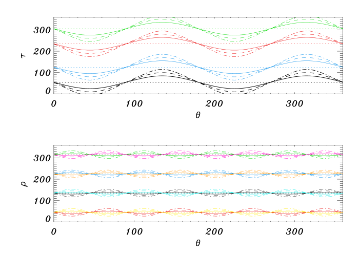
Figure 1.— Retardances of the first (bottom) and second (top) LCVRs as functions of the angle $\theta$ of the etalon orientation with respect to the $S_{2}$ positive direction. Only values between $0$ and $2\pi$ are displayed. Different line types refer to different values of the etalon retardance (see text).

Figure 1 displays the LCVR retardances in $[0,2\pi]$ that guarantee optimum performance as functions of the orientation angle of the etalon. Values for the second LCVR are in the top panel and those for the first one are in the bottom panel. Different colors correspond to different solutions; different line types correspond to different values of the assumed etalon retardance: 0^∘(dotted), 30^∘(solid), 45^∘(dashed), and 60^∘(dashed-dotted). As commented on before, when $\theta_{\rm etalon}=90^{\circ}\/$, both $\rho$ and $\tau$ recover the same value as if the etalon were absent. Moreover, both retardances are periodic with $\theta$, with periods $\pi/4$ ($\rho$) and $\pi/2$ ($\tau$). It is also interesting to note that four out of the eight solutions for $\rho$ are equal to the other four but phase shifted by $\pi/4$.

Now, it is a little tedious but easy to demonstrate that, regardless of how many, mirrors can be introduced in the optical path between the modulator and the analyzer (as in real instruments) without affecting the maximum polarimetric efficiencies, provided they all are perpendicular to the optical axis plane. From the Mueller matrix of a single mirror, one can realize (Collett, 1992) that the matrix of such a mirror train, no matter the angles between them, keeps always the shape

$${\bf E}=\left(\begin{array}[]{cccc}a&b&0&0\\ b&a&0&0\\ 0&0&c&d\\ 0&0&-d&e\end{array}\right).$$ (28)

The elements of the first row in the new final Mueller matrix of the system become $F^{\prime}_{1j}=(a+b)F_{1j}$, $j=1,2,3,4$. That is, the final modulation matrix remains the same as before introducing the mirrors but scaled by a gain factor that can be disregarded as we have been doing for all the treatment. Therefore, we can conclude that optimum efficiencies can still be achieved with as many mirrors as needed. Since a mirror is indeed a combination of a retarder and a partial polarizer (the $d$ element is zero for the latter; see e.g. Stenflo, 1994), the same conclusion can be reached for whatever differential absorption effects for the orthogonal polarization states that may be located between the modulator and the analyzer. Therefore, if, for example, the etalon or the diffraction grating of the instrument display different transmittances for orthogonally polarized beams the polarimetric efficiencies can still attain maximum values.

4. Instrument-induced inaccuracies

Now that we know that our magnetograph can reach optimum polarimetric performance, let us study the behavior of this particular instrument against instabilities in its main optical elements. Photon noise is not the only harm for magnetographic or tachographic measurements. Instabilities of different types like those in the temperature or in the tuning voltage of both the LCVRs and the etalon, or roughness in their final thicknesses, can induce inaccuracies. For single measurements, the inaccuracies can imply errors in magnetic field or absolute wavelength calibration. For time series like those needed in helioseismological studies, such inaccuracies may avoid detection of some particular oscillatory modes. An assessment on such inaccuracies is therefore in order for clearly defining design tolerances of these instrumental quantities. Such tolerances should ensure the fulfillment of the scientific requirements of the instrument.

4.1. Polarimetric inaccuracies

An important example of a scientific requirement is the polarimetric accuracy of the system. By such we understand any of the inverse signal-to-noise ratios for $S_{2}$, $S_{3}$, or $S_{4}$ as defined in Eq. (1). Following our general assumption that these $(S/N)_{i}$ are intended to be the same by design, aiming at a $S/N$ of 1700 is equivalent to require the system to have a polarimetric accuracy of $10^{-3}$. Temperature, voltage, and other instabilities and defects of the LCVRs lead to changes in the retardances that, on their turn, induce modulation and demodulation changes. Such changes can be seen as cross-talk between the Stokes parameters that drive to covariances in the magnetographic measurements (Asensio Ramos & Collados 2008; see also an interesting discussion on seeing-induced cross-talk in Casini et al. 2011). Since our modulation matrix (24) is analytical, we attempt an analytical approach to the study of the effect of these retardance changes onto the polarimetric accuracy of the system.

Let ${\bf D}$ be the demodulation matrix of the instrument that always exists. Thus, ${\bf OD}={\bf DO}={1\mskip-7.0mu1}$. The measured Stokes vector is then given by ${\bf S}={\bf D}{\bf I}_{\rm meas}$, where ${\bf I}_{\rm meas}$ stands for the four intensity measurement vector of each modulation cycle. If we linearly perturb matrix ${\bf D}$ as a consequence of a small perturbation in the LCVR retardances ($\sigma_{\rho_{k}},\sigma_{\tau_{k}},\,k=1,2,3,4$), then the Stokes vector becomes ${\bf S}+{\bf S}^{\prime}=({\bf D}+{\bf D}^{\prime)}{\bf I}_{\rm meas}$, where the perturbed demodulation matrix ${\bf D}^{\prime}$ is given by

$${\bf D}^{\prime}=\sum_{k=1}^{4}\left(\frac{\partial{\bf D}}{\partial\rho_{k}}\sigma_{\rho_{k}}+\frac{\partial{\bf D}}{\partial\tau_{k}}\sigma_{\tau_{k}}\right).$$ (29)

It is obvious that the polarimetric accuracy requirement directly implies that none of the four elements of ${\bf S}^{\prime}={\bf D}^{\prime}{\bf I}_{\rm meas}$ can be greater than $10^{-3}$. To fulfill that requirement, let us then study how the perturbation in the retardances can be produced and which are the tolerances for the instrument quantities whose fluctuations produce them.

If we call $\delta_{L}$ anyone of the retardances, we have by definition that

$$\delta_{L}=\frac{\beta t}{\lambda_{0}},$$ (30)

where $\beta=n_{\rm e}-n_{\rm o}$ is the birefringence, i.e., the difference between the extraordinary and the ordinary refractive indices of the liquid crystal, and $t$ stands for its geometrical thickness. Therefore, it is evident that

$$\frac{\sigma^{2}_{\delta_{L}}}{\delta^{2}_{L}}=\frac{\sigma^{2}_{\beta}}{\beta^{2}}+\frac{\sigma^{2}_{t}}{t^{2}},$$ (31)

that is, the relative inaccuracy in the LCVR retardance is the square root of the sum of the square relative inaccuracies in the birefringence and in the geometrical thickness at the operating wavelength. Let us ascribe for convenience any possible local fabrication defect in the LC like an air bubble to the thickness inaccuracy, so that birefringence can be considered spatially constant for the whole device.

Figure 2.— Retardance (in degree) of a specific nematic LCVR as a function of the acting voltage (in volts; solid line) and its derivative with inverted sign (dashed line).

Variations in the birefringence can be produced by either variations in the LCVR temperature, the acting voltage, or both. Hence, one can write

$$\sigma^{2}_{\beta}=q_{T}^{2}\sigma_{T}^{2}+q_{V}^{2}\sigma_{V}^{2},$$ (32)

where $q_{T}$ and $q_{V}$ are values of the (partial) derivatives of $\beta$ with respect to $T$ and $V$ at the given values of voltage and temperature, respectively. Since we indeed have calibrations of the $\delta_{L}$ dependences rather than those of $\beta$, we better rewrite Eq. (31) as

$$\sigma^{2}_{\delta_{L}}=m_{T}^{2}\,\sigma^{2}_{T}+m_{V}^{2}\,\sigma^{2}_{V}+\frac{\delta_{L}^{2}}{t^{2}}\,\sigma^{2}_{t},$$ (33)

where $m_{T}^{2}$ and $m_{V}^{2}$ have a clear meaning and can be deduced from calibrations. According to Martínez Pillet et al. (2011), based on data by Heredero et al. (2007),

$$m_{T}=-1.16+0.305V-0.02V^{2},$$ (34)

for $V<8$ volt and $0$ otherwise, and $m_{V}$ can be obtained from data like those displayed in Fig. 2 where $\delta_{L}$ (solid line) and its derivative (dashed line; inverted sign) are plotted as functions of the acting voltage for a particular LCVR.

To get a numerical estimation of the value of real tolerances, that is, of the maximum $\sigma_{T}$, $\sigma_{V}$, and $\sigma_{t}$ affordable in real instruments in order not to have the ${\bf S}^{\prime}$-elements greater than $10^{-3}$, we shall use IMaX parameters plus the analytic expressions for ${\bf D}$ and its partial derivatives. The last term in Eq. (33) may vary spatially and is, thus, responsible for the pixel-to-pixel variations of the retardance but can easily be calibrated if needed. Indeed, roughness in the device thickness is a fabrication specification and can be checked upon delivery from the manufacturer. Thickness inaccuracies may produce locally significant effects (e.g., Alvarez-Herrero et al., 2010). Our own estimation, using Eqs. (29, 33) indicate that relative errors in the thickness larger than 6 % induce perturbations of the Stokes vector that are larger than the polarimetric accuracy. Therefore, should this be the only instrumental instability, specific pixel-to-pixel calibration of ${\bf D}$ would be needed if the relative roughness is larger than 6 %. Note that, since the typical thicknesses of LCVRs are of the order of micrometers, a roughness less than 6% may mean a stringent requirement for the manufacturer of the order of tens of nanometers.

Using again Eqs. (29, 33), we find out that instabilities larger than $\sigma_{T}=600$ mK or $\sigma_{V}=1.5$ mV deteriorate the polarimetric accuracy below the required $10^{-3}$. These two tolerances and that for the roughness have been calculated after assuming that each instability is acting individually. According to Eq. (33), the final uncertainty in the retardance stems from the three sources simultaneously. Hence, a safety reduction factor of $\sqrt{3}$ (assuming all the three contribute the same) is advisable. Therefore, in the end, the final tolerance specification for our instrument to reach a polarimetric accuracy of $10^{-3}$ is 300 mK for temperature, 1 mV for voltage, and a 4 % for LCVR roughness.

4.2. Magnetographic inaccuracies

The retardance perturbations of Eq. (33) induce changes in the maximum polarimetric efficiencies of the instrument. Such changes necessarily imply modifications in the magnetographic measurements. The modifications might jeopardize the quality of the results. Imagine, for instance, that a requirement on the repeatability of $B_{\rm lon}$ and $B_{\rm tran}$ applies because we are interested on a measurement time series: a calculation of tolerances in the instrument parameters ($T$, $V$, roughness, etc.) that ensure the fulfillment of the magnetographic repeatability is in order.

Since no explicit dependence of $B_{\rm lon}$ and $B_{\rm tran}$ on $\varepsilon_{i}$ exists, we cannot analytically gauge the induced inaccuracies in any magnetographic measurement. Nevertheless, we can obtain a hint on the global by studying the specific variations of $\delta(B_{\rm lon})$ and $\delta(B_{\rm tran})$, the minimum detectable values of such magnetograph quantities.

Error propagation in Eqs. (15) and (16) readily gives

$$\sigma^{2}_{{\delta(B_{\rm lon})}}=\frac{{\delta^{2}(B_{\rm lon})}}{4\varepsilon_{4}^{2}}\,\sigma^{2}_{\varepsilon^{2}_{4}}$$ (35)

and

$$\sigma^{2}_{{\delta(B_{\rm tran})}}=\frac{{\delta^{2}(B_{\rm tran})}}{16\varepsilon_{2}^{2}}\,\sigma^{2}_{\varepsilon^{2}_{2}}=\frac{{\delta^{2}(B_{\rm tran})}}{16\varepsilon_{3}^{2}}\,\sigma^{2}_{\varepsilon^{2}_{3}}.$$ (36)

According to Del Toro Iniesta & Collados (2000), the maximum polarimetric efficiencies that can be reached by any system are

$$\varepsilon^{2}_{{\rm max},i}=\frac{\sum_{j=1}^{4}O^{2}_{ji}}{N_{p}},$$ (37)

where $O_{ji}$ are the matrix elements of ${\bf O}^{\rm T}$, the transpose of $\bf O$. For a system with a modulation matrix like that in Eq. (24), it is easy to see that the efficiency inaccuracies ensuing the thermal instabilities are

$$\sigma^{2}_{\varepsilon^{2}_{{\rm max},1}}=0,$$ (38)

as a consequence of using normalized Mueller matrices, and

$$\sigma^{2}_{\varepsilon^{2}_{{\rm max},2}}=\frac{1}{16}\sum_{j=1}^{4}\sin^{2}2\tau_{j}\,\,\sigma^{2}_{\tau_{j}},$$ (39)

$$\sigma^{2}_{\varepsilon^{2}_{{\rm max},3}} = \frac{1}{16}\left\{\sum_{j=1}^{4}\sin^{2}2\rho_{j}\,\,\sin^{4}\tau_{j}\,\,\sigma^{2}_{\rho_{j}}\right.+$$ (40)

$$\left.\sum_{j=1}^{4}\sin^{4}\rho_{j}\,\,\sin^{2}2\tau_{j}\,\,\sigma^{2}_{\tau_{j}}\right\},$$

$$\sigma^{2}_{\varepsilon^{2}_{{\rm max},4}} = \frac{1}{16}\left\{\sum_{j=1}^{4}\sin^{2}2\rho_{j}\,\,\sin^{4}\tau_{j}\,\,\sigma^{2}_{\rho_{j}}\right.+$$ (41)

$$\left.\sum_{j=1}^{4}\cos^{4}\rho_{j}\,\,\sin^{2}2\tau_{j}\,\,\sigma^{2}_{\tau_{j}}\right\},$$

where $\sigma^{2}_{\tau_{j}}$ and $\sigma^{2}_{\rho_{j}}$ are the variances of the LCVR retardances and where we have neglected the influence of possible time-exposure differences or instabilities like those caused by a rolling-shutter detector or a non-ideal repeatability of a mechanical shutter. Such influences can be estimated separately for the specific instrument and directly scale the effective exposure time (either per pixel or per frame).

Using the values for IMaX, and assuming maximum efficiencies, instabilities of 0.3 K or of 1.1 mV produce a 5 % repeatability error in the threshold for $B_{\rm lon}$. A comparison of Eqs. (35) and (36) readily tells that the effect is 2 times smaller on the relative repeatability error in the threshold for $B_{\rm tran}$ but since the threshold itself is 16 times larger, the absolute error is in the end 8 times larger as well.

4.3. Velocity inaccuracies

Error propagation in Eq. (17) yields

$$\sigma_{v_{\rm LOS}}^{2}=\left(\frac{\partial v_{\rm LOS}}{\partial\delta\lambda}\right)^{2}\sigma_{\delta\lambda}^{2}+\left(\frac{\partial v_{\rm LOS}}{\partial\lambda_{0}}\right)^{2}\sigma_{\lambda_{0}}^{2}+\sum_{k}\left(\frac{\partial v_{\rm LOS}}{\partial S_{1,k}}\right)^{2}\sigma_{{1,k}}^{2}$$ (42)

with $k=-9,-3,+3,+9$. Uncertainties in the spectral resolution come from uncertainties in the etalon spacing and related fabrication details that produce etalon roughness. Errors in the central wavelength come from the etalon tuning that mostly depends on the ambient temperature, $T$, and on the tuning voltage, $V$:

$$\sigma_{\lambda_{0}}^{2}=k_{T}^{2}\sigma_{T}^{2}+k_{V}^{2}\sigma_{V}^{2},$$ (43)

where $k_{T}$ and $k_{V}$ are constants that give the (linear) dependence of $\lambda_{0}$ on $T$ and $V$. Finally, uncertainties in the Stokes $S_{1}$ samples come both from pure photon noise, as in any photometric measurement, and from etalon tuning uncertainties. Since the (inexplicit) dependence of $S_{1,k}$ on $\lambda_{0}$ is non linear, let us linearize it (that is, introduce a small perturbation and take the first approximation) and write

$$\sigma_{1,k}^{2}=\sigma_{1}^{2}+s_{1,k}^{2}\sigma_{\lambda_{0}}^{2},$$ (44)

where we have assumed that the photometric contribution is equal for all the samples and indeed equal to the photon noise as calculated in the continuum; $s_{1,k}$ stand for the derivatives of the Stokes $S_{1}$ profile at the corresponding wavelengths.

After a tedious but straightforward algebra, Eq. (42) can be recast as

$$\sigma_{v_{\rm LOS}}^{2}=\frac{v_{\rm LOS}^{2}}{(\delta\lambda)^{2}}\sigma_{\delta\lambda}^{2}+\frac{4c^{2}(\delta\lambda)^{2}}{\pi^{2}\lambda_{0}^{2}}\frac{2\sigma_{1}^{2}}{\Delta}+$$

$$\left[\frac{v_{\rm LOS}^{2}}{\lambda_{0}^{2}}+\frac{4c^{2}(\delta\lambda)^{2}}{\pi^{2}\lambda_{0}^{2}}\frac{d_{1}+d_{2}}{\Delta^{2}}\right](k_{T}^{2}\sigma_{T}^{2}+k_{V}^{2}\sigma_{V}^{2}),$$ (45)

where $\Delta$ is defined in Sect. 2.1, $d_{1}=(S_{1,+9}-S_{1,-3})^{2}(s_{1,-9}^{2}+s_{1,+3}^{2})$ and $d_{2}=(S_{1,-9}-S_{1,+3})^{2}(s_{1,+9}^{2}+s_{1,-3}^{2})$. Hence, clear contributions to the final LOS velocity uncertainty can be discerned from the etalon roughness, the photon noise, the etalon temperature instability, and the etalon voltage instability.

Quantitative estimates of the various terms in Eq. (45) can be made by using the FTS spectrum by Brault & Neckel (1987) to evaluate $\Delta$, $d_{1}$, and $d_{2}$ for a given spectral line and a given instrument. Let assume the HMI and SO/PHI Fe i line at $\lambda_{0}=617.3$ nm and a spectral resolution of the etalon of $\delta\lambda=10$ pm. The first term has a clear impact on the tachographic results: the etalon relative roughness is directly translated into the same $v_{\rm LOS}$ relative uncertainty. In other words, we cannot expect better accuracy in the line-of-sight velocity (when measured with the Fourier tachometer formula) than that limited by the etalon relative roughness; this means that a mere 0.1 pm, rms resolution uncertainty induces 10 m s^-1 errors for speeds of 1 km s^-1. The second term coincides with the right-hand side of Eq. (23) and has been discussed already in Sect. 2.1. Since the ratio between the second and the first terms within brackets is of the order of 4$\cdot$10⁹ for velocities of up to 5 km s^-1, it is the second one what really matters in the estimation; this means that the dependence of the profile shape on the central wavelength of the line is really important. If we use the same IMaX values of $k_{T}=2.52$ pm/K and $k_{V}=3.35\cdot$10^-2 pm/V for the SO/PHI etalon, Eq. (45) gives instabilities of the order of 3.3 mK or 0.25 V induce the same LOS velocity uncertainty of 4 km s^-1 quoted above for pure photon noise. Another way of seeing the same effect can be explained by saying that a 100 m s^-1 uncertainty is produced by either a 45 mK or a 3.4 V instabilities. These uncertainties are really important when stability during given periods of time of the instrument is required as for helioseismic measurements. For single shots, uncertainties in temperature or voltage imply thresholds for accurate absolute wavelength (velocity) calibration. The importance of having included the measurement technique in this error budget analysis is clear: should one have simply used the $k_{V}$ and $k_{T}$ calibration constants above and the Doppler formula an uncertainty of just 55 m s^-1 would have been obtained. Hence, the uncertainty would have been underestimated by a factor almost 2.

5. Summary and conclusions

An assessment study on the salient features and properties of solar magnetographs has been presented. An error budget procedure has been followed. Special care has been devoted in including photon-induced and instrument-induced noise as well as specific measurement technique contributions to the final variances. We have first discussed the effect of random noise in the measurements and deduced useful formulae –general for every device– that provide some minimum detectable parameters like the degree of polarization of light, the longitudinal and transverse components of the magnetic field, and the line-of-sight velocity. The detection thresholds are given as functions of the polarimetric efficiencies of the instrument and of the signal-to-noise ratio of the observations. (As a proposal, we have suggested as well to use the $S/N$ for the Stokes intensity as the signal-to-noise ratio for the instrument.) When the random noise is photon-induced, we have calculated as well the relative uncertainty in the magnetographic and tachographic quantities. Secondly, an analysis is presented for those instruments based on two nematic liquid crystal variable retarders as a polarization modulator and a Fabry-Pérot etalon as the spectrum analyzer. Although specific for these magnetographs, the methodology can easily be followed by others in order to characterize their capabilities and accuracies. We have demonstrated that this type of instrument can indeed reach theoretical maximum polarimetric efficiencies because solutions always exist for the retardances of the two LCVRs that ensure such efficiencies, hence optimizing the detection thresholds and the relative uncertainties. Very remarkably, the existence of such solutions is independent of the optics that is in between the polarization modulator and the analyzer. Neither retarders nor partial polarizers or mirrors (the most commonly used devices) alter that property. The LCVR optimum retardances do depend in such pass-through optics but can be fine-tuned according to the polarizing properties of the optics. A number of rules and periodicity properties of the required retardances have also been deduced. These polarimeters have modulation and demodulation matrices that are explicitly calculated through an IDL procedure that is available upon request. Thirdly, error propagation has yielded equations relating the variances of the measured Stokes vector and the solar physical quantities and instrument parameters, hence providing a bridge between scientific requirements and instrument design specifications. The analytic character of this particular type of instrument has also allowed the quantitative estimation of the mentioned uncertainties. Hopefully, the discussion presented in this paper excites (and helps) further diagnostics of other instruments.

References

- Alvarez-Herrero et al. (2010) Alvarez-Herrero, A., Martínez-Pillet, V., Del Toro Iniesta, J. C., Domingo, V., & the IMaX team. 2010, in API’09 - First NanoCharM Workshop on Advanced Polarimetric Instrumentation, EPJ Web of Conferences, ed. E. García-Caurel & A. de Martino, Vol. 5, 5002
- Asensio Ramos & Collados (2008) Asensio Ramos, A. & Collados, M. 2008, Appl. Opt., 47, 2541
- Barthol et al. (2011) Barthol, P., Gandorfer, A., Solanki, S. K., Schüssler, M., Chares, B., Curdt, W., Deutsch, W., Feller, A., Germerott, D., Grauf, B., Heerlein, K., Hirzberger, J., Kolleck, M., Meller, R., Müller, R., Riethmüller, T. L., Tomasch, G., Knölker, M., Lites, B. W., Card, G., Elmore, D., Fox, J., Lecinski, A., Nelson, P., Summers, R., Watt, A., Martínez Pillet, V., Bonet, J. A., Schmidt, W., Berkefeld, T., Title, A. M., Domingo, V., Gasent Blesa, J. L., Del Toro Iniesta, J. C., López Jiménez, A., Álvarez-Herrero, A., Sabau-Graziati, L., Widani, C., Haberler, P., Härtel, K., Kampf, D., Levin, T., Pérez Grande, I., Sanz-Andrés, A., & Schmidt, E. 2011, Sol. Phys., 268, 1
- Beck et al. (2010) Beck, C., Bellot Rubio, L. R., Kentischer, T. J., Tritschler, A., & Del Toro Iniesta, J. C. 2010, A&A, 520, A115
- Beckers & Brown (1978) Beckers, J. & Brown, T. 1978, in Future solar optical observations. Needs and contraints, ed. G. Godoli, Vol. 106, 189
- Brault & Neckel (1987) Brault, J. W. & Neckel, H. 1987, Spectral atlas of solar absolute disk averaged and disk-center intensity from 3290 to 12510Å, Tech. rep., Hamburg University, Hamburg
- Brown (1981) Brown, T. 1981, in Solar instrumentation: What’s next?, ed. R. B. Dunn, 150
- Cabrera Solana et al. (2005) Cabrera Solana, D., Bellot Rubio, L. R., & Del Toro Iniesta, J. C. 2005, A&A, 439, 687
- Casini et al. (2011) Casini, R., de Wijn, A. G., & Judge, P. G. 2011, ArXiv e-prints
- Collados et al. (2007) Collados, M., Lagg, A., Díaz García, J. J., Hernández Suárez, E., López López, R., Páez Mañá, E., & Solanki, S. K. 2007, in ASP Conference Series, Vol. 368, The Physics of Chromospheric Plasmas, ed. P. Heinzel, I. Dorotovič, & R. J. Rutten, 611
- Collett (1992) Collett, E. 1992, Polarized light. Fundamentals and applications (Optical Engineering, New York: Dekker)
- Del Toro Iniesta (2003) Del Toro Iniesta, J. C. 2003, Introduction to Spectropolarimetry (Cambridge, UK: Cambridge University Press)
- Del Toro Iniesta & Collados (2000) Del Toro Iniesta, J. C. & Collados, M. 2000, Appl. Opt., 39, 1637
- Del Toro Iniesta & Martínez Pillet (2010) Del Toro Iniesta, J. C. & Martínez Pillet, V. 2010, ArXiv e-prints
- Del Toro Iniesta & Orozco Suárez (2010) Del Toro Iniesta, J. C. & Orozco Suárez, D. 2010, Astronomische Nachrichten, 331, 558
- Del Toro Iniesta et al. (2010) Del Toro Iniesta, J. C., Orozco Suárez, D., & Bellot Rubio, L. R. 2010, ApJ, 711, 312
- Del Toro Iniesta & Ruiz Cobo (1996) Del Toro Iniesta, J. C. & Ruiz Cobo, B. 1996, Sol. Phys., 164, 169
- Fernandes (1992) Fernandes, D. N. 1992, PhD thesis, Stanford Univ., CA.
- Graham et al. (2003) Graham, J. D., Norton, A., López Ariste, A., Lites, B., Socas-Navarro, H., & Tomczyk, S. 2003, in Astronomical Society of the Pacific Conference Series, Vol. 307, Third International Workshop on Solar Polarization, ed. J. Trujillo-Bueno & J. Sánchez Almeida, 131
- Heredero et al. (2007) Heredero, R. L., Uribe-Patarroyo, N., Belenguer, T., Ramos, G., Sánchez, A., Reina, M., Martínez Pillet, V., & Álvarez-Herrero, A. 2007, Appl. Opt., 46, 689
- Keller & Snik (2009) Keller, C. U. & Snik, F. 2009, in Astronomical Society of the Pacific Conference Series, Vol. 405, Solar Polarization 5: In Honor of Jan Stenflo, ed. S. V. Berdyugina, K. N. Nagendra, & R. Ramelli, 371
- Kosugi et al. (2007) Kosugi, T., Matsuzaki, K., Sakao, T., Shimizu, T., Sone, Y., Tachikawa, S., Hashimoto, T., Minesugi, K., Ohnishi, A., Yamada, T., Tsuneta, S., Hara, H., Ichimoto, K., Suematsu, Y., Shimojo, M., Watanabe, T., Shimada, S., Davis, J. M., Hill, L. D., Owens, J. K., Title, A. M., Culhane, J. L., Harra, L. K., Doschek, G. A., & Golub, L. 2007, Sol. Phys., 243, 3
- Landi Degl’Innocenti & Landi Degl’Innocenti (1977) Landi Degl’Innocenti, E. & Landi Degl’Innocenti, M. 1977, A&A, 56, 111
- Lites et al. (2001) Lites, B. W., Elmore, D. F., & Streander, K. V. 2001, in Astronomical Society of the Pacific Conference Series, Vol. 236, Advanced Solar Polarimetry – Theory, Observation, and Instrumentation, ed. M. Sigwarth, 33
- Marsch et al. (2005) Marsch, E., Marsden, R., Harrison, R., Wimmer-Schweingruber, R., & Fleck, B. 2005, Advances in Space Research, 36, 1360
- Martínez Pillet (2007) Martínez Pillet, V. 2007, in Proc. of the Second Solar Orbiter Workshop, SP-641, ESA (ESA)
- Martínez Pillet et al. (2004) Martínez Pillet, V., Bonet, J. A., Collados, M. V., Jochum, L., Mathew, S., Medina Trujillo, J. L., Ruiz Cobo, B., Del Toro Iniesta, J. C., López Jimenez, A. C., Castillo Lorenzo, J., Herranz, M., Jeronimo, J. M., Mellado, P., Morales, R., Rodriguéz, J., Alvarez-Herrero, A., Belenguer, T., Heredero, R. L., Menendez, M., Ramos, G., Reina, M., Pastor, C., Sánchez, A., Villanueva, J., Domingo, V., Gasent, J. L., & Rodriguéz, P. 2004, in Society of Photo-Optical Instrumentation Engineers (SPIE) Conference Series, Vol. 5487, Society of Photo-Optical Instrumentation Engineers (SPIE) Conference Series, ed. J. C. Mather, 1152–1164
- Martínez Pillet et al. (1999) Martínez Pillet, V., Collados, M., Sánchez Almeida, J., González, V., Cruz-López, A., Manescau, A., Joven, E., Páez, E., Díaz, J., Feeney, O., Sánchez, V., Scharmer, G., & Soltau, D. 1999, in ASP Conf. Series, 183, 264
- Martínez Pillet et al. (2011) Martínez Pillet, V., Del Toro Iniesta, J. C., Alvarez-Herrero, A., Domingo, V., Bonet, J. A., Gonzalez Fernandez, L., Lopez Jimenez, A., Pastor, C., Gasent Blesa, J. L., Mellado, P., Piqueras, J., Aparicio, B., Balaguer, M., Ballesteros, E., Belenguer, T., Bellot Rubio, L. R., Berkefeld, T., Collados, M., Deutsch, W., Feller, A., Girela, F., Grauf, B., Heredero, R. L., Herranz, M., Jeronimo, J. M., Laguna, H., Meller, R., Menendez, M., Morales, R., Orozco Suarez, D., Ramos, G., Reina, M., Ramos, J. L., Rodriguez, P., Sanchez, A., Uribe-Patarroyo, N., Barthol, P., Gandorfer, A., Knoelker, M., Schmidt, W., Solanki, S. K., & Vargas Dominguez, S. 2011, Sol. Phys., 268, 57
- Mein (1971) Mein, P. 1971, Sol. Phys., 20, 3
- Narayan et al. (2008) Narayan, G., Scharmer, G. B., Hillberg, T., Lofdahl, M., van Noort, M., Sutterlin, P., & Lagg, A. 2008, in 12th European Solar Physics Meeting, Freiburg, Germany
- Orozco Suárez & Del Toro Iniesta (2007) Orozco Suárez, D. & Del Toro Iniesta, J. C. 2007, A&A, 462, 1137
- Ruiz Cobo & Del Toro Iniesta (1994) Ruiz Cobo, B. & Del Toro Iniesta, J. C. 1994, A&A, 283, 129
- Sankarasubramanian et al. (2003) Sankarasubramanian, K., Elmore, D. F., Lites, B. W., Sigwarth, M., Rimmele, T. R., Hegwer, S. L., Gregory, S., Streander, K. V., Wilkins, L. M., Richards, K., & Berst, C. 2003, in SPIE Conference Series, ed. S. Fineschi, Vol. 4843, 414–424
- Scharmer et al. (2008) Scharmer, G. B., Narayan, G., Hillberg, T., de la Cruz Rodriguez, J., Löfdahl, M. G., Kiselman, D., Sütterlin, P., van Noort, M., & Lagg, A. 2008, ApJ, 689, L69
- Stenflo (1994) Stenflo, J. O. 1994, Astrophysics and Space Science Library, Vol. 189, Solar magnetic fields (Dordrecht, The Netherlands: Kluwer Academic Publishers)
- Title (2000) Title, A. 2000, in Bulletin of the American Astronomical Society, Vol. 32, AAS/Solar Physics Division Meeting #31, 839