Simplified Pair Copula Constructions — Limits and Extensions

Abstract

So called pair copula constructions (PCCs), specifying multivariate distributions only in terms of bivariate building blocks (pair copulas), constitute a flexible class of dependence models. To keep them tractable for inference and model selection, the simplifying assumption that copulas of conditional distributions do not depend on the values of the variables which they are conditioned on is popular. In this paper, we show for which classes of distributions such a simplification is applicable, significantly extending the discussion of haff2010b. In particular, we show that the only Archimedean copula in dimension $d\geq 4$ which is of the simplified type is that based on the gamma Laplace transform or its extension, while the Student-t copula is the only one arising from a scale mixture of Normals. Further, we illustrate how PCCs can be adapted for situations where conditional copulas depend on values which are conditioned on.

Keywords: archimedean copula; elliptical copula; pair copula construction; conditional distribution

1 Introduction

Growing capabilities to store large data sets and increasing computing power for their computational analysis substantially increased the demand to develop statistical methodology for many dependent variables over the last years. The properties of high-dimensional distributions in general, however, remain hard to understand intuitively. Given that, the early focus was on the multivariate Normal distribution, which allows to describe the whole dependence structure by specifying bivariate correlations. These linear dependencies between just two variables remain easy to understand and communicate. But more recent developments, in particular in econometrics (c.f. longin2001, ang2002b), showed that many data sets in higher dimensions exhibit more complex dependence structures.

To deal with these challenging structures and keeping the model understandable at the same time, a popular technique is to sequentially decompose the joint distributions into bivariate building blocks by conditioning. These are then modeled using bivariate copulas of which many parametric families are well studied, see for example the monographs by Joe and Nelsen. Distributions arising from such a decomposition are called pair copula constructions (PCCs). The question for which classes of multivariate models and under which assumptions such a sequential conditioning is possible, however, remained unsolved. The only publication in this direction is haff2010b, providing first illustrative examples.

In this paper, we fill in this gap by classifying multivariate distributions in terms of the dependence properties of their conditional distributions (see Figure 1). Special attention will be paid to the simplifying assumption that the copulas corresponding to conditional distributions are constant irrespective of the values of variables that they are conditioned on. This assumption is usually made to keep model selection and inference tractable, and we will show for which multivariate distributions it holds. Furthermore, we discuss how constructions based on simplified PCCs can be extended when the simplifying assumption is not applicable.

The remainder is structured as follows. Section 2 introduces PCCs. In Section 3 and 4, we demonstrate which Archimedean and elliptical copulas are simplified PCCs. Section 5 provides the remaining examples for the classification in Figure 1 and considers the increased flexibility gained by weakening the simplifying assumption. Section 6 concludes with an outlook to areas of future research.

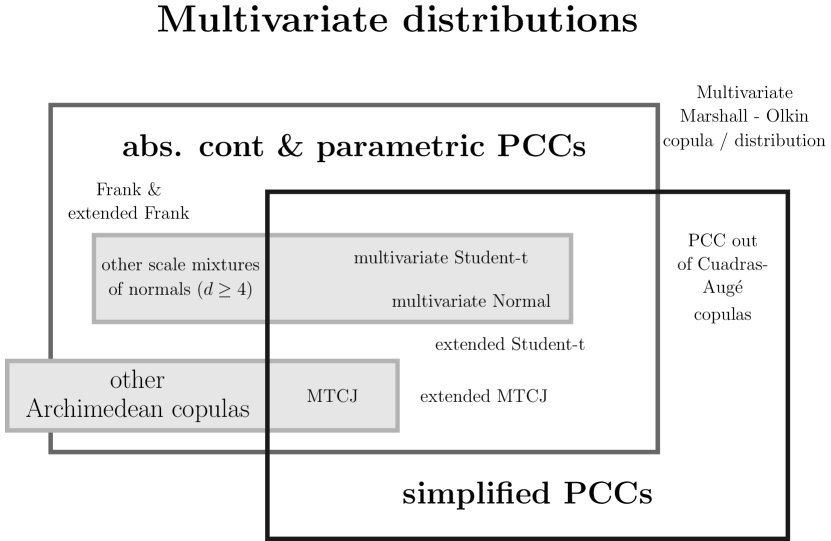
Figure 1: Overview of the PCC classes which are discussed including their relations and examples.

2 Pair copula constructions

A copula is defined as the cumulative distribution function (cdf) of a multivariate distribution with uniform$(0,1)$ margins. These have become of great importance in multidimensional dependence modeling, since the theorem of sklar allows to separate the specification of a $d$-dimensional distribution $F$ into specifying the univariate marginal distribution functions $F_{i}$, $i=1,\ldots,d$, and a copula $C$, i.e., to find $C$ such that

$$F_{1:d}(x_{1},\ldots,x_{d})=C_{1:d}(F_{1}(x_{1}),\ldots,F_{d}(x_{d})).$$

Here, we use the abbreviation $i:j:=(i,i+1,\ldots,j)$ for $i<j$. In particular bivariate copula families are well studied, and every multivariate distributions can be constructed from marginal distributions and two-dimensional copulas by sequential conditioning, a so-called pair-copula construction. While different principles for PCCs such as regular vines (R-vines) (bedford2001 2001; 2002) or non-Gaussian directed acyclic graphs (DAGs) Bauer et al. (2011) have been investigated over the years, the underlying basic idea is always that of Joe (1996):

Let us consider three random variables (rvs) $X_{1}$, $X_{2}$ and $X_{3}$ with corresponding cumulative distribution functions (cdfs) $F_{1},F_{2}$ and $F_{3}$, then we can first construct a joint distribution of $(X_{1},X_{2})$ and of $(X_{3},X_{2})$ by assigning copula functions $C_{12}$ and $C_{32}$, respectively:

$$\begin{split}F_{12}(x_{1},x_{2})&:=C_{12}\left(F_{1}(x_{1}),F_{2}(x_{2})\right)\\ F_{32}(x_{3},x_{2})&:=C_{32}\left(F_{1}(x_{3}),F_{2}(x_{2})\right)\\ \end{split}$$ (1)

These bivariate distributions can be combined to a three-dimensional distribution by assigning a conditional copula $C_{13|2}$,

$$F_{123}(x_{1},x_{2},x_{3}):=\int_{-\infty}^{\infty}C_{13|2}(F_{1|2}(x_{1}|x_{2}),F_{3|2}(x_{3}|x_{2});x_{2})\ dF_{2}(x_{2}).$$ (2)

For every cdf $F_{123}$, Sklar’s theorem implies the existence of a bivariate copula that couples $F_{1|2}(\cdot|x_{2})$ and $F_{3|2}(\cdot|x_{2})$ for every $x_{2}$. The generalization of this principle to arbitrary dimensions is obvious and the conditional copulas corresponding to such a construction can be determined for every multivariate distribution (c.f. Patton (2006) for a discussion of conditional copulas).

To make PCCs tractable for inference and model selection however, further assumptions regarding the conditional copulas have to be made.
We will call a multivariate distribution an absolutely continuous and parametric PCC if all bivariate copula families occurring in the construction have densities with a parameter vector. In this case, it will be possible to express the likelihood function of the joint copula model in terms of the bivariate densities and to make inference about the finite-dimensional parameter based on this expression. One example for this would be the decomposition of a $d$-dimensional density $f$ with marginal densities $f_{k}$, $1\leq k\leq d$, as a C-vine copula (see aas2009): with univariate parameters $\theta_{k}$ and copula parameters $\theta_{j,j+i}$, and $\mbox{\boldmath$\theta$}=(\theta_{1},\ldots,\theta_{d};\theta_{j,j+i},j=1,\dots,d-1,i=1,\dots,d-j)$,

$$\begin{split}f_{1:d}(x_{1},&\dots,x_{d};\mbox{\boldmath$\theta$})=\prod_{k=1}^{d}f_{k}(x_{k};\theta_{k})\ \cdot\\ &\prod_{j=1}^{d-1}\prod_{i=1}^{d-j}c_{j,j+i|1:(j-1)}\left(F_{j|1:(j-1)}(x_{j}|\textbf{x}_{1:(j-1)}),F_{j+i|1:(j-1)}(x_{j+i}|\textbf{x}_{1:(j-1)});\theta_{j,j+i}\right).\end{split}$$

The above multivariate density is valid for a simplified PCC because all bivariate copulas occurring in the constructions do not depend on the variables that are conditioned on, e.g.,

$$C_{13|2}(\cdot,\cdot;x_{2})=C_{13|2}(\cdot,\cdot).$$

This simplifying assumption reduces the specification of a PCC to choosing bivariate copula families and their parameters. This means that the potentially complex dependence between variables that are conditioned on and the copula functions can be neglected, and model selection can be performed more easily. Also other techniques for PCCs such as for R-vines (stepwise estimation in Hobæk Haff (2012) and dissmann2011, inference as in aas2009 or Bayesian techniques as in Min and Czado (2010)) extend to the non-simplified case only if the dependence on the variables that are conditioned on is of a simple form (we discuss this in Section 5, see in particular Example 5.1).

3 Archimedean copulas

In this section, we characterize the Archimedean copulas that are simplified PCCs. A $d$-dimensional Archimedean copula is given by

$$C_{1:d}(u_{1},\dots,u_{d})=\varphi\Big{(}\sum_{j=1}^{d}\varphi^{-1}(u_{j})\Big{)},$$ (3)

for an Archimedean generator function $\varphi\in\mathcal{L}_{d}$. Here, $\mathcal{L}_{d}$ is the class of functions $\varphi:[0,\infty)\mapsto[0,1]$, which are strictly decreasing on $[0,\inf\{s,\varphi(s)=0\}]$ (with $\varphi(0)=1$, $\varphi(\infty)=0$) and differentiable on $[0,\infty)$ up to order $d-2$, such that $(-1)^{j}\varphi^{(j)}\geq 0,j=1,\dots,d-2$, and where further $(-1)^{d-2}\varphi^{(d-2)}$ is non-increasing and convex (McNeil and Nešlehová (2009), Joe (1997), Müller and Scarsini (2005)). These copulas have the appealing property that the conditional distribution function is given in a simple analytical form which facilitates the study of their properties. Given a Gamma random variable with shape parameter $p$, rate parameter $b$, density

$$f_{\Gamma}(x;b,p)=\frac{b^{p}}{\Gamma(p)}x^{p-1}e^{-bx},$$

mean $p/b$ and variance $p/b^{2}$, the Laplace transform (LT) is

$$\varphi_{\Gamma}(s;\theta)=\int_{0}^{\infty}e^{-sx}f_{\Gamma}(x;1/\theta,1/\theta)dx=(1+\theta s)^{-1/\theta},\ \ \theta\geq 0.$$

The Archimedean copula corresponding to this LT as generator function is called MTCJ copula. From the form of the conditional distributions derived in Takahasi (1965) it is obvious that the copulas corresponding to bivariate conditional margins of the MTCJ copula are again MTCJ copulas. The above gamma LT family extends to Archimedean generators (for the generalized MTCJ family)

$$\varphi_{\Gamma}(s;\theta)=\left(1+\theta\cdot s\right)_{+}^{-1/\theta},\ \ \theta\geq-\frac{1}{d-1},\ \ (x)_{+}=\max\{0,x\}.$$ (4)

The conditional generator (c.f. Mesfioui and Quessy (2008)) when conditioning on $m$ variables becomes

$$\varphi_{m}(s;\theta)=\left(1+\frac{s\theta}{m\theta+1}\right)_{+}^{-(m\theta+1)/\theta}.$$ (5)

For $\theta\geq 1/(d-1)$, $\theta/(m\theta+1)\geq 1/(d-1-m)$, so the parameter range is consistent, and the (generalized) MTCJ copula is a simplified PCC where all bivariate building blocks are MTCJ with corresponding choice of parameters. In fact, under a weak regularity assumption, it is the only multivariate Archimedean copula that constitutes a simplified PCC.

Theorem 3.1

A $d$-dimensional Archimedean copula with a generator that is twice continuously differentiable on the set where it is positive is a simplified PCC if and only if its generator is in the family (4).

Proof

Appendix A. $\Box$

Note that the differentiability condition for the generator is satisfied for all Archimedean copulas if $d\geq 4$. This adds a further aspect making the MTCJ copula unique among Archimedean copulas. Using different parameters than obtained through Equation (5), PCCs with MTCJ copulas with freely chosen parameters as building blocks naturally generalize the MTCJ copula to what we call an extended MTCJ copula.

4 Elliptical copulas

In this section, we characterize the elliptical copulas that have all conditional distributions in location-scale families. We show that not all elliptical copulas are simplified PCCs and characterize the scale mixtures of Normals which are of the simplified type. By referring to a $d$-dimensional elliptical copula we mean a copula arising from an elliptical distribution such as the multivariate Normal or Student-$t$ distribution. A multivariate distribution is elliptical if its characteristic function has the form

$$\text{\textphi}_{\textbf{X}}(\textbf{t};\bm{\mu},\Sigma)=\Psi(\textbf{t}^{\prime}\Sigma\textbf{t})e^{i\textbf{t}^{\prime}{\bm{\mu}}},$$

for $\Psi:\mathbb{R}_{0}^{+}\mapsto\mathbb{R}$, $\mbox{\boldmath$\mu$}\in\mathbb{R}^{d}$, and positive definite $\Sigma\in\mathbb{R}^{d\times d}$. If the distribution has a density, this implies that it is given by

$$f_{\textbf{X}}(\textbf{x})=\lvert\Sigma\rvert^{-1/2}g\Big{(}(\textbf{x}-\mbox{\boldmath$\mu$})^{\prime}\Sigma^{-1}(\textbf{x}-\mbox{\boldmath$\mu$})\Big{)},$$

for a generator function $g:\mathbb{R}^{+}_{0}\mapsto\mathbb{R}^{+}_{0}$, which can be uniquely determined from $\Psi$, see cambanis1981. For the two examples we mentioned, the generator functions have the form

$$g_{\text{Gauss},n}(t)=\frac{1}{(2\pi)^{n/2}}e^{-t/2},\ \ \ g_{\text{Student}-t,n,\nu}(t)=\frac{\Gamma\left(\frac{\nu+n}{2}\right)}{\Gamma\left(\frac{\nu}{2}\right)(\nu\pi)^{n/2}}\cdot\left(1+\frac{t}{\nu}\right)^{-\left(\nu+n\right)/2},$$

and lead to simplified PCCs.

Theorem 4.1

The multivariate Gaussian distribution and the multivariate Student-$t$ distribution are PCCs of the simplified form.

For the Gaussian distribution this is quite obvious since all conditional distributions are again Gaussian and do depend on the values of the variables that they are conditioned on only through their mean, i.e., they all are in the same location family. For the Student-$t$ distribution the covariances also depend on these values, but only through a scaling factor such that all conditional distributions remain in the same location-scale family. Since changes of location and scale do not affect the copula of a multivariate distribution, this implies that the Student-$t$ distribution is a simplified PCC. For clarification, we derive the explicit form of the copulas corresponding to bivariate conditional distributions in Appendix B.1. Just as for the MTCJ copula, changing the degrees of freedom in the bivariate building blocks of the PCC leads to a natural extension of the multivariate Student-t distribution in which different bivariate conditional margins can have different degrees of freedom.

While the copulas corresponding to these distributions are the most popular examples they also have a unique position within the class of elliptical distributions as the following theorems show.

Theorem 4.2

Let us assume that the generator function $g(\cdot)$ of the density of a $d$-dimensional elliptical distribution is differentiable. Then, the conditional distributions remain within the same location-scale family for all values of the variables that are conditioned on, if and only if

• the support of $g$ is $\mathbb{R}$ and the distribution is the multivariate Student-t (or Pearson type VII) distribution or in its limiting case the multivariate Normal distribution or

• $g$ has compact support and $g(t;\zeta)=(1-t)_{+}^{\zeta}$, for $\zeta>1$ up to rescaling (the Pearson type II distribution).

Proof

Appendix B.2. $\Box$

Here, case $(b)$ can be seen as an analogue to the extension of the MTCJ to negative dependence.

The proof that the Student-t distribution is a simplified PCC relied on the fact that in this case, conditioning only affects the location and scale of the distribution. Theorem 4.2 now shows that the t-distribution is the only elliptical distribution where this proof strategy is successful. Just as the MTCJ can be constructed using a Gamma mixture, also the Student-t distribution arises from the multivariate Normal distribution using a Gamma mixture for the square of the inverse scale parameter. For the distribution function of the MTCJ copula, we have

$$C_{MTCJ}(\textbf{u}_{1:d};\theta)=\int_{0}^{\infty}\prod_{i=1}^{d}\left[G_{MTCJ}(u_{i};\theta)\right]^{\alpha}f_{\Gamma}(\alpha;1,1/\theta)d\alpha,$$

where $G_{MTCJ}(\cdot;\theta)=\exp\left\{-\left(\varphi_{MTCJ}\right\}^{-1}(\cdot;\theta)\right)$ is a cdf on $\left[0,1\right]$, c.f. (Joe, 1997, p. 86), while

$$f_{t,d}(\textbf{x}_{1:d};R,\nu)=(2\pi)^{-d/2}|R|^{-1/2}\int_{0}^{\infty}w^{d/2}\exp\{-{\textstyle{1\over 2}}w{\bf x}^{\prime}R^{-1}{\bf x}\}f_{\Gamma}(w;\nu/2,2/\nu)\,dw,$$

holds for the density of a multivariate Student-t distribution. When only considering scale mixtures of Normals, we obtain the following theorem.

Theorem 4.3

Consider a $d$-dimensional scale mixture of Normals which is a simplified PCC

• in $d\geq 4$ or

• for all correlation matrices $\Sigma$,

then it is a simplified PCC if and only if the mixing distribution is the Gamma distribution.

Proof

Appendix B.3. $\Box$

This contradicts the claim made in Example 4.1 of Hobæk Haff (2012) that all elliptical distributions are simplified PCCs.

Although this shows that the intersection between simplified PCCs and elliptical distributions is limited, it turns out that the deviation from the simplifying assumption can be ignored in many applications. In fact, the values of Kendall’s $\tau$ corresponding to bivariate conditional distributions are independent of the variables that are conditioned. cambanis1981 showed that the conditional correlation coefficient is equal to the partial correlation for elliptical distributions, and lindskog2003 demonstrated that the relationship between the correlation coefficient $\rho$ and Kendall’s $\tau$ for the Normal distribution

$$\tau=\frac{2}{\pi}\text{arcsin}(\rho),$$

holds for all atom-free elliptical distributions.

5 Non continuous and non-simplified PCCs

In order to complete the list of examples for the classification in Figure 1, we need to find distributions which are not absolutely continuous but simplified PCCs and distributions which are neither absolutely continuous nor simplified PCCs. For the first case, let us consider a PCC with bivariate Cuadras-Augé (which are a special case of the bivariate Marshall-Olkin (MO) copula, where the distribution is exchangeable) copulas as building blocks. Exempli gratia,

$$C_{12}(u_{1},u_{2})=\min(u_{1},u_{2})\max(u_{1},u_{2})^{1-\alpha_{12}},\ \ \alpha_{12}\in[0,1],$$

c.f. (Mai and Scherer, 2012, Chapter 1). For the joint distribution of $(U_{1},U_{2},U_{3})$, $F_{123}$, this implies that

$$\begin{split}F_{123}(u_{1}&,u_{2},u_{3})\\ &=\int_{0}^{1}\min(F_{\alpha_{12}}(u_{1}|v_{2}),F_{\alpha_{32}}(u_{3}|v_{2}))\max(F_{\alpha_{12}}(u_{1}|v_{2}),F_{\alpha_{32}}(u_{3}|v_{2}))^{1-\alpha_{13|2}}dv_{2},\end{split}$$

where the conditional cdf is given by (Mai and Scherer, 2012, Example 1.8)

$$F_{\alpha}(u|v)=\begin{cases}u(1-\alpha)v^{-\alpha}&u<v,\\ u^{1-\alpha}&u\geq v.\end{cases}$$

Note that here $F_{123}$ is a copula. A scatterplot of the bivariate $13$ margin of this distribution is shown in the left panel of Figure 2 for illustration.

While this copula is of simplified form by construction, the multivariate MO copula (c.f. (Mai and Scherer, 2012, Chapter 3)),

$$C_{MO}(\textbf{u}_{1:d})=\prod_{\emptyset\not=I\subset\{1,\ldots,d\}}\min_{k\in I}\left\{u_{k}^{\frac{\lambda_{I}}{\sum_{J:k\in J}\lambda_{J}}}\right\},\ \ \ \lambda_{I}\geq 0,\ \ \sum_{J:k\in J}\lambda_{J}>0\ \ \forall k=1,\ldots,d,$$

in contrast is neither a simplified nor an absolutely continuous PCC. We derive the copula of bivariate conditional distributions for the trivariate case in Appendix C, the cdf of the conditional copula of $U_{1},U_{2}|U_{3}=u_{3}$ is plotted in the right hand panel of Figure 2 for different values of the conditioned $U_{3}$. Note that, due to the non continuity of $F_{U_{1}|U_{3}}$ and $F_{U_{2}|U_{3}}$ this copula is uniquely defined only outside the shaded areas.

Figure 2: left panel: Scatterplot of the unspecified bivariate margin for a three-dimensional PCC of Cuadras-Augé copulas with parameters $\alpha_{12}=0.7=\alpha_{13|2}$, $\alpha_{23}=0.3$.
right panel: Cdf of the bivariate conditional copulas of a trivariate MO copula with parameter $\lambda=2$ (see Appendix C). The cdf for $u_{3}=0.08$ is plotted solid (it is uniquely determined outside the light grey area), the dashed lines correspond to the cdf for $u_{3}=0.28$ (which is uniquely determined outside the dark grey area).

Weakening the simplifying assumption

Whereas the case of PCCs which are not absolutely continuous will rarely be relevant in practice, there is a wide range of applications for distributions involving non-simplified PCCs.

Although the simplifying assumption sounds restrictive on the first glance, fairly general distributions can be obtained while keeping the simplified assumption for parts of the distribution. Staying in the parametric and absolutely continuous framework, the parameters of otherwise simplified PCCs can be made depending on the values of variables that are conditioned on. In cases where there is an underlying economic assumption for how covariates should influence the dependence, this can be done in the form of parametric models. Examples for this were studied by for example Patton (2006) and bartram2007, who considered models where the dependence parameter of the conditional copula depends on previous realizations of the time series, or Stöber and Czado (2011) and Almeida and Czado (2011), who considered dependence of the parameter on an underlying Markov or AR(1) process, respectively. In particular, the Markov switching R-vine copula model of Stöber and Czado (2011) implies that the copula of a multivariate time series at each point in time is given by a discrete mixture of simplified PCC’s, which will usually be of non-simplified form as for the mixture of Normals.

When there is no a priori knowledge for how the dependence parameter should be influenced, non-parametric models as in acar2011 can be applied. While this is fairly straightforward when conditioning on just one variable, it raises the question how interactions should be included when conditioning on multiple variables. For the elliptical and Archimedean distributions which we studied in Sections 3 and 4, we observe the following:

• For elliptical distributions, the Kendall’s $\tau$ of conditional distributions does not depend on the values which are conditioned on. The distribution however can depend on these variables. Assuming zero means and correlations, and conditioning on realizations, $X_{k}=x_{k},\ldots,X_{d}=x_{d}$ the conditional distribution will only depend on $a=\sum_{i=k}^{d}x_{i}^{2}$. If the generator function $g_{k}(\cdot)$ is monotonely decreasing (as for the multivariate Normal or Student-t distribution, and generally if $k\geq 2$, see (Joe, 1997, Section 4.9)), this implies in particular that the conditional distribution only depends on $g_{k}({\bf x}_{k:d}^{\prime}\Sigma_{k:d}^{-1}{\bf x}_{k:d})$. For this reason, one might consider to make the dependence parameter of conditional copulas depend on the likelihood of observations that are conditioned on, for data where the distribution appears to be close to the elliptical family. However, since the values of Kendall’s $\tau$ must not be affected — which are closely related to parameter values for most well known bivariate parametric families — keeping the simplifying assumption will always be a close approximation in these cases.

• For an Archimedean copula with generator function $\varphi$, we have observed that when conditioning on realizations $X_{k}=x_{k},\ldots,X_{d}=x_{d}$ the conditional distribution will only depend on $a=\sum_{i=k}^{d}\varphi^{-1}(x_{i})$. In particular, this implies that it only depends on $\varphi(a)$, which is the cdf of $X_{k},\ldots,X_{d}$, evaluated at $X_{k}=x_{k},\ldots,X_{d}=x_{d}$. Thus, for data showing dependence behavior close to that of the Archimedean class, we recommend to consider analyzing dependence of the parameters of conditional copulas on this joint probability.

As a simple example for how the conditional copula can depend on the values of conditioning variables in the Archimedean case, let us consider the three-dimensional Frank copula.

Example 5.1 (Three-dimensional Frank copula)

Let $\textbf{U}_{1:3}$ have cdf $C_{Frank}(\textbf{u}_{1:3};\alpha)=\varphi_{F}\left(\varphi_{F}^{-1}(u_{1};\alpha)+\varphi_{F}^{-1}(u_{2};\alpha)+\varphi_{F}^{-1}(u_{3};\alpha);\alpha\right)$ with LT of the logarithmic series distribution:

$$\varphi_{F}(u;\alpha)=-\alpha^{-1}\log\left(\frac{e^{-u}(e^{-\alpha}-1)+1}{\alpha}\right)\ \ \text{for}\ \alpha\in(0,\infty),$$

i.e., the three-dimensional Frank copula. Then, the copula corresponding to the conditional distribution of $U_{1},U_{2}|U_{3}=u_{3}$ is of the Ali-Mikhail-Haq family (LT of geometric distribution)

$$C_{AMH}(u_{1},u_{2};(\theta(\alpha,u_{3})))=\frac{u_{1}u_{2}}{1-\theta(\alpha,u_{3})(1-u_{1})(1-u_{2})}$$

with parameter $\theta(\alpha,u_{3})=1-e^{-\alpha u_{3}}$, thus depending on the conditioning value $u_{3}$. How the strength of dependence between $U_{1},U_{2}|U_{3}=u_{3}$ depends on the parameter $\alpha$ and the conditioning value $u_{3}$ is illustrated in Figure 4.

Remark 5.2 (Extensions of Archimedean copulas)

As for the multivariate Student-t copula, this decomposition allows for a natural extension of the Frank copula by assuming different $\alpha$ parameters for the different bivariate copulas in the models, and similar extension arise for other Archimedean copulas. The possible range of dependence induced by this extension is illustrated in Figure 3.

Figure 3: Density of the unspecified $13$ margin of a trivariate meta-normal distribution with extended Frank copula with $\alpha_{13}=1$ ($\tau=0.11$), $\alpha_{23}=3$ ($\tau=0.21$) and $\alpha_{12|3}=30$ (right panel). For comparison, the left panel shows the density of a bivariate meta normal distribution where the dependence is characterized by a Frank copula with $\alpha=3$ ($\tau=0.21$).

Figure 4: Kendall’s $\tau$ for the AMH-copula with parameter $\theta(\alpha,u_{3})=1-e^{-\alpha u_{3}}$ for different values of $\alpha$ and $u_{3}$.

6 Conclusion and summary

While many popular statistical models are built by (sequential) conditioning, the implications on the properties of a distribution arising from this construction remained largely unknown. In addition, whether and under which assumptions popular classes of dependence models can be decomposed in this way was not investigated.

In this paper, we filled in this gap by characterizing the most common classes of copulas in terms of their decomposability as a PCC.

We showed that only the $d$-dimensional Archimedean copula based on the gamma LT or its generalization into $\mathcal{L}_{d}$ can be decomposed using a PCC in which the building blocks are independent of the values that are conditioned on. For elliptical copulas, the situation is more challenging. While the multivariate Normal and Student-t distribution are simplified PCCs, the conjecture that this is true for all elliptical distributions does not hold. The Student-t distribution even is the only non-bounded elliptical distribution in which conditioning affects only the location and scale of the resulting conditional distribution but not the correlation matrix. Just as for the MTCJ in the Archimedean family, this distribution arises from a Gamma mixture for the square of the inverse scale parameter of a multivariate normal distribution. We have shown, that this makes it the only scale mixture of Normals which is a simplified PCC in dimension $d\geq 4$.

Whereas the simplifying assumption for PCCs is convenient, it is often too restrictive, and also the assumption of dealing with absolutely continuous PCC is sometimes too strong. We illustrated this with several examples and demonstrated that in most applications, however, simplified PCC can be extended to adapt to the situation.

While our classification results provide important insights into the properties of distributions arising from conditioning, we believe that further research in this direction remains necessary, in particular considering how well general distributions can be approximated by simplified PCCs.

Figure 1 does not include the extreme value copulas which is another general class. Extreme value copulas are used for data that are multivariate maxima or minima, and in this context, PCCs would not be considered. It can be shown that extreme value copulas which do not have independent subcomponents are not simplified PCCs; for example, given a trivariate extreme value copula $C(u_{1},u_{2},u_{3})$ which satisfies $C(u_{1}^{t},u_{2}^{t},u_{3}^{t})=C^{t}(u_{1},u_{2},u_{3})$ for all powers with $t>0$, it can be shown that the copula $C^{*}(v_{1},v_{2};u_{3})$ obtained by conditioning on $U_{3}=u_{3}$ has lower tail form $v^{\kappa}\gamma(u_{3},v)$ as $v\to 0$, where $\kappa\in(1,2)$ does not depend on $u_{3}$ but the multiplying factor $\gamma$ is slowly varying in $v$ and depends on $u_{3}$.

Appendix A Proofs involving Archimedean copulas - Theorem 3.1

Because the proof is more intuitive, we first outline the case where $\varphi$ is the LT of a positive random variable. In this case, there is a representation of the copula as a mixture of powers. The mixture distribution from which the Archimedean copula arises can be written as (c.f. (Joe, 1997, p. 86)):

$$F(\textbf{x}_{1:d})=\int_{0}^{\infty}\prod_{j=1}^{d}\left[G(x_{j})\right]^{\alpha}dF_{A}(\alpha)=\int_{0}^{\infty}\prod_{j=1}^{d}\left[G(x_{j})\right]^{\alpha}f_{A}(\alpha)d\alpha,$$

where $F_{A}$ is the cdf of a positive rv, with corresponding density $f_{A}$, and

$$F(x)=\int_{0}^{\infty}[G(x)]^{\alpha}dF_{A}(\alpha)=\varphi_{A}(-\ln G(x))$$

is the common univariate cdf with $\varphi_{A}$ being the LT of A. Without loss of generality we can assume that $F(x)=x$ on $[0,1]$, then $F_{1:d}(\textbf{x}_{1:d})$, $x_{j}\in[0,1]$, $j=1,\ldots,d$ is a copula. Also $G(x)=\exp\{-\varphi_{A}^{-1}(x)\}$ on $[0,1]$ is differentiable. With $g=G^{\prime}$, the marginal cdf of the last $k$ variables and its density are:

$$\begin{split}F_{(d-k+1):d}(\textbf{x}_{(d-k+1):d})&=\int_{0}^{\infty}\left[\prod_{i=d-k+1}^{d}G(x_{i})\right]^{\alpha}f_{A}(\alpha)d\alpha,\\ f_{(d-k+1):d}(\textbf{x}_{(d-k+1):d})&=\frac{\partial^{k}}{\partial x_{d-k+1}\cdots\partial x_{d}}F_{(d-k+1):d}(\textbf{x}_{(d-k+1):d})\\ &=\prod_{j=d-k+1}^{d}\left[\frac{g(x_{j})}{G(x_{j})}\right]\int_{0}^{\infty}\alpha^{k}\left[\prod_{i=d-k+1}^{d}G(x_{i})\right]^{\alpha}f_{A}(\alpha)d\alpha,\end{split}$$

and the conditional cdf of the first $d-k$ variables given the last $k$ is:

$$\begin{split}F_{1:(d-k)|(d-k+1):d}(\textbf{x}_{1:(d-k)}|\textbf{x}_{(d-k+1):d})&=\frac{\partial^{k}F(x_{1},\dots,x_{d})}{\partial x_{d-k1}\cdots\partial x_{d}}\Bigg{/}f_{(d-k+1):d}(\textbf{x}_{(d-k+1):d})\\ &=\frac{\int_{0}^{\infty}\prod_{j=1}^{d-k}\left[G(x_{j})\right]^{\alpha}\cdot\alpha^{k}\prod_{i=d-k+1}^{d}\left[G(x_{i})\right]^{\alpha}f_{A}(\alpha)d\alpha}{\int_{0}^{\infty}\alpha^{k}\prod_{i=d-k+1}^{d}\left[G(x_{i})\right]^{\alpha}f_{A}(\alpha)d\alpha}\\ &=\int_{0}^{\infty}\prod_{j=1}^{d-k}\left[G(x_{j})\right]^{\alpha}\cdot f_{A^{\star}}(\alpha)d\alpha,\end{split}$$

where

$$f_{A^{\star}}(\alpha)=\frac{\alpha^{k}\prod_{i=d-k+1}^{d}\left[G(x_{i})\right]^{\alpha}f_{A}(\alpha)}{\int_{0}^{\infty}\beta^{k}\prod_{i=d-k+1}^{d}\left[G(x_{i})\right]^{\beta}f_{A}(\beta)d\beta}\propto\alpha^{k}e^{\alpha\sum_{i=d-k+1}^{d}\ln(G(x_{i}))}f_{A}(\alpha).$$

In this case, $A^{\star}$ has the same parameter form of density as $A$ if

$$f_{A}(\alpha;\eta,\theta)=e^{-\alpha\eta}\alpha^{\theta-1}h(\alpha)/C(\eta,\theta),$$ (6)

where $h$ is a positive-valued function (it is not absorbed in the $\alpha^{\theta-1}$ term only if it is a non-power function) and $C(\theta,\eta)$ is a (finite) normalizing constant. From above, $A^{\star}$ has the same density form with parameters $(\eta-\sum_{i=d-k+1}^{d}\ln G(x_{i}),\theta+k)$. The conditional copula does not depend on $x_{d-k+1},\ldots,x_{d}$ only if $\eta$ is a rate (or reciprocal scale) parameter, since Archimedean copulas are invariant to scale changes of the mixing distribution (Mai and Scherer, 2012, p. 60). For $\eta$ to be a rate or inverse scale parameter of (6) only, $h(\alpha)$ must be a power of $\alpha$. Hence $f_{A}$ is a gamma density, and $F(\textbf{x}_{1:d})$ is a MTCJ copula.

For the general case, where $\varphi\in\mathcal{L}_{d}$ is not necessarily a LT, we prove the result by construction a functional equation. Let

$$C(u_{1},\ldots,u_{d})=\varphi\Bigl{(}\sum_{j=1}^{d}\varphi^{-1}(u_{j})\Bigr{)}$$

be an Archimedean copula. Let $(U_{1},\ldots,U_{d})$ be a random vector with this distribution. Suppose $\varphi$ has support $[0,s_{0})$ where $s_{0}=\inf\{s,\varphi(s)=0\}$ is infinite for a Laplace transform, but could be finite for $\varphi\in{\cal L}_{d}$ which is not a Laplace transform. The case of finite support implies that $\varphi(s)=0$ for $s\geq s_{0}$. Let $C_{1\cdots d-1|d}(u_{1},\ldots,u_{d-1}|u_{d})={\partial C(u_{1},\ldots,u_{d})/\partial u_{d}}$ be the conditional distribution given $U_{d}=u_{d}$. We will show now that the copula for this is another Archimedean copula, say based on $\psi$, where $\psi\in{\cal L}_{d-1}$. By differentiation, with $h=-\varphi^{\prime}$ and $a=\varphi^{-1}(u_{d})\in[0,s_{0})$ with $0<u_{d}\leq 1$,

$$C_{1\cdots d-1|d}(u_{1},\ldots,u_{d-1}|u_{d})={h\Bigl{(}\sum_{j=1}^{d}\varphi^{-1}(u_{j})\Bigr{)}\Bigm{/}h(a)},$$

with $j$th ($1\leq j\leq d-1$) margin $F_{j}(u_{j}|u_{d})=h(\varphi^{-1}(u_{j})+a)/h(a)=:v_{j}$. Note that $h$ is monotone increasing by definition of ${\cal L}_{d}$. Hence $\varphi^{-1}(u_{j})=h^{-1}(v_{j}h(a))-a$ for $1\leq j\leq d-1$ and the copula of the conditional distribution of $U_{1},\ldots,U_{d-1}$ given $U_{d}=u_{d}$ is:

$$C^{*}(v_{1},\ldots,v_{d-1};a)=h\Bigl{(}\sum_{j=1}^{d-1}h^{-1}(v_{j}h(a))-(d-2)a\Bigr{)}\Bigm{/}h(a)$$

Defining $s=\psi^{-1}(v;a)=h^{-1}(vh(a))-a$ and $v=\psi(s;a)=h(s+a)/h(a)$, this is a Archimedean copula

$$\psi(\psi^{-1}(v_{1};a)+\cdots+\psi^{-1}(v_{d-1};a);a)$$

with generator function $\psi(\cdot,a)$. As $u_{d}\to 1$, $a=\varphi^{-1}(u_{d})\to 0$, and $h(0)=-\varphi^{\prime}(0)$ can be positive or infinite but not 0, by the definition of $\varphi$.

Consider first the case where $h(0)$ is finite and positive, and $h^{\prime}(0)$ is finite. The copula of the conditional distribution does not depend on $u_{d}$ or $a$ if and only if there is a continuous differentiable scale function $\gamma(a)>0$ such that $\gamma(0)=1$ and

$$\psi(s;a)=h(s+a)/h(a)=\psi(s\gamma(a);0)=h(s\gamma(a))/h(0);\quad 0\leq s<s_{0}.$$

Writing the above functional equation in $h$ as $h(s+a)\,h(0)=h(a)\,h(s\gamma(a))$ and differentiating with respect to $a$ yields

$$h^{\prime}(s+a)\,h(0)=h^{\prime}(a)\,h(s\gamma(a))+h(a)\,h^{\prime}(s\gamma(a))\,s\gamma^{\prime}(a).$$

With $a=0$ if follows that

$$h^{\prime}(s)\,h(0)=h^{\prime}(0)\,h(s)+h(0)\,h^{\prime}(s)\,s\gamma^{\prime}(0),$$

or

$$h^{\prime}(0)\,h(s)=h(0)[1-s\gamma^{\prime}(0)]h^{\prime}(s)$$

This has solution $h(s)=h(0)[1-s\gamma^{\prime}(0)]^{\alpha}$ where $\alpha=-h^{\prime}(0)/[h(0)\gamma^{\prime}(0)]$. Since $h=-\psi^{\prime}$ must be decreasing, there are 2 possibilities

• $s_{0}=\infty$, $\gamma^{\prime}(0)<0$, $\alpha<0$, or

• $\gamma^{\prime}(0)>0$, $s_{0}=1/\gamma^{\prime}(0)$, $\alpha>0$.

By integrating $h$ over $s$ we obtain $\varphi(s)=(1-s\gamma^{\prime}(0))_{+}^{1+\alpha}$, since $\psi(0)=0$. In case (i), we must have $\alpha<-1$ and in case (ii), $1+\alpha\geq d-1$ in order for $\psi\in{\cal L}_{d}$ (see also (Joe, 1997, pp. pages 157–158)). In case (i) the obtained generating function support on $[0,\infty)$ and corresponds to the "standard" MTCJ copula, whereas case (ii), with bounded $\varphi$ yields the extended MTCJ copula.

If $h^{\prime}(0)$ or $h(0)$ is infinite, the above is modified as follows. Let $0<\epsilon<s_{0}$. There is a continuous differentiable scale function $\gamma(a)>0$ such that $\gamma(\epsilon)=1$ and

$$\psi(s;a)=h(a+s)/h(a)=\psi(s\gamma(a);\epsilon)=h(s\gamma(a)+\epsilon)/h(\epsilon).$$

Cross-multiplying and differentiating the above with respect to $a$, and then setting $a$ to $\epsilon$ yields

$$h^{\prime}(\epsilon)\,h(s+\epsilon)=h(\epsilon)[1-s\gamma^{\prime}(\epsilon)]h^{\prime}(s+\epsilon),\quad 0<s<s_{0}-\epsilon.$$

This has solution $h(s+\epsilon)=h(\epsilon)[1-s\gamma^{\prime}(\epsilon)]^{\alpha}$ where $\alpha=-h^{\prime}(\epsilon)/[h(\epsilon)\gamma^{\prime}(\epsilon)]$ so that $\psi(s;\epsilon)=h(s+\epsilon)/h(\epsilon)=[1-s\gamma^{\prime}(\epsilon)]^{\alpha}$. The conclusion is the same as above, because after integrating $h$ to get $\varphi$, one would conclude that this leads to $\varphi^{\prime}(0)$ and $\varphi^{\prime\prime}(0)$ being finite. $\square$

As an illustration for how the copulas of conditional distributions are derived when the conditioning is on more than one variable, let us consider the case where $d\geq 4$ and

$$C(u_{1},\ldots,u_{d})=\varphi\left(\sum_{j=1}^{d}\varphi^{-1}(u_{j})\right)$$

is an Archimedean copula. Let $(U_{1},\ldots,U_{d})$ be a random vector with this distribution and let $a_{j}=\varphi^{-1}(u_{j})$ for $j=d-1$ and $j=d$. Then, the conditional distribution of $(U_{1},\ldots,U_{d-2})$ given $U_{d-1}=u_{d-1},U_{d}=u_{d}$ is

$$\begin{split}F_{1:(d-2)|d-1,d}(u_{1}\ldots,u_{d-2}|u_{d-1},u_{d})&=\frac{\partial^{2}C(u_{1},\ldots,u_{d})/\partial u_{d-1}u_{d}}{\varphi^{\prime\prime}(a_{d-1}+a_{d})/[\varphi^{\prime}(a_{d-1})\varphi^{\prime}(a_{d})]}\\ &=\frac{\varphi^{\prime\prime}\left(\sum_{j=1}^{d-2}\varphi^{-1}(u_{j})+a_{d-1}+a_{d}\right)}{\varphi^{\prime\prime}(a_{d-1}+a_{d})}.\end{split}$$

The copula corresponding to this distribution is again Archimedean, based on a generator $\psi$. By differentiation, with $h=\varphi^{\prime\prime}$, $a=a_{d-1}+a_{d}$, $F_{1:(d-2)|d-1,d}(\cdot|u_{d-1},u_{d})$ has $j$th $(a\leq j\leq d-2)$ margin $F_{j}(u_{j}|u_{d-1},u_{d})=h(\varphi^{-1}(u_{j})+a)/h(a)=:v_{j}$. Note that $h$ is monotone decreasing because $\varphi$ is the generator of a $d$-dimensional Archimedean copula. Hence, $\varphi^{-1}(u_{j})=h^{-1}(v_{j}h(a))-a$ for $1\leq j\leq d-2$ and the copula of the conditional distribution can be expressed as

$$C_{1:(d-2)|d-1,d}(v_{1},\ldots,v_{d-2};a)=h\left(\sum_{j=1}^{d-2}h^{-1}(v_{j}h(a))-(d-3)a\right)\Big{/}h(a).$$

This is an Archimedean copula $\psi(\psi^{-1}(v_{1};a)+\cdots+\psi^{-1}(v_{d-2};a);a)$ with $s=\psi^{-1}(v;a)=h^{-1}(vh(a))-a$ and $v=\psi(s;a)=h(s+a)/h(a)$. The same pattern extends to conditional distributions of Archimedean copulas with three or more conditioning variables.

Appendix B Proofs involving elliptical copulas

B.1 Theorem 4.1

In the remainder, we will use the following notation. A $d$-dimensional Student-t distribution with mean vector 0, correlation matrix $R$ and degrees of freedom $\nu$ is denoted as $t_{d}(\textbf{0},R,\nu)$. Its pdf is $f_{t,d}(\cdot;R,\nu)$ and we write $F_{t,d}(\cdot;R,\nu)$ for the cdf.

Let us consider a $d$-dimensional random vector $\textbf{X}=(\textbf{X}_{A},\textbf{X}_{B})=(X_{1},X_{2},\textbf{X}_{B})$, with $A=\{1,2\}$, distributed according to a multivariate Student-t distribution with $\nu$ degrees of freedom, mean $\mbox{\boldmath$\mu$}=(\mu_{1},\dots,\mu_{n})^{T}$ and scale matrix

$$R=(R_{i,j})_{i,j=1,\dots,d}=\begin{pmatrix}R_{A}&R_{AB}\\ R_{AB}^{T}&R_{B}\end{pmatrix},\text{where }R_{AB}=\begin{pmatrix}R_{1B}\\ R_{2B}\end{pmatrix},R_{A}=\begin{pmatrix}R_{11}&R_{12}\\ R_{21}&R_{22}\\ \end{pmatrix}.$$

Let us define

$$\begin{split}&V_{A|B}:=\begin{pmatrix}R_{11}&R_{12}\\ R_{21}&R_{22}\end{pmatrix}-\begin{pmatrix}R_{1B}\\ R_{2B}\end{pmatrix}R_{B}^{-1}\begin{pmatrix}R_{1B}^{T}&R_{2B}^{T}\end{pmatrix}=:\begin{pmatrix}V_{1|B}&V_{{A|B}_{12}}\\ V_{{A|B}_{21}}&V_{2|B}\end{pmatrix},\\ &R_{A|B}:=diag(V_{A|B})^{-\frac{1}{2}}\ V_{A|B}\ diag(V_{A|B})^{-\frac{1}{2}},\gamma(\textbf{x}_{B}):=\sqrt{\frac{1+(1/\nu)\textbf{x}_{B}^{T}R_{B}^{-1}\textbf{x}_{B}}{(\nu+d-2)/\nu}},\\ \end{split}$$

then we have for the conditional distribution of $\textbf{X}_{A}$ given $\textbf{X}_{B}=\textbf{x}_{B}$:

$$F_{A|B}(\textbf{x}_{A}|\textbf{x}_{B})=F_{t,2}\left(\frac{x_{1}-\mu_{1|B}(\textbf{x}_{B})}{\sqrt{{V}_{1|B}}\cdot\gamma(\textbf{x}_{B})},\frac{x_{2}-\mu_{2|B}(\textbf{x}_{B})}{\sqrt{{V_{2|B}}}\cdot\gamma(\textbf{x}_{B})};R_{A|B},\nu+d-2\right),$$

c.f. [Lemma 2.2]nikoloulopoulos2009. Taking $x_{2}\rightarrow\infty$ ($x_{1}\rightarrow\infty$) yields

$$\begin{split}&F_{1|B}(x_{1}|\textbf{x}_{B})=F_{t,1}\left(\frac{x_{1}-\mu_{1|B}(\textbf{x}_{B})}{\sqrt{{V}_{1|B}}\cdot\gamma(\textbf{x}_{B})};\nu+d-2\right)\\ &F_{2|B}(x_{2}|\textbf{x}_{B})=F_{t,1}\left(\frac{x_{2}-\mu_{2|B}(\textbf{x}_{B})}{\sqrt{{V}_{2|B}}\cdot\gamma(\textbf{x}_{B})};\nu+d-2\right),\end{split}$$

so that we can now determine the corresponding copula:

$$\begin{split}C_{1,2|3:d}(u_{1},u_{2})&=C_{1,2|3:d}(u_{1},u_{2}|\textbf{x}_{B})=F_{12|3:d}\left(F_{1|3:d}^{-1}(u_{1}|\textbf{x}_{B}),F_{2|3:d}^{-1}(u_{2}|\textbf{x}_{B})|\textbf{x}_{B}\right)\\ &=F_{t,2}\left({F_{t,1}}^{-1}(u_{1};\nu+d-2),{F_{t,1}}^{-1}(u_{2};\nu+d-2);R_{A|B},\nu+d-2\right),\end{split}$$

where the additive constants and scaling factors cancel. This is a bivariate Student-t copula with $\nu+d-2$ degrees of freedom and correlation matrix $R_{A|B}$ and does not depend on $\textbf{x}_{B}$ anymore. $\square$

B.2 Theorem 4.3

The proof is similar to that for Archimedean copulas in that the same functional equation can be obtained. Without loss of generality, let us consider the case of a $d$-dimensional elliptical distribution with zero means and zero correlations. In this case, the density of the distribution is given by

$$\begin{split}&f_{1:d}(\textbf{x}_{1:d})=g_{d}(x_{1}^{2}+\ldots+x_{d}^{2}),\text{with marginal density }\\ &f_{(d-k+1):d}(\textbf{x}_{(d-k+1):d})=g_{k}(x_{d-k+1}^{2}+\ldots+x_{d}^{2}).\end{split}$$

For $f_{1:(d-k)|(d-k+1):d}(\textbf{x}_{1:(d-k)}|\textbf{x}_{(d-k):d})$ we obtain

$$f_{1:(d-k)|(d-k+1):d}(\textbf{x}_{1:(d-k)}|\textbf{x}_{(d-k):d})=\frac{g_{d}(x_{1}^{2}+\ldots+x_{d}^{2})}{g_{k}(x_{d-k+1}^{2}+\ldots+x_{d}^{2})}.$$

For this distribution to be in the same location-scale family irrespective of the values of $x_{d-k+1},\ldots,x_{d}$, we must have that for given $\sum_{i=d-k+1}^{d}x_{i}^{2}\neq\sum_{i=d-k+1}^{d}{x_{i}^{\star}}^{2}$ there exists $\gamma(\textbf{x}_{(d-k+1):d},\textbf{x}_{(d-k+1):d}^{\star})$ such that

$$f_{1:(d-k)|(d-k+1):d}(\gamma\cdot\textbf{x}_{1:(d-k)}|\textbf{x}_{(d-k+1):d}^{\star})\propto f_{1:(d-k)|(d-k+1):d}(\textbf{x}_{1:(d-k)}|\textbf{x}_{(d-k+1):d}).$$

With $\textbf{x}_{(d-k+1):d}^{\star}=\mathbf{0}$, $a=\sum_{i=d-k+1}^{d}x_{i}^{2}$, $t=\sum_{i=1}^{d-k}x_{i}^{2}$ and $\delta(a)=\frac{1}{\gamma(\textbf{x}_{(d-k+1):d},0)}$ this implies that

$$g_{3}(t+a)=\xi(a)\cdot g_{3}\left(\frac{t}{\delta(a)}\right).$$ (7)

where $\xi(a)$ equals $g_{1}(a)$ times a constant depending on $a$ and $\xi(\cdot)$, $\delta(\cdot)$ are differentiable scale functions. Since $g_{3}(0)=0$ if and only if $g_{3}(a)=0$ for all values of $a$, we must have $g_{3}(0)>0$. Using $t=0$ in Equation 7, we conclude that $g_{3}(0)$ is finite. Thus, we can define $h(t):=\frac{g_{3}(t)}{g_{3}(0)}$ and obtain from Equation 7 that

$$h(t+a)=h(a)\cdot h\left(\frac{t}{\delta(a)}\right).$$

Using that $\delta(0)=1$ by the definition of $\delta$,

$$\begin{split}\frac{d}{da}:\ &h^{\prime}(t+a)=h^{\prime}(a)\cdot h\left(\frac{t}{\delta(a)}\right)+h(a)\cdot h^{\prime}\left(\frac{t}{\delta(a)}\right)\cdot\left(\frac{-t\delta^{\prime}(a)}{\delta(a)^{2}}\right)\\ a=0:\ &h^{\prime}(t)=h^{\prime}(0)\cdot h(t)+h^{\prime}(t)\cdot(-t\cdot\delta^{\prime}(0)).\end{split}$$

In other words, the function $h$ must fulfill the differential equation

$$(1+\beta t)h^{\prime}(t)=\alpha h(t),$$

where $\alpha=h^{\prime}(0)$, $\beta=\delta^{\prime}(0)$. From this, we obtain for $\beta>0$ that $h(t)=(1+\beta t)^{\frac{\alpha}{\beta}}$ which corresponds to the elliptical generator of a Pearson type VII (scaled Student-t) distribution. For $h$ to yield a well defined density in $d$ dimensions, $\frac{\alpha}{\beta}$ must be given in the form $\frac{\alpha}{\beta}=-(\nu+d)/2$, $\nu>0$, to ensure integrability with respect to $t^{d/2-1}$.

For $\beta<0$, $h(t)=(1-\beta t)_{+}^{\frac{\alpha}{\beta}}$, which leads to a well-defined density for $\frac{\alpha}{\beta}>-1$ and is differentiable and thus a valid solution for $\frac{\alpha}{\beta}>1$.

By integration, we obtain that the generator function for lower-dimensional margins $g_{d-k}(t)$ is proportional to $(1-\beta t)_{+}^{\frac{\alpha}{\beta}+\frac{k}{2}}$. Ergo, also the conditional distributions of the lower-dimensional margins remain within the same location-scale family for all values of the conditioning variables. $\square$

B.3 Theorem 4.4

A general scale mixture of Normals in dimension $d$ can be written as $(X_{1},\ldots,X_{d})=(Z_{1},\ldots,Z_{d})/\sqrt{W}\,$ where $W$ is a random variable on $(0,\infty)$ with density $f_{W}$, and $(Z_{1},\ldots,Z_{d})$ is multivariate Gaussian with zero mean vector and covariance matrix $\Sigma$. Without loss of generality, we can assume that all diagonal entries of $\Sigma$ are $1$, i.e., $\Sigma$ is a correlation matrix. This implies for the $d$-variate generator $g_{d}$ that

$$|\Sigma|^{-1/2}g_{d}({\bf x}^{\prime}\Sigma^{-1}{\bf x})=(2\pi)^{-d/2}|\Sigma|^{-1/2}\int_{0}^{\infty}w^{d/2}\exp\{-{\textstyle{1\over 2}}w{\bf x}^{\prime}\Sigma^{-1}{\bf x}\}f_{W}(w)\,dw.$$

Similarly, if $\Sigma_{k}$ is the leading $k\times k$ matrix of $\Sigma$, and ${\bf x}_{k}=(x_{1},\ldots,x_{k})^{\prime}$, then by marginalizing out the last $d-k$ components we get

$$|\Sigma_{k}|^{-1/2}g_{k}({\bf x}^{\prime}_{k}\Sigma_{k}^{-1}{\bf x}_{k})=(2\pi)^{-k/2}|\Sigma_{k}|^{-1/2}\int_{0}^{\infty}w^{k/2}\exp\{-{\textstyle{1\over 2}}w{\bf x}^{\prime}_{k}\Sigma_{k}^{-1}{\bf x}_{k}\}f_{W}(w)\,dw.$$

Hence, the univariate margin is

$$f_{1}(x_{1})=g_{1}(x_{1}^{2})=(2\pi)^{-1/2}\int_{0}^{\infty}w^{1/2}\exp\{-{\textstyle{1\over 2}}wx_{1}^{2}\}f_{W}(w)\,dw.$$

In the above, the density $f_{W}$ could be replaced with $dF_{W}$ in a Stieltjes integral. However, this would not affect the remainder of this proof; we omit it for notational convenience. Note that

$$g_{1}(0)=(2\pi)^{-1/2}{\rm E}\,[W^{1/2}],\quad g_{d}(0)=(2\pi)^{-d/2}{\rm E}\,[W^{d/2}].$$

Let $G$ be the cdf corresponding to the marginal generator $g_{1}$. Then, the copula density for $g_{d}$ is

$$c(u_{1},\ldots,u_{d};g_{d},\Sigma)=|\Sigma|^{-1/2}{g_{d}({\bf x}^{\prime}\Sigma^{-1}{\bf x})\over g_{1}((G^{-1}(u_{1}))^{2})\cdots g_{1}((G^{-1}(u_{d}))^{2})}$$ (8)

with $x_{j}=G^{-1}(u_{j})$. From this general form of the density, we will obtain two equations for the moments of the mixing variable $W$ which will lead to necessary conditions on the conditional distributions of simplified PCCs in the elliptical class. Directly from (8) we get that

$$c(0.5,\ldots,0.5;g_{d})=|\Sigma|^{-1/2}{g_{d}(0)\over g_{1}^{d}(0)}=|\Sigma|^{-1/2}{{\rm E}\,[W^{d/2}]\over{\rm E}\,^{d}[W^{1/2}]}$$ (9)

This means that if $W_{1},W_{2}$ are two different mixing variables, then the copula densities with fixed $\Sigma$ are different unless the necessary condition of

$${{\rm E}\,[W^{d/2}_{1}]\over{\rm E}\,^{d}[W^{1/2}_{1}]}={{\rm E}\,[W^{d/2}_{2}]\over{\rm E}\,^{d}[W^{1/2}_{2}]}$$

holds. For the second equation, let us consider

$$c(0.5,\ldots,0.5,u;g_{d})=|\Sigma|^{-1/2}{g_{d}(\alpha x^{2})\over g_{1}^{d-1}(0)g_{1}(x^{2})}$$ (10)

where $\alpha\geq 1$ is the $(d,d)$ element of $\Sigma^{-1}$ and $x=G^{-1}(u)$. Note that $\alpha$ is not a scaling factor of the marginal distribution but a function of the correlation matrix. In particular, we can obtain all $\alpha\geq 1$ from correlation matrices

$$\Sigma_{\alpha}=\begin{pmatrix}\mathbbmss{1}_{d-2}&\textbf{0}&\textbf{0}\\ \textbf{0}&1&1-\frac{1}{\alpha}\\ \textbf{0}&1-\frac{1}{\alpha}&1\end{pmatrix},$$

where $\mathbbmss{1}_{d-2}$ is the $(d-2)\times(d-2)$ identity matrix. Using $\partial x/\partial u=1/g_{1}(x^{2})$, we determine the first derivative of (10) as

$$|\Sigma|^{-1/2}\left[{\alpha g^{\prime}_{d}(\alpha x^{2})\over g_{1}^{d-1}(0)g_{1}(x^{2})}-{g_{d}(\alpha x^{2})g^{\prime}_{1}(x^{2})\over g_{1}^{d-1}(0)g_{1}^{2}(x^{2})}\right]\cdot{2x\over g_{1}(x^{2})}.$$

After taking the second derivative with respect to $u$ and then setting $x=0$ $(u=0.5)$, all terms are 0 except

$$\begin{split}\lim_{x\to 0}&|\Sigma|^{-1/2}\left[{ag^{\prime}_{d}(\alpha x^{2})\over g_{1}^{d-1}(0)g_{1}(x^{2})}-{g_{d}(\alpha x^{2})g^{\prime}_{1}(x^{2})\over g_{1}^{d-1}(0)g_{1}^{2}(x^{2})}\right]\cdot{2\over g_{1}^{2}(x^{2})}\\ &=2|\Sigma|^{-1/2}\left[{\alpha g^{\prime}_{d}(0)\over g_{1}^{d+2}(0)}-{g_{d}(0)g^{\prime}_{1}(0)\over g_{1}^{d+3}(0)}\right]\\ &=(2\pi)^{-1}|\Sigma|^{-1/2}\left[-{\alpha{\rm E}\,(W^{(d+2)/2})\over{\rm E}\,^{d+2}(W^{1/2})}+{{\rm E}\,(W^{d/2}){\rm E}\,(W^{3/2})\over{\rm E}\,^{d+3}(W^{1/2})}\right].\end{split}$$ (11)

Let us now consider the analogon for conditional densities. Let $f_{1\cdots d}({\bf x})$ be the density of $(X_{1},\ldots,X_{d})$ and let $f_{1}$ be the density of $X_{1}$ or any $X_{j}$. Let

$$f_{1\cdots d-1|d}(x_{1},\ldots,x_{d-1}|x_{d})=f_{1\cdots d}({\bf x})/f_{1}(x_{d}).$$

For this, we decompose ${\bf x}^{\prime}\Sigma^{-1}{\bf x}$ as $({\bf x}^{*})^{\prime}\Sigma^{-1}_{11\cdot 2}{\bf x}^{*}$ where ${\bf x}^{*}=(x_{1}-\sigma_{1d}x_{d},\ldots,x_{d-1}-\sigma_{d-1,d}x_{d})^{\prime}$ and $\Sigma_{11\cdot 2}$ is the conditional covariance matrix of $(Z_{1},\ldots,Z_{d-1})$ given $Z_{d}$. Writing the conditional densities in mixture form,

$$\begin{split}f_{1\cdots d}({\bf x})&=\int_{0}^{\infty}w^{d/2}\phi_{d}({\bf x}w;R)\,f_{W}(w)\,dw\\ &=(2\pi)^{-d/2}|\Sigma|^{-1/2}\int_{0}^{\infty}w^{d/2}\exp\{-{\textstyle{1\over 2}}w{\bf x}^{\prime}\Sigma^{-1}{\bf x}\}f_{W}(w)\,dw\\ &=(2\pi)^{-d/2}|\Sigma_{11\cdot 2}|^{-1/2}\int_{0}^{\infty}w^{d/2}\exp\{-{\textstyle{1\over 2}}w{{\bf x}^{*}}^{\prime}\Sigma^{-1}_{11\cdot 2}{\bf x}^{*}\}\exp\{-{\textstyle{1\over 2}}wx_{d}^{2}\}f_{W}(w)\,dw,\end{split}$$

and

$$f_{1}(x_{d})=(2\pi)^{-1/2}\int_{0}^{\infty}w^{1/2}\exp\{-{\textstyle{1\over 2}}wx_{d}^{2}\}f_{W}(w)\,dw$$

so that

$$\begin{split}&f_{1\cdots d-1|d}(x_{1},\ldots,x_{d-1}|x_{d})=\\ &a(x_{d})(2\pi)^{-(d-1)/2}|\Sigma_{11\cdot 2}|^{-1/2}\int_{0}^{\infty}w^{(d-1)/2}\exp\{-{\textstyle{1\over 2}}w{{\bf x}^{*}}^{\prime}\Sigma^{-1}_{11\cdot 2}{\bf x}^{*}\}f_{W^{*}}(w)\,dw,\end{split}$$ (12)

is a scale mixture with mixing density $f_{W^{*}}(w;x_{d})=w^{1/2}\exp\{-{\textstyle{1\over 2}}wx_{d}^{2}\}f_{W}(w)/a(x_{d})$, where $a(x_{d})$ is a normalizing constant. We denote the random variable with this density by $W^{*}(x_{d})$.

For $d\geq 3$, Equations (9) and (12) imply that a necessary condition for the copula corresponding to the distribution of $X_{1},\ldots,X_{d-1}$ given $X_{d}=x_{d}$ to be independent of $x_{d}$ is that

$$\begin{split}{\int_{0}^{\infty}w^{d/2}\exp\{-{\textstyle{1\over 2}}wx_{d}^{2}\}f_{W}(w)\,dw\cdot\Big{(}\int_{0}^{\infty}w^{1/2}\exp\{-{\textstyle{1\over 2}}wx_{d}^{2}\}f_{W}(w)\,dw\Bigr{)}^{d-2}\over\Bigl{(}\int_{0}^{\infty}w\exp\{-{\textstyle{1\over 2}}wx_{d}^{2}\}f_{W}(w)\,dw\Bigr{)}^{d-1}}\\ ={{\rm E}\,[\{W^{*}(x_{d})\}^{(d-1)/2}]\over{\rm E}\,^{d-1}[{W^{*}}^{1/2}(x_{d})]}\end{split}$$ (13)

is a constant over $x_{d}$. Similarly, we obtain from (11) that

$$|\Sigma|^{-1/2}\left[-{\alpha{\rm E}\,(W^{*}(x_{d})^{(d+1)/2})\over{\rm E}\,^{d+1}(W^{*}(x_{d})^{1/2})}+{{\rm E}\,(W^{*}(x_{d})^{(d-1)/2}){\rm E}\,(W^{*}(x_{d})^{3/2})\over{\rm E}\,^{d+2}(W^{*}(x_{d})^{1/2})}\right],$$ (14)

must be equal to a constant $\beta(\alpha)$. To rewrite these equations, let $t={\textstyle{1\over 2}}x_{d}^{2}\geq 0$ and let $V$ be a random variable with density $f_{V}(v)$ proportional to $v^{1/2}f_{W}(v)$. let $V_{t}$ be random variable with density proportional to $e^{-tv}f_{V}(v)$; this is an Laplace transform tilt of the density of $V$ with normalizing constant $\varphi_{V}(t)$, the LT of $V$ at $t$. Note that $V_{t}$ has finite positive integer moments for $t>0$ and $V_{0}=V$.

Then, (13) can be rewritten as

$$\begin{split}{\int_{0}^{\infty}v^{(d-1)/2}\exp\{-vt\}f_{V}(v)\,dv\cdot\Big{(}\int_{0}^{\infty}\exp\{-vt\}f_{V}(v)\,dv\Bigr{)}^{d-2}\over\Bigl{(}\int_{0}^{\infty}v^{1/2}\exp\{-vt\}f_{V}(v)\,dv\Bigr{)}^{d-1}}={{\rm E}\,[V_{t}^{(d-1)/2}]\over{\rm E}\,^{d-1}[V_{t}^{1/2}]},\end{split}$$ (15)

which must be constant over $t\geq 0$ while (14) leads to

$$|\Sigma|^{-1/2}\left[-{\alpha{\rm E}\,(V_{t}^{(d+1)/2})\over{\rm E}\,^{d+1}(V_{t}^{1/2})}+{{\rm E}\,(V_{t}^{(d-1)/2}){\rm E}\,(V_{t}^{3/2})\over{\rm E}\,^{d+2}(V_{t}^{1/2})}\right],$$ (16)

which, for all $t\geq 0$, must be equal to a constant $\beta(\alpha)$. This implies the following recursive relation for the moments of $V_{t}$: if we know that (15) is constant for $d=k$ and $d=4$, then it is also constant for $d=k+2$. Thus, it is sufficient to show that (15) is constant for $d=3$ and $d=4$, or $d=3$ and $d=5$.

Let us now consider case a), where the copula $C$ is a simplified PCC in $d\geq 4$. From the three-dimensional marginal distributions, we obtain that (15) is constant for $d=3$. By conditioning on $X_{4}=x_{4},X_{3}=x_{3}$, we conclude with a similar calculation as for (12) that

$$\frac{E[V_{t}^{2}]\cdot E^{2}[V_{t}^{1/2}]}{E^{3}[V_{t}]}=const.$$

This, together with (15) being constant for $d=3$ implies that (15) is constant for $d=5$ and thus for all $d\geq 3$.

In case b), where the copula is a simplified PCC for all $\Sigma$, we know that for a three-dimensional marginal distribution, (16) holds for all $\alpha\geq 0$:

$$-{\alpha{\rm E}\,[\{W^{*}(x_{3})\}^{4/2}]\over{\rm E}\,^{4}[{W^{*}}^{1/2}(x_{3})]}+{{\rm E}\,[\{W^{*}(x_{3})\}^{2/2}]{\rm E}\,[\{W^{*}(x_{3})\}^{3/2}]\over{\rm E}\,^{5}[{W^{*}}^{1/2}(x_{3})]}=\beta(\alpha).$$

Thus, ${\rm E}\,[V_{t}^{2}]/{\rm E}\,^{4}[V_{t}^{1/2}]$ and ${\rm E}\,[V_{t}]{\rm E}\,[V_{t}^{3/2}]/{\rm E}\,^{5}[V_{t}^{1/2}]$ must be constants over $t$. Together with (15) being constant in $t$ for $d=3$, this means that (15) is constant for $d=4$ and thus for all $d\geq 3$. Note that, more precisely, we only require two different values of $\alpha$ in (16) for the argument above.

Summing up, we obtain that with $m=(d-1)/2$ the moments of $V_{t}$ are connected to the moments of $V$ via

$${\rm E}\,[V_{t}^{m}]=a^{m}(t){\rm E}\,[V^{m}]$$

for all $t>0$, $m=1,1.5,2,2,5,\ldots$, where $a(t)={\rm E}\,^{2}[V_{t}^{1/2}]/{\rm E}\,^{2}[V^{1/2}]$.

With all of the positive integer moments of $V$ and $V_{t}$ existing, the Laplace transforms of $V$ and $V_{t}$, for $0\leq s\leq s_{t}$, where the constant $s_{t}$ may depend on $t$, can be written as

$$\varphi_{V}(s)=1+\sum_{i=1}^{\infty}(-1)^{i}{\rm E}\,[V^{i}]s^{i}/i!,$$

$$\varphi_{V_{t}}(s)=1+\sum_{i=1}^{\infty}(-1)^{i}{\rm E}\,[V^{i}_{t}]s^{i}/i!=1+\sum_{i=1}^{\infty}(-1)^{i}{\rm E}\,[V^{i}]s^{i}a^{i}(t)/i!.$$

Hence $\varphi_{V_{t}}(s)=\varphi_{V}(sa(t))$ in a neighborhood of 0 for the Taylor series expansion of the LTs about 0. By (Feller, 1971, Section VII.6), the Taylor series in a positive neighborhood of 0 uniquely determines the distribution. Hence $V_{t}=a(t)V$ for $t>0$. The combination that Laplace transform tilting of the density leads to a scale-changed random variable, implies that $V$ has a gamma density (Marshall and Olkin, 2007, p. 576, Theorem 18.B.6). Hence, also $W$ is Gamma distributed, and the corresponding scale mixture is the multivariate t-distribution. $\square$

Appendix C Trivariate Marshall-Olkin (MO) copula

To determine the bivariate conditional distributions of a three-dimensional MO copula, we work with the parameterization of (Mai and Scherer, 2012, Chapter 3). The three-dimensional MO copula is the survival copula of the rvs defined as

$$\begin{split}&X_{1}:=\min\Big{\{}E_{1},E_{12},E_{13},E_{123}\Big{\}}\\ &X_{2}:=\min\Big{\{}E_{2},E_{12},E_{23},E_{123}\Big{\}}\\ &X_{3}:=\min\Big{\{}E_{3},E_{13},E_{23},E_{123}\Big{\}},\end{split}$$

where $E_{I},I\subset\{1,2,3\}$ are independent and exponentially distributed. For simplicity let us assume that all rate parameters are equal, i.e., $\lambda_{I}=\lambda$, $\forall I\subset\{1,2,3\}$. This implies that $P(X_{3}=E_{I}|X_{3}=x_{3})=1/4$ for all $E_{I},I\subset\{1,2,3\}$, and thus we can determine the conditional survival distribution of $X_{1},X_{2}|X_{3}=x_{3}$ as

$$\begin{split}\bar{F}(x_{1},x_{2}|x_{3})&=P(X_{1}>x_{1},X_{2}>x_{2}|X_{3}=x_{3})\\ &=\sum_{3\in I|I\subset\{1,2,3\}}P(X_{1}>x_{1},X_{2}>x_{2}|X_{3}=x_{3},X_{3}=E_{I})\cdot P(X_{3}=E_{I}|X_{3}=x_{3})\\ &=\frac{1}{4}\cdot\sum_{3\in I|I\subset\{1,2,3\}}P(X_{1}>x_{1},X_{2}>x_{2}|X_{3}=x_{3},X_{3}=E_{I}).\end{split}$$

If $X_{3}=x_{3}$ and $X_{3}=E_{123}$, we know that $x_{1},x_{2}\geq E_{123}\geq E_{23},E_{13}$. Using this,

$$\begin{split}P(X_{1}>x_{1}&,X_{2}>x_{2}|X_{3}=x_{3},X_{3}=E_{123})\\ &=\mathbbmss{1}_{x_{1},x_{2}\leq x_{3}}P\big{(}E_{1}>x_{1},E_{2}>x_{2},E_{12}>\max(x_{1},x_{2})\big{)},\\ \end{split}$$

since $X_{2}>x_{2}$ implies $E_{2},E_{12}>x_{2}$ and $X_{1}>x_{1}$ implies $E_{1},E_{12}>x_{1}$, which further yields $E_{12}>\max(x_{1},x_{2})$.

Let $X_{\{X>y\}}$ be the random variable with cdf $P(X\leq x|X>y)$, then we obtain

$$\begin{split}P(X_{1}>x_{1}&,X_{2}>x_{2}|X_{3}=x_{3},X_{3}=E_{23})\\ &=\mathbbmss{1}_{x_{2}\leq x_{3}}P\big{(}E_{1}>x_{1},E_{2}>x_{2},E_{12}>\max(x_{1},x_{2}),{E_{123}}_{\{E_{123}>x_{3}\}}>x_{1},\\ &\ \ \ \ {E_{13}}_{\{E_{13}>x_{3}\}}>x_{1}\big{)},\\ P(X_{1}>x_{1}&,X_{2}>x_{2}|X_{3}=x_{3},X_{3}=E_{3})\\ &=P\big{(}E_{1}>x_{1},E_{2}>x_{2},E_{12}>\max(x_{1},x_{2}),{E_{23}}_{\{E_{23}>x_{3}\}}>x_{2},\\ &\ \ \ \ {E_{13}}_{\{E_{13}>x_{3}\}}>x_{1},{E_{123}}_{\{E_{123}>x_{3}\}}>\max(x_{1},x_{2})\big{)},\\ P(X_{1}>x_{1}&,X_{2}>x_{2}|X_{3}=x_{3},X_{3}=E_{13})\\ &=\mathbbmss{1}_{x_{1}\leq x_{3}}P\big{(}E_{1}>x_{1},E_{2}>x_{2},E_{12}>\max(x_{1},x_{2}),{E_{123}}_{\{E_{123}>x_{3}\}}>x_{2},\\ &\ \ \ \ {E_{23}}_{\{E_{23}>x_{3}\}}>x_{2}\big{)}.\end{split}$$

Putting together the conditional probabilities, the conditional survival function is

$$\begin{split}\bar{F}_{12|3}(x_{1},x_{2}|x_{3})=&\frac{1}{4}e^{-\lambda(x_{1}+x_{2}+\max(x_{1},x_{2}))}\\ \cdot\Big{[}&\mathbbmss{1}_{x_{1},x_{2}\leq x_{3}}\cdot 4+\mathbbmss{1}_{x_{1},x_{2}>x_{3}}e^{-\lambda(x_{1}+x_{2}+\max(x_{1},x_{2})-3x_{3}})\\ &+\mathbbmss{1}_{x_{1}\leq x_{3},x_{2}>x_{3}}\cdot 2\cdot e^{-2\lambda(x_{2}-x_{3})}+\mathbbmss{1}_{x_{2}\leq x_{3},x_{1}>x_{3}}\cdot 2\cdot e^{-2\lambda(x_{1}-x_{3})}\Big{]}.\end{split}$$

For the generalized inverse of the conditional survival function of e.g. $X_{1}|X_{3}=x_{3}$, this implies that

$$\begin{split}\bar{F}^{-1}(v|x_{3})=\begin{cases}-\ln(v)/(2\lambda)&v>e^{-2\lambda x_{3}}\\ x_{3}&e^{-2\lambda x_{3}}/2<v\leq e^{-2\lambda x_{3}}\\ [x_{3}-\ln(2v)/(2\lambda)]/2&v\leq e^{-2\lambda x_{3}}/2\end{cases}\end{split}$$

Given this, we can evaluate the copula of the bivariate conditional distribution of $X_{1},X_{2}|X_{3}=x_{3}$ to see that it depends on the value of $x_{3}$ in the areas where it is uniquely determined. To arrive at the conditional copula of the trivariate MO copula, and not of the corresponding distribution, we further have to transform $x_{3}$. For the marginal survival function we obtain that $\bar{F}_{3}(x_{3})=e^{-4\lambda x_{3}}$, with inverse $\bar{F}_{3}^{-1}(v)=-\log(v)/(4\lambda)$.

References

- Aas et al. (2009) Aas, K., C. Czado, A. Frigessi, and H. Bakken (2009). Pair-copula construction of multiple dependence. Insurance: Mathematics and Economics 44, 182–198.
- Acar et al. (2011) Acar, E. F., R. V. Craiu, and F. Yao (2011). Dependence calibration in conditional copulas: A nonparametric approach. Biometrics 67(2), 445–453.
- Ahmadi Javid (2009) Ahmadi Javid, A. (2009). Copulas with truncation-invariance property. Comm. Statist. A. - Theor. 38, 3756–3771.
- Almeida and Czado (2011) Almeida, C. and C. Czado (2011). Efficient Bayesian inference for stochastic time-varying copula models. Computational Statistics and Data Analysis. To appear.
- Ang and Chen (2002) Ang, A. and J. Chen (2002). Asymmetric correlations of equity portfolios. Journal of Financial Economics 63, 443–494.
- Bartram et al. (2007) Bartram, S., S. Taylor, and Y. Wang (2007). The euro and European financial market dependence. Journal of Banking and Finance 31, 1461–1481.
- Bauer et al. (2011) Bauer, A., C. Czado, and T. Klein (2011). Pair-copula constructions for non Gaussian DAG models. To appear in the Canadian Journal of Statistics..
- Bedford and Cooke (2001) Bedford, T. and R. Cooke (2001). Probability density decomposition for conditionally dependent random variables modeled by vines. Ann. Math. Artif. Intell. 32, 245–268.
- Bedford and Cooke (2002) Bedford, T. and R. Cooke (2002). Vines — a new graphical model for dependent random variables. Annals of Statistics 30, 1031–1068.
- Cambanis et al. (1981) Cambanis, S., S. Huang, and G. Simons (1981). On the theory of elliptically contoured distributions. Journal of Multivariate Analysis 11, 386–385.
- Clayton (1978) Clayton, D. G. (1978). A model for association in bivariate life tables and its application in epidemiological studies of familial tendency in chronic disease incidence. Biometrica 65(1), 141–151.
- Cook and Johnson (1981) Cook, R. D. and M. E. Johnson (1981). A family of distributions for modeling non-elliptically symmetric multivariate data. J. Roy. Statist. Soc. B 43, 210–218.
- Dißmann et al. (2011) Dißmann, J., E. C. Brechmann, C. Czado, and D. Kurowicka (2011). Selecting and estimating regular vine copulae and application to financial returns. submitted.
- Feller (1971) Feller, W. (1971). An introduction to Probability Theory and Its Applications (second ed.), Volume 2. New York: Wiley.
- Genest and MacKay (1986) Genest, C. and R. MacKay (1986). Copules archimédiennes et familles de lois bidimensionelles dont les marges sont données. Canadian Journal of Statistics 14, 145–159.
- Hobæk Haff et al. (2010) Hobæk Haff, I., K. Aas, and A. Frigessi (2010). On the simplified pair-copula construction — simply useful or too simplistic? Journal of Multivariate Analysis 101, 1296–1310.
- Hobæk Haff (2012) Hobæk Haff, I. H. (2012). Parameter estimation for pair-copula constructions. To appear in Bernoulli..
- Joe (1996) Joe, H. (1996). Families of -variate distributions with given margins and bivariate dependence parameters. In L. Rüschendorf and B. Schweizer and M. D. Taylor (Ed.), Distributions with Fixed Marginals and Related Topics, Volume 28, Hayward, CA, pp. 120–141. Inst. Math. Statist.
- Joe (1997) Joe, H. (1997). Multivariate Models and Dependence Concepts. Chapman & Hall, London.
- Kimeldorf and Sampson (1975) Kimeldorf, G. and A. R. Sampson (1975). Uniform representations of bivariate distributions. Comm. Statist. 4, 617–627.
- Lindskog et al. (2003) Lindskog, F., A. McNeil, and U. Schmock (2003). Kendall’s tau for elliptical distributions. Credit Risk: Measurement, Evaluation and Management; Physica-Verlag, Heidelberg, 149–156.
- Longin and Solnik (2001) Longin, F. and B. Solnik (2001). Extreme correlations in international equity markets. Journal of Finance 56, 649–676.
- Mai and Scherer (2012) Mai, J.-F. and M. Scherer (2012). Simulating Copulas: Stochastic Models, Sampling Algorithms, and Applications. to appear at World Scientific.
- Mardia (1962) Mardia, K. V. (1962). Multivariate Pareto distributions. Ann. Math. Statist. 33, 1008–1015.
- Marshall and Olkin (2007) Marshall, A. W. and I. Olkin (2007). Life Distributions: Structure of Nonparametric, Semiparametric and Parametric Families. New York: Springer.
- McNeil and Nešlehová (2009) McNeil, A. and J. Nešlehová (2009). Multivariate Archimedean copulas, -monotone functions and -norm symmetric distributions. The Annals of Statistics 37.
- Mesfioui and Quessy (2008) Mesfioui, M. and J.-F. Quessy (2008). Dependence structure of conditional archimedean copulas. Journal of Multivariate Analysis 99, 372–385.
- Min and Czado (2010) Min, A. and C. Czado (2010, Fall). Bayesian inference for multivariate copulas using pair-copula constructions. Journal of Financial Econometrics 8(4), 511–546.
- Müller and Scarsini (2005) Müller, A. and M. Scarsini (2005). Archimedean copulae and positive dependence. Journal of Multivariate Analysis 93, 434–445.
- Nelsen (2006) Nelsen, R. B. (2006). An Introduction to Copulas. Springer, New York.
- Nikoloulopoulos et al. (2009) Nikoloulopoulos, A., H. Joe, and H. Li (2009). Extreme value properties of multivariate t copulas. Extremes 12, 129–148. 10.1007/s10687-008-0072-4.
- Patton (2006) Patton, A. (2006). Modelling asymmetric exchange rate dependence. International Economic Review 47(2), 527–556.
- Sklar (1959) Sklar, M. (1959). Fonctions de répartition à dimensions et leurs marges. Publ. Inst. Statist. Univ. Paris 8, 229–231.
- Stöber and Czado (2011) Stöber, J. and C. Czado (2011). Detecting regime switches in the dependence structure of high dimensional financial data. preprint.
- Takahasi (1965) Takahasi, K. (1965). Note on the multivariate Burr’s distribution. Ann. Inst. Statist. Math. 17, 257–260.