Computing residue currents of monomial ideals using comparison formulas
Richard Lärkäng & Elizabeth Wulcan
Department of Mathematics
Chalmers University of Technology and the University of
Göteborg
S-412 96 GÖTEBORG
SWEDEN
larkang@chalmers.se & wulcan@chalmers.se
Abstract.
Given a free resolution of an ideal of holomorphic functions, one
can construct a vector-valued residue current , which coincides with
the classical Coleff-Herrera product if is a complete
intersection ideal and whose annihilator ideal
is precisely .
We give a complete description of in the case when is an
Artinian monomial ideal and the resolution is the hull
resolution (or a more general cellular resolution).
The main ingredient in the proof is a comparison formula for
residue currents due to the first author.
By means of this description, we obtain in the monomial case a
current version of a factorization of the fundamental cycle of
due to Lejeune-Jalabert.
1991 Mathematics Subject Classification:
32A27, 13D02
1. Introduction
With a regular sequence of holomorphic functions at the origin
in , there is a canonical associated residue current, the
Coleff-Herrera product , introduced in [10].
It has support on and satisfies the
duality principle ([11, 20]): A holomorphic function is locally
in the ideal generated by if and only if
annihilates , i.e.,
.
Given a free resolution of an ideal (sheaf) of holomorphic
functions, Andersson and the second author constructed in [5] a
vector-valued residue
current that satisfies the duality principle and that coincides with
if is a complete intersection ideal, generated by a regular sequence , see Section 2.
This construction has recently been used, e.g., to obtain new results
for the -equation and effective
solutions to polynomial ideal membership problems on singular
varieties, see, e.g., [2, 3, 4, 7, 24].
In this paper we compute the current for the hull resolution (and
more general cellular resolutions), introduced by Bayer-Sturmfels [8], of Artinian,
i.e., -dimensional, monomial ideals, extending previous results by
the second author.
The hull resolution of a monomial ideal
is encoded in
the hull complex , which is a labeled polyhedral cell
complex in of dimension with one vertex for each minimal
generator of . The face is labeled by the least common multiple of the monomials corresponding to the vertices of ,
see Section 4.
Theorem 1.1.
Let be an Artinian monomial ideal in and let be the
residue current constructed from the hull resolution of . Then has one entry
for each -dimensional face of , and
where is the label of .
If is a complete intersection ideal, is an -simplex
and the hull resolution is the Koszul complex.
In general, is a polyhedral subdivision of an -simplex.
In fact, Theorem 1.1 holds for more general cellular resolutions,
where the underlying polyhedral cell complex is a polyhedral subdivision
of the -simplex, see Theorem 5.1.
It was proved in [10] that if is a regular sequence, then
(1.1)
where is the fundamental cycle of the ideal .
Our main motivation to compute explicitly
was to understand a similar factorization of the fundamental cycle of an
arbitrary ideal. By computing , where are the
maps in the (hull) resolution of a (generic) Artinian monomial ideal
, and using Theorem 1.1, we get
(1.2)
see Section 7.
Since is Artinian, , where is the geometric
multiplicity of , see
[14, Section 1.5]. Moreover, since is monomial, equals
the volume of the staircase of .
If is a complete intersection ideal generated by , then , and thus
(1.2) can be seen as a generalization of
(1.1).
We recently managed to prove a generalized version of
(1.2) for arbitrary ideals of pure dimension; this is a
current version of
(a generalization of) a result due to Lejeune-Jalabert [17] and will
be the subject of the forthcoming paper [16].
In [27] the current was computed as the push-forward of a
certain
current in a toric resolution of the ideal .
The main result in that paper asserts that each is of the
form for some .
The coefficients appear as integrals that
seem to be hard to compute in general, see Section 6.
The proof of Theorem 1.1 given here is different and
more direct. A key tool is a comparison formula for residue
currents due to the first author. If
is a resolution of an Artinian ideal and is a resolution of , then there are (locally) maps
, so that the diagram
commutes. Theorem 1.3 in [15] asserts that if
and are the currents associated with and
, respectively, see Section 2.1.
The main ingredient in the proof of Theorem 1.1 is Proposition
5.2, which gives an explicit
description of mappings when and
are cellular resolutions such that the underlying
polyhedral cell complex of refines the polyhedral
cell complex of , and which we have not managed to
find in the literature.
Letting be the hull resolution of and
the Koszul complex of a sequence contained in , so that is the simple
Coleff-Herrera product , we can then easily compute .
The paper is organized as follows. In Sections 2 and
4 we provide some background on residue currents and cellular
resolutions, respectively. In Section 3 we prove some
basic results concerning oriented polyhedral complexes, which are
needed for the proof of Theorem 1.1 (and the slightly more
general Theorem 5.1). The proof occupies Section
5. In Section 6 we compare Theorems 1.1
and 5.1 to
previous results and also illustrate them by some examples. In
Section 6.1 we consider residue currents of non-Artinian monomial
ideals, and, finally, in Section 7 we discuss the relation to
fundamental cycles.
Acknowledgment.
We would like to thank Mats Andersson, Mattias Jonsson, and Mircea Mustaţă for
helpful discussions. We would also like to thank the referee for valuable
comments and suggestions. The second author was supported by the Swedish Research Council.
2. Residue currents
Given a holomorphic function we will write (or sometimes just ) for the principal value distribution of , which can be realized, e.g., as the limit of the smooth approximands .
If is a regular sequence of (germs of) holomorphic functions one can give meaning to products of principal values and residue currents ,
as was first done in [10], see also [21]. The products can be defined, e.g., by taking the limit of products of the
corresponding forms and .
They are (anti-)commutative in the factors and satisfy Leibniz’ rule:
If , then
(2.1)
We will denote the Coleff-Herrera product of by .
If for , then the action of
on the test form equals
Consider a complex of Hermitian holomorphic vector bundles over a
complex manifold of dimension ,
(2.2)
that is exact outside an analytic variety of positive
codimension . Suppose that the rank of is .
In [5] Andersson and the second author constructed an -valued current that in a certain sense measures the
lack of exactness of the associated sheaf complex of holomorphic sections
(2.3)
The current has support on and if satisfies
then . If (2.3) is exact,
i.e., if it is a locally free resolution of the sheaf , then if and only if .
The grading in (2.2) is somewhat unorthodox; in [5] the
complex ends at . In this paper the grading is shifted by one
step, in order to make it fit the grading of the hull complex better.
Let denote the component of that takes values in
and let .
The shifting of the indices here is motivated by the shifting of the grading
of (2.2) compared to [5].
If (2.3)
is exact, then for . We then write
without any risk of confusion. The current has bidegree , and
thus, by the dimension
principle for residue currents (see [6], Corollary 2.4), for , and
for degree reasons, for .
In particular, if (2.3) is a resolution of length of a
Cohen-Macaulay ideal sheaf, i.e., at each , there is a
resolution of length (so that (2.3) ends at level ), then .
In this case, is independent of the Hermitian metrics on the bundles .
By Hilbert’s syzygy theorem, each -dimensional ideal sheaf is
Cohen-Macaulay.
The degree of explicitness of the current of course
depends on the degree of explicitness of the complex
(2.2). In general it is hard to find explicit free resolutions.
In Section 4 we will describe a method for constructing free
resolutions of monomial ideals due to Bayer-Sturmfels [8].
Example 2.1.
Let be a sequence of holomorphic functions in a domain in , and let (2.2) be the Koszul complex of : Identify
with a section of a trivial vector bundle of
rank over
with frame .
Let be the th exterior product of the dual bundle
, equipped with the trivial metric,
and let be
contraction with , i.e.,
where is the dual frame to .
Then the entries of
are the Bochner-Martinelli residue currents of in the sense of
Passare-Tsikh-Yger [22],
see [1].
If defines a complete intersection ideal ,
then the Koszul complex of
is a resolution of
and
the current then equals the Coleff-Herrera product
(times ), see
[22, Theorem 4.1] or [1, Theorem 1.7].
The currents can thus be seen as generalizations of the
Coleff-Herrera products and the fact that if and only if when (2.3) is exact can be seen as an extension of the duality principle
for Coleff-Herrera products.
∎
2.1. A comparison formula for residue currents
Assume that and
are Hermitian complexes of vector bundles and that there are
holomorphic mappings so that the diagram
(2.4)
commutes.
For example, if the sheaf complex (2.3) is exact and one
can always find maps for each , so that the corresponding diagram commutes, see
[12, Proposition A3.13].
In [15] the residue currents associated
with and are related in terms of the morphisms
. Assume that and are locally free resolutions of minimal length of and
, respectively, where and
are Cohen-Macaulay ideals of codimension .
Then Theorem 1.3 in [15]
asserts that
(2.5)
We will apply (2.5) to the situation where and are
ideals of such that
(and is the isomorphism ).
If and are Koszul complexes of regular
sequences and , respectively, such that
for some holomorphic matrix , then (2.5) is just
the transformation law for Coleff-Herrera products:
Recall that a face of a polytope is the intersection
of and a supporting hyperplane of .
A polyhedral cell complex is a finite collection of convex
polytopes in for some , the faces of , that satisfy that if
and is a face of ,
then ,
and moreover if and are in , then is a face of both and .
For a reference on polytopes and polyhedral cell complexes, see, e.g., [30].
The dimension of
a face , , is defined as the dimension of its
affine hull (in ) and the dimension of , , is
defined as .
Let denote the set
of faces of of dimension ; should be interpreted as
.
If , then a face of of dimension is said to be a
facet of .
Faces of
dimension are called vertices and faces of dimension
are called edges. A face is a simplex if the number of vertices
is equal to . A polyhedral cell
complex is said to be a subcomplex of
.
We will write for the union of all faces in .
A polyhedral subdivision of a
polytope is a polyhedral cell complex , such that
.
If is a polyhedral cell complex such that and
each face in
is a union of faces in ; we say that refines .
The following lemma can be proved by standard arguments, cf., e.g.,
[30]. Note that the assumption that is
convex is crucial. For example, the lemma fails to hold if
consists of three edges meeting at a single vertex.
Lemma 3.1.
Let be a polyhedral cell complex of
dimension , such that is a convex polytope. Consider
. If is
contained in the boundary of , there is a unique such that is a facet of . Otherwise there are
precisely two faces such that is a
facet of and .
3.1. Orientation
For a convex set we let be the underlying
vector space of the affine hull of .
In other words, is the subspace of generated by
vectors of the form , where . By an oriented polytope in we will mean a polytope
together with an orientation of the subspace
.
Within this section will write for the polytope and reserve
for the oriented polytope.
Recall that an orientation of
is determined by a linear form, which we denote by , on
if ;
a basis of is positively
oriented if and only if .
There is only one way of orienting polytopes of dimension
as well as the empty set.
Remark 3.2.
An oriented simplex can equivalently be seen as a simplex together with an
equivalence class of the total ordering of the vertices, where two
orderings are equivalent if and only if they differ by an even
permutation.
We write for the simplex with
vertices together with the equivalence class of the ordering
, and
for the simplex with the opposite orientation,
cf. for instance, [23, Chap. 4]. If is a simplex with vertices
, we identify with oriented
so that the basis of is positively oriented.
∎
An oriented polytope of dimension induces orientations of the
facets of in the following way:
Let be a facet of , and let be a normal vector
to the affine hull of in the affine hull of
pointing in the direction of . We will say that such a vector
is a normal vector to pointing inwards to .
Then, the orientation of induced by is
defined by that a basis of is positively oriented
if and only if is a positively oriented basis of .
If is a simplex and is obtained from by removing the vertex , then it is easily verified that induces the orientation of .
We say that a polyhedral cell complex is
oriented if each face is equipped with an orientation. More
precisely, an oriented polyhedral cell complex is a finite collection of
oriented polytopes , such that the underlying polytopes
form a polyhedral cell complex; we say that
is a face of if is a face of
etc.
If is an oriented polyhedral cell complex, , and is a facet of , let if the
orientation of induced by the orientation of coincides
with the orientation of , and let
otherwise.
If is a basis of , and is a
normal vector of pointing inwards to , then
(3.1)
If ,
we interpret as if the normal pointing
inwards to is positively oriented, and otherwise, and if we interpret as .
This is consistent with (3.1) if we interpret
as if .
Similarly if and is any oriented polytope of dimension that is
contained in (i.e., ), let if the
orientation of
given by coincides with the
orientation given by and let
otherwise.
If is a basis of , then
(3.2)
If , should be interpreted as .
Lemma 3.3.
Let and be oriented polyhedral cell complexes such that
refines . Assume that , where and . Moreover assume that and
are facets of and ,
respectively, and that . Then
(3.3)
Proof.
Let be a normal vector of pointing inwards to .
Then, is also a normal vector of pointing inwards to .
Let be a basis of . Then by (3.1) and (3.2),
both
sides of (3.3) are equal to
∎
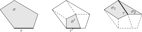
Figure 3.1. Examples of faces , , , and in
Lemma 3.3 (in the left and middle figure) and faces
, and in Lemma 3.4 (in the
right figure).
Lemma 3.4.
Let be an oriented polytope of dimension , and let be a polyhedral
subdivision of .
Assume that is a facet of two faces .
Then
(3.4)
Proof.
Being in the same situation as in the second case in Lemma 3.1,
it is easily verified that we may assume that ,
, and ,
where and .
Then the vector is a normal vector to pointing inwards to and is a normal vector to pointing inwards to . Letting be a basis of ,
by (3.1) and (3.2) the first term in the left-hand side of (3.4) equals
(3.5)
and the second term equals (3.5) with the opposite sign.
∎
4. Cellular resolutions of monomial ideals
Let us recall the construction of cellular resolutions due to
Bayer-Sturmfels [8].
Let be the polynomial ring .
We say that an (oriented) polyhedral cell complex is labeled if there
is a monomial
in associated with each vertex . An arbitrary face
of is then labeled by the least common multiple of the
labels of the vertices of , i.e., by
; should be
interpreted as .
We will sometimes be sloppy and not differ between the faces of a labeled complex and their labels.
Definition 4.1.
If and are two labeled polyhedral cell complexes, we say that refines
if refines as polyhedral cell complexes, i.e., , and each
face of is a union of faces in , and in addition, we require that
if , , and , then
.
Note that this implies that the ideal generated by the labels of the vertices of
must be contained in the ideal generated by the labels of the vertices of .
Let be a monomial ideal in , i.e., can be generated by
monomials. We will use the shorthand notation for the monomial
in .
It is easy to check that a monomial ideal has a
unique minimal set of generators that are monomials; assume that is a minimal set of monomial generators of .
Next, let be an oriented polyhedral cell complex with vertices
labeled by .
We will associate with a graded complex of free -modules: For
, let be the free -module with basis
and let the differential be defined by
(4.1)
Note that is a monomial when is a face of . The complex
is the cellular complexsupported on .
Note that, with the identification , the cokernel of equals .
The complex
is exact if the labeled complex satisfies a
certain acyclicity condition. More precisely, for ,
where , let denote the subcomplex of consisting
of all faces for which is divisible by
.
Then is
exact if and only if is acyclic, which means that
it is empty or has zero reduced homology, for all , see
[18, Proposition 4.5]. Note, in particular, that
the acyclicity does not depend on the orientation of .
When is exact we say that it is a cellular resolution of .
To put the cellular resolutions into the context of [5],
let us consider the vector bundle complex (2.2),
where for is a trivial bundle over
of rank equal to the number of faces in ,
with a global frame ,
endowed with the trivial metric, and where the
differential is given by (4.1).
We will say that the corresponding residue current is associated
with and denote it by , and we will use to denote
the coefficient of .
The induced sheaf complex (2.3) is exact if and only if is.
This follows from the standard fact that the ring of germs of
holomorphic functions at is flat over ,
see for example [25, Theorem 13.3.5].
We will think of monomial ideals sometimes as ideals in the polynomial
ring , sometimes as ideals in the ring of entire functions in
, and sometimes as ideals in the local ring .
4.1. The hull resolution
Given a monomial ideal in and ,
let
be the convex hull in of
.
Then is a unbounded
polyhedron in of dimension and the face poset (i.e., the set of faces
partially ordered by inclusion) of bounded faces of is independent of if
.
The hull complex of , introduced in [8], is the polyhedral cell
complex of all bounded faces of for . The vertices of
are precisely the points , where is a
minimal generator of , and thus admits a natural labeling.
The corresponding complex is a resolution of
; it is called the hull resolution.
Example 4.2.
Let be the complete intersection ideal .
Then, is the polyhedral cell complex consisting of the -simplex
in and its faces, where
.
The vertices of are labeled by
, respectively,
and we assume the faces are oriented so that the simplex with vertices
equals if .
Then the corresponding cellular complex is the Koszul complex
of , and
(4.2)
cf. Section 3.1 and Example 2.1. Note that a different orientation
of the top-dimensional simplex would permute the residue factors
in (4.2).
∎
The example shows that the hull complex of the complete intersection ideal
is the cellular complex consisting of an -simplex together with its
faces. In general, if is Artinian, is a polyhedral subdivision of such an
-simplex or, rather, it can be embedded as one, see, e.g., (the
proof of) Theorem 4.31 in [18].
We will need the following more precise description of this embedding.
To begin with, we note that an Artinian monomial ideal has monomials
of the form among its minimal monomial generators.
Note also that every other minimal generator has degree smaller than in .
Proposition 4.3.
Let be an Artinian monomial ideal with
among its minimal monomial generators. Let be the complete intersection ideal
. Then can be embedded as a refinement
of as labeled polyhedral cell complexes.
We will be sloppy and not always distinguish between the hull complex of and
its embedding.
Proof.
That refines as polyhedral cell complexes
is Theorem 4.31 in [18]. In fact, it follows from the proof
in [18] of that theorem that
it is a refinement also as labeled polyhedral cell complexes.
To see this, we begin by recalling (slightly differently described) the construction
of the embedding in that proof.
We know from Example 4.2 that consists of the faces
of the simplex with vertices
.
For a point , with , consider the line
through and . Since , intersects in a unique
point, which we denote . Moreover, since is contained in the set where ,
we get a map , which induces an embedding
of into by letting the faces of the embedded complex be the
images , where (with the same labeling).
Consider a face of such that
. Then the vertices of
must be contained in the set ,
since the are.
A vertex of with label has coordinates
, so if is contained in ,
then we must have in .
It follows that is of the form
,
and since each label of a minimal monomial generator is of degree at most
in , the same must hold for since it is the common multiple of such labels.
Hence, .
∎
Recall that a graded free resolution
is minimal if and only if for each , maps a basis
of to a minimal set of generators of , see,
e.g., [13, Corollary 1.5].
The hull resolution is not minimal in general, cf.
Example 6.1. However, if is a generic monomial
ideal in the sense of [9, 19],
the hull complex is simplicial, i.e., all faces are simplices, and it coincides with the
Scarf complex of , which is a minimal
resolution of , see [9].
The ideal is generic if whenever two distinct minimal
generators and
have the same positive degree in some variable, then there
exists a third generator that strictly divides the least common
multiple of and , meaning that divides
. Note that when all monomial ideals are generic. The Scarf complex of
is the collection of subsets
whose corresponding least common multiple
is unique.
We will prove a slightly more general version of Theorem 1.1.
If is a complete intersection ideal ,
by Example 4.2, is the polyhedral cell complex consisting of the faces
of an oriented -simplex , with vertices labeled by .
In particular, consists of only the simplex .
Theorem 5.1.
Let be an Artinian monomial ideal in .
Assume that is a cellular resolution of such that the underlying labeled polyhedral
cell complex refines the hull complex of a complete intersection ideal
, i.e., the -simplex with vertices labeled by
.
Then the associated residue current has one entry
for each -dimensional face of , and
where is the label of .
Theorem 1.1 corresponds to the case when equals ;
the refinement is given by Proposition 4.3, and the orientation
of is implicitly assumed to be such that for
each .
Proposition 5.2.
Let and be oriented labeled polyhedral cell complexes such that
refines , and let and
be the corresponding vector bundle complexes.
For let be the mapping
(5.1)
where the sum is over all that satisfy
.
Then the are holomorphic and the diagram (2.4) commutes.
We let and be as in Theorem 5.1, and .
Since , the complexes and
end at level .
Thus, identifying and and taking Proposition 5.2 for granted,
(2.5) yields
here we have used (4.2) for the last equality. Since
, the sum is over all , and
since the coefficient of
is
just
Since refines as a labeled polyhedral cell complex, each in (5.1) is holomorphic and thus the are holomorphic.
To show that (2.4) commutes, we first consider the case .
Pick .
Then
(5.2)
Here the first sum is over the facets of
, and the second sum is over the faces that are
contained in .
Moreover
(5.3)
Now the first sum is over the faces that are contained in
, whereas the second sum is over the facets of
.
Let be the -dimensional subcomplex
of faces of that are contained in and consider . Note that being a refinement of means that
is a polyhedral subdivision of .
Assume that is contained in a facet of
. Since , there is a unique such
, and thus the coefficient of (in the rightmost
expression) in (5.2)
equals
.
Moreover, is contained in the boundary of and
thus by Lemma 3.1 there is a unique such that . Therefore the coefficient of (in the rightmost
expression) in (5.3) is
.
By Lemma 3.3 these coefficients coincide.
If is not contained in any facet of , then
clearly the coefficient
of in (5.2)
is zero. Also, then is not contained in the boundary of ,
and thus
by Lemma 3.1, is a facet of exactly two faces . Hence the coefficient of in (5.3) is
which by Lemma 3.4 vanishes.
Since the sums in (5.2) and
(5.3) are only over that are in
, it follows that .
For , pick a vertex . Since is a polyhedral subdivision of
and is a vertex, the only with
is .
Thus . Note that maps
to . Thus .
We conclude that for
; in other words, the diagram (2.4) commutes.
∎
6. Comparison to previous results
In [27] the current constructed from a cellular resolution
of an Artinian monomial ideal was computed up to
multiplicative constants; Proposition 3.1 in [27] asserts that has one entry
for each face , which is of the form
(6.1)
for some , where
is the label of . The main novelty in this paper, except for the
new proof, is that we show that (or , depending on
the orientation of ) and thus give a complete
description of .
Let denote the annihilator ideal of ,
i.e., the ideal of germs of holomorphic functions at that satisfy .
Note that . A monomial ideal of this form is said to be
irreducible. Each monomial ideal can be
written as finite intersection of irreducible ideals; this is called an
irreducible decomposition of .
Since one has to annihilate each in order to annihilate
, Theorem 5.1 implies that, provided is a polyhedral
subdivision of ,
which gives an irreducible decomposition of . Here
is the multidegree of the label of .
If is a minimal resolution of this decomposition is irredundant in the sense that
no intersectand can be omitted. Each monomial ideal has a unique (monomial) irredundant irreducible decomposition.
Using that satisfies the duality
principle and results [9, Theorem 3.7] and
[18, Theorem 5.42] about irreducible decompositions, in [27], we could in some cases determine which
are
nonzero. If is a generic monomial ideal, Theorem 3.3 in that
paper says that is
nonzero if and only if is in the Scarf complex
(which is a subcomplex of any cellular resolution of ),
and if is a minimal resolution of each is
nonzero by Theorem 3.5 in [27].
Let us look at an example where
these theorems do not apply.
Example 6.1.
Consider the ideal
,
i.e., the square of the maximal ideal at in .
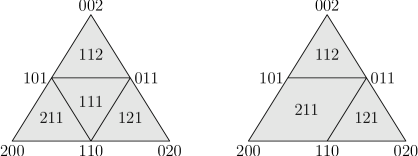
The hull complex of is a refinement
of the -simplex with the vertices labeled by , see Figure 6.1.
Figure 6.1. The hull complex of the ideal in Example 6.1
(labels on vertices and -faces) (left) and the cell complex of a minimal free
resolution of (right).
There are four faces in with
labels , ,
, and .
By Theorem 5.1, the current therefore has four entries: three entries of the
form
for , corresponding to the three corner triangles in , and one
component .
The hull resolution is not a minimal resolution of . In
particular,
is not generic.
By arguing as in the proofs of Theorems 3.3 and 3.5 in [27], using that
satisfies the duality principle and that
is the irredundant irreducible decomposition of ,
one can conclude that first three in (6.1) are non-zero,
but not that is.
A minimal resolution of is obtained by removing one of the edges
of the inner triangle in , see,
e.g., [18, Example 3.19]. The cell complex of one such resolution is depicted in
Figure 6.1.
Note that is a refinement of
(although different from )
so that Theorem 5.1 applies; the corresponding residue current consists of the three
entries , , and above.
∎
In [27] the current is computed as the push-forward of a
current on a toric log-resolution of . The computations are inspired
by [26], where Bochner-Martinelli residue currents, cf. Example 2.1, of monomial
ideals are computed, and they become quite involved. The coefficients
appear as certain integrals in the log-resolution and seem
to be hard to
compute in general.
The proof of Theorem 5.1 given here is more direct and much less technical than in [27].
It would be interesting to investigate whether the comparison formula
for residue currents could be used also to compute Bochner-Martinelli
residue currents. In [26] it was shown that if is an Artinian
monomial
ideal, the Bochner-Martinelli current of (a monomial sequence of
generators of) is a vector-valued
current with entries of the form (6.1), for certain exponents
. In some cases we can compute the
coefficients , e.g., if and each minimal generator
of the monomial ideal is a vertex of the so-called Newton polytope of ; the coefficients
are then equal to , see [28, Section 4.2].
If is the Koszul complex of and
is the Koszul complex of a complete
intersection ideal contained in , it is not hard to
explicitly find mappings so that the diagram (2.4)
commutes.
Indeed, let be a minimal set of generators of ,
ordered so that for ; note that
there are such generators since is Artinian. Identify the set of
generators with a section of a (trivial) rank
bundle . Similarly identify with a section of a rank
bundle and construct the Koszul complexes
and as in
Example 2.1. Now we can choose as the mapping
.
Theorem 3.2 in [15] then
gives a formula relating the currents and , the latter given
by (4.2). However, when is not a complete intersection and
thus does not end at level , the formula relating the currents is more involved than
(2.5); there appears an extra term, which seems hard to
compute in general, see [15, Equation (3.2)].
6.1. Non-Artinian monomial ideals
In [27] we also computed residue currents (up to nonvanishing factors) associated with cellular
resolutions of non-Artinian
monomial ideals.
The method in this paper is not as well adapted to resolutions of
non-Artinian ideals. First, to be able to use the simple form (2.5)
of the comparison formula for residue currents it is important that
is Cohen-Macaulay.
Second, even if is Cohen-Macaulay, there is in general no such
natural (resolution of an) ideal to compare with as the monomial complete
intersection ideal in the Artinian case.
Example 6.2.
Let be the ideal in .
Then
(6.2)
is a free resolution of .
Let be the corresponding vector bundle
complex.
Next, let be the regular sequence , and let be the Koszul
complex of . Then it is not hard to explicitly find the morphisms
, and . Since the ideals and are
Cohen-Macaulay we may apply the comparison formula
(2.5). A computation gives
Observe that is not symmetric in and , although the ideal
is. This is, however, not too surprising, since the resolution
(6.2) is not symmetric in and .
∎
A general strategy for computing the residue current associated with the
resolution of a
(monomial) Cohen-Macaulay ideal of codimension is to look for
a regular sequence contained in and then apply the comparison
formula (2.5) to and the Koszul complex of . One way of finding such a regular sequence is to consider sufficiently generic linear
combinations of the
generators of , as was done in Example 6.2.
However, when
the are not monomials the computation of the
current can become much more involved. Also,
although the complex is simple, it
may be hard to find the morphism in general.
If is a resolution of a non-Cohen-Macaulay
ideal, the comparison formula in [15] is more involved than
(2.5). For computations of residue currents in this case,
see [15, Section 5].
7. Relations to fundamental cycles
Our original motivation for computing the coefficients of
the entries (6.1) of
was that we wanted to understand the current
(7.1)
when is the residue current associated with a resolution
(2.3) of an
ideal sheaf of codimension and is the connection on induced by connections on .
Let be a complete intersection ideal, defined by a regular
sequence and let (2.2) be the Koszul complex of
, see Example 2.1, equipped with the trivial metrics
so that is the trivial connection .
Then (7.1) equals times the current
(7.2)
where is the current of integration along the fundamental
cycle of . The equality (7.2) was proved in [10].
Recall that for an Artinian ideal , the fundamental cycle
of is , where is the geometric multiplicity
of . For an arbitrary ideal , with irreducible components (i.e., irreducible
components of the radical ideal of ), the fundamental cycle of is
where are the geometric multiplicities of along .
The geometric multiplicity of along can be defined as the geometric
multiplicity of the Artinian ideal , where is the ideal of a generic
smooth variety transversal to . For more details regarding fundamental cycles,
see [14, Section 1.5].
Using the comparison formula for residue currents from [15],
we recently managed to prove that
(7.3)
for any resolution (2.3) of any equidimensional ideal (i.e., all
minimal primes are of the same dimension) ,
thus generalizing (7.2).
This factorization of the fundamental cycle is closely related to a
result by Lejeune-Jalabert, [17], who proved a cohomological
version of (7.3) for Cohen-Macaulay ideals, and it will be
the subject of the forthcoming paper [16].
For the residue current associated with the hull resolution of a
generic Artinian monomial ideal we can give an alternative proof of
(7.3) (with the trivial connection ) using Theorem 1.1. In fact, we get a
refinement of (7.3): For each permutation
of ,
(7.4)
where . For an
explanation of why the constant appears in the right hand side of
(7.4), but not in (7.3), see [16].
We will show how this works when . For , the computation
of gets more involved; the general case will therefore be
treated in the separate paper [29].
First, let us describe the geometric multiplicity of a monomial ideal .
Let denote the nonnegative real numbers and let
be the staircase
of . If
is Artinian, then is a bounded set in . The name
staircase is motivated by the shape of .
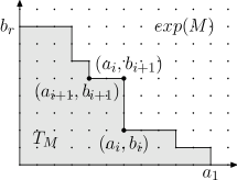
If each Artinian monomial ideal
is of the form for some integers
and . Then looks like a
staircase
with inner corners and outer corners ,
see Figure 7.1.
Figure 7.1. The staircase of an Artinian monomial ideal in . The lattice points above are the exponents of monomials in .
In general there is an “inner corner”
for each minimal generator of and one “outer
corner” for each intersectand in the
irredundant irreducible decomposition.
If is generic, there is a one-to-one correspondence between faces , with labels , and outer corners in .
The points in are precisely the exponents of monomials that are not in . In other words,
. It follows
that , where is the usual Euclidean
volume in .
Now assume that , and that is an Artinian ideal, minimally
generated by , and . Then is one-dimensional, with one vertex for
each generator and one edge , with label
, for each outer corner in .
The mappings in are given by
and
and
by Theorem 1.1,
Let us compute .
Note that
and
so that
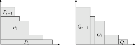
Let
for .
Then the form a partition of , cf. Figure
7.2 and, in particular, .
Note that . Hence (identifying with
)
Figure 7.2. Partitions of as rectangles and rectangles
.
By similar arguments we get that
, where for
, see Figure 7.2.
Again, the rectangles form a partition of and thus
(7.4) holds also for this permutation ( and
) of the variables. To conclude, we have proved
(7.3) for hull resolutions of monomial ideals in dimension
with .
For a generic Artinian monomial ideal
one can analogously define cuboids , where is
an outer corner of and is a permutation of , such that for a fixed , defines a partition of and moreover
Together with Theorem 1.1 this proves (7.4) and thus
(7.3) in this case.
However, for , the construction of the is
more delicate than that of and , see [29].
References
[1]M. Andersson: Residue currents and ideals of holomorphic functions, Bull. Sci. Math. 128 (2004) no. 6, 481–512.
[2]M. Andersson & H. Samuelsson: A Dolbeault-Grothendieck lemma on complex spaces via Koppelman
formulas, Invent. Math. 190 (2012), no. 2, 261–297.
[3]M. Andersson & H. Samuelsson: Weighted Koppelman formulas and the -equation on
an analytic space, J. Funct. Anal. 261 (2011), 777–802.
[4]M. Andersson & H. Samuelsson & J. Sznajdman: On the Briançon-Skoda theorem on a singular variety, Ann. Inst. Fourier 60 (2010), 417–432.
[5]M. Andersson & E. Wulcan: Residue currents with prescribed annihilator ideals, Ann. Sci. École Norm. Sup. 40 (2007) no. 6, 985–1007.
[6]M. Andersson & E. Wulcan: Decomposition of residue currents, J. Reine Angew. Math. 638 (2010), 103–118.
[7]M. Andersson & E. Wulcan: On the effective membership problem on singular varieties, Preprint, arXiv:1107.0388.
[8]D. Bayer & B. Sturmfels: Cellular resolutions of monomial modules, J. Reine Angew. Math. 502 (1998) 123–140.
[9]D. Bayer & I. Peeva & B. Sturmfels: Monomial resolutions, Math. Res. Lett. 5 (1998), no. 1-2, 31–46.
[10]N.r. Coleff & M.e. Herrera: Les courants résiduels associés à une forme méromorphe, Lect. Notes in Math. 633, Berlin-Heidelberg-New York (1978).
[11]A. Dickenstein & C. Sessa: Canonical representatives in moderate cohomology, Invent. Math. 80 (1985), 417–434.
[12]D. Eisenbud: Commutative algebra. With a view toward algebraic geometry, Graduate Texts in Mathematics, 160. Springer-Verlag, New York, 1995.
[13]D. Eisenbud: The geometry of syzygies. A second course in commutative algebra and algebraic geometry, Graduate Texts in Mathematics, 229. Springer-Verlag, New York, 2005.
[14]W. Fulton: Intersection theory. Ergebnisse der Mathematik und ihrer Grenzgebiete, Springer-Verlag, Berlin, 1984.
[15]R. Lärkäng: A comparison formula for residue currents, Preprint, arXiv:1207.1279.
[16]R. Lärkäng & E. Wulcan: Residue currents and fundamental cycles, In preparation.
[17]M. Lejeune-Jalabert: Remarque sur la classe fondamentale d’un cycle, C. R. Acad. Sci. Paris Sér. I Math. 292 (1981), no. 17, 801–804.
[18]E. Miller & B. Sturmfels: Combinatorial commutative algebra, Graduate Texts in Mathematics 227 Springer-Verlag, New York, 2005.
[19]E. Miller & B. Sturmfels & K. Yanagawa: Generic and cogeneric monomial ideals, Symbolic computation in algebra, analysis, and geometry (Berkeley, CA, 1998), J. Symbolic Comput. 29 (2000) no 4–5, 691–708.
[20]M. Passare: Residues, currents, and their relation to ideals of holomorphic functions, Math. Scand. 62 (1988), no. 1, 75–152.
[21]M. Passare: A calculus for meromorphic currents, J. Reine Angew. Math. 392 (1988), 37–56.
[22]M. Passare & A. Tsikh & A. Yger: Residue currents of the Bochner-Martinelli type, Publ. Mat. 44 (2000), 85–117.
[23]E. Spanier: Algebraic topology, McGraw-Hill Book Co., New York-Toronto, Ont.-London 1966.
[24]J. Sznajdman: A residue calculus approach to the uniform Artin-Rees lemma, Israel J. Math., to appear.
[25]J. L. Taylor: Several complex variables with connections to algebraic geometry and Lie groups, Graduate Studies in Mathematics, 46 American Mathematical Society, Providence, RI, 2002.
[26]E. Wulcan: Residue currents of monomial ideals, Indiana Univ. Math. J. 56 (2007), no. 1, 365–388.
[27]E. Wulcan: Residue currents constructed from resolutions of monomial ideals, Math. Z. 262 (2009), 235–253.