We study superconformal interfaces between ${\mathcal{N}}=(1,1)$ supersymmetric sigma models on tori, which preserve a $\widehat{u}(1)^{2d}$ current algebra. Their fusion is non-singular and, using parallel transport on CFT deformation space, it can be reduced to fusion of defect lines in a single torus model. We show that the latter is described by a semi-group extension of $O(d,d|\mathbb{Q})$, and that (on the level of Ramond charges) fusion of interfaces agrees with composition of associated geometric integral transformations. This generalizes the well-known fact that T-duality can be geometrically represented by Fourier-Mukai transformations.

Interestingly, we find that the topological interfaces between torus models form the same semi-group upon fusion. We argue that this semi-group of orbifold equivalences can be regarded as the $\alpha^{\prime}$ deformation of the continuous $O(d,d)$ symmetry of classical supergravity.

1 Introduction and summary of results

String theory compactified on a $d$-dimensional torus is invariant under the group $O(d,d|\mathbb{Z})$ of T-duality transformations [1]. This is the subgroup of U-dualities realized as automorphisms of the worldsheet sigma model. It is, however, also a subgroup of the much larger continuous group $O(d,d|\mathbb{R})$, which is the group of symmetries of the classical low-energy supergravity theory. This larger continuous symmetry is broken by quantum effects, in particular by the fact that the string momentum and winding vectors are quantized.

In this paper we show that a certain relic of $O(d,d|\mathbb{R})$ does survive as a symmetry of a subset of observables, at leading order in the string-loop expansion but to all orders in $\alpha{}^{\prime}$. These “quasi-symmetries” are implemented on the string worldsheet by topological interfaces (also referred to as defect lines). Topological interfaces have played a role in various contexts in recent years, see for example [2, 3, 4, 5, 6, 7, 8, 9, 10, 11, 12, 13, 14, 15, 16, 17, 18, 19, 20].

We are interested in topological interfaces between $d$-dimensional torus models which preserve a $\widehat{u}(1)^{2d}$ current algebra. It turns out that they are associated to elements $\hat{\Lambda}\in O(d,d|\mathbb{Q})$, the group of $O(d,d)$-matrices with rational entries. Their action on perturbative string states transforms an integer momentum and winding vector $\hat{\gamma}\in\mathbb{Z}^{d,d}$  to  $\hat{\Lambda}\hat{\gamma}$ whenever this is consistent with charge quantization, i.e. whenever $\hat{\Lambda}\hat{\gamma}$ is also in $\mathbb{Z}^{d,d}$; otherwise it projects the string state to zero. We will argue that the transformation also rescales the effective string-coupling constant by

$$\lambda_{\rm eff}\mapsto\lambda_{\rm eff}\,\sqrt{{\rm ind}(\hat{\Lambda})}\ .$$ (1)

Here, ${\rm ind}(\hat{\Lambda})$ denotes the index of the sublattice of charges that survives the projection, i.e. the smallest positive integer $K$ such that $K\hat{\Lambda}$ has only integer entries. Clearly these transformations can only be inverted if $K=1$, in which case they are the familiar T-dualities of string theory. The transformations for general $K$ do not form a group but rather a semi-group. It turns out to be a semi-group extension of $O(d,d|\mathbb{Q})$.

Topological interfaces for the free boson compactified on a circle, i.e. for $d=1$ have been analyzed in [8, 9]. We extend this analysis to torus models of arbitrary dimension $d\geq 1$, and also to theories with ${\cal N}=(1,1)$ worldsheet supersymmetry. Following [9] we actually compute the composition, or “fusion” of the more general superconformal but not necessarily topological interfaces. These do not separately commute with left and right moving superconformal algebras of the bulk SCFTs as is the case for topological ones, but only with the diagonal subalgebra. In the purely bosonic CFT this requires the introduction of a regulator and the subtraction of a divergent Casimir energy. For interfaces preserving a mutually compatible supersymmetry, on the other hand, the divergent Casimir energy cancels between bosons and fermions and there is no need for an infinite subtraction. The finite part of this energy contributes to the $g$ factor of the fusion product, just as expected from Cardy’s consistency condition [27].

Non-topological interfaces can be used to parallel transform the torus CFT along moduli space. This makes it possible to pull-back all interfaces to defects in a fixed, reference CFT, and to associate to them a universal defect algebra. The calculation of this algebra of non-topological defects is the main technical result in the present paper.

On a different note, conformal interfaces and defects can be realized as quantum junctions and quantum impurities in $(1+1)$-dimensional systems (for an introduction see [28, 29]). Our results on the fusion of such defects could thus find more direct applications in the study of the infrared properties of condensed-matter or statistical-mechanical systems. A by-product of our results is, for instance, the calculation of the fusion of conformal defects in the critical two-dimensional Ising model.

Conformal interfaces on the superstring worldsheet have been constructed recently in [30]. There, the Green-Schwarz formulation was used instead of the NSR formulation employed in this paper, and space-time instead of worldsheet supersymmetry was imposed. It was furthermore argued that the requirement of space-time supersymmetry forces the interface either to be topological or to be a (totally-reflecting) tensor product of supersymmetric D-branes. Since the $O(d,d|\mathbb{Q})$ quasi-symmetries are implemented on the NSR worldsheet by topological interfaces, it should be possible to rederive our results in the Green-Schwarz formulation adopted in [30] as well. However, we will not pursue this approach here.

The effective action for the moduli and the associated $u(1)^{2d}$ abelian gauge fields of toroidally-compactified string theory reads [31]

$$S=M^{2}_{\rm Planck}\int d^{10-d}x\sqrt{-g}\,\left[{1\over 8}{\rm Tr}(\partial_{\mu}M^{-1}\partial^{\mu}M)-{1\over 4}(F_{\mu\nu})^{T}(M^{-1})F^{\mu\nu}\right]\ ,$$ (2)

where

$$M=\left(\begin{matrix}G^{-1}&-G^{-1}B\\ BG^{-1}&G-BG^{-1}B\end{matrix}\right)$$ (3)

is a symmetric $O(d,d)$ matrix that obeys $M\hat{\eta}M=\hat{\eta}$, with $\hat{\eta}=(\begin{smallmatrix}0&{\bf 1}\\ {\bf 1}&0\end{smallmatrix})$. Here $G$ is the metric of the torus in the string frame, $B$ the NS 2-form field and $F_{\mu\nu}$ a $2d$-vector of gauge field strengths; $M_{\rm Planck}$ is the Planck scale of the effective (super)gravity. This action is invariant under the global $O(d,d)$ transformations $F_{\mu\nu}\mapsto\hat{\Lambda}F_{\mu\nu}$ and $M\mapsto\hat{\Lambda}M\hat{\Lambda}^{T}$ with $\hat{\Lambda}^{T}\hat{\eta}\hat{\Lambda}=\hat{\eta}$. Charge quantization restricts $\hat{\Lambda}$ to the T-duality subgroup $O(d,d|\mathbb{Z})$.

The topological interfaces constructed in this paper are associated to elements $\hat{\Lambda}$ of the larger group $O(d,d|\mathbb{Q})$, but they project out sublattices of charges whenever $\hat{\Lambda}\notin O(d,d|\mathbb{Z})$.

The matrix $M$ can be expressed in terms of an auxiliary “vielbein” field

$$M=2\,U^{T}U\ \leftrightarrow M^{-1}=2\,(U\hat{\eta})^{T}(U\hat{\eta})\ .$$ (4)

Using this vielbein one can define a vector of “physical” charges $\gamma=U\hat{\eta}\hat{\gamma}$, associated to a vector of integer charges $\hat{\gamma}$. The physical-charge vectors $\gamma$ take values in an even self-dual lattice $\Gamma^{d,d}$ of left and right momenta, with metric $\eta={\rm diag}({\bf 1},-{\bf 1})$. A general (super)conformal interface transforms $\gamma$ to $\Lambda\gamma$ with $\Lambda\in O(d,d)$. It is topological if $\Lambda\in O(d)\times O(d)$. Physical properties, such as the mass of a fundamental string, only depend on $\gamma$ modulo arbitrary $O(d)\times O(d)$ rotations.

One of the most interesting aspects of our analysis is the way in which the semi-group of topological interfaces acts on D-branes and on their Ramond charges. It turns out that just as the masses of fundamental string states, also the D-brane masses stay invariant. The vectors of integer Ramond charges, on the other hand, transform according to the spinor representation:

$$\hat{\gamma}_{D}\ \to\ \hat{S}\,\hat{\gamma}_{D}\ ,\qquad{\rm with}\ \ \ \hat{S}:=\sqrt{{\rm ind}(\hat{\Lambda})}\,S(\hat{\Lambda})\ \in\ GL(2^{d}|\mathbb{Z})\ .$$ (5)

Here $S$ is the spinor representation of $O(d,d|\mathbb{Q})$, while the square root of the index in the above expression can be interpreted as the rescaling (1) of the effective string coupling. Interestingly, the latter ensures that $\hat{S}$ acts as an endomorphism on the space of integer-component spinors. This should be contrasted to $\hat{\Lambda}$ whose action was restricted to a sublattice of the lattice of integer-component vectors.

The transformations (5) also have a nice geometric meaning. Namely, we show that the action of all superconformal $\widehat{u}(1)^{2d}$ preserving interfaces on the space of Ramond ground states descends from the action of geometric integral transformations on D-branes. If invertible, such transformations are known as Fourier-Mukai transformations, and it is indeed well known that T-dualities can be realized by Fourier-Mukai transformations [34, 35].

Although a topological interface with index $K\not=1$ cannot be inverted, its fusion with its parity-transform always yields a sum of invertible defects. The authors of [7] have argued very generally that interfaces with the above property separate CFTs that are related by orbifold constructions, and in particular preserve the sphere correlation functions of invariant untwisted states. Our results provide a concrete application of these ideas to the torus theories. The interfaces associated to elements of $O(d,d|\mathbb{Q})$ and $O(d,d|\mathbb{Z})$ are, in the language of [7], examples respectively of “duality defects” and the subclass of “group-like defects”.

Let us stress that $O(d,d|\mathbb{Q})$ is not an exact symmetry of string theory but an orbifold equivalence, i.e. a classical invariance of a subset of observables. It does, however, survive $\alpha^{\prime}$ corrections. It remains to be seen whether this “quasi-symmetry” has any profound meaning, or whether it is related to other fascinating glimpses on the arithmetic properties of string theory (see e.g. [36] and references therein).

The rest of the paper gives the technical details behind the claims made in this introduction. We begin in Section 2 with the construction of interfaces between bosonic circle theories that preserve $\widehat{u}(1)^{2}$ symmetry. We present both the explicit interface operators, and the corresponding boundary states of the two-boson theory that is obtained by folding the worldsheet along the interface. This material is already contained in [3, 9]. But we formulate it in a way that easily generalizes to higher target-space dimensions.

In Section 3 we extend the construction of Section 2 to superconformal interfaces between ${\cal N}=(1,1)$ supersymmetric $c=3/2$ circle theories. We emphasize the GSO projection, and in particular establish a precise correspondence of superconformal interfaces in the GSO projected theory and Cardy defects in the Ising model [2].

In Section 4 we derive the fusion of the $\widehat{u}(1)^{2}$-preserving superconformal interfaces between the $c=3/2$ circle theories. We show that fusion is non-singular for interfaces preserving the same supersymmetry, even if none of these interfaces is topological. We also explain how any interface can be parallel-transported to a defect in a given reference bulk theory, and compute the monoid of superconformal defects. This monoid turns out to be a semi-group extension of $O(1,1|\mathbb{Q})$, tensored for the GSO projected theory with the fusion algebra of the Ising model. We furthermore show that parallel transport provides a one-to-one correspondence of $\widehat{u}(1)^{2}$-preserving superconformal defects in circle theories and the $\widehat{u}(1)^{2}$-preserving topological interfaces starting in any given circle theory. This correspondence is compatible with fusion, so that the category of $\widehat{u}(1)^{2}$-preserving topological interfaces between circle theories can be completely described in terms of the monoid of $\widehat{u}(1)^{2}$-preserving superconformal defects. General conformal defects of the Ising model have been studied in [21, 23]. A by-product of our analysis is the fusion algebra of these Ising defects.

In Section 5 we explain the relation between the defect monoid and the $O(1,1|\mathbb{Q})$ quasi-symmetries of the supergravity action. In particular, we describe their action on perturbative string states on the one hand and D-brane charges on the other.

Section 6 contains the generalization to target space dimension $d>1$. We construct the $\widehat{u}(1)^{2d}$-preserving superconformal interfaces between $d$-dimensional torus models, and calculate their fusion. As in the case of $d=1$, also for arbitrary $d$, parallel transport reduces the fusion structure to the monoid of defects in a fixed reference torus model. We determine this monoid to be the extension (190) of $O(d,d|\mathbb{Q})$ by the semi-group of maximal rank sublattices of $\mathbb{Z}^{d,d}$ (where multiplication is given by intersection). In addition we also calculate the fusion of these defects with $\widehat{u}(1)^{2d}$-preserving superconformal boundary conditions. We tried to keep this section to some extent self contained, so as to make it readable independently of the detailed discussion of the $d=1$ case in Sections 2–4. It can therefore also serve as an overview of our analysis of interfaces.

In Section 7 we relate the action of the superconformal interfaces to geometric integral transformations. More precisely, we show that the interfaces act on Ramond ground states in the same way that corresonding geometric integral transformations act on D-brane charges. Even though we did not attempt to prove it, we believe that this is in fact true on the level of the full D-brane category, and that the interfaces fuse as the respective integral transformations compose.

Finally, in Section 8 we establish the one-to-one correspondence between conformal defect lines and topological interfaces in torus models. This extends the relation between the defect monoid on one hand, and $O(d,d|\mathbb{Q})$ quasi-symmetries of the effective supergravity action after compactification on a torus of arbitrary dimension $d\geq 1$.

In Appendix A we collect some conventions, and in Appendix B we prove an identity relating indices of certain sublattices which is needed for the calculation of the fusion of interfaces.

2 Free-boson interfaces preserving $\widehat{u}(1)^{2}$

We begin with a review of interfaces between two $c=1$ conformal field theories of free bosons compactified on a circles. We limit ourselves to interfaces preserving two $\widehat{u}(1)$ Kac-Moody symmetries. These interfaces were constructed and discussed in references [3, 9]. Here, we give a description that will easily generalize to higher target-space dimensions.

2.1 Interface operators versus boundary states

As explained in the above references, there are two different ways to think about interfaces: as operators mapping the states of CFT2 on the circle to those of CFT1; or as boundary conditions in the tensor-product theory CFT1$\otimes$CFT2^∗, where CFT2^∗ is the parity transform of CFT2. These two approaches are technically equivalent, but it will be useful in the sequel to keep them both at hand.

In this section CFT1 and CFT2 are theories of a free massless bosonic field $\phi$, compactified on circles of radii $R_{1}$ and $R_{2}$ respectively. Our conventions for $\phi$ are detailed in Appendix A.

In the first approach, conformal invariance is equivalent to the statement that the interface operator $I_{1,2}:{\mathcal{H}}_{2}\rightarrow{\mathcal{H}}_{1}$ between the Hilbert spaces of the two CFTs commutes with the Virasoro algebra $\{L_{n}-\tilde{L}_{-n},\,n\in\mathbb{Z}\}$. Since the Virasoro generators are quadratic in the $\widehat{u}(1)$ currents, the gluing conditions for the latter must be of the form

$$\left(\begin{array}[]{c}a^{1}_{n}\\ -\tilde{a}^{1}_{-n}\end{array}\right)I_{1,2}=I_{1,2}\,\Lambda\left(\begin{array}[]{c}a^{2}_{n}\\ -\tilde{a}^{2}_{-n}\end{array}\right)\qquad{\rm for}\qquad\Lambda\in O(1,1)\,.$$ (6)

Here $a^{1}$ and $a^{2}$ are the modes of the left-moving $\widehat{u}(1)$ currents of CFT1 and CFT2 respectively, while $\tilde{a}^{1}$ and $\tilde{a}^{2}$ are the modes of the right-moving currents. The matrix $\Lambda$ obeys $\Lambda^{T}\eta\Lambda=\eta$ with $\eta={\rm diag}(1,-1)$.

We stress that (6) does not describe all possible conformal gluing conditions of CFT1 with CFT2. First we have assumed that two affine $\widehat{u}(1)$ symmetries are preserved. Furthermore, taking an invertible gluing matrix $\Lambda$ discards the possibility that the interface factorize into separate boundary conditions for the currents of CFT1 and CFT2. In theories with $d>1$ bosons this assumption eliminates interfaces at which some of the currents of CFT2 (and also of CFT1) are fully reflected. Such non-generic interfaces can be analyzed separately, when needed.

To convert interfaces to boundary states one reflects CFT2 to CFT2^∗, so that both conformal theories are now defined on the half-cylinder $\tau\geq 0$. This exchanges the left- and right-moving modes

$$\left(\begin{array}[]{c}a^{2}_{n}\\ \tilde{a}^{2}_{n}\end{array}\right)\mapsto\left(\begin{array}[]{c}-\tilde{a}^{2}_{-n}\\ -a^{2}_{-n}\end{array}\right)\ .$$ (7)

The gluing conditions then become conformal boundary conditions for the tensor-product theory CFT1$\otimes$CFT2^∗. This is a two-boson theory whose target space is an orthogonal torus. The folding operation converts the interface into a boundary state that satisfies the gluing conditions

$$\left[\left(\begin{array}[]{c}a^{1}_{n}\\ -\tilde{a}^{1}_{-n}\end{array}\right)+\Lambda\left(\begin{array}[]{c}\tilde{a}_{-n}^{2}\\ -a_{n}^{2}\end{array}\right)\right]|I_{1,2}\rangle\!\rangle=0\,.$$ (8)

One can put these conditions in the equivalent but more standard form

$$\left[\left(\begin{array}[]{c}a_{n}^{1}\\ a_{n}^{2}\end{array}\right)+\mathcal{O}\left(\begin{array}[]{c}\tilde{a}_{-n}^{1}\\ \tilde{a}_{-n}^{2}\end{array}\right)\right]|I_{1,2}\rangle\!\rangle=0\,,$$ (9)

where $\mathcal{O}$ is the orthogonal matrix

$$\mathcal{O}(\Lambda)=\left(\begin{array}[]{cc}\Lambda_{12}\Lambda_{22}^{-1}&\Lambda_{11}-\Lambda_{12}\Lambda_{22}^{-1}\Lambda_{21}\\ \Lambda_{22}^{-1}&-\Lambda_{22}^{-1}\Lambda_{21}\end{array}\right)\,.$$ (10)

The inverse to relation (10) is

$$\Lambda(\mathcal{O})=\left(\begin{array}[]{cc}\mathcal{O}_{12}-\mathcal{O}_{11}\mathcal{O}_{21}^{-1}\mathcal{O}_{22}&\mathcal{O}_{11}\mathcal{O}_{21}^{-1}\\ -\mathcal{O}_{21}^{-1}\mathcal{O}_{22}&\mathcal{O}_{21}^{-1}\end{array}\right)\,.$$ (11)

Anticipating the generalization to higher target-space dimension $d$, we have written equations (10) and (11) so that they hold for current modes that are $d$-dimensional vectors. It is nevertheless instructive to make the mapping between $O(2)$ and $O(1,1)$ matrices more explicit. One notes that $O(2)$ has two disconnected components, while the number of disconnected components in $O(1,1)$ is four. These are related as follows:

$$\mathcal{O}=\left(\begin{array}[]{cc}{\rm cos}(2\vartheta)&{\rm sin}(2\vartheta)\\ -{\rm sin}(2\vartheta)&{\rm cos}(2\vartheta)\end{array}\right)\leftrightarrow\Lambda=\pm\left(\begin{array}[]{cc}{\rm cosh}\alpha&{\rm sinh}\alpha\\ {\rm sinh}\alpha&{\rm cosh}\alpha\end{array}\right)\left(\begin{array}[]{cc}1&0\\ 0&-1\end{array}\right)\ ,$$

$$\mathcal{O}=\left(\begin{array}[]{cc}{\rm cos}(2\vartheta)&{\rm sin}(2\vartheta)\\ {\rm sin}(2\vartheta)&-{\rm cos}(2\vartheta)\end{array}\right)\leftrightarrow\Lambda=\pm\left(\begin{array}[]{cc}{\rm cosh}\alpha&{\rm sinh}\alpha\\ {\rm sinh}\alpha&{\rm cosh}\alpha\end{array}\right)\ ,$$ (12)

where the rotation angle ${2\vartheta}\in(-\pi,\pi]$ is related to the rapidity $\alpha\in(-\infty,\infty)$ as follows:

$${\rm tanh}\alpha={\rm cos}(2\vartheta)\ ,$$ (13)

and the sign $\pm$ corresponds, respectively, to the ranges $\vartheta>0$ or $\vartheta<0$. Crossing the singular value $\vartheta=0$ amounts to jumping among the two disconnected components of $O(1,1)$ related by the reflection $-{\bf 1}$. Note that the identity gluing condition for an interface corresponds to a permutation gluing condition for the associated boundary condition, which glues the left (right) $\widehat{u}(1)$ current of CFT1 to the right (left) current of CFT2^∗.

Let us give a name to the sign that distinguishes the two components of the orthogonal group,

$${\rm det}\Lambda=-{\rm det}\mathcal{O}\ \mathrel{\stackrel{{\scriptstyle\mathrm{def}}}{{=}}}\ \varepsilon\ .$$ (14)

As shown in [9], when $\varepsilon=+1$ the interface corresponds to a D1-brane in the folded theory subtending an angle $\vartheta$ to the $\phi^{1}$ axis. For fixed compactification radii $R_{i}$ this angle cannot vary continuously, but is subject to the rationality condition

$${\rm tan}\vartheta={k_{2}R_{2}\over k_{1}R_{1}}\qquad{\rm if}\ \ \varepsilon=+1\ .$$ (15)

Here, $k_{1},k_{2}$ are arbitrary integers – the winding numbers of the associated D1-brane, which we take to be coprime in the following. For $\varepsilon=-1$ the folded interface corresponds to a D2/D0 bound state, and the rationality condition reads

$${\rm tan}\vartheta={2k_{2}R_{1}R_{2}\over k_{1}}\qquad{\rm if}\ \ \varepsilon=-1\ .$$ (16)

In this case, the integers $(k_{1},k_{2})$ are respectively the number of D2 -branes and the gauge flux threading through them. The latter is forced to be integer by Dirac’s quantization condition.

We also quote here the explicit form of the bosonic boundary states from reference [9]:

$$|\mathcal{O},\varphi\rangle\hskip-1.70717pt\rangle_{\rm bos}\ =\ \prod_{n=1}^{\infty}e^{\,{1\over n}\mathcal{O}_{ij}a_{-n}^{i}\widetilde{a}_{-n}^{j}}\ |\mathcal{O},\varphi\rangle_{\rm bos}\ ,$$ (17)

where the ground states for $\varepsilon=1$ and $\varepsilon=-1$ are respectively given by

$$|\mathcal{O},\varphi\rangle_{\rm bos}=\sqrt{k_{1}k_{2}\over{\rm sin}\,(2\vartheta)}\sum_{N,M=-\infty}^{\infty}e^{i{N}\varphi_{1}+iM\varphi_{2}}|k_{2}N,k_{1}N,k_{1}M,-k_{2}M\rangle\ ,\ {\rm and}\,$$

$$|\mathcal{O},\varphi\rangle_{\rm bos}=\sqrt{k_{1}k_{2}\over{\rm sin}\,(2\vartheta)}\sum_{N,M=-\infty}^{\infty}e^{i{N}\varphi_{1}+iM\varphi_{2}}|k_{1}M,-k_{1}N,k_{2}N,k_{2}M\rangle\,.$$ (18)

Here, $|N_{1},N_{2},M_{1},M_{2}\rangle$ denotes the highest-weight state with integer momenta $(N_{1},N_{2})$ and winding numbers $(M_{1},M_{2})$ in the two torus directions, while $\varphi$ parametrizes angle moduli of the boundary state (position and Wilson lines of the corresponding D-brane).

The $g$-factor is the coefficient of the $N=M=0$ ground state. Another important parameter is the reflection coefficient ${\cal R}$, defined quite generally in reference [23]. For the bosonic interfaces at hand, these two parameters are given by [9, 3]

$$g_{\rm bos}=\sqrt{{k_{1}k_{2}\over{\rm sin}(2\vartheta)}}\ ,\qquad{\cal R}={\rm cos}^{2}(2\vartheta)\ .$$ (19)

Note that while ${\cal R}$ varies continuously with the angle $\vartheta$, the $g$-factor depends non-trivially on its arithmetic properties. In string theory the $g$-factor is the (normalized) mass of the D-brane, viewed as a point particle in the non-compact spacetime. This (for $\varepsilon=+1$) depends on the length – not only on the orientation angle of the D1-brane. The quantization condition (15) ensures that this length, and hence the interface entropy, is finite.

Using the behavior (7) of the modes under folding, the boundary states are easily unfolded to interface operators. The mode contributions can be formally expressed as products of exponentials $I_{1,2}^{n,{\rm bos}}$. For $n>0$

$$I_{1,2}^{n,{\rm bos}}={\rm exp}\hskip-2.84526pt\left({1\over n}(a^{1}_{-n}\mathcal{O}_{11}\tilde{a}^{1}_{-n}-a^{1}_{-n}\mathcal{O}_{12}a^{2}_{n}-\tilde{a}^{1}_{-n}\mathcal{O}_{21}^{t}\tilde{a}^{2}_{n}+a^{2}_{n}\mathcal{O}_{22}^{t}\tilde{a}^{2}_{n})\right)\ ,$$ (20)

while the zero-mode contributions are given by

$$I_{1,2}^{0,{\rm bos}} = \sqrt{k_{1}k_{2}\over{\rm sin}(2\vartheta)}\hskip-2.27621pt\sum_{N,M=-\infty}^{\infty}e^{i{N}\varphi_{1}+iM\varphi_{2}}|k_{2}N,k_{1}M\,\rangle\langle k_{1}N,k_{2}M|\ ,\ {\rm and}$$

$$I_{1,2}^{0,{\rm bos}} = \sqrt{k_{1}k_{2}\over{\rm sin}(2\vartheta)}\sum_{N,M=-\infty}^{\infty}e^{i{N}\varphi_{1}+iM\varphi_{2}}|k_{1}M,k_{2}N\,\rangle\langle k_{1}N,k_{2}M|\$$ (21)

for $\varepsilon=\det\Lambda=+1$ and $-1$, respectively. Using a slightly abusive notation we may express the complete interface operator as

$$I_{1,2}^{\rm bos}=\prod_{n\geq 0}I_{1,2}^{n,{\rm bos}}\,,$$ (22)

with the implicit understanding that the positive-frequency modes of CFT1 act on the left and those of CFT2 on the right of the map $I_{1,2}^{0,{\rm bos}}$. This latter map implements the zero-mode gluing conditions on the ground states of the two $\widehat{u}(1)$ Kac-Moody algebras.

2.2 Quantization and sublattices

The quantization conditions (15) and (16) cannot be generalized as such to higher target-space dimensions. To put them in a more convenient form, note that in addition to the $O(1,1)$ matrix $\Lambda$ which enters in the gluing of the $\widehat{u}(1)$ currents, the interface is characterized by the choice of the bulk radii, $R_{1}$ of CFT1 and $R_{2}$ of CFT2. More explicitly, the corresponding charge lattices can be written as (here $j=1,2$)

$$\Gamma_{j}=\left\{\left(\begin{matrix}\mbox{$N/2R_{j}$}+\mbox{$MR_{j}$}\\ \mbox{$-N/2R_{j}$}+\mbox{$MR_{j}$}\end{matrix}\right)\Bigl{|}N,M\in\mathbb{Z}\right\}\ =\ U_{j}\,\mathbb{Z}^{1,1}\ ,$$ (23)

where the matrices

$$U_{j}=\left(\begin{matrix}\mbox{$1/2R_{j}$}&\mbox{$R_{j}$}\\ \mbox{$-1/2R_{j}$}&\mbox{$R_{j}$}\end{matrix}\right)$$ (24)

are the “vielbeins” introduced in (4) and $\mathbb{Z}^{1,1}$ is the lattice of integer momenta and windings. The transformation (23) corresponds precisely to the change of basis from the physical left and right $u(1)$ charges to integer momentum and winding, which has been mentioned in the introduction.

Note that states of CFT2 with physical charge vector $\gamma\in\Gamma_{2}$ are mapped to states of CFT1 with physical charge vector $\Lambda\gamma$. If $\Lambda\gamma\in\Gamma_{1}$ then $|\Lambda\gamma\rangle\langle\gamma|$ does indeed contribute to the zero-mode operator $I_{1,2}^{0,{\rm bos}}$. Otherwise, all CFT2 states in the $\widehat{u}(1)^{2}$ module with highest-weight vector $|\gamma\rangle$ are mapped to zero by $I_{1,2}$. The CFT2 charge vectors that contribute to the zero-mode sum lie therefore in the intersection sublattice of physical charges

$$\Gamma_{1,2}^{\Lambda}\ :=\ \{\gamma\in\Gamma_{2}|\Lambda\gamma\in\Gamma_{1}\}\,=\,\Gamma_{2}\cap\Lambda^{-1}\Gamma_{1}\,=\,\Gamma_{2}\cap\Lambda^{-1}U_{1}U_{2}^{-1}\Gamma_{2}\,.$$ (25)

This is mapped by $\Lambda$ to the sublattice of CFT1 charge vectors

$$\Gamma_{2,1}^{\Lambda^{-1}}\ :=\ \{\gamma\in\Gamma_{1}|\Lambda^{-1}\gamma\in\Gamma_{2}\}\,=\,\Gamma_{1}\cap\Lambda\Gamma_{2}\,=\,\Gamma_{1}\cap\Lambda U_{2}U_{1}^{-1}\Gamma_{1}\,,$$ (26)

where $\Gamma_{1}=U_{1}U_{2}^{-1}\Gamma_{2}$. The quantization conditions (15), (16) ensure that $\Gamma_{1,2}^{\Lambda}$ is a maximal-rank sublattice of $\Gamma_{2}$ (or equivalently that $\Gamma_{2,1}^{\Lambda^{-1}}$ is a maximal-rank sublattice of $\Gamma_{1}$). Gluing matrices obeying this maximal-rank condition will be referred to as “admissible” gluing matrices.

This condition is more transparent in the canonical basis of integer winding and momentum. The gluing of these integer-charge vectors is implemented by $\hat{\Lambda}:=U_{1}^{-1}\Lambda U_{2}$. This is a $O(1,1)$ matrix that leaves invariant the (off-diagonal) metric $\hat{\eta}=\left(\begin{smallmatrix}0&1\\ 1&0\end{smallmatrix}\right)$ on $\mathbb{Z}^{1,1}$. It can be read off easily from the zero-mode maps (21) with the result:

$$\hat{\Lambda}=\left(\begin{matrix}k_{2}/k_{1}&0\\ 0&k_{1}/k_{2}\end{matrix}\right)\ \ \quad{\rm or}\quad\ \ \hat{\Lambda}=\left(\begin{matrix}0&1\\ 1&0\end{matrix}\right)\left(\begin{matrix}k_{2}/k_{1}&0\\ 0&k_{1}/k_{2}\end{matrix}\right)\$$ (27)

for $\varepsilon=+1$ or $\varepsilon=-1$, respectively. In this canonical basis the admissible gluing conditions are, therefore, in one-to-one correspondence with elements of $O(1,1|\mathbb{Q})$, the group of $O(1,1)$ matrices with rational entries. This form of the quantization condition will generalize easily to higher target-space dimension.

For general $k_{1},k_{2}$, the transformations (27) do not map all integer vectors to integer vectors. Only the sublattice

$$U_{2}^{-1}\Gamma_{1,2}^{\Lambda}=\mathbb{Z}^{1,1}\cap\hat{\Lambda}^{-1}\mathbb{Z}^{1,1}=k_{1}\mathbb{Z}\oplus k_{2}\mathbb{Z}\$$ (28)

is mapped back to $\mathbb{Z}^{1,1}$, more precisely to the sublattice

$$U_{1}^{-1}\Gamma_{2,1}^{\Lambda^{-1}}=\mathbb{Z}^{1,1}\cap\hat{\Lambda}\mathbb{Z}^{1,1}=k_{2}\mathbb{Z}\oplus k_{1}\mathbb{Z}\ \ {\rm or}\ \ k_{1}\mathbb{Z}\oplus k_{2}\mathbb{Z}$$ (29)

for $\varepsilon=+1$ and $\varepsilon=-1$, respectively. The index

$${\rm ind}(\hat{\Lambda}):={\rm ind}(\mathbb{Z}^{1,1}\cap\hat{\Lambda}^{-1}\mathbb{Z}^{1,1}\subset\mathbb{Z}^{1,1})=|k_{1}k_{2}|$$ (30)

of this intertwiner sublattice in the charge lattice $\mathbb{Z}^{1,1}$ will play a key role in what follows. It is convenient to define the projector

$$\Pi_{\hat{\Lambda}}|\hat{\gamma}\rangle:=\begin{cases}|\hat{\gamma}\rangle&\ \ {\rm if}\ \ \ {\hat{\Lambda}}\hat{\gamma}\in\mathbb{Z}^{1,1}\,,\\ 0&\ \ {\rm otherwise}\end{cases}$$ (31)

on sectors with charges in this sublattice. Using these definitions and the identities $|\Lambda_{22}|={\rm cosh}\alpha={|\sin(2\vartheta)|}^{-1}$, see (12) and (13), we can put the ground state maps (21) in the more elegant form

$$I_{1,2}^{0,{\rm bos}}\ =\ \sqrt{{\rm ind}({\hat{\Lambda}})\,|\Lambda_{22}|}\ \sum_{\hat{\gamma}\in\mathbb{Z}^{1,1}}e^{2\pi i\varphi(\hat{\gamma})}|\hat{\Lambda}\hat{\gamma}\rangle\langle\hat{\gamma}|\,\Pi_{\hat{\Lambda}}\ ,$$ (32)

where $\varphi$ is some linear form on $\mathbb{Z}^{1,1}$. This expression easily generalizes to higher dimensions.

We conclude this section with the following remark: the interfaces discussed here can be uniquely specified by the data $(\hat{\Lambda},\varphi,U_{1},U_{2})$, where $\hat{\Lambda}\in O(1,1|\mathbb{Q})$ while $U_{j}\in O(1,1|\mathbb{R})$ determine the bulk radii. Interestingly, in the expression (32) for the zero-mode sum only $\Lambda_{22}$ depends on these bulk radii. Furthermore, as explained in reference [9], to any choice of the discrete data $\hat{\Lambda}$ and of $R_{2}$ there corresponds an $R_{1}$,

$$R_{1}=f_{\hat{\Lambda}}(R_{2}):=\begin{cases}\ \left|{k_{2}\over k_{1}}\right|R_{2}&\ \ {\rm if}\ \varepsilon=+1\\ \left|{k_{1}\over k_{2}}\right|{1\over 2R_{2}}&\ \ {\rm if}\ \varepsilon=-1\ ,\end{cases}$$ (33)

such that $|\Lambda_{22}|\hskip-0.85358pt=\hskip-0.85358pt|{\rm sin}(2\vartheta)|\hskip-0.85358pt=\hskip-0.85358pt1$ and the $g$-factor is minimized. Indeed from (24), (27) and (33) one can compute $\Lambda=U_{1}\hat{\Lambda}U_{2}^{-1}={\rm diag}(\pm 1,\pm 1)$, so that the gluing matrix for the $u(1)^{2}$ currents is a $O(1)\times O(1)$ matrix. This means that these interfaces commute with both, the left and right Virasoro algebra, and are therefore topological. For a given $\hat{\Lambda}$, they exist for any $R_{2}$, and the corresponding interface operators do not exhibit an explicit $R_{2}$ dependence.

A more detailed discussion of this point in the context of torus models of arbitrary target space dimension $d$ can be found in Section 8.

3 ${\cal N}=1$ supersymmetry

We will now extend the discussion of the previous section to the ${\cal N}=(1,1)$ supersymmetric CFT, consisting of a free boson $\phi$ and a free Majorana fermion with left and right components $\psi$ and $\tilde{\psi}$. Interfaces preserving ${\cal N}=1$ supersymmetry have been constructed in reference [3]. Here we complete this construction in the GSO projected theory, where the interface operators can have a non-trivial Ramond sector.

3.1 Superconformal $\widehat{u}(1)$ invariant boundary states

As a warm up we will first consider the superconformal boundary states of the $c=3/2$ theory. We limit ourselves to states preserving a $\widehat{u}(1)$ symmetry – for a more general discussion see references [37, 38]. Besides the Virasoro generators $\{L_{n}-\tilde{L}_{-n},\,n\in\mathbb{Z}\}$, these states are annihilated by the combinations $\{G_{r}-i\eta_{\rm S}\tilde{G}_{-r},\,\forall r\}$ of modes of the left and right supersymmetry currents. The choice of gluing condition $\eta_{\rm S}=\pm 1$ specifies which of the two possible supersymmetries is preserved. Notice the factor of $i$ in these combinations; it ensures that the supersymmetry generators anticommute into the Virasoro generators that annihilate the boundary state.

States preserving a $\widehat{u}(1)$ symmetry are annihilated by the combinations $\{a_{n}-\varepsilon\widetilde{a}_{-n},\,n\in\mathbb{Z}\}$ of modes of the left and right $\widehat{u}(1)$ currents. The choice of the sign $\varepsilon=1$ or $\varepsilon=-1$ distinguishes between Dirichlet and Neumann boundary conditions. In combination with superconformal invariance these gluing conditions force separate gluing conditions on the fermionic fields. Namely, the fermionic modes $\{\psi_{r}-i\epsilon\,\tilde{\psi}_{-r},\,\forall r\}$ with $\epsilon\equiv\varepsilon\eta_{\rm S}$ also have to annihilate the boundary state. Having to satisfy gluing conditions for bosons and fermions independently, the boundary states factorize into tensor products of bosonic and fermionic boundary states,

$$|{\cal B}\rangle\!\rangle_{\rm full}=|{\cal B}\rangle\!\rangle_{\rm bos}\otimes|{\cal B}\rangle\!\rangle_{\rm ferm}\ .$$ (34)

The Dirichlet and Neumann boundary states for the boson are well-known (see for example [39, 40] and references therein) but we repeat them here for the reader’s convenience:

$${\rm D:}\quad|+,\varphi\rangle\!\rangle_{\rm bos}\ =\ \prod_{n=1}^{\infty}{\rm exp}\left({1\over n}a_{-n}\tilde{a}_{-n}\right)\ \Bigl{(}{1\over\sqrt{2R}}\sum_{N=-\infty}^{\infty}e^{-i{N}\varphi}|N,0\rangle\Bigr{)}\ ,$$

$${\rm N:}\quad|-,\varphi\rangle\!\rangle_{\rm bos}\ =\ \prod_{n=1}^{\infty}{\rm exp}\left(-{1\over n}a_{-n}\tilde{a}_{-n}\right)\ \Bigl{(}\sqrt{R}\sum_{M=-\infty}^{\infty}e^{-iM\varphi}|0,M\rangle\Bigr{)}\ ,$$ (35)

where $|N,M\rangle$ is the normalized ground state in a given momentum and winding sector, and the angle $\varphi$ corresponds, in string-theoretic language, to the position of a D-particle on the circle or the Wilson line of a winding D-string. The $g$-factors of the above boundary states, $\sqrt{R}$ or $\sqrt{1/2R}$, will be important for our discussion later on.

The fermionic boundary states are linear combinations of

$$|{\rm NS},\epsilon\rangle\hskip-1.99168pt\rangle\ =\prod_{r\in{\mathbb{N}}-{1\over 2}}e^{i\epsilon\psi_{-r}\tilde{\psi}_{-r}}|0\rangle_{\rm NS}\ ,\qquad|{\rm R},\epsilon\rangle\hskip-1.99168pt\rangle\ =2^{1\over 4}\prod_{r\in{\mathbb{N}}}e^{i\epsilon\psi_{-r}\tilde{\psi}_{-r}}|\epsilon\rangle_{\rm R}\ ,$$ (36)

where $\mathbb{N}$ denotes the set of positive integers. Our conventions for the fermion field are given in Appendix A. The normalized Ramond ground states $|\epsilon\rangle_{\rm R}$ form a representation of the algebra of fermionic zero modes,

$$\psi_{0}|\pm\rangle_{\rm R}={1\over\sqrt{2}}e^{\pm i\pi/4}|\mp\rangle_{\rm R}\ ,\qquad\tilde{\psi}_{0}|\pm\rangle_{\rm R}={1\over\sqrt{2}}e^{\mp i\pi/4}|\mp\rangle_{\rm R}\ .$$ (37)

The cylinder partition functions associated with the above boundary states can be computed using standard techniques. Setting $H=L_{0}+\widetilde{L}_{0}$ for the Hamiltonian and $q=e^{-\tau}$ (with $\tau$ real) one finds:

$$\langle\hskip-1.70717pt\langle{\rm NS},\epsilon|\,q^{H}\,|{\rm NS},\epsilon\,\rangle\hskip-1.70717pt\rangle\,=\,q^{-{1\over 24}}\prod_{r\in\mathbb{N}-1/2}(1+q^{2r})\,=\,\left|{\theta_{3}\over\eta}\right|^{1/2}\ ,$$

$$\langle\hskip-1.70717pt\langle{\rm NS},\epsilon|\,q^{H}\,|{\rm NS},-\epsilon\,\rangle\hskip-1.70717pt\rangle\,=\,q^{-{1\over 24}}\prod_{r\in\mathbb{N}-1/2}(1-q^{2r})\,=\,\left|{\theta_{4}\over\eta}\right|^{1/2}\ ,$$

$$\langle\hskip-1.70717pt\langle{\rm R},\epsilon|\,q^{H}\,|{\rm R},\epsilon\,\rangle\hskip-1.70717pt\rangle\,=\,\sqrt{2}\,q^{{1\over 12}}\prod_{r\in\mathbb{N}}(1+\,q^{2r})\,=\,\left|{\theta_{2}\over\eta}\right|^{1/2}\ .$$ (38)

Here $\eta$ and $\theta_{a}$ denote the familiar Dedekind-eta and Jacobi-theta functions. The partition function between Ramond contributions of opposite $\epsilon$ vanishes.

The boundary states of the unprojected fermion theory are the states $|{\rm NS},\pm\,\rangle\hskip-1.70717pt\rangle$. We are interested in the boundary states of the GSO projected theory, which can be thought of as an orbifold by the $\mathbb{Z}_{2}$ group generated by the operator $(-1)^{F+\widetilde{F}}$. Here $F$ and $\widetilde{F}$ denote left and right fermion numbers respectively. Since $|{\rm NS},\pm\,\rangle\hskip-1.70717pt\rangle$ are invariant under the orbifold group, they must be resolved by additional contributions from the twisted sectors – the Ramond sector in the case at hand. This gives

$$|\epsilon\rangle\hskip-1.70717pt\rangle_{\rm ferm}={1\over\sqrt{2}}\left(|{\rm NS},\epsilon\rangle\hskip-1.70717pt\rangle\pm|{\rm R},\epsilon\rangle\hskip-1.70717pt\rangle\right)\ ,$$ (39)

with the normalization ${|\mathbb{Z}_{2}|}^{-1/2}={1/\sqrt{2}}$  chosen as usual so that the identity appears in the direct (open-string) channel with multiplicity one. To obtain the boundary states in the orbifold theory, one only needs to project on the invariant subsectors, which is done by taking appropriately normalized orbits under the action of the orbifold group.

Since $(-1)^{F+\widetilde{F}}$ anti-commutes with all the fermionic modes $\psi_{r}$ and $\widetilde{\psi}_{r}$, its action is completely determined by its action on the ground states $|0\rangle_{\rm NS}$ and $|\epsilon\rangle_{R}$. On the NS ground state it acts trivially, but there are two consistent choices on the twisted, i.e. the Ramond ground states:

$$(-1)^{F+\widetilde{F}}=\left\{\begin{array}[]{cc}-2i\psi_{0}\widetilde{\psi}_{0}&{\rm 0A}\\ 2i\psi_{0}\widetilde{\psi}_{0}&{\rm 0B}\end{array}\,.\right.$$ (40)

By reference to string theory, we call the two choices “type 0A” and “type 0B”. They are related by the $\mathbb{Z}_{2}$ duality that exchanges the spin with the disorder operator of the Ising model, which is the orbifold CFT.

The construction of the projected boundary states in orbifold theories has been discussed in [41]. One simply sums the images under the action of the orbifold group $G$, and normalizes the result by $(|{\rm Stab}_{G}|/|G|)^{{1\over 2}}$, where the stabilizer ${\rm Stab}_{G}$ is the subgroup of $G$ which leaves the original unprojected boundary state invariant . It can be seen that in addition to $|{\rm NS},\epsilon\rangle\!\rangle$ also $|{\rm R},-\rangle\!\rangle$ is invariant under the $\mathbb{Z}_{2}$ action in the 0A orbifold, while $|{\rm R},+\rangle\!\rangle$ is invariant in the 0B orbifold. On the other hand $(-1)^{F+\widetilde{F}}$ multiplies $|{\rm R},+\rangle\!\rangle$ (respectively $|{\rm R},-\rangle\!\rangle$) by $-1$. Thus, applying the orbifold construction to the boundary states (39) yields the boundary states

$$|{\rm{charged}},\pm\rangle\hskip-1.99168pt\rangle_{\rm ferm}^{\rm 0A} = {1\over\sqrt{2}}\left(|{\rm NS},-\rangle\hskip-1.99168pt\rangle\ \pm|{\rm R},-\rangle\hskip-1.99168pt\rangle\right),$$ (41)

$$|{\rm{neutral}}\rangle\hskip-1.99168pt\rangle_{\rm ferm}^{\rm 0A} = |{\rm NS},+\rangle\hskip-1.99168pt\rangle\$$

for the 0A orbifold, and

$$|{\rm{charged}},\pm\rangle\hskip-1.99168pt\rangle_{\rm ferm}^{\rm 0B} = {1\over\sqrt{2}}\left(|{\rm NS},+\rangle\hskip-1.99168pt\rangle\ \pm|{\rm R},+\rangle\hskip-1.99168pt\rangle\right),$$ (42)

$$|{\rm{neutral}}\rangle\hskip-1.99168pt\rangle_{\rm ferm}^{\rm 0B} = |{\rm NS},-\rangle\hskip-1.99168pt\rangle\$$

for the 0B orbifold. By reference to string theory, we call a boundary condition charged if it has a non-vanishing R-charge, i.e. if it couples to the Ramond ground states.

Another way of stating this result is that the fermion-parity projection eliminates $|+\rangle_{\rm R}$ in the type-0A theory, and $|-\rangle_{\rm R}$ in the type-0B theory. The projection also removes the Ishibashi states built on these Ramond ground states, leaving three independent boundary states in each theory. Cardy’s condition [27] fixes the precise linear combinations.

Indeed, the GSO-orbifold of the free fermionic theory is nothing but the Ising model, a well-known rational CFT with three primary fields of conformal weights $h=\tilde{h}=0,{1/2},{1/16}$. Boundary states in this theory can be obtained by means of Cardy’s construction, which expresses them in terms of the associated Ishibashi states as [27]

$${{{\rm spin\,up}}}:\qquad\ \ \ \ |0\rangle\hskip-1.99168pt\rangle_{\rm C}\ ={1\over\sqrt{2}}\,|0\rangle\hskip-1.99168pt\rangle_{\rm Ish}+{1\over\sqrt{2}}\,|{1\over 2}\rangle\hskip-1.99168pt\rangle_{\rm Ish}+{1\over 2^{1/4}}|{1\over 16}\rangle\hskip-1.99168pt\rangle_{\rm Ish}\ ,$$

$${\rm spin\,down}:\qquad|{1\over 2}\rangle\hskip-1.99168pt\rangle_{\rm C}\ ={1\over\sqrt{2}}\,|0\rangle\hskip-1.99168pt\rangle_{\rm Ish}+{1\over\sqrt{2}}\,|{1\over 2}\rangle\hskip-1.99168pt\rangle_{\rm Ish}-{1\over 2^{1/4}}|{1\over 16}\rangle\hskip-1.99168pt\rangle_{\rm Ish}\ ,$$

$${{{\rm spin\,free}}}:\qquad\ \ |{1\over 16}\rangle\hskip-1.99168pt\rangle_{\rm C}\ =|0\rangle\hskip-1.99168pt\rangle_{\rm Ish}-|{1\over 2}\rangle\hskip-1.99168pt\rangle_{\rm Ish}\ .$$ (43)

The boundary conditions of the Ising spin are indicated on the left.

One can easily identify the states in (36) with the Ising Ishibashi states by comparing the cylinder partition functions. The result is

$$|{\rm NS},\pm\rangle\hskip-1.99168pt\rangle=|0\rangle\hskip-1.99168pt\rangle_{\rm Ish}\mp|{1\over 2}\rangle\hskip-1.99168pt\rangle_{\rm Ish}\qquad{\rm and}\qquad|{\rm R},-\rangle\hskip-1.99168pt\rangle\ ={2^{-{1\over 4}}}\,|{1\over 16}\rangle\hskip-1.99168pt\rangle_{\rm Ish}\ .$$ (44)

Thus, the boundary states constructed above are related with the Ising boundary states by

$$|{\rm charged},+\rangle\!\rangle_{\rm ferm}^{\rm 0A}=|0\rangle\!\rangle_{\rm C}\,,\quad{\rm spin\,up}\,,$$

$$|{\rm charged},-\rangle\!\rangle_{\rm ferm}^{\rm 0A}=|{1\over 2}\rangle\!\rangle_{\rm C}\,,\quad{\rm spin\,down}\,,$$

$$|{\rm neutral}\rangle\!\rangle_{\rm ferm}^{\rm 0A}=|{1\over 16}\rangle\!\rangle_{\rm C}\,,\quad{\rm spin\,free}\,.$$ (45)

The charged states correspond to the fixed-spin boundary conditions of the Ising model; they have non-vanishing one-point functions with the Ramond ground state. The neutral boundary state, on the other hand, corresponds to the free-spin boundary condition of the Ising model; its one-point function with the Ramond vacuum vanishes.

Let us now go back to the $c={3\over 2}$ theory and put together the bosonic and fermionic states. In the unprojected theory this gives

$$|\varepsilon,\varphi,\eta_{\rm S}\rangle\!\rangle_{\rm full}=|\varepsilon,\varphi\rangle\!\rangle_{\rm bos}\otimes|{\rm NS},\varepsilon\eta_{\rm S}\rangle\!\rangle$$ (46)

where $|\varepsilon,\varphi\rangle\!\rangle_{\rm bos}$ is one of the states (35). After GSO projection, on the other hand, on finds for instance in the type 0A model

$$|\varepsilon,\varphi,\eta_{\rm S}\rangle\!\rangle_{\rm full} = |\varepsilon,\varphi\rangle\!\rangle_{\rm bos}\otimes\sqrt{{|{\rm Stab}_{G}|\over|G|}}\sum_{\rm\mathbb{Z}_{2}\ orbit}|\varepsilon\eta_{\rm S}\rangle\!\rangle_{\rm ferm}$$ (47)

$$= |\varepsilon,\varphi\rangle\!\rangle_{\rm bos}\otimes|h\rangle\!\rangle_{\rm C}\ ,$$ (48)

where $|\varepsilon\eta_{\rm S}\rangle\!\rangle_{\rm ferm}$ was defined in (39) and the orbit sum gives one of the three Cardy states of the Ising model, as just explained.

The supersymmetry preserved by boundary states in the GSO projected theories is summarized in table 1. As shown there, a charged Neumann and a neutral Dirichlet state preserve the $\eta_{S}=+1$ supersymmetry in the type 0A model. The second supersymmetry, $\eta_{S}=-1$, is preserved by a neutral Dirichlet and a charged Neumann state.

	Dirichlet	Neumann
charged	-	+
neutral	+	-

Table 1: The value of $\eta_{\rm S}$ determining which superconformal symmetry is preserved by boundary states of the $c={3\over 2}$ type-0A model. The boundary states are tensor products of a Dirchlet or Neumann boundary state for the boson with a fermion state in (41) or (3.1). Charged states are doubly-degenerate. In the type-0B theory the sign of $\eta_{\rm S}$ has to be reversed.

Let us recapitulate all the signs that entered the construction of boundary states. The gluing condition of the $\widehat{u}(1)$ current is determined by $\varepsilon$, and the unbroken supersymmetry by $\eta_{\rm S}$. Together these fix the gluing condition $\epsilon=\varepsilon\eta_{\rm S}$ of the fermionic field. If the Ishibashi state implementing this gluing condition in the Ramond sector survives the GSO projection, the boundary state is charged – i.e. it has non-vanishing overlap with the Ramond ground state. If it does not the (superconformal) boundary state is neutral.

We close this subsection with two remarks. First by analogy with the $g$-factor, which is the projection of a boundary state on the NS ground state, one can define the Ramond charge(s) as the projection onto Ramond ground state(s). In the case at hand, these two quantities are related in a way reminiscent of a BPS condition for supersymmetric D-branes. There is however no space-time supersymmetry in the present context; the relation is accidental as will become clear later.

The second remark concerns the cylinder partition function. As is well known, for any two boundary states preserving the same superymmetry, i.e. with the same $\eta_{\rm S}$, this partition function is finite in the limit $\tau\to 0$. The singular behavior in the bosonic sectors is exactly cancelled by the contribution of the fermions, as follows from the absence of tachyons in the open-string channel. The generalization of this fact to superconformal interfaces will be important in the discussion of fusion.

3.2 Supersymmetric $\widehat{u}(1)^{2}$ invariant interfaces

Similarly to boundary conditions, also superconformal interfaces between two ${\mathcal{N}}=(1,1)$ circle theories which preserve a $\widehat{u}(1)^{2}$ current algebra factorize into separate interfaces between the bosonic and the fermionic parts of the theories. The bosonic interfaces have been discussed in Section 2. Here we will construct the fermionic interfaces. Again, several signs enter the discussion which require particular care.

The most general intertwining of the superconformal generators depends on three signs, which can be organized conveniently as follows [3]:

$$(G_{r}^{1}-i\eta_{\rm S}^{1}\,\tilde{G}_{-r}^{1})I_{1,2}=\eta I_{1,2}(G_{r}^{2}-i\eta_{\rm S}^{2}\,\tilde{G}_{-r}^{2})\ .$$ (49)

Here $\eta_{\rm S}^{1},\eta_{\rm S}^{2}=\pm 1$ define the unbroken supersymmetries of the bulk theories, while the overall sign $\eta=\pm 1$ accounts for automorphisms of the ${\cal N}=1$ algebra. Given a defect operator $I_{1,2}$ implementing the gluing condition for a given $\eta$, the defect operators $(-1)^{F_{1}+\widetilde{F}_{1}}I_{1,2}$ and $I_{1,2}(-1)^{F_{2}+\widetilde{F}_{2}}$ satisfy gluing conditions for the opposite $\eta$. They can be regarded as fusion products of the defect $I_{1,2}$ with the topological defects associated to $(-1)^{F_{i}+\widetilde{F}_{i}}$.

For any given interface the values of $\eta_{\rm S}^{1}$ and $\eta_{\rm S}^{2}$ are fixed, whereas in order to implement the GSO projection both signs of $\eta$ have to be taken into account.

Equation (49), together with the gluing conditions (6) for the bosonic modes, imply the gluing conditions

$$\left(\begin{array}[]{c}\psi^{1}_{r}\\ -i\eta_{\rm S}^{1}\,\tilde{\psi}^{1}_{-r}\end{array}\right)I_{12}=I_{12}\,\eta\Lambda\left(\begin{array}[]{c}\psi^{2}_{r}\\ -i\eta_{\rm S}^{2}\,\tilde{\psi}^{2}_{-r}\end{array}\right)$$ (50)

for the fermions. Here $\Lambda$ is the same $O(1,1)$ matrix as for the bosons. To lighten the notation we absorb the various signs in a Lorentz matrix for the fermion fields,

$$\Lambda_{\rm F}=\eta\left(\begin{array}[]{cc}1&0\\ 0&\eta_{\rm S}^{1}\end{array}\right)\Lambda\left(\begin{array}[]{cc}1&0\\ 0&\eta_{\rm S}^{2}\end{array}\right)\ ,$$ (51)

in terms of which the gluing conditions take the simpler form

$$\left(\begin{array}[]{c}\psi^{1}_{r}\\ \ -i\,\tilde{\psi}^{1}_{-r}\end{array}\right)I_{12}=I_{12}\,\Lambda_{\rm F}\left(\begin{array}[]{c}\psi^{2}_{r}\\ \ -i\,\tilde{\psi}^{2}_{-r}\end{array}\right)\,.$$ (52)

Folding CFT2 as in Section 2 amounts to applying the time-reversal transformation $(\psi,\tilde{\psi})\to(\psi^{*},\tilde{\psi}^{*})i\gamma^{0}$, where the right-hand side is evaluated at time $-\tau$. Spelled out in terms of the modes this reads

$$\left(\begin{array}[]{c}\psi^{2}_{r}\\ \tilde{\psi}^{2}_{r}\end{array}\right)\to\left(\begin{array}[]{c}-i\tilde{\psi}^{2}_{-r}\\ i\psi^{2}_{-r}\end{array}\right)\ .$$ (53)

Notice that this operation exchanges the type-0A with the type-0B models, c.f. (40). The commutation relations (50) turn into the boundary gluing conditions

$$\left[\left(\begin{array}[]{c}\psi^{1}_{r}\\ \psi^{2}_{r}\end{array}\right)+i\mathcal{O}_{\rm F}\left(\begin{array}[]{c}\tilde{\psi}^{1}_{-r}\\ \tilde{\psi}^{2}_{-r}\end{array}\right)\right]|I_{12}^{\,(\eta)}\rangle\!\rangle=0\,,$$ (54)

where the orthogonal matrix $\mathcal{O}_{\rm F}$ is related to $\Lambda_{\rm F}$ as in equation (10). Notice for future reference that flipping the sign of $\Lambda_{F}$ changes the sign of the off-diagonal blocs of $\mathcal{O}_{\rm F}$, that is it conjugates this latter matrix with the matrix diag$(+1,-1)$.

The general solution to (54) is a linear combination of boundary states in the NS and the R sectors:

$$|{\rm NS},\mathcal{O}_{\rm F}\rangle\hskip-1.99168pt\rangle\ =\prod_{r\in{\mathbb{N}}-{1\over 2}}e^{-i(\mathcal{O}_{\rm F})_{ij}\psi^{i}_{-r}\tilde{\psi}^{j}_{-r}}|0\rangle_{\rm NS}\ ,$$ (55)

$$|{\rm R},\mathcal{O}_{\rm F}\rangle\hskip-1.99168pt\rangle\ =\prod_{r\in{\mathbb{N}}}\sqrt{2}\,e^{-i(\mathcal{O}_{\rm F})_{ij}\psi^{i}_{-r}\tilde{\psi}^{j}_{-r}}|\mathcal{O}_{\rm F}\rangle_{\rm R}\ ,$$ (56)

where $|\mathcal{O}_{\rm F}\rangle_{\rm R}$ is a normalized Ramond ground state, which depends on $\mathcal{O}_{\rm F}$ in a way that we will specify.

Note that mixed-sector interfaces, with CFT1 in the NS sector and CFT2 in the R sector or vice versa, are only compatible with supersymmetry if the two sides in equation (49) vanish separately. Such interfaces are totally-reflecting, and we will not consider them here.

The Ramond ground states in the folded theory represent the algebra of the zero modes $\psi^{j}_{0}$ and $-i\tilde{\psi}^{j}_{0}$. This is the Clifford algebra of $\mathbb{R}^{2,2}$, so these states transform as a four-component $O(2,2)$ spinor. The gluing conditions (54) for the zero modes yield two linear constraints, which therefore determine uniquely the ground state $|\mathcal{O}_{\rm F}\rangle_{\rm R}$. We can construct this state more explicitly starting with the identity matrix, $\mathcal{O}_{\rm F}={\bf 1}$. The conditions (54) in this case imply that $|{\bf 1}\rangle_{\rm R}$ is the (normalized) pure-spinor state:

$$\gamma^{j=1,2}_{+}|{\bf 1}\rangle_{\rm R}=0\ ,\qquad{\rm where}\ \ \gamma^{j}_{\pm}\mathrel{\stackrel{{\scriptstyle\mathrm{def}}}{{=}}}{1\over\sqrt{2}}\left(\psi_{0}^{j}\pm i\tilde{\psi}_{0}^{j}\right)\ .$$ (57)

Using the same notation as in (37) we can write $|{\bf 1}\rangle_{\rm R}=|++\rangle_{\rm R}\,,$ where the two chiralities refer to the decomposition $O(2,2)\supset O(1,1)\times O(1,1)$. The general Ramond ground state is obtained by a spinor rotation:

$$|\mathcal{O}_{\rm F}\rangle_{\rm R}\ =S(\mathcal{O}_{\rm F})|{\bf 1}\rangle_{\rm R}\ ,$$ (58)

where $S(\mathcal{O})$ denotes the spinor representation of $\mathcal{O}$ considered as an element of the $O(2)$ subgroup of $O(2,2)$ which only acts on the left part of the spinor. That (58) indeed enforces the required gluing conditions on the zero modes follows from the identity:

$$\mathcal{O}^{j}_{\ l}\,S(\mathcal{O})\psi_{0}^{l}\,S(\mathcal{O})^{-1}=\psi_{0}^{j}\ ,$$ (59)

where we use the fact that $\sqrt{2}\psi_{0}^{l}$ obey the Clifford algebra of $\mathbb{R}^{2}$, and are thus represented by the gamma matrices of $O(2)$.

We can give an even more explicit form of the state (58) by first expressing $S(\mathcal{O}_{\rm F})$ in terms of the $O(2)$ generator $i\psi_{0}^{1}\psi_{0}^{2}$, then using the fact that $\gamma^{j}_{+}$ annihilates $|{\bf 1}\rangle_{\rm R}$ . For instance, if $\mathcal{O}_{\rm F}$ is a pure rotation by an angle $2\vartheta$ this operation gives

$$|\mathcal{O}_{\rm F}\rangle_{\rm R}=({\rm cos}\,\vartheta\,{\bf 1}+2\,{\rm sin}\,\vartheta\,\psi_{0}^{1}\psi_{0}^{2}\,)|++\rangle_{\rm R}$$

$$={\rm cos}\,\vartheta\,|++\rangle_{\rm R}+{\rm sin}\,\vartheta\,|--\rangle_{\rm R}\ =\ {\rm cos}\,\vartheta\ e^{{\rm tan}\,\vartheta\,\gamma^{1}_{-}\gamma_{-}^{2}}\,|++\rangle_{\rm R}\ .$$ (60)

In case $\mathcal{O}_{\rm F}$ is not continuously-connected to the identity, we decompose it as a rotation by an angle $2\vartheta$ times a reflection (of say direction 2). Using the reflection in spinor space, this gives

$$|\mathcal{O}_{\rm F}\rangle_{\rm R}\ =\ {\rm cos}\,\vartheta\ e^{{\rm tan}\,\vartheta\,\gamma^{1}_{-}\gamma_{+}^{2}}\,|+-\rangle_{\rm R}\ .$$ (61)

One can obtain these formulae in a different way, which easily generalizes to higher dimensions, by formulating the gluing conditions (54) of the zero modes in terms of the $\gamma_{\pm}$:

$$\left[\left(\begin{array}[]{c}\gamma^{1}_{+}\\ \gamma^{2}_{+}\end{array}\right)+{\cal F}\left(\begin{array}[]{c}\gamma^{1}_{-}\\ \gamma^{2}_{-}\end{array}\right)\right]|\mathcal{O}_{\rm F}\rangle_{\rm R}=0\,.$$ (62)

Here, ${\cal F}$ is the antisymmetric matrix defined by

$$\mathcal{O}_{\rm F}=({\bf 1}+{\cal F})^{-1}({\bf 1}-{\cal F})\ \Longleftrightarrow\ {\cal F}=({\bf 1}-\mathcal{O}_{\rm F})({\bf 1}+\mathcal{O}_{\rm F})^{-1}\ .$$ (63)

The normalized solution of equations (62) then reads

$$|\mathcal{O}_{\rm F}\rangle_{\rm R}\,=\,[{\rm det}(1-{\cal F})]^{-{1\over 2}}\,{\rm exp}\left(-{1\over 2}{\cal F}_{jl}\,\gamma_{-}^{l}\gamma_{-}^{j}\right)|{\bf 1}\rangle_{\rm R}\,.$$ (64)

This expression is again only valid when $\mathcal{O}_{\rm F}$ is in the identity compoment of $O(2)$. If ${\rm det}\mathcal{O}_{\rm F}=-1$, one of its eigenvalues is $-1$ and the denominator in the right-hand-side of (63) is zero. In this case, we write $\mathcal{O}_{\rm F}$ as a continuous rotation times a reflection. The effect of the latter is to replace $|{\bf 1}\rangle_{\rm R}$ by a pure spinor of opposite $O(2,2)$ chirality.

Like their bosonic counterparts, also the fermionic boundary states (55) and (56) can be unfolded to defect operators using the behavior (53) of the fermionic modes under folding. The result can be formally expressed as products $\prod_{r>0}I_{1,2}^{r,{\rm ferm}}I_{1,2}^{0,{\rm ferm}}$ of exponentials, where

$$I_{1,2}^{r,{\rm ferm}}={\rm exp}\hskip-2.84526pt\left(-i\psi^{1}_{-r}\mathcal{O}_{11}\tilde{\psi}^{1}_{-r}+\psi^{1}_{-r}\mathcal{O}_{12}\psi^{2}_{r}+\tilde{\psi}^{1}_{-r}\mathcal{O}_{21}^{t}\tilde{\psi}^{2}_{r}+i\psi^{2}_{r}\mathcal{O}_{22}^{t}\tilde{\psi}^{2}_{r}\right)\$$ (65)

with modes of CFT1 and CFT2 acting respectively on the left and right of maps on the fermionic ground states. The matrix $\mathcal{O}$ in this expression is the one pertaining to the fermions, $\mathcal{O}_{\rm F}$, but we have dropped the subscript $F$ to uncharge the notation. Since the NS ground state is unique, the corresponding map is trivial:

$$I_{1,2}^{0,{\rm NS}}=|0\rangle^{1}_{\rm NS}\,{}_{\rm NS}^{\phantom{,,}2}\langle 0|\,.$$ (66)

The story is less trivial in the Ramond sector where the zero-mode map can be written as

$$I_{1,2}^{0,{\rm R}}=\sqrt{|\sin(2\vartheta)|}\ \imath_{1,2}^{\rm R}\,S(\Lambda_{\rm F})\,.$$ (67)

Here $S(\Lambda_{\rm F})$ is the spinor representation of the $O(1,1)$ matrix $\Lambda_{\rm F}$, and $\imath_{1,2}^{\rm R}$ is the isomorphism between Ramond ground states of CFT2 and CFT1,

$$\imath_{1,2}^{\rm R}=|+\rangle^{\!1}_{\rm R}\,{}^{2\!}_{\rm R}\!\langle+|\,+\,|-\rangle^{\!1}_{\rm R}\,{}^{2\!}_{\rm R}\!\langle-|\ .$$ (68)

That (67) is, up to normalization, the correct map follows directly from the gluing conditions (52) for the zero modes, and from the $O(1,1)$ invariance of the gamma matrices. To fix the normalization, one can unfold for instance the ground state (61), which corresponds to a gluing matrix $\Lambda_{\rm F}$ of unit determinant. Using the fact that $|\pm\rangle^{\!2}_{\rm R}$ unfolds to ${}^{2\!}_{\rm R}\!\langle\mp|$, as dictated by the unfolding (53) for the zero modes, one finds

$$|\mathcal{O}_{\rm F}\rangle_{R}\ \mapsto\ {\rm cos}\vartheta|+\rangle^{\!1}_{\rm R}\,{}^{2\!}_{\rm R}\!\langle+|\,+\,{\rm sin}\vartheta|-\rangle^{\!1}_{\rm R}\,{}^{2\!}_{\rm R}\!\langle-|=\sqrt{|{\rm sin}(2\vartheta)|\over 2}\,\imath_{1,2}^{\rm R}\,S(\Lambda_{\rm F})\ .$$ (69)

The second step follows from the fact that ${\rm det}S(\Lambda_{\rm F})=\pm 1$ for $\vartheta\in[0,\pm\pi/2]$. Indeed, as was explained in Section 2, the matrix $\Lambda_{\rm F}$ corresponding to a rotation angle $\vartheta\in[0,\pm\pi/2]$ has the property that $\pm\Lambda_{\rm F}$ is continuously connected to the identity. Thus ${\rm det}S(\pm\Lambda_{\rm F})=1$, and since $S(-{\bf 1})=\left(\begin{smallmatrix}1&0\\ 0&-1\end{smallmatrix}\right)$ we deduce that ${\rm det}S(\Lambda_{\rm F})=\pm 1$ as claimed. Multiplying by an extra $\sqrt{2}$ from (56), gives the normalization of the zero-mode map in (67).

3.3 Fermion-parity projections

Let us take stock of the results of the previous subsection. For any choice of the bosonic gluing matrix $\Lambda$, or of its orthogonal counterpart $\mathcal{O}$, and for any choice of the supersymmetry signs $\eta,\eta_{S}^{j}$, which enter in the gluing condition (49), we have constructed the fermionic boundary states $|{\rm NS},\mathcal{O}_{\rm F}\rangle\!\rangle$ and $|{\rm R},\mathcal{O}_{\rm F}\rangle\!\rangle$ that implement these gluing conditions in the Neveu-Schwarz and Ramond sectors. Unfolding yields the corresponding interface operators

$$I_{1,2}^{\rm NS}=\prod_{r\in\mathbb{N}-{1\over 2}}I_{1,2}^{r,{\rm ferm}}I_{1,2}^{0,{\rm NS}}\,,\quad{\rm and}\quad I_{1,2}^{\rm R}=\prod_{r\in\mathbb{N}}I_{1,2}^{r,{\rm ferm}}I_{1,2}^{0,{\rm R}}\,.$$ (70)

In the unprojected theory there is only a NS sector, so the complete interface operators read

$$I_{1,2}^{\rm full}(\Lambda,\varphi,\eta_{\rm S}^{i},\eta)=I_{1,2}^{\rm bos}(\Lambda,\varphi)\otimes I_{1,2}^{\rm NS}(\Lambda_{\rm F})\ .$$ (71)

We will now implement the fermion-parity or GSO projections, which add a twisted (Ramond) sector to the interface operators.

This is similar to the discussion of the projection of boundary states in Section 3.1. The only difference is that now we have to project in both CFT1 and CFT2 separately. Thus, we have to take a $\mathbb{Z}_{2}\times\mathbb{Z}_{2}$ orbifold, and we have four possible projections given by the choice of 0A or 0B orbifolds in each of the two CFTs. We distinguish these possibilities pairwise by defining the new sign

$$\zeta=\begin{cases}+1&\ \ {\rm if\ CFT1\ and\ CFT2\ are\ of\ same\ GSO\ type},\\ -1&\ \ {\rm if\ CFT1\ and\ CFT2\ are\ of\ opposite\ type}.\end{cases}$$ (72)

In the following discussion we will perform the projection on the boundary states in the folded picture. For this it is important to recall that under folding of CFT2 0A and 0B models are interchanged.

We will perform the orbifold in two steps, first by projecting with respect to the diagonal $\mathbb{Z}_{2}$ generated by $(-1)^{F+\widetilde{F}}:=(-1)^{F_{1}+\widetilde{F}_{1}+F_{2}+\widetilde{F}_{2}}$ and then by projecting with respect to the remaining $\mathbb{Z}_{2}$ generated by $(-1)^{F_{1}+\widetilde{F_{1}}}$.

The operator $(-1)^{F+\widetilde{F}}$ leaves the NS state invariant. Hence, as in Section 3.1 we resolve it by the addition of the twisted, i.e. Ramond-Ramond sector:

$$|\mathcal{O}_{\rm F},\pm\rangle\!\rangle_{\rm ferm}={1\over\sqrt{2}}\left(|{\rm NS},\mathcal{O}_{\rm F}\rangle\!\rangle\pm|{\rm R},\mathcal{O}_{\rm F}\rangle\!\rangle\right)\,.$$ (73)

Next, we have to implement the GSO projection. Since $(-1)^{F+\widetilde{F}}$ commutes with the exponentials in (55) and (56), its action on the boundary state is determined by the action on the respective ground states. Using (40) one finds

$$(-1)^{F+\tilde{F}}|{\rm NS},\mathcal{O}_{\rm F}\rangle\hskip-1.99168pt\rangle\ =|{\rm NS},\mathcal{O}_{\rm F}\rangle\hskip-1.99168pt\rangle\$$

$${\rm and}\qquad(-1)^{F+\tilde{F}}|{\rm R},\mathcal{O}_{\rm F}\rangle\hskip-1.99168pt\rangle\ =-\zeta\,{\rm det}\mathcal{O}_{\rm F}|{\rm R},\mathcal{O}_{\rm F}\rangle\hskip-1.99168pt\rangle\ ,$$ (74)

where in the Ramond case, up to the factor $-\zeta$ which comes from the choice of orbifold and the folding, $(-1)^{F+\tilde{F}}$ is the chirality of the ground state spinor which equals the determinant $\det(\mathcal{O}_{\rm F})$.

We thus see that the Ramond contribution to a boundary state survives the $(-1)^{F+\widetilde{F}}$ projection if $\det(\mathcal{O}_{\rm F})=-\det(\Lambda_{\rm F})=-\eta_{\rm S}^{1}\eta_{\rm S}^{2}\det(\Lambda)=-\zeta$, or equivalently if

$$\varepsilon\,=\,\eta_{\rm S}^{1}\,\eta_{\rm S}^{2}\,\zeta\ .$$ (75)

When this condition is satisfied the interface has a non-trivial R component – we say that it is “charged”. Otherwise the interface is “neutral”, i.e. it projects out all the Ramond states.

The situation is summarized in Table 2. For any choice of theories on either side, and for any choice of the preserved superconformal algebras, there exists both a (doubly-degenerate) charged interface with $\varepsilon={\rm det}\Lambda$ obeying the condition (75), and a neutral interface that violates this condition. We have assumed in the table that CFT1 and CFT2 are of the same type, so that $\zeta=+1$. Thus $\eta_{\rm S}^{1}\eta_{\rm S}^{2}$ equals $\varepsilon$ in the charged case, and $-\varepsilon$ in the neutral one. For theories of opposite type the signs are reversed.

	D1	D2/D0
charged	+	-
neutral	-	+

Table 2: The value of $\eta_{\rm S}^{1}\eta_{\rm S}^{2}$ that determines which superconformal algebras are preserved by an interface between two theories of the same type (both type-0A or both type-0B). The geometric interpretation of the folded boundary condition depends only on $\varepsilon$, as discussed in the previous subsection.

The resulting boundary states in the projected theory arise by taking the appropriately normalized orbits of (73) under the orbifold group, c.f. the discussion in Section 3.1. This yields

$$|\mathcal{O}_{\rm F};{\rm charged},\pm\rangle\hskip-1.99168pt\rangle_{\rm ferm}={1\over\sqrt{2}}\left(|{\rm NS},\mathcal{O}_{\rm F}\rangle\hskip-1.99168pt\rangle\ \pm|{\rm R},\mathcal{O}_{\rm F}\rangle\hskip-1.99168pt\rangle\right)\ \ \ \ {\rm if}\ \ {\rm det}\mathcal{O}_{\rm F}=-\zeta,$$

$${\rm and}\ \ \ |\mathcal{O}_{\rm F};{\rm neutral}\rangle\hskip-1.99168pt\rangle_{\rm ferm}=|{\rm NS},\mathcal{O}_{\rm F}\rangle\hskip-1.99168pt\rangle\ \ \ \ {\rm if}\ \ \,{\rm det}\mathcal{O}_{\rm F}=\zeta\,.$$ (76)

When combined with bosonic boundary states, the above states correspond to GSO projected superconformal boundary conditions in $c=3$ SCFTs. The sign $\zeta$ determines whether these c=3 theories are of type 0A or type 0B. However, such states do not unfold to proper interfaces among local theories, because the operator $(-1)^{F+\widetilde{F}}$ is a non-local operator after unfolding. In order to obtain proper interfaces between separately GSO projected theories one has to perform the remaining non-diagonal $\mathbb{Z}_{2}$ orbifold, generated for instance by $(-1)^{F_{1}+\widetilde{F}_{1}}$.

This second orbifold operation is simple if we exclude perfectly-reflecting defects, i.e. those for which $\mathcal{O}$ is a diagonal matrix. Namely, the orbifold acts freely on the boundary states:

$$(-)^{F_{1}+\tilde{F}_{1}}|{\rm NS\ or\ R},\mathcal{O}(\Lambda_{F})\rangle\hskip-1.99168pt\rangle=|{\rm NS\ or\ R},\mathcal{O}(-\Lambda_{F})\rangle\hskip-1.99168pt\rangle\ ,$$ (77)

as follows from the definitions (55) and (56) of these states, and the fact that $\mathcal{O}(\Lambda_{F})=\mathcal{O}(-\Lambda_{F})$ only if $\mathcal{O}$ is diagonal (c.f. equations (10) and (11)). Furthermore, twisted sectors of this second orbifold would correspond to having CFT1 in the NS (R) and CFT2 in the R (NS) sector. As mentioned already in Section 3.2, such sectors are only possible for perfectly-reflecting defects, which we do not consider here. Thus, the second orbifold construction simply gives

$$|\mathcal{O};{\rm any}\rangle\!\rangle_{\rm ferm}^{\rm proj}={1\over\sqrt{2}}\left(|\mathcal{O}(\Lambda_{F});{\rm any}\rangle\!\rangle_{\rm ferm}+|\mathcal{O}(-\Lambda_{F});{\rm any}\rangle\!\rangle_{\rm ferm}\right)\,,$$ (78)

where “any” denotes the three possibilities in (76). Note that to avoid cumbersome notation, we do not indicate here the dependence on $\eta_{\rm S}^{i}$, even though these signs determine whether the interface is neutral or charged. Charged and neutral interfaces have different $g$-factors, for the charged ones one obtains $g_{{\rm charged}\pm}=1$, whereas $g_{{\rm neutral}}=\sqrt{2}$.

Let us now collect our results. The complete projected interface operators for given GSO types of CFT1 and CFT2 can be written as:

$$I_{1,2}^{\rm full}(\Lambda,\varphi,\eta_{\rm S}^{i})=I_{1,2}^{\rm bos}(\Lambda,\varphi)\otimes I_{1,2}^{\rm ferm}(\Lambda,\eta_{\rm S}^{i})\ ,$$ (79)

where the fermionic interface is charged if  $\det\Lambda=\zeta\eta_{\rm S}^{1}\eta_{\rm S}^{2}$:

$$I_{1,2}^{{\rm ferm},\,c\pm}(\Lambda,\eta_{\rm S}^{i})={1\over{2}}\left(I_{1,2}^{\rm NS}(\Lambda_{\rm F})\pm I_{1,2}^{\rm R}(\Lambda_{\rm F})\right)+(\eta\to-\eta)\ ,$$ (80)

or neutral if $\det\Lambda=-\zeta\eta_{\rm S}^{1}\eta_{\rm S}^{2}$:

$$I_{1,2}^{{\rm ferm},\,n}(\Lambda,\eta_{\rm S}^{i})={1\over\sqrt{2}}\,I_{1,2}^{\rm NS}(\Lambda_{\rm F})+(\eta\to-\eta)\ .$$ (81)

From these normalizations, and taking into account that the NS ground state contributes equally for the two values of $\eta$, one finds the following relations for the $g$-factors of the projected interfaces: $g=g_{\rm bos}$ in the charged case, and $g=\sqrt{2}\,g_{\rm bos}$ in the neutral one.

For applications to type-II superstring theory separate GSO projections for left- and right-moving fermions have to be imposed. This introduces additional twisted sectors – mixed NS-R and R-NS sectors of CFT1 and CFT2. Following the same logic as above, only interfaces which commute with the action of $(-1)^{F}$ acquire intertwiners for these mixed sectors; all other interfaces map the NS-R and R-NS states of CFT2 to zero.

Interfaces commuting with $(-1)^{F}$ cannot mix the left and right worldsheet fermions, i.e. the fermion-gluing matrix $\Lambda_{\rm F}$ and by supersymmetry also the gluing matrix $\Lambda$ for the bosonic currents, c.f. (51), have to be elements of $O(1)\times O(1)$. Hence, such interfaces are topological. In [30] it was argued that in the Green-Schwarz formulation space-time supersymmetric interfaces are either topological or totally reflecting interfaces. In the NSR formulation, on the other hand, the topological property follows from the requirement that the interfaces do not project out the mixed NS-R and R-NS sectors, which correspond to space-time fermions.

As alluded to above, the GSO projection of the fermionic part of the theory is nothing but the Ising model, for which the conformal defect lines have been known. Let us briefly comment on relation of the interfaces $I^{\rm ferm}$ to these known defects. The simplest of those are the topological ones, which can be constructed using the tools described in [2]. Here, the modular invariant for the theory on either side of the defect is diagonal, and the defects carry the same labels $a$ as primary fields (in our case $a$ runs over the representations corresponding to the weights $h=0,1/2,1/16$). The defects $I_{a}$ act on a bulk field in the representation $(b,\tilde{b})$ by multiplication by the quantum dimensions

$$f_{a,b}=\frac{S_{ab}}{S_{0b}}\ .$$ (82)

Being topological, these defects act naturally on other interfaces via fusion. In particular, the defect labelled by $0$ is the identity defect, whereas the one labelled by $1/2$ acts as the identity in the NS sector, but inverts the Ramond charge. Finally, $I_{1/16}$ does not couple to Ramond ground states and hence maps charged interfaces to uncharged ones.

To translate to our language, we first pick $\zeta=1$ to ensure equal modular invariants on either side of the interface, and set $\eta_{\rm S}^{1}=\eta_{\rm S}^{2}$. The fermionic interfaces $I^{\rm ferm}$ are topological if and only if the $O(1,1)$-matrix $\Lambda$ is diagonal, i.e. $\Lambda=\pm{\bf 1}$ or $\Lambda=\pm{\rm diag}(1,-1)$, where the first case corresponds to charged and the second to uncharged interfaces. One can then identify

$$I_{0} = I^{{\rm ferm},c+}(\Lambda={\bf 1})$$

$$I_{1/2} = I^{{\rm ferm},c-}(\Lambda={\bf 1})$$

$$I_{1/16} = I^{{\rm ferm},n}(\Lambda={\rm diag}(1,-1))\,.$$

General conformal defect lines in the Ising model have been constructed in [21, 23], where the tensor product of two Ising models was identified with a $\mathbb{Z}_{2}$ orbifold of a free boson compactified on a circle of radius 1. Via the folding trick, defects of the Ising model were constructed as boundary conditions for a single free boson on this orbifold. The latter come in two families, Dirichlet and Neumann boundary conditions. Both families are parametrized by a circle valued parameter, the position of the Dirichlet brane and the Wilson line parameter on the Neumann brane, respectively.

In our formalism, the fermionic interfaces in the GSO projected purely fermionic theory are parametrized by $\Lambda\in PO(1,1)=O(1,1)/\{\pm 1\}$. This group has two one-dimensional components, distinguished by the sign of $\det(\Lambda)$, c.f. (12). The interfaces with $\det(\Lambda)=1$ are charged, and correspond to the Dirichlet boundary conditions of [21, 23]. The interfaces with $\det(\Lambda)=-1$ on the other hand are neutral and correspond to the Neumann boundary conditions. Inclusion of purely reflective interfaces compactifies the two components of $PO(1,1)$ to circles parametrized by the angle variables $2\vartheta$ from (12), which corresponds to position and Wilson line parameters of the Dirichlet and Neumann boundary states, respectively.

4 Fusion and the defect monoid

We now turn to the computation of fusion of the supersymmetric interfaces constructed in the previous section. The fusion of $\widehat{u}(1)^{2}$ preserving bosonic interfaces between circle theories has already been calculated in [9]. Because of a divergent Casimir energy this operation is in general singular, and requires regularization and renormalization. Only when one of the interfaces is topological, meaning that it commutes with both left and right Virasoro algebras, fusion is finite. In this section we extend the analysis of [9] to the supersymmetric case. As anticipated in [3], ${\cal N}=1$ supersymmetry renders the fusion of these free-field interfaces non-singular, because the divergent Casimir energies of bosons and fermions cancel out.

4.1 Classical versus quantum

Consider three conformal field theories (CFT3, CFT2 and CFT1) on the cylinder separated, at $\tau=0$ and $\tau=\delta$, by interfaces $I_{23}$ and $I_{12}$. Fusion amounts to shrinking the middle region to zero size $\delta\to 0$, so that CFT1 and CFT3 are separated by a new local interface which we denote $I_{12}\odot I_{23}$. This is shown schematically in figure 1.

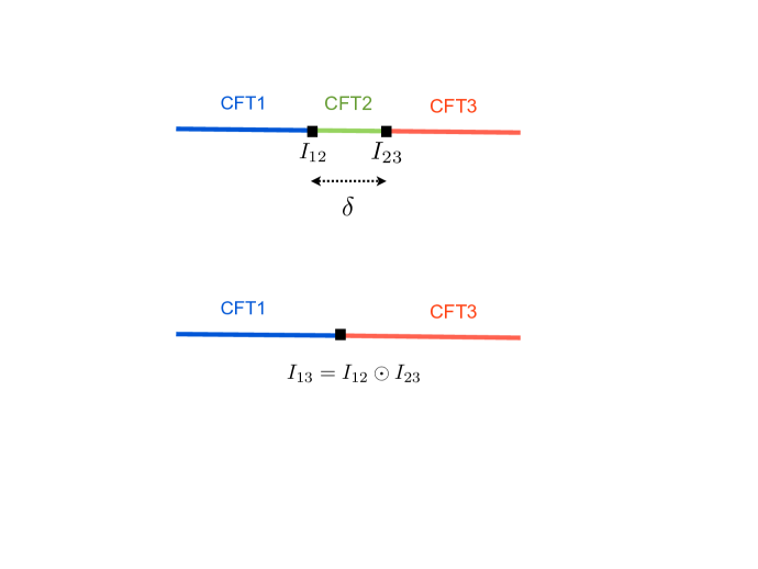
Figure 1: The fusion of two interfaces corresponds to taking the size, $\delta$, of the middle region to zero. Only the $\tau$ axis is drawn in the figure. The $\sigma$ coordinate parametrizes either a circular space, or a periodic Euclidean time.

On the level of classical gluing conditions fusion amounts to multiplication of $O(1,1|\mathbb{R})$ matrices. Indeed, let $\Lambda$ and $\Lambda^{\prime}$ be the gluing matrices for the left and right $\widehat{u}(1)$ currents imposed by the interfaces $I_{23}$ and $I_{12}$, so that

$$\left(\begin{array}[]{c}a_{n}^{1}\\ -\tilde{a}_{-n}^{1}\end{array}\right)\,=\,\Lambda^{\prime}\left(\begin{array}[]{c}a_{n}^{2}\\ -\tilde{a}_{-n}^{2}\end{array}\right)\Bigl{|}_{\tau=\delta}\ \ \ {\rm and}\ \ \ \left(\begin{array}[]{c}a_{n}^{2}\\ -\tilde{a}_{-n}^{2}\end{array}\right)\,=\,\Lambda\left(\begin{array}[]{c}a_{n}^{3}\\ -\tilde{a}_{-n}^{3}\end{array}\right)\Bigl{|}_{\tau=0}\ .$$ (83)

Taking $\delta\to 0$ leads, by continuity, to the gluing condition

$$\left(\begin{array}[]{c}a_{n}^{1}\\ -\tilde{a}_{-n}^{1}\end{array}\right)\,=\,\Lambda^{\prime}\Lambda\left(\begin{array}[]{c}a_{n}^{3}\\ -\tilde{a}_{-n}^{3}\end{array}\right)\Bigl{|}_{\tau=\delta=0}\ .$$ (84)

Likewise for the fermions, fusion leads to the gluing condition

$$\left(\begin{array}[]{c}\psi^{1}_{r}\\ -i\eta_{\rm S}^{1}\,\tilde{\psi}^{1}_{-r}\end{array}\right)\,=\,\eta^{\prime}\eta\,\Lambda^{\prime}\Lambda\left(\begin{array}[]{c}\psi^{3}_{r}\\ -i\eta_{\rm S}^{3}\,\tilde{\psi}^{3}_{-r}\end{array}\right)\Bigl{|}_{\tau=\delta=0}\ ,$$ (85)

provided the two interfaces preserve the same supersymmetry in the middle region, so that the factors of $\eta_{S}^{2}$ cancel out, c.f. equations (51) and (52). In the sequel we will always assume this to be the case.

In the quantum theory, fusion is defined by the composition of interface operators, which, as alluded to above, requires regularization. One defines

$$I_{12}\odot I_{23}\,:=\,{\rm lim}_{\delta\to 0}\,{\cal R}_{\delta}[I_{12}\,e^{-\delta H}I_{23}]\,,$$ (86)

where $H\equiv L_{0}+\tilde{L}_{0}$ is the Hamiltonian of CFT2. (We drop the -${c\over 12}$ term which commutes with the interface operators and therefore does not contribute to our analysis.) ${\cal R}_{\delta}$ denotes the renormalization procedure which, by the usual arguments of quantum field theory, can be achieved by local counterterms. For the superconformal interfaces we study here, fusion turns out to be finite without renormalization, so that the symbol ${\cal R}_{\delta}$ can be omitted.

Although the gluing conditions still compose according to multiplication in $O(1,1|\mathbb{R})$, fusion of the quantum interfaces is much more subtle. Firstly, as we have seen in Section 2, the quantization of the $u(1)$ charges restricts the gluing matrices to lie in dense subsets of $O(1,1|\mathbb{R})$ which are isomorphic to the rational subgroup $O(1,1|\mathbb{Q})$. Furthermore, in order to respect charge quantization the interface operators have to project to sublattices of the charge lattice, while the remaining sectors are projected out. If this sublattice is a proper sublattice, the respective interface is not invertible. As a result, the classical $O(1,1|\mathbb{R})$ group is replaced in the quantum theory by a semi-group. Moreover, quantum interfaces can be superposed, i.e. the associated operators are added. In particular the superposition of interfaces with different values of the classically irrelevant moduli $\varphi$ can give rise to non-trivial effects.

For all these reasons the algebraic structure of quantum interfaces is richer and more interesting than that of their classical counterparts. This will be discussed in the rest of this paper.

4.2 Intertwiners for non-zero modes

We will perform the fusion (86) of the superconformal interfaces by separately composing the bosonic and fermionic interface operators. According to (22) and (70), these latter can be written as tensor products of maps on the different frequency sectors of the (free) CFTs:

$$I_{1,2}=\prod_{n>0}I_{1,2}^{n}\,I_{1,2}^{0}\equiv I_{1,2}^{>}I_{1,2}^{0}\,.$$ (87)

As derived in Section 3 the $I_{1,2}^{n}$ for $n>0$ can be expressed as exponentials of quadratic expressions of the bosonic, respectively fermionic, modes, c.f. (20) and (65). We recall that operators of CFT1 act on the zero-mode part from the left while the operators of CFT2 act from the right.

In order to obtain (86), we first calculate $I_{1,2}^{n}e^{-\delta H}I_{2,3}^{n}$ for the tensor factors. The bosonic expressions can be evaluated along the lines of [9]. Pushing the Hamiltonian in the product $I_{1,2}^{\,n,{\rm bos}}e^{-\delta H}I_{2,3}^{\,n,{\rm bos}}$ to the left multiplies the oscillators $a^{2}_{n}$ and $\tilde{a}^{2}_{n}$ in $I_{1,2}^{\,n,{\rm bos}}$ by a factor $e^{-\delta n}$. Furthermore, the oscillators of CFT1 and CFT3 commute with every other operator in this calculation, and can be treated as c-numbers. This leaves us with the ground state matrix element of exponentials that are either linear or quadratic in the oscillators of CFT2. The identity

$${\rm exp}\,\left({1\over n}va_{n}\right)\,f(a_{-n})\,=\,f(a_{-n}+v)\,{\rm exp}\,\left({1\over n}va_{n}\right)\ ,$$ (88)

valid for any analytic function $f$ and any commuting operator $v$, allows us to push to the right in the matrix element all linear exponentials. We can then rearrange the quadratic terms with the use of the identity

$$\langle 0|\ {\rm exp}\,\left({1\over n}a_{n}M^{\prime}\,\tilde{a}_{n}\right)\,{\rm exp}\,\left({1\over n}a_{-n}M\,\tilde{a}_{-n}\right)$$

$$=\langle 0|\ {\rm det}(1-M^{\prime}M^{T})^{-1}\,{\rm exp}\left({1\over n}a_{n}(1-M^{\prime}M^{T})^{-1}M^{\prime}\,\tilde{a}_{n}\right)\ .$$ (89)

Finally, pushing the ensuing quadratic exponential through the linear terms on its right, and doing some straightforward algebra, leads to the following result for the product:

$$I_{1,2}^{\,n,{\rm bos}}(\mathcal{O}^{\prime})e^{-\delta H}I_{2,3}^{\,n,{\rm bos}}(\mathcal{O})={\rm det}(1-e^{-2n\delta}\mathcal{O}_{11}\mathcal{O}_{22}^{\prime})^{-1}\,I_{1,3}^{\,n,{\rm bos}}(\mathcal{O}^{\prime\prime}(e^{-\delta n}))\ ,$$ (90)

with

$${\scriptsize\mathcal{O}^{\prime\prime}(x)=\left(\begin{array}[]{cc}\mathcal{O}{}^{\prime}_{11}+x^{2}\mathcal{O}{}^{\prime}_{12}(1-x^{2}\mathcal{O}_{11}\mathcal{O}{}^{\prime}_{22})^{-1}\mathcal{O}_{11}\mathcal{O}{}^{\prime}_{21}&x\mathcal{O}{}^{\prime}_{12}(1-x^{2}\mathcal{O}_{11}\mathcal{O}{}^{\prime}_{22})^{-1}\mathcal{O}_{12}\\ x\mathcal{O}_{21}(1-x^{2}\mathcal{O}{}^{\prime}_{22}\mathcal{O}_{11})^{-1}\mathcal{O}{}^{\prime}_{21}&\mathcal{O}_{22}+x^{2}\mathcal{O}_{21}(1-x^{2}\mathcal{O}{}^{\prime}_{22}\mathcal{O}_{11})^{-1}\mathcal{O}{}^{\prime}_{22}\mathcal{O}_{12}\end{array}\right)\,.}$$ (91)

Collecting all the positive-frequency contributions of the bosonic intertwiners to (86) we obtain

$$I_{1,2}^{>,{\rm bos}}(\mathcal{O}{}^{\prime})e^{-\delta H}I_{2,3}^{>,{\rm bos}}(\mathcal{O})=\prod_{n>0}\det(1-e^{-2\delta n}\mathcal{O}_{11}\mathcal{O}{}^{\prime}_{22})^{-1}I_{1,3}^{n,\rm bos}(\mathcal{O}^{\prime\prime}(e^{-\delta n}))\,.$$ (92)

In the limit $\delta\to 0$ the matrices $\mathcal{O}^{\prime\prime}(e^{-\delta n})$ converge to the orthogonal matrix associated via (10) to the product of the gluing conditions $\Lambda{}^{\prime}$ and $\Lambda$,

$$\mathcal{O}^{\prime\prime}(e^{-\delta n})\stackrel{{\scriptstyle\delta\to 0}}{{\longrightarrow}}\mathcal{O}(\Lambda{}^{\prime}\Lambda)\ .$$ (93)

The product of determinants, on the other hand, exhibits a singular behavior in this limit due to a divergent Casimir energy [9].

Repeating the calculation for the fermionic intertwiners yields

$$I_{1,2}^{\,r,{\rm ferm}}(\mathcal{O}^{\prime})e^{-\delta H}I_{2,3}^{\,r,{\rm ferm}}(\mathcal{O})={\rm det}(1-e^{-2r\delta}\mathcal{O}_{11}\mathcal{O}_{22}^{\prime})\,I_{1,3}^{\,r,{\rm ferm}}({\mathcal{O}}^{\prime\prime}(e^{-\delta r}))\ ,$$ (94)

which combines to

$$I_{1,2}^{>,{\rm ferm}}(\mathcal{O}{}^{\prime})e^{-\delta H}I_{2,3}^{>,{\rm ferm}}(\mathcal{O})=\prod_{r>0}\det(1-e^{-2\delta r}\mathcal{O}_{11}\mathcal{O}{}^{\prime}_{22})I_{1,3}^{r,\rm ferm}(\mathcal{O}^{\prime\prime}(e^{-\delta r}))\$$ (95)

for the positive-frequency contributions to the fusion (86). The useful fermionic identities, analogous to (88) and (89), are

$${\rm exp}\,(\chi\psi_{r})\,f(\psi_{-r})\,=\,f(\psi_{-r}+\chi)\,{\rm exp}\,(\chi\psi_{r})$$ (96)

for $\chi$ an operator anticommuting with the fermionic oscillators, and

$$\langle 0|\ {\rm exp}\,(\psi_{r}M^{\prime}\,\tilde{\psi}_{r})\,{\rm exp}\,(\psi_{-r}M\,\tilde{\psi}_{-r})$$

$$=\langle 0|\ {\rm det}(1-M^{\prime}M^{T})\,{\rm exp}\left(\psi_{r}(1-M^{\prime}M^{T})^{-1}M^{\prime}\,\tilde{\psi}_{r}\right)\ .$$ (97)

Note that the determinant factors in expression (95) appear with opposite exponent as the ones in the corresponding bosonic formula (92).

When composing two superconformal interfaces, one should replace the matrices $\mathcal{O}{}^{\prime}$ and $\mathcal{O}$ in the expression (95) by the fermion-gluing matrices $\mathcal{O}{}^{\prime}_{\rm F}$ and $\mathcal{O}_{\rm F}$. Nevertheless, the determinant that enters in the formulae for the bosons and fermions is the same. Indeed, let $(\eta{}^{\prime},\eta_{\rm S}^{1},\eta_{\rm S}^{2})$ be the signs associated with $I_{12}$, and $(\eta,\eta_{\rm S}^{2},\eta_{\rm S}^{3})$ those associated with $I_{23}$, c.f. (51). Then from (10) we find:

$$\mathcal{O}_{\rm F}\equiv\mathcal{O}(\Lambda_{\rm F})=\left(\begin{array}[]{cc}\eta_{\rm S}^{2}\,\Lambda_{12}\Lambda_{22}^{-1}&\eta\,\Lambda_{11}-\eta\,\Lambda_{12}\Lambda_{22}^{-1}\Lambda_{21}\\ \eta\eta_{\rm S}^{2}\eta_{\rm S}^{3}\,\Lambda_{22}^{-1}&-\eta_{\rm S}^{3}\,\Lambda_{22}^{-1}\Lambda_{21}\end{array}\right)\,,$$ (98)

and

$$\mathcal{O}{}^{\prime}_{\rm F}\equiv\mathcal{O}(\Lambda{}^{\prime}_{\rm F})=\left(\begin{array}[]{cc}\eta_{\rm S}^{1}\,\Lambda{}^{\prime}_{12}(\Lambda{}^{\prime}_{22})^{-1}&\eta{}^{\prime}\,\Lambda{}^{\prime}_{11}-\eta{}^{\prime}\,\Lambda{}^{\prime}_{12}(\Lambda{}^{\prime}_{22})^{-1}\Lambda{}^{\prime}_{21}\\ \eta{}^{\prime}\eta_{\rm S}^{1}\eta_{\rm S}^{2}\,(\Lambda{}^{\prime}_{22})^{-1}&-\eta_{\rm S}^{2}\,(\Lambda{}^{\prime}_{22})^{-1}\Lambda{}^{\prime}_{21}\end{array}\right)\,.$$ (99)

It follows from these expressions that $(\mathcal{O}_{\rm F})_{11}(\mathcal{O}{}^{\prime}_{\rm F})_{22}=\mathcal{O}_{11}\mathcal{O}{}^{\prime}_{22}$, i.e. all the supersymmetry-related signs cancel in this particular combination. Crucial for this to happen is the assumption that the interfaces preserve the same supersymmetry in the CFT2 region between them, i.e. that the same sign $\eta_{\rm S}^{2}$ is chosen for both $I_{12}$ and $I_{23}$.

Let us finally put together all the positive-mode bosonic and fermionic intertwiners

$$I_{1,2}^{>}=I_{1,2}^{>,{\rm bos}}\otimes I_{1,2}^{>,{\rm ferm}}\,.$$ (100)

In the Ramond sector, where the fermionic-mode frequencies $r$ are integer, the determinant factors in (95) exactly cancel the ones from the bosonic intertwiners (92). Thus, one can take the limit $\delta\to 0$ to obtain

$$I_{1,2}^{>}(\Lambda{}^{\prime},\eta{}^{\prime},\eta_{S}^{1},\eta_{S}^{2})\,I_{2,3}^{>}(\Lambda,\eta,\eta_{S}^{2},\eta_{S}^{3})=I_{1,3}^{>}(\Lambda{}^{\prime}\Lambda,\eta\eta{}^{\prime},\eta_{S}^{1},\eta_{S}^{3})\quad{\rm R\,\,sector}\,.$$ (101)

In the NS sector, on the other hand, the $r$ are half integers, and the determinant factor from the bosonic sector is not cancelled by the one from the fermionic sector. However, its singular behavior for $\delta\to 0$ does cancel. This can be seen with the help of the Euler-Maclaurin formula, which implies

$${\rm lim}_{\delta\to 0}\,\sum_{n\geq 1}F(e^{-2\delta n})={1\over\delta}\int_{0}^{\infty}dx\,F(e^{-2x})-{1\over 2}F(1)+{\delta\over 6}F^{\prime}(1)+O(\delta^{2})\ ,$$

$${\rm lim}_{\delta\to 0}\,\sum_{n\geq 1}F(e^{-2\delta n+\delta})={1\over\delta}\int_{0}^{\infty}dx\,F(e^{-2x})-{\delta\over 12}F^{\prime}(1)+O(\delta^{2})\ .$$ (102)

for any function $F$ vanishing analytically at the origin. Substituting $F(z)\equiv{\ln\,\det}(1-z\mathcal{O}_{11}\mathcal{O}_{22}^{\prime})$ one finds

$$I_{1,2}^{>}(\Lambda{}^{\prime},\eta{}^{\prime},\eta_{S}^{1},\eta_{S}^{2})\,I_{2,3}^{>}(\Lambda,\eta,\eta_{S}^{2},\eta_{S}^{3})=$$ (103)

$$\qquad\qquad\qquad\sqrt{\det(1-\mathcal{O}_{11}\mathcal{O}{}^{\prime}_{22})}\,I_{1,3}^{>}\,(\Lambda{}^{\prime}\Lambda,\eta{}^{\prime}\eta,\eta_{S}^{1},\eta_{S}^{3})\quad{\rm NS\,\,sector}\,.$$

The NS fermions precisely cancel the divergent Casimir energy of the bosons. The final answer for the composition of oscillator intertwiners in the NS sector is identical to the renormalized one in the purely bosonic model [9].

4.3 Zero modes and the defect monoid

It follows from (101) and (103) that the composition of positive-frequency parts of the interface operators is consistent with the one in the classical theory, which is given by group multiplication. In other words, if $(\Lambda,\eta)$ and $(\Lambda{}^{\prime},\eta{}^{\prime})$ are the data that determine the positive-frequency parts $I^{>}_{2,3}$ and $I^{>}_{1,2}$, then the data in the positive-frequency part of $I_{1,3}=I_{1,2}\odot I_{2,3}$ is $(\Lambda{}^{\prime}\Lambda,\eta{}^{\prime}\eta)$. The only subtlety is the appearance of the determinant in the NS sector. As we will see, this is precisely what is needed in order for the $g$-factors to compose as they should.

Consider first the unprojected theory, where the interface operators are those given in (71). The identity maps (66) between NS-fermion ground states compose trivially,

$$I_{1,2}^{0,{\rm NS}}I_{2,3}^{0,{\rm NS}}=I_{1,3}^{0,{\rm NS}}\,.$$ (104)

To complete the calculation of (86) we therefore only have to compose the bosonic ground state maps (32). A simple calculation gives

$$I_{1,2}^{0,{\rm bos}}I_{2,3}^{0,{\rm bos}} = {\left(g(\Lambda{}^{\prime})\sum_{\hat{\gamma}{}^{\prime}\in\mathbb{Z}^{1,1}}e^{2\pi i\varphi{}^{\prime}(\hat{\gamma}{}^{\prime})}|\hat{\Lambda}{}^{\prime}\hat{\gamma}{}^{\prime}\rangle\langle\hat{\gamma}{}^{\prime}|\,\Pi_{\hat{\Lambda}{}^{\prime}}\right)\left(g(\Lambda)\sum_{\hat{\gamma}\in\mathbb{Z}^{1,1}}e^{2\pi i\varphi(\hat{\gamma})}|\hat{\Lambda}\hat{\gamma}\rangle\langle\hat{\gamma}|\,\Pi_{\hat{\Lambda}}\right)}$$ (105)

$$= g(\Lambda{}^{\prime})g(\Lambda)\,\sum_{\hat{\gamma}\in\mathbb{Z}^{1,1}}e^{2\pi i[\varphi{}^{\prime}(\hat{\Lambda}\hat{\gamma})+\varphi(\hat{\gamma})]}\,|\hat{\Lambda}{}^{\prime}\hat{\Lambda}\hat{\gamma}\rangle\langle\hat{\gamma}|\,\Pi_{\hat{\Lambda}{}^{\prime}\hat{\Lambda}}\Pi_{\hat{\Lambda}}\ ,$$

where $g(\Lambda)=\sqrt{{\rm ind}(\hat{\Lambda})|\Lambda_{22}|}\$ is the $g$-factor of the interface. The result looks like the ground state map for an interface with gluing matrix $\Lambda^{\prime}\Lambda$, except for two important differences: (i) in general $g(\Lambda{}^{\prime})g(\Lambda)\not=g(\Lambda^{\prime}\Lambda)$, and (ii) there is an extra projector, $\Pi_{\hat{\Lambda}}$, in addition to the projector $\Pi_{\hat{\Lambda}{}^{\prime}\hat{\Lambda}}$.

Concerning the normalization, note that the product of $g$-factors should be multiplied by the determinant from the composition of the positive-frequency parts, c.f. equation (103). In the case at hand from (12) and (13) we find $\mathcal{O}_{11}={\rm tanh}\alpha$ and $\mathcal{O}_{22}^{\prime}=\varepsilon{}^{\prime}{\rm tanh}\alpha^{\prime}$, so that the product of the determinant and of the two $g$-factors yields

$$\sqrt{\det(1-\mathcal{O}_{11}\mathcal{O}{}^{\prime}_{22})}\,g(\Lambda{}^{\prime})g(\Lambda)$$ (106)

$$\qquad=\sqrt{|k{}^{\prime}_{1}k{}^{\prime}_{2}k_{1}k_{2}|}\sqrt{(1+\varepsilon{}^{\prime}{\rm tanh}\alpha{}^{\prime}{\rm tanh}\alpha)({\rm cosh}\alpha{}^{\prime}{\rm cosh}\alpha)}$$

$$\qquad=\sqrt{|k{}^{\prime}_{1}k{}^{\prime}_{2}k_{1}k_{2}|}\sqrt{{\rm cosh}(\alpha+\varepsilon{}^{\prime}\alpha{}^{\prime})}=\sqrt{{|k{}^{\prime}_{1}k{}^{\prime}_{2}k_{1}k_{2}|\over{\rm ind}(\hat{\Lambda}{}^{\prime}{}^{\prime})}}g(\Lambda{}^{\prime}{}^{\prime})\,.$$

In the last step, we used that ${\rm cosh}(\alpha+\varepsilon{}^{\prime}\alpha{}^{\prime})=|\Lambda^{\prime\prime}_{22}|$ where $\Lambda^{\prime\prime}=\Lambda^{\prime}\Lambda$. Thus, if ${\rm ind}(\hat{\Lambda}^{\prime\prime})$ were equal to $|k{}^{\prime}_{1}k{}^{\prime}_{2}k_{1}k_{2}|$, we would precisely obtain $g(\Lambda^{\prime\prime})$, i.e. the $g$-factor of an elementary interface with gluing matrix $\Lambda^{\prime\prime}$.

In general, however, ${\rm ind}(\hat{\Lambda}^{\prime\prime})\not=|k{}^{\prime}_{1}k{}^{\prime}_{2}k_{1}k_{2}|$ so that the fusion of two simple interfaces is not a simple interface, but rather the sum of several simple interfaces. To see this let for example $\Lambda{}^{\prime}=\Lambda^{-1}$, so that the composition of gluing matrices is the identity matrix, $\Lambda^{\prime\prime}={\bf 1}$. Let also CFT1 and CFT3 be the same conformal theory, so that the interface $I_{1,2}$ is the “would-be inverse” of the interface $I_{2,3}$. Clearly, in this case $k{}^{\prime}_{1}/k{}^{\prime}_{2}=k_{2}/k_{1}$ since $\hat{\Lambda}{}^{\prime}$ is the inverse of $\hat{\Lambda}$. For simplicity we set $\varphi{}^{\prime}=\varphi=0$. The ground state map (105) multiplied by the determinant from the positive-frequency modes then gives

$$|k_{1}k_{2}|\,\Pi_{\hat{\Lambda}}=\sum_{N,M}\sum_{n,m=0}^{k_{1},k_{2}}e^{2\pi i({Nn\over k_{1}}+{Mm\over k_{2}})}|N,M\rangle\langle N,M|\ ,$$ (107)

i.e. the sum of $|k_{1}k_{2}|$ identity interfaces, with phase moduli arranged in a periodic array so as to implement the projection on the charge sublattice $k_{1}\mathbb{Z}\oplus k_{2}\mathbb{Z}$. Only for $|k_{1}|=|k_{2}|=1$, i.e. if $\hat{\Lambda}\in O(1,1|\mathbb{Z})$, does fusion yield the identity interface. For all other $\hat{\Lambda}\in O(1,1|\mathbb{Q})$ the projector is non-trivial, and the corresponding interface operators cannot be inverted.

The algebraic structure of $\widehat{u}(1)^{2}$ preserving interfaces in the unprojected-fermion theory is the same as in the purely bosonic theory [9, 8], modulo a $\mathbb{Z}_{2}$ that changes the sign of the fermion field. To describe this algebraic structure, we first note that two interfaces can only be added if they separate the same CFTs. They can only be fused if the CFT to the right of the first interface is the same as the CFT to the left of the second interface. These conditions are automatically obeyed if we restrict attention to interfaces between identical CFTs. We will call such interfaces “defect lines”. Two defects in the same CFT can be always added and fused, and fusion is distributive over addition. If we also allowed subtraction, these defects would form a ring. But subtraction is not a physical operation since negative $g$-factors correspond to imaginary entropy. So the set of defects is a monoid (or semi-group) with respect to both, addition and fusion.

The monoid of conformal defect lines is independent of the continuous moduli of the underlying CFT. This can be seen by fusing from both left and right with special invertible interfaces (called “deformed identities” in [9]) which parallel transport the CFT along the connected components of its moduli space [25]. In the case at hand, these are the interfaces with $\hat{\Lambda}={\bf 1}$, $\varphi=0$ and $\eta=1$ in the notation of Section 2.2.

Any $\widehat{u}(1)^{2}$ preserving interface between circle theories can in this way be converted to a $\widehat{u}(1)^{2}$ preserving defect line in any given circle theory. Since this latter is irrelevant for the algebraic structure of the defects, we do not have to indicate it explicitly. We therefore parametrize the simple defects by $(\hat{\Lambda},\varphi,\eta)$, where the gluing matrix $\hat{\Lambda}\in O(1,1|\mathbb{Q})$.

The fusion of any two defects can always be written as the sum of simple defects. The rule for two simple defects reads

$$(\hat{\Lambda}{}^{\prime},\varphi{}^{\prime},\eta{}^{\prime})\odot(\hat{\Lambda},\varphi,\eta)=\sum_{\varphi^{\prime\prime}}\,(\hat{\Lambda}{}^{\prime}\hat{\Lambda},\varphi^{\prime\prime},\eta{}^{\prime}\eta)\,,$$ (108)

where the sum runs over an array of $K$ linear forms on the sublattice that is projected out by $\Pi_{\hat{\Lambda}{}^{\prime}\hat{\Lambda}}$. These forms have the following property: their exponentials are independent functions which, when restricted to the (in general smaller) sublattice projected out by $\Pi_{\hat{\Lambda}{}^{\prime}\hat{\Lambda}}\Pi_{\hat{\Lambda}}$ obey

$$e^{2\pi i{\varphi^{\prime\prime}}(\hat{\gamma})}=e^{2\pi i{\varphi{}^{\prime}}(\hat{\Lambda}\hat{\gamma})+\varphi(\hat{\gamma})}\qquad{\rm when}\ \ \ \Pi_{\hat{\Lambda}{}^{\prime}\hat{\Lambda}}\Pi_{\hat{\Lambda}}|\hat{\gamma}\rangle=|\hat{\gamma}\rangle\ .$$ (109)

If we parametrize the matrices as in (27), with $(k_{1},k_{2})$ and $(k{}^{\prime}_{1},k{}^{\prime}_{2})$ coprime integers, then the number $K$ of terms in the sum is given by

$$K=\left\{\begin{array}[]{cc}{\rm gcd}(k_{1}k{}^{\prime}_{1},k_{2}k{}^{\prime}_{2})\,,&{\rm det}\hat{\Lambda}=1\ ,\\ {\rm gcd}(k_{1}k{}^{\prime}_{2},k_{2}k{}^{\prime}_{1})\,,&{\rm det}\hat{\Lambda}=-1\ .\end{array}\right.$$ (112)

The above rules determine completely the $\widehat{u}(1)^{2}$ preserving defect monoid in the non-GSO projected theories.

Consider next the GSO projected theories. Instead of the fermion sign $\eta$, elementary interfaces are now characterized by their R charge: they can have charge $\pm$ or be neutral, c.f. expressions (79), (80) and (81). As discussed in Section 3.3, an interface is charged if $\zeta\det\hat{\Lambda}=\zeta\det\Lambda=+1$ and it is neutral if $\zeta\det\Lambda=-1$, where $\zeta=\pm 1$ distinguishes whether the GSO projections on both sides of the interface are taken to be the same ($+1$) or opposite ($-1$). If we insist that the GSO projection on both sides be the same, i.e. $\zeta=1$, then the choice of $\hat{\Lambda}$ and the R charge are correlated.

When fusing the projected interfaces, one has to compose separately the NS and the R components of the interface operators. In the NS sector, the calculation only differs from the one in the unprojected theories by an additional normalization factor ${1/2}$ for the charged interfaces and ${1/\sqrt{2}}$ for the neutral ones. For simplicity, we suppress the dependence on phase moduli $\varphi$, which is the same as in (108). Fusion of the NS components can be described by the following rules:

$$(\hat{\Lambda}{}^{\prime},{\rm charge}\,\pm)\odot(\hat{\Lambda},{\rm neutral})=(\hat{\Lambda}{}^{\prime},{\rm neutral})\odot(\hat{\Lambda},{\rm charge}\,\pm)=K(\hat{\Lambda}{}^{\prime}\hat{\Lambda},{\rm neutral})\,,$$

$$(\hat{\Lambda}{}^{\prime},{\rm neutral})\odot(\hat{\Lambda},{\rm neutral})=K\left[(\hat{\Lambda}{}^{\prime}\hat{\Lambda},{\rm charge}\,+)+(\hat{\Lambda}{}^{\prime}\hat{\Lambda},{\rm charge}\,-)\right]\ ,$$

$$(\hat{\Lambda}{}^{\prime},{\rm charge}\,s{}^{\prime})\odot(\hat{\Lambda},{\rm charge}\,s)=K(\hat{\Lambda}{}^{\prime}\hat{\Lambda},{\rm charge}\,ss{}^{\prime})\,.$$ (113)

Here $K$ is the number of elementary defects with phase moduli in an appropriate array, as discussed for the unprojected theory above.

Note that only in the third line do the R sectors actually contribute to the fusion product. The neutral operators in the second line have of course no R-sector terms, consistently with the fact that on the right-hand-side of the equation one sums over interfaces with opposite R charge, so that the R-sector operators precisely cancel.

To verify that the R-sector operators compose as in the third line of (113), recall the expression (67) for the ground state maps, and the expression for the defect $g$-factor (which can be found in (21)). Combining these two expressions one finds

$$g(\Lambda{}^{\prime})I_{1,2}^{0,{\rm R}}(\Lambda{}^{\prime})\,g(\Lambda)I_{2,3}^{0,{\rm R}}(\Lambda)=\sqrt{|k_{1}k_{2}k{}^{\prime}_{1}k{}^{\prime}_{2}|}\,\imath^{\rm R}_{1,3}\,S(\Lambda{}^{\prime}\Lambda)$$

$$=\,K\,g(\Lambda{}^{\prime}\Lambda)\,I_{1,3}^{0,{\rm R}}(\Lambda{}^{\prime}\Lambda)\ .$$ (114)

Recall furthermore that there is no determinant from the positive-frequency modes in the R sector, where the bosonic contribution exactly cancels the contribution of fermions. Finally, $I_{1,2}^{{\rm R}}$ has a coefficient $1/2$ in the full expression (80) for the interface operator, and we must sum over the two possible values of $\eta$. Putting all these facts together one finds that the R-sector operators compose indeed as indicated in the third line of (113).

The $\widehat{u}(1)^{2}$ preserving defect algebra in the GSO projected $c=3/2$ theory can be described more succinctly as follows: it is the tensor product of the $\widehat{u}(1)^{2}$ preserving defect algebra in the bosonic $c=1$ theory, tensored with the fusion algebra of the Ising model. The latter reads

$$\epsilon\times\epsilon=1\ ,\qquad\epsilon\times\sigma=\sigma\ ,\qquad\sigma\times\sigma=1+\epsilon\ .$$ (115)

Identifying $1$ and $\epsilon$ with the two charged interfaces, and $\sigma$ with the neutral interface, reproduces precisely the pattern (113) in the fermion sector.

This is not a coincidence. The conformal defects of the Ising model, analyzed in [21, 2, 5, 23], can be described in our language by the data $(\Lambda,\alpha)_{\rm Ising}$, where $\alpha\in\{1,\epsilon,\sigma\}$ labels the R charge in the way just described, $\Lambda$ and $-\Lambda$ correspond to identical defects, and ${\rm det}\Lambda=+1$ for charged defects and $-1$ for the neutral ones. One may compute the fusion of these defects, without associating them necessarily to the bosonic field, by subtracting the divergent Casimir energies as in [9]. The result is

$$(\Lambda{}^{\prime},\alpha{}^{\prime})_{\rm Ising}\odot(\Lambda,\alpha)_{\rm Ising}=(\Lambda{}^{\prime}\Lambda,\alpha{}^{\prime}\times\alpha)_{\rm Ising}\ ,$$ (116)

where $\alpha{}^{\prime}\times\alpha$ is given by (115) and the sum of Ising primaries indicates in the above equation the sum of the corresponding interface operators.

The defect $(\Lambda,\alpha)_{\rm Ising}$ is topological if and only if $\Lambda\in O(1)\times O(1)$. The topological defects of the Ising model are known to be in one-to-one correspondence with primary fields, and their fusion algebra is the Verlinde algebra [2]. This provides a consistency check of the more general analysis presented here.

5 Topological interfaces as quasi-symmetries

The defects described in the previous sections are specified by the following data: the moduli of the bulk CFT, i.e. a radius $R_{1}=R_{2}$, the gluing matrix $\hat{\Lambda}\in O(1,1|\mathbb{Q})$ of the integer charges, and the phase moduli $\varphi$. Furthermore the fermionic gluing conditions require some extra data: the sign $\eta=\pm 1$ in the unprojected theory, and in the GSO projected theory, the Ramond charge ($\pm$, or neutral), or equivalently an Ising primary ($1,\sigma,\epsilon$). Again, we fix the preserved supersymmetry algebras by setting $\eta_{\rm S}^{j}=1$. The gluing matrix for the fermion fields is thus given by $\eta\Lambda$, where $\Lambda=U_{2}\hat{\Lambda}U_{2}^{-1}$ is the gluing matrix for bosonic currents.

These defects are superconformal and preserve a $\widehat{u}(1)^{2}$ current algebra. Generically, they are not topological. However, as explained in Section 2.2, for any such defect $I_{R_{2},R_{2}}(\hat{\Lambda},\varphi)$, there is a unique radius $R_{1}=f_{\hat{\Lambda}}(R_{2})$ such that parallel transport yields a topological interface between the theories of radius $R_{2}$ and $R_{1}$. Explicitly $I_{R_{1},R_{2}}(\hat{\Lambda},\varphi)=D_{R_{1},R_{2}}\odot I_{R_{2},R_{2}}(\hat{\Lambda},\varphi)$ where $D_{R_{1},R_{2}}$ is the deformed identity interface that transports the theory from $R_{2}$ to $R_{1}=f_{\hat{\Lambda}}(R_{2})$, c.f. the previous subsection. In fact, this was only explained for the bosonic components, but due to supersymmetry, it immediately carries over to the fermions as well.

Since $R_{2}$ is arbitrary, parallel transport indeed yields an isomorphism between the fusion algebra of $\widehat{u}(1)^{2}$-preserving conformal defect lines in any given circle theory (they are all isomorphic), and the fusion algebra of $\widehat{u}(1)^{2}$-preserving topological interfaces between circle theories. To be more precise, for any radius $R_{3}$, and any gluing matrices $\hat{\Lambda}{}^{\prime},\hat{\Lambda}$ there are radii $R_{2}=f_{\hat{\Lambda}}(R_{3})$ and $R_{1}=f_{\hat{\Lambda}{}^{\prime}}(R_{2})$ such that the interfaces $I_{R_{1},R_{2}}(\hat{\Lambda}{}^{\prime},\varphi{}^{\prime})$ and $I_{R_{2},R_{3}}(\hat{\Lambda},\varphi)$ are topological and their fusion is given by parallel transport of the fusion of the respective conformal defects in the theory with radius $R_{3}$:

$$I_{R_{1},R_{2}}(\hat{\Lambda}{}^{\prime},\varphi{}^{\prime})\odot I_{R_{2},R_{3}}(\hat{\Lambda},\varphi)=D_{R_{1},R_{3}}\odot I_{R_{3},R_{3}}(\hat{\Lambda}{}^{\prime},\varphi{}^{\prime})\odot I_{R_{3},R_{3}}(\hat{\Lambda},\varphi)\,.$$ (117)

[We have suppressed the fermion-interface labels for simplicity].

Thus, the monoids of $\widehat{u}(1)^{2}$-preserving conformal defects and topological interfaces in torus models are isomorphic. The isomorphism actually breaks down if the requirement of $\widehat{u}(1)^{2}$-symmetry is dropped. This would allow for example the addition of defects with different gluing conditions $\hat{\Lambda}$ and $\hat{\Lambda}{}^{\prime}$, but topological interfaces can only be added if the theories on both sides agree, i.e. if $f_{\hat{\Lambda}}(R)=f_{\hat{\Lambda}{}^{\prime}}(R)$.

In the next subsection, we will explain how the topological interfaces on the string worldsheet are related to the $O(1,1|\mathbb{R})$ symmetry of classical supergravity compactified on a circle.

5.1 Action on perturbative string states

Consider first the purely bosonic theory and let $\hat{\Lambda}$ be the gluing matrix for the integer charges. If the topological condition $R_{1}=f_{\hat{\Lambda}}(R_{2})$ is satisfied, the gluing condition $\Lambda=U_{1}^{-1}\hat{\Lambda}U_{2}\in O(1)\times O(1)=\{{\rm diag}(\pm 1,\pm 1)\}$, which implies that left and right Virasoro algebras commute separately with the interface operator.

In the following, we will restrict our attention to the case $\Lambda={\bf 1}$. The other cases can be obtained from this one by T-duality transformations, which are implemented by invertible topological interfaces with $\hat{\Lambda}\in O(1,1|\mathbb{Z})$. Since T-duality is well understood [1], we refrain from giving any more detail on these other cases here.

From the expressions (6) and (32) we deduce that the topological-interface operator maps states in CFT2 to states in CFT1 as follows:

$$(\prod_{\{n_{i}\}}a_{n_{i}}^{\dagger})(\prod_{\{\tilde{n}_{j}\}}\tilde{a}_{\tilde{n}_{j}}^{\dagger})|\hat{\gamma}\rangle\ \to\ e^{2\pi i\varphi(\hat{\gamma})}\,\sqrt{|k_{1}k_{2}|}\,(\prod_{\{n_{i}\}}a_{n_{i}}^{\dagger})(\prod_{\{\tilde{n}_{j}\}}\tilde{a}_{\tilde{n}_{j}}^{\dagger})|\hat{\Lambda}\hat{\gamma}\rangle$$ (118)

if $\hat{\gamma}\in k_{1}\mathbb{Z}\otimes k_{2}\mathbb{Z}$, while all other states are mapped to zero. Here we used that $\Lambda_{22}=1$ for $\Lambda={\bf 1}$.

The physical charge vector $\gamma:=U\hat{\gamma}$ is preserved by the above map,

$$U_{1}\hat{\Lambda}\hat{\gamma}=\Lambda(U_{2}\hat{\gamma})=U_{2}\hat{\gamma}\ ,$$ (119)

and hence, the masses

$${\cal M}_{\rm pert}^{2}=8\gamma^{T}\gamma+\sum_{i}2n_{i}+\sum_{j}\tilde{2}n_{j}\ .$$ (120)

of perturbative string states are also preserved. [Our convention is $\alpha^{\prime}=1/2$]. This of course is an immediate consequence of the property of topological interfaces to commute with left and right Virasoro algebras combined with the fact that masses of perturbative string states are proportional to $(L_{0}+\tilde{L}_{0})$.

In a nutshell, topological interfaces transform moduli and perturbative charges in the same way as the $O(d,d|\mathbb{R})$ symmetry of the low-energy action. But they have the ‘integrity’ to only transform charges if this is consistent with charge quantization. In fact, the transformations preserves a larger set of observables than the masses, as we will now explain.

Namely, any local operator $V$ with $u(1)$ charges $\hat{\gamma}\in k_{1}\mathbb{Z}\otimes k_{2}\mathbb{Z}$ is just multiplied by the factor $e^{2\pi i\varphi(\hat{\gamma})}\,\sqrt{|k_{1}k_{2}|}$ under the action of the interface operator. Thus, $N$-point correlation functions on the sphere transform by a common multiplicative factor,

$$\langle V_{1}V_{2}\cdots V_{N}\rangle_{\rm sphere}\ \mapsto\ |k_{1}k_{2}|^{N/2}\,\langle V_{1}V_{2}\cdots V_{N}\rangle_{\rm sphere}\ .$$ (121)

Note that the phase factors drop out from the expression on the right due to the $u(1)$-charge conservation.

Translated to string theory, (121) implies that the tree-level scattering amplitudes of states with vertex operators $V_{j}$ are invariant provided one also transforms the effective string coupling constant according to

$${\lambda_{c}\over\sqrt{2\pi R}}=:\lambda_{\rm eff}\ \mapsto\ \lambda_{\rm eff}\,\sqrt{|k_{1}k_{2}|}\ .$$ (122)

Here, $\lambda_{c}$ is the closed-string coupling constant in 26 dimensions, and $\lambda_{\rm eff}$ the effective coupling after compactification on a circle of radius $R$. This effective coupling can be defined as the common normalization of all vertex operators [42]. We stress that only a part of the tree-level S-matrix is preserved by the topological map, the part restricted to asymptotic states for which the $O(1,1|\mathbb{Q})$ transformation respects the charge quantization. All other string states are projected out.

The rescaling (122) of the coupling is surprising, because it depends on arithmetic properties of the $O(1,1|\mathbb{Q})$ gluing matrix. Since it amounts to a redefinition of the Planck scale, it is invisible classically, even if all stringy $\alpha{}^{\prime}$ corrections are included in the closed-string action. Nonetheless, it is crucial for the proper transformation of D-brane charges and masses.

Before proceeding to the treatment of D-branes, let us comment on a relation of our discussion with the orbifold construction. Indeed, since in the case at hand the quotient of the circle radii $R_{1}/R_{2}=k_{2}/k_{1}$ is rational, the theory with radius $R_{1}$ can be obtained from the one with radius $R_{2}$ by orbifolding with respect to the shift symmetry

$$\phi\to\phi+2\pi R_{1}\ .$$ (123)

The orbifold group generated by this symmetry is of order $k_{1}k_{2}$. The operator $\Pi_{\hat{\Lambda}}$ for $\hat{\Lambda}={\rm diag}({k_{2}/k_{1}},{k_{1}/k_{2}})$ projects on untwisted states of the orbifold, while all other states in CFT1 arise as twisted sectors.

This viewpoint demystifies the relations (121). These relations express the well-known fact that the parent and the orbifold theory share the same sphere amplitudes in the untwisted sector.

Indeed, our construction fits in nicely with the general framework of topological interfaces in rational CFTs put forward by Fröhlich et al [7]. These authors single out two classes of special topological interfaces in RCFT: (i) the so-called “group-like” interfaces, which describe automorphisms of CFTs, and which form a groupoid under fusion, and (ii) the broader class of “duality interfaces”, which have the property that fusion with their parity-transform results in a sum of group-like defects. It has been argued in [7] that duality interfaces exist between a parent theory and any of its orbifold descendants, and that such an interface is group-like only when the orbifold is the same CFT as the parent theory.

Although the arguments of [7] were made in the context of RCFT, they extend to the circle theories studied here. All the topological interfaces associated to gluing matrices $\hat{\Lambda}\in O(1,1|\mathbb{Q})$ are duality interfaces, whereas the ones with $\hat{\Lambda}\in O(1,1|\mathbb{Z})$ are group-like. The parent and orbifold theories of [7] are nothing but the theories at radius $R_{2}$, respectively $R_{1}$.

We may extend this analysis from the bosonic string theory to the type-0 or the type-II superstring theories in the following way. We first note that for a bosonic gluing matrix $\Lambda={\bf 1}$, the fermionic one is given by $\Lambda_{\rm F}=\pm{\bf 1}$, c.f. (51). Thus, left (right) fermions of CFT1 are glued to left (right) fermions of CFT2, i.e. the fermionic interface is automatically topological as well. This of course is a consequence of supersymmetry. The mass of the perturbative string states, which is still equal to the square root of $2(L_{0}+\tilde{L}_{0})$, is therefore still preserved by the interface map as in the purely bosonic case.

What needs to be checked is that the uniform rescaling (121) is also valid for states in the Ramond sector. We focus on charged interfaces, since the neutral ones anyway project out all Ramond states. Making use of $|{\rm sin}(2\vartheta)|=|\Lambda_{22}|=1$, and the property $S(\pm{\bf 1})=(\begin{smallmatrix}1&0\\ 0&\pm 1\end{smallmatrix})$ of the spinor representation, it follows from (67) that indeed all vertex operators transform with the same normalization factor.

This argument applies to the type-0 superstrings. The type-II superstring theory has separate GSO projections for the left- and right-moving fermion numbers. To implement these projections, we have to tensor the $c=3/2$ interfaces with the identity interface for the nine remaining non-compact dimensions. Because $\Lambda_{\rm F}=\pm{\bf 1}$, such topological interfaces commute or anticommute with $(-1)^{F}$ and $(-1)^{\tilde{F}}$. In the first case the interface must be resolved by the addition of new twisted contributions, which are intertwiners for the mixed R-NS sectors of the type-II theories. The construction proceeds along the lines described in Section 3.3. It is tedious but straightforward to check that for the ensuing topological interfaces, equation (121) still holds for states from all four sectors of the type-II superstring theory.

5.2 Action on D-branes

As alluded to above, interfaces not only transform perturbative string states, but also act on D-branes. This action is given by fusion with the respective boundary condition.

We consider (super)string theory compactified on a $d$-dimensional torus, and take any D-brane wrapped entirely around some of the torus directions, so that it looks like a point particle in the non-compact spacetime. The D-brane can be described by a boundary state $|{\cal B}\rangle\!\rangle$ of the $c=3d/2$ SCFT [we focus for definiteness on the type-0 supersymmetric case]. The mass of this point particle is proportional to the $g$-factor of the boundary state [43]

$${\cal M}_{\cal B}=\ 4(\sqrt{\pi})^{7-d}\,M_{\rm Planck}\,g_{\cal B}\ ,$$ (124)

where $M_{\rm Planck}$ is the Planck mass in the effective $(10-d)$ dimensional theory. It is given by (see for instance [44] and recall that $\alpha^{\prime}=1/2$)

$$M_{\rm Planck}^{-2}=8\pi^{7}\,\lambda_{\rm eff}^{2}\$$ (125)

with the effective coupling $\lambda_{\rm eff}=\lambda_{c}/\sqrt{V_{d}}$ defined as above, where $V_{d}$ denotes the volume of the torus. Modulo a numerical constant, ${\cal M}_{\cal B}\sim g_{\cal B}/\lambda_{\rm eff}$. It follows from this relation that ${\cal M}_{\cal B}$ is preserved by the operation of the topological interfaces, as were the masses of perturbative string states.

To understand this, let us fuse the D-brane state $|{\cal B}\rangle\!\rangle$ with a charged topological interface. Since the interface is topological, the $g$-factors of interface and D-brane multiply

$$g_{\cal B}\mapsto g_{\rm top}\,g_{\cal B}=\sqrt{|k_{1}k_{2}|}\,g_{\cal B}\ .$$ (126)

This follows from the fact that topological defect lines can be deformed as long as they do not cross any operator insertion. We have used that $g_{\rm top}=\sqrt{|k_{1}k_{2}|}$ for any topological interface, c.f. (32) with $|\Lambda_{22}|=1$. Combining (122) and (126) shows that the D-brane masses are invariant, as claimed.

It is instructive to also look at the transformation of the D-brane charges. For a single compact dimension there are two types of Ramond charge, proportional respectively to the number of D0-branes and of wrapped D1-branes. We may arrange them in a 2-component vector,

$$\hat{\gamma}_{D}:=\left(\begin{matrix}N_{D0}\\ N_{D1}\end{matrix}\right)\qquad{\rm or}\qquad\gamma_{D}:={1\over\lambda_{\rm eff}}\left(\begin{matrix}{1\over\sqrt{2R}}&0\\ 0&\sqrt{R}\end{matrix}\right)\left(\begin{matrix}{N_{D0}}\\ N_{D1}\end{matrix}\right)\ ,$$ (127)

where following the same convention as in the perturbative case we use a hat to distinguish the vector of integer as opposed to physical charges. The physical charges are the couplings to Ramond gauge fields that are canonically normalized (modulo an irrelevant numerical constant).

Consider now the fusion with a charged topological interface of gluing matrix $\hat{\Lambda}=(\begin{smallmatrix}k_{2}/k_{1}&0\\ 0&k_{1}/k_{2}\end{smallmatrix})$ where $(k_{1},k_{2})$ are positive relatively-prime integers. Physical charges transform with the spinor representation $S(\Lambda)$ of the gluing matrix $\Lambda$ for the currents. Since $\Lambda={\bf 1}$ for the topological interfaces, physical charges change at most by a sign. The integer Ramond charges, on the other hand, transform up to a sign with the following matrix:

$$\sqrt{|k_{1}k_{2}|}\,S(\hat{\Lambda})\,=\,\sqrt{|k_{1}k_{2}|}\,\left(\begin{matrix}\sqrt{k_{2}/k_{1}}&0\\ 0&\sqrt{k_{1}/k_{2}}\end{matrix}\right)\,=\,\left(\begin{matrix}k_{2}&0\\ 0&k_{1}\end{matrix}\right)\ .$$ (128)

The square-root of the index in the left-hand-side is due to the transformation (122) of the effective string coupling. It is crucial to ensure that the topological map respects the quantization of Ramond charges.

We close this section by emphasizing how the transformation of perturbative states differs from the transformation of D-branes. For $|k_{1}k_{2}|\neq 1$, the former is non-invertible because it only acts on a sublattice of rank $|k_{1}k_{2}|$ of the perturbative charge lattice. The latter on the other hand acts as an endomorphism of the Ramond charge lattice, mapping the entire lattice to a sublattice of rank $|k_{1}k_{2}|$. Both of these transformations are invertible only for $|k_{1}k_{2}|=1$,i.e. $\hat{\Lambda}\in O(1,1|\mathbb{Z})$

The transformations of the integer charges are accompanied by a change of the radius of the bulk CFT, as well as by the rescaling (122) of the effective string coupling constant. The combined transformation leaves all the physical charges invariant up to signs.

6 Generalization to torus models

The results of the previous sections generalize in a mostly straightforward manner to ${\mathcal{N}}=(1,1)$ superconformal sigma models whose target spaces are tori of arbitrary dimension $d\geq 1$.

These “toroidal models” factorize into bosonic CFTs describing $d$ free bosons compactified on a torus, and the theory of $d$ free Majorana fermions. They exhibit left and right $\widehat{u}(1)^{d}$ symmetries, coming from the bosonic part, and they are determined by the choice of the lattice of charges of the associated $u(1)^{d}\oplus u(1)^{d}$ zero mode subalgebra (left and right momenta in string-theory language). These are even self-dual lattices $\Gamma\subset\mathbb{R}^{d,d}$, which are parametrized by the coset space

$${O(d|\mathbb{R})\times O(d|\mathbb{R})\,\backslash\,O(d,d|\mathbb{R})\,/\,O(d,d|\mathbb{Z})}\ ,$$ (129)

where $O(d,d|\mathbb{Z})$ is the group of discrete lattice automorphisms (the group of “T-dualities” in string theory). One standard choice of parametrization is

$$\Gamma=\left\{\left(\begin{matrix}{1\over 2}E^{-1}N&E^{T}(1+B)M\\ -{1\over 2}E^{-1}N&E^{T}(1-B)M\end{matrix}\right)=U\left(\begin{matrix}N\\ M\end{matrix}\right)\Bigl{|}N,M\in\mathbb{Z}^{d}\right\}=U\mathbb{Z}^{d,d}\ ,$$ (130)

where $G=EE^{T}$ is the metric of the target space torus and $B$ the antisymmetric Neveu-Schwarz field. The matrix $U$ is the “vielbein” introduced in equation (4). In our context, it is convenient to work with the covering space of the coset (129) on which the T-dualities and the $O(d|\mathbb{R})\times O(d|\mathbb{R})$ automorphisms are implemented by invertible interfaces.

In this section we will first construct $\widehat{u}(1)^{2d}$-preserving interfaces between such torus models, which also preserve a worldsheet supersymmetry, and then determine their fusion.

6.1 Superconformal interfaces preserving $\widehat{u}(1)^{2d}$

As in the case of circle theories ($d=1$) discussed in Section 3, the requirement of superconformal and $\widehat{u}(1)^{2d}$ symmetry forces the interfaces to factorize into interfaces for the bosonic and fermionic degrees of freedom.

Bosonic interfaces in torus models

The construction of the bosonic interfaces is a straightforward extension of the discussion in Section 2.1. Since the energy momentum tensor is quadratic in the currents, the corresponding interface operators $I_{1,2}:{\mathcal{H}}_{2}\rightarrow{\mathcal{H}}_{1}$ between the Hilbert spaces of the torus models have to satisfy commutation relations

$$\left(\begin{array}[]{c}a_{n}^{1}\\ -\widetilde{a}_{-n}^{1}\end{array}\right)I_{1,2}=I_{1,2}\,\Lambda\left(\begin{array}[]{c}a_{n}^{2}\\ -\widetilde{a}_{-n}^{2}\end{array}\right)\,,\quad\Lambda\in O(d,d|\mathbb{R})$$ (131)

for the modes of the left and right $\widehat{u}(1)^{d}$ currents, which now are considered to be $d$-dimensional vectors.

Analogously to $d=1$, these commutation relations can be realized by linear combinations of intertwiners

$$I_{1,2}^{{\rm bos},\gamma_{2}}=\prod_{n>0}I_{1,2}^{n,{\rm bos}}|\Lambda\gamma_{2}\rangle\langle\gamma_{2}|\,,$$ (132)

where the exponentials

$$I_{1,2}^{n,{\rm bos}}={\rm exp}\hskip-2.84526pt\left({1\over n}(a^{1}_{-n}\mathcal{O}_{11}\tilde{a}^{1}_{-n}-a^{1}_{-n}\mathcal{O}_{12}a^{2}_{n}-\tilde{a}^{1}_{-n}\mathcal{O}_{21}^{t}\tilde{a}^{2}_{n}+a^{2}_{n}\mathcal{O}_{22}^{t}\tilde{a}^{2}_{n})\right)$$ (133)

are composed with maps on the ground states implementing the zero-mode gluing conditions. In this expression, the modes of CFT1 and CFT2 act on the left respectively right of the maps $|\Lambda\gamma_{2}\rangle\langle\gamma_{2}|$. Furthermore, the matrix $\mathcal{O}$ is related to the gluing matrix $\Lambda$ by

$$\mathcal{O}=\mathcal{O}(\Lambda)=\left(\begin{array}[]{cc}\Lambda_{12}\Lambda_{22}^{-1}&\Lambda_{11}-\Lambda_{12}\Lambda_{22}^{-1}\Lambda_{21}\\ \Lambda_{22}^{-1}&-\Lambda_{22}^{-1}\Lambda_{21}\end{array}\right)\,.$$ (134)

This is an immediate generalization of the $d=1$ case, where now the $\Lambda_{ij}$ are $d\times d$ blocks of the $O(d,d)$ matrix $\Lambda$ in a basis in which the invariant metric is given by $\eta={\rm diag}({\bf 1},-{\bf 1})$.

It is easy to see that the matrix $\mathcal{O}$ is orthogonal, i.e. $\mathcal{O}(\Lambda)\in O(2d)$ whenever $\Lambda\in O(d,d)$. The inverse to relation (134) is given by

$$\Lambda(\mathcal{O})=\left(\begin{array}[]{cc}\mathcal{O}_{12}-\mathcal{O}_{11}\mathcal{O}_{21}^{-1}\mathcal{O}_{22}&\mathcal{O}_{11}\mathcal{O}_{21}^{-1}\\ -\mathcal{O}_{21}^{-1}\mathcal{O}_{22}&\mathcal{O}_{21}^{-1}\end{array}\right)\,.$$ (135)

Note that intertwiners (132) only exist for those charge vectors $\gamma_{2}\in\Gamma_{2}$ of CFT2, which under the gluing condition map to a charge vector of CFT1, in other words for all $\gamma_{2}$ for which $\gamma_{1}=\Lambda\gamma_{2}\in\Gamma_{1}$. These form a sublattice

$$\Gamma_{1,2}^{\Lambda}=\{\gamma\in\Gamma_{2}\,|\,\Lambda\gamma\in\Gamma_{1}\}=\Gamma_{2}\cap\Lambda^{-1}\Gamma_{1}$$ (136)

of the charge lattice of CFT2. Similarly as in the case $d=1$ one needs $\Gamma_{1,2}^{\Lambda}$ to be a maximal-rank sublattice of $\Gamma_{2}$, in order to be able to solve Cardy’s condition for the interface. Gluing conditions which satisfy this requirement, ${\rm rank}(\Gamma_{1,2}^{\Lambda})=2d$, will be referred to as admissible.

In the folded picture, the orthogonal matrix $\mathcal{O}$ determines the orientation and worldvolume gauge fields of a D-brane in the toroidal tensor-product theory CFT1$\otimes$CFT2^∗. Admissibility translates to the conditions that this D-brane is compact, and its worldvolume gauge fields obey Dirac’s quantization condition.

The admissibility condition is more transparent when expressed as a condition on the gluing of the integer $u(1)^{2d}$ charges. Namely, representing the lattices of physical-charge vectors $\Gamma_{i}=U_{i}\mathbb{Z}^{d,d}$ with $U_{i}$ the generalized vielbein defined in (130), it is easy to see that

$$\Gamma_{1,2}^{\Lambda}=U_{2}\left(\mathbb{Z}^{d,d}\cap(U_{2}^{-1}\Lambda^{-1}U_{1})\mathbb{Z}^{d,d}\right)$$ (137)

is a maximal-rank sublattice of $\Gamma_{2}=U_{2}\mathbb{Z}^{d,d}$ if and only if the matrix inside the nested brackets has only rational entries. This can be written equivalently as

$$\hat{\Lambda}\ \mathrel{\stackrel{{\scriptstyle\mathrm{def}}}{{=}}}\ U_{1}^{-1}\Lambda U_{2}\in O(d,d|\mathbb{Q})\,,$$ (138)

where $\hat{\Lambda}^{T}\hat{\eta}\hat{\Lambda}=\hat{\eta}$ with $\hat{\eta}=\left(\begin{smallmatrix}0&{\bf 1}\\ {\bf 1}&0\end{smallmatrix}\right)$.

For admissible gluing conditions one can construct the following (simple) interface operators

$$I_{1,2}^{\rm bos}=\prod_{n\geq 0}I_{1,2}^{n,{\rm bos}}\,,\qquad\;{\rm with}\ \ \ \ \ I_{1,2}^{0,{\rm bos}}=g_{1,2}^{\Lambda}\sum_{\gamma\in\Gamma_{1,2}^{\Lambda}}e^{2\pi i\varphi(\gamma)}|\Lambda\gamma\rangle\langle\gamma|\,.$$ (139)

Here $\varphi\in(\Gamma_{1,2}^{\Lambda})^{*}$ is some linear form on the lattice of intertwiners, and the normalization constant (the $g$-factor)

$$g_{1,2}^{\Lambda}=\sqrt{\|\pi_{\Lambda}(\Gamma_{1,2}^{\Lambda})\|}$$ (140)

is determined by the volume $\|\pi_{\Lambda}(\Gamma_{1,2}^{\Lambda})\|$ of the hybrid lattice

$$\pi_{\Lambda}(\Gamma_{1,2}^{\Lambda})=\left\{\left(\begin{array}[]{c}\pi(\gamma)\\ \widetilde{\pi}(\Lambda(\gamma))\end{array}\right)\,\Big{|}\,\gamma\in\Gamma_{1,2}^{\Lambda}\right\}\,.$$ (141)

In this formula $\pi$ and $\widetilde{\pi}$ denote the projections on left and right charge vectors, respectively. The above volume is given by the product of the index

$${\rm ind}(\Gamma_{1,2}^{\Lambda}\subset\Gamma_{2})=|\Gamma_{2}/\Gamma_{1,2}^{\Lambda}|$$ (142)

of the lattice of intertwiners in the lattice of all the charges of CFT2, and the volume of the hybrid projection of the full charge lattice $\Gamma_{2}$,

$$\|\pi_{\Lambda}(\Gamma_{2})\| = \Big{|}\!\det\left(\left(\begin{array}[]{cc}\bf 1&0\\ 0&0\end{array}\right)+\left(\begin{array}[]{cc}0&0\\ 0&\bf 1\end{array}\right)\Lambda\right)\!\Big{|}$$ (147)

$$= \big{|}\det(\Lambda_{22})\big{|}=\big{|}\det(\Lambda_{11})\big{|}\ .$$ (148)

Hence, the $g$-factor can be written as

$$g_{1,2}^{\Lambda}=\sqrt{|\Gamma_{2}/\Gamma_{1,2}^{\Lambda}|\,|\!\det(\Lambda_{22})|}\,.$$ (149)

It is important to note that while the volume factor (148) depends on the matrix $\Lambda$, which varies continuously with the moduli of the bulk CFTs, the index factor (142) depends on arithmetic properties of the rational matrix $\hat{\Lambda}$ which is the gluing matrix for integer charge vectors.

It is straightforward to check that the index is determined by $\hat{\Lambda}$ as follows:

$$|\Gamma_{2}/\Gamma_{1,2}^{\Lambda}|={\rm smallest}\ \ K\in\mathbb{N}\qquad{\rm such\ that}\ \ \ K\hat{\Lambda}\in GL(2d,\mathbb{Z})\ .$$ (150)

Put differently, $K$ is the least common multiple of all (irreducible) denominators of the matrix elements $\hat{\Lambda}_{ij}$. For $d=1$, with the parametrization of the gluing condition chosen in Section 2.1, one finds

$$|\Gamma_{2}/\Gamma_{1,2}^{\Lambda}|=|k_{1}k_{2}|\,,\quad|\det(\Lambda_{22})|=\cosh(\alpha)={1\over|\sin(2\vartheta)|}\ .$$ (151)

The general expression (149) for the $g$-factor, valid for arbitrary $d$, specializes as it should to the expression (19) which was obtained for $d=1$.

We will refrain from showing here that the operators (139) indeed satisfy Cardy’s consistency condition. This could be done, as in the one-dimensional case, by computing the annulus partition functions in the folded theory, and checking the multiplicities in the open-string channel. However, the analysis of the fusion of these operators, carried out in Section 6.2 below, will provide a stronger consistency check than Cardy’s condition.

The interfaces (139) are simple or elementary interfaces, meaning that their vacuum is non-degenerate. Non-elementary interfaces consistent with the $\widehat{u}(1)^{2d}$ symmetry can be obtained by summing simple ones with the same gluing condition $\Lambda$. In this way, it is possible to obtain interfaces which only involve (maximal rank) sublattices $L\subset\Gamma_{1,2}^{\Lambda}$ of all the possible intertwiners for a given gluing condition. To project out all intertwiners not in $L$ one needs to sum over $|\Gamma_{1,2}^{\Lambda}/L|$ simple interfaces $I_{1,2}^{{\rm bos}}(\Lambda,\varphi_{i})$ with phase moduli $\varphi_{i}$ arranged in an appropriate periodic array. The resulting interface operators read

$$I_{1,2}^{0,{\rm bos}}(\Lambda,\varphi,L)=g_{1,2}^{\Lambda}|\Gamma_{1,2}^{\Lambda}/L|\sum_{\gamma\in L}e^{2\pi i\varphi(\gamma)}|\Lambda\gamma\rangle\langle\gamma|\,,$$ (152)

where now $\varphi$ is a linear form on $L$. Note that due to the summation, the normalization of the defect received a factor of ${\rm ind}(L\subset\Gamma_{1,2}^{\Lambda})=|\Gamma_{1,2}^{\Lambda}/L|$.

Non-elementary interfaces are important in the discussion of fusion of interfaces. Namely, as in the one-dimensional case, the composition of elementary interfaces with gluing conditions $\Lambda{}^{\prime}$ and $\Lambda$ yields an interface with gluing condition $\Lambda{}^{\prime}\Lambda$. But in general not all intertwiners for $\Lambda{}^{\prime}\Lambda$ can be obtained by composing intertwiners for $\Lambda{}^{\prime}$ and $\Lambda$. So, a composition of two elementary interfaces produces a non-elementary interface in general.

In reference [9] it was shown that, for $d=1$, the $g$-factor is minimized by topological interfaces, and that furthermore $g=1$ only for the group-like invertible defects that generate the CFT isomorphisms. The following generalizes these results to any $d$:

Lemma: All $\widehat{u}(1)^{2d}$ invariant interfaces have $g_{12}^{\Lambda}\geq\sqrt{|\Gamma_{2}/\Gamma_{1,2}^{\Lambda}|}\geq 1$. The first inequality is saturated by topological interfaces for which $\Lambda$ belongs to $O(d)\times O(d)$ so that $|{\rm det}\Lambda_{22}|=1$. Furthermore, all $\widehat{u}(1)^{2d}$ invariant interfaces with $g=1$ generate isomorphisms of torus CFTs.

Proof: it follows from $\Lambda\in O(d,d)$ that

$$\Lambda_{22}\Lambda_{22}^{t}=1+\Lambda_{21}\Lambda_{21}^{t}\,\Longrightarrow\,({\rm det}\Lambda_{22})^{2}={\rm det}(1+\Lambda_{21}\Lambda_{21}^{t})\,\geq\,1\ ,$$ (153)

with equality holding if and only if $\Lambda_{21}=\Lambda_{12}=0$. This in turn implies that $\Lambda\in O(d)\times O(d)$. In this case the interface operator commutes with left and right Virasoro algebras separately, i.e. it corresponds to a topological interface. This can also be verified by considering the reflection coefficient, which is zero if and only if the interface is topological. Following [23] it can be calculated to be

$${\cal R}=1-|{\rm det}\Lambda_{22}|^{-2}\ .$$ (154)

Clearly the absolute minimum $g=1$ can only be attained by topological interfaces, for which furthermore $\Lambda:\Gamma_{2}\rightarrow\Gamma_{1}$ is a lattice isomorphism. Being in $O(d)\times O(d)$ it therefore realizes an isomorphism of CFTs. This shows the second part of the lemma.

Using the cover $O(d|\mathbb{R})\times O(d|\mathbb{R})\backslash O(d,d|\mathbb{R})$ of the moduli space (129) to parametrize toroidal CFTs, the interfaces with $g=1$ can be parametrized by elements of the group $O(d,d|\mathbb{Z})\ltimes u(1)^{2d}$, where $u(1)^{2d}$ parametrizes the moduli $\varphi$ of the interfaces, c.f. (139). As will be shown in Section 6.2, these defects indeed fuse according to the group multiplication in $O(d,d|\mathbb{Z})\ltimes u(1)^{2d}$. Furthermore, defects with $g>1$ are not invertible with respect to fusion.

Fermionic interfaces in torus models

Also the construction of the fermionic interfaces for general $d$ parallels the discussion for $d=1$ in Section 3.2.

The aim is to construct superconformal interfaces between toroidal CFTs with specified ${\cal N}=(1,1)$ structures. The latter are determined by a choice of supercurrents, which we take to be the normal ordered products

$$G=\sum_{i=1}^{d}:j^{i}\psi^{i}:\,,\qquad\tilde{G}=\sum_{i=1}^{d}:\tilde{\jmath}^{i}\tilde{\psi}^{i}:\,,$$ (155)

where the sums are taken over an orthonormal basis of $\mathbb{R}^{d}$. This can always be attained by $O(d)\times O(d)$-rotations of the bosonic currents or the fermionic fields. The requirement of supersymmetry

$$(G_{r}^{1}-i\eta_{\rm S}^{1}\,\tilde{G}_{-r}^{1})I_{1,2}=\eta I_{1,2}(G_{r}^{2}-i\eta_{\rm S}^{2}\,\tilde{G}_{-r}^{2})\ .$$ (156)

combined with commutation relations (131) for the bosonic modes forces commutation relations with the fermionic modes $\psi^{i}_{r}$, which are now regarded as $d$-component vectors:

$$\left(\begin{array}[]{c}\psi^{1}_{r}\\ \ -i\,\tilde{\psi}^{1}_{-r}\end{array}\right)I_{12}=I_{12}\,\Lambda_{{\rm F}}\left(\begin{array}[]{c}\psi^{2}_{r}\\ \ -i\,\tilde{\psi}^{2}_{-r}\end{array}\right)\,$$ (157)

where the $O(d,d)$ matrix $\Lambda_{{\rm F}}$ is related to the bosonic gluing matrix $\Lambda$ by

$$\Lambda_{{\rm F}}=\eta\left(\begin{array}[]{cc}\bf 1&0\\ 0&\eta_{\rm S}^{1}{\bf 1}\end{array}\right)\Lambda\left(\begin{array}[]{cc}\bf 1&0\\ 0&\eta_{\rm S}^{2}{\bf 1}\end{array}\right)\ ,$$ (158)

In complete analogy with the $d=1$ case, one can write the fermionic intertwining operators in the NS and R sectors as

$$I_{1,2}^{\rm NS}=\prod_{r\in\mathbb{N}-{1\over 2}}I_{1,2}^{r,{\rm ferm}}I_{1,2}^{0,{\rm NS}}\,,\quad I_{1,2}^{\rm R}=\prod_{r\in\mathbb{N}}I_{1,2}^{r,{\rm ferm}}I_{1,2}^{0,{\rm R}}\,.$$ (159)

Here the modes of CFT1 and CFT2 in the exponentials

$$I_{1,2}^{r,{\rm ferm}}={\rm exp}\hskip-2.84526pt\left(-i\psi^{1}_{-r}\mathcal{O}^{\rm F}_{11}\tilde{\psi}^{1}_{-r}+\psi^{1}_{-r}\mathcal{O}^{\rm F}_{12}\psi^{2}_{r}-\tilde{\psi}^{2}_{r}\mathcal{O}^{\rm F}_{21}\tilde{\psi}^{1}_{-r}-i\tilde{\psi}^{2}_{r}\mathcal{O}^{\rm F}_{22}\psi^{2}_{r}\right)\$$ (160)

act on the left respectively right of the maps $I_{1,2}^{0,{\rm NS}}$ and $I_{1,2}^{0,{\rm R}}$ between the NS and R ground states of the theory. Since there is only a single ground state in the NS sector the ground state part of the interface reads

$$I_{1,2}^{0,{\rm NS}}=|0\rangle^{1}_{\rm NS}\,{}_{\rm NS}^{\phantom{,,}2}\langle 0|\,.$$ (161)

To describe the map on the Ramond ground states, we recall that the fermionic zero modes $\psi_{0}^{i}$ and $-i\widetilde{\psi}_{0}^{i}$ for each of the two theories form the Clifford algebra of $\mathbb{R}^{d,d}$ and transform under the fundamental representation of $O(d,d)$. The induced representation on the Ramond ground states is the spinor representation $S$, i.e.

$$\left(\begin{array}[]{c}\psi_{0}\\ -i\widetilde{\psi}_{0}\end{array}\right){\mathcal{S}}(\Lambda_{\rm F})={\mathcal{S}}(\Lambda_{\rm F})\Lambda_{\rm F}\left(\begin{array}[]{c}\psi_{0}\\ -i\widetilde{\psi}_{0}\end{array}\right)\,.$$ (162)

Thus, if we denote by $\imath_{1,2}^{\rm R}$ the isomorphism between the Ramond ground states of CFT1 and CFT2, commuting with the action of the fermionic zero modes, then the map $\imath_{1,2}^{\rm R}\,S(\Lambda_{\rm F})$ implements the zero mode part of the commutation relations (157).

The normalization is fixed by Cardy’s condition which requires

$${\rm tr}_{{\rm R}_{2}}\left(\left(I_{1,2}^{0,{\rm R}}\right)^{*}I_{1,2}^{0,{\rm R}}\right)=2^{d}\ ,$$ (163)

where the trace is over the Ramond ground states of CFT2. The factor of $2^{d}$ on the right-hand-side is absorbed by the transformation of the annulus partition function (in the folded picture) between the closed-string and the open-string channels. It generalizes to higher $d$ the factor $2^{1\over 2}$ in the formula (56) for the Ramond boundary state, c.f. (38). The conjugation $(\cdot)^{*}$ in CFT amounts to Hermitean-conjugation of the spinor matrix $S(\Lambda_{\rm F})$. This does not give in general the inverse matrix because the group $O(d,d)$ is not compact. Instead one finds

$${S}(\Lambda_{\rm F})^{\dagger}={S}\left({\scriptsize\left(\begin{array}[]{cc}\bf 1&0\\ 0&-{\bf 1}\end{array}\right)}\Lambda_{\rm F}^{-1}{\scriptsize\left(\begin{array}[]{cc}\bf 1&0\\ 0&-{\bf 1}\end{array}\right)}\right)={S}(\Lambda_{\rm F}^{T})$$ (164)

Thus the left-hand-side of (163) is equal to the spinor trace ${\rm tr}{S}(\Lambda_{\rm F}^{T}\,\Lambda_{\rm F})$.

To calculate this trace we note that the square of the spinor representation is isomorphic to the sum of the exterior powers of the fundamental representations of $O(d,d)$:

$${\mathcal{R}}:=\Lambda^{*}\mathbb{R}^{d,d}\cong{S}\otimes{S}\,.$$ (165)

Moreover, for any $A\in O(d,d)$

$${\rm tr}_{\mathcal{R}}\left({\mathcal{S}}(A^{T}A)\right)=\det(1+A^{T}A)=2^{2d}|\det(A_{11})|^{2}=2^{2d}|\det(A_{22})|^{2}\,.$$ (166)

Taking everything together, the properly normalized Ramond ground state contribution of the interface operator is given by

$$I_{1,2}^{0,{\rm R}}={1\over\sqrt{|\det(\Lambda_{22})|}}\,\imath_{1,2}^{\rm R}S(\Lambda_{\rm F})\,.$$ (167)

Here we have used the fact that the absolute values of the determinants of the 2-2 blocks of bosonic gluing matrix $\Lambda$ and fermionic gluing matrix $\Lambda_{F}$ agree. The normalization of $I_{1,2}^{0,{\rm R}}$ exactly cancels the part of the bosonic $g$-factor (149) which continuously depends on the gluing condition $\Lambda$.

Fermion-parity projections

In the unprojected theory, where there is only an NS sector, the complete interface operators are given by tensor products

$$I_{1,2}^{\rm full}(\Lambda,\varphi,\eta)=I_{1,2}^{\rm bos}(\Lambda,\varphi)\otimes I_{1,2}^{\rm NS}(\Lambda_{\rm F})\ ,$$ (168)

of bosonic and fermionic interface operators (139) and (159). For ease of notation we suppress the dependence on $\eta$ and $\eta_{S}^{i}$.

The GSO-projection of these interfaces works exactly as in the one-dimensional case discussed in Section 3.3. It amounts to taking the orbifold with respect to the $\mathbb{Z}_{2}\times\mathbb{Z}_{2}$ generated by the $(-1)^{F_{i}+\widetilde{F}_{i}}$. The complete operators are products of operators for bosons and fermions,

$$I_{1,2}^{\rm full}(\Lambda,\varphi,h)=I_{1,2}^{\rm bos}(\Lambda,\varphi)\otimes I_{1,2}^{{\rm ferm},h}(\Lambda_{F})\ .$$ (169)

The label $h$ takes three values, which can be identified with the primary fields of the Ising model ($1,\epsilon$ and $\sigma$). The first two values correspond to charged interfaces, which exist whenever ${\rm det}\Lambda_{F}=\zeta$, while $h=\sigma$ corresponds to (simple) neutral interfaces which exist if ${\rm det}\Lambda_{F}=-\zeta$. We recall from Section 3.3 that $\zeta$ distinguishes whether CFT1 and CFT2 are of the same ($\zeta=1$) or of opposite ($\zeta=-1$) GSO type.

The two charged fermionic interfaces are given by

$$I_{1,2}^{{\rm ferm},\,c\pm}={1\over{2}}\left(I_{1,2}^{\rm NS}(\Lambda_{\rm F})\pm I_{1,2}^{\rm R}(\Lambda_{\rm F})\right)+(\eta\to-\eta)\ ,$$ (170)

while the neutral ones, which have no Ramond component, read

$$I_{1,2}^{{\rm ferm},\,n}={1\over\sqrt{2}}\,I_{1,2}^{\rm NS}(\Lambda_{\rm F})+(\eta\to-\eta)\ .$$ (171)

Note that changing $\eta$ to $-\eta$ just multiplies $\Lambda_{F}$ with $-1$.

The $\eta=\pm 1$ terms in the sum correspond to the orbit of the interface operator when acted upon by the fermion parity operator $(-)^{F_{1}+\widetilde{F}_{1}}$. These orbits are normalized with the standard $1/\sqrt{2}$ factor.

From the above expressions, and taking into account that the NS ground state contributes equally to the two terms of the orbit, one finds the following relations for the $g$ factors of the projected interfaces: $g=g_{\rm bos}$ in the charged case, and $g=\sqrt{2}\,g_{\rm bos}$ in the neutral one.

6.2 Fusion of interfaces

The fusion of the $d\geq 1$ interfaces can now be analyzed easily using the same approach which was applied to the treatment of the $d=1$ case in Section 4. Indeed, the calculations for the fusion of the positive-frequency contributions carry over immediately:

$$I_{1,2}^{>,{\rm bos}}(\mathcal{O}{}^{\prime})e^{-\delta H}I_{2,3}^{>,{\rm bos}}(\mathcal{O})=\prod_{n>0}\det(1-e^{-2\delta n}\mathcal{O}_{11}\mathcal{O}{}^{\prime}_{22})^{-1}I_{1,3}^{n,\rm bos}(\mathcal{O}^{\prime\prime}(e^{-\delta n}))\,,$$

$$I_{1,2}^{>,{\rm ferm}}(\mathcal{O}{}^{\prime})e^{-\delta H}I_{2,3}^{>,{\rm ferm}}(\mathcal{O})=\prod_{r>0}\det(1-e^{-2\delta r}\mathcal{O}_{11}\mathcal{O}{}^{\prime}_{22})I_{1,3}^{r,\rm ferm}(\mathcal{O}^{\prime\prime}(e^{-\delta r}))\ ,$$ (172)

where the matrix $\mathcal{O}^{\prime\prime}(x)$ depends on $\mathcal{O}$, $\mathcal{O}{}^{\prime}$ and $x$ as follows:

$${\scriptsize\mathcal{O}^{\prime\prime}(x)=\left(\begin{array}[]{cc}\mathcal{O}{}^{\prime}_{11}+x^{2}\mathcal{O}{}^{\prime}_{12}(1-x^{2}\mathcal{O}_{11}\mathcal{O}{}^{\prime}_{22})^{-1}\mathcal{O}_{11}\mathcal{O}{}^{\prime}_{21}&x\mathcal{O}{}^{\prime}_{12}(1-x^{2}\mathcal{O}_{11}\mathcal{O}{}^{\prime}_{22})^{-1}\mathcal{O}_{12}\\ x\mathcal{O}_{21}(1-x^{2}\mathcal{O}{}^{\prime}_{22}\mathcal{O}_{11})^{-1}\mathcal{O}{}^{\prime}_{21}&\mathcal{O}_{22}+x^{2}\mathcal{O}_{21}(1-x^{2}\mathcal{O}{}^{\prime}_{22}\mathcal{O}_{11})^{-1}\mathcal{O}{}^{\prime}_{22}\mathcal{O}_{12}\end{array}\right)\,.}$$ (173)

Just as in the $d=1$ case, the matrices $\mathcal{O}^{\prime\prime}(e^{-\delta n})$ appearing in these formulae converges to $\mathcal{O}(\Lambda{}^{\prime}\Lambda)$ for $\delta\to 0$, but the determinant factors exhibit a singular behavior in the limit.

The singular behavior cancels whenever the two interfaces $I_{1,2}$ and $I_{2,3}$ preserve the same supersymmetry in CFT2, i.e. the two interfaces must have the same $\eta_{S}$ for the CFT in their middle.

In this case the determinant factors coming from bosons and fermions exactly cancel each other in the Ramond sector. In the NS sector, on the other hand, the cancelation leaves a finite remainder, which can be computed with the help of the Euler-Maclaurin formula (102) as in the case $d=1$. The result for the fusion of the combined positive-frequency parts is

$$I_{1,2}^{>}(\Lambda{}^{\prime},\eta{}^{\prime})\ I_{2,3}^{>}(\Lambda,\eta)=$$ (174)

$$\qquad\qquad I_{1,3}^{>}(\Lambda{}^{\prime}\Lambda,\eta{}^{\prime}\eta)\times\left\{\begin{array}[]{cc}\sqrt{\det(1-\mathcal{O}_{11}\mathcal{O}{}^{\prime}_{22})}&{\rm NS\,sector}\ ,\\ 1&{\rm R\,sector\ .}\end{array}\right.$$ (177)

Let us next discuss the fusion of the zero-mode contributions, which can be composed without a regulator. In the bosonic sector the result is

$$I_{1,2}^{0,{\rm bos}}(\Lambda{}^{\prime})I_{2,3}^{0,{\rm bos}}(\Lambda)={|\Gamma_{1,3}^{\Lambda{}^{\prime}\Lambda}/\Gamma_{1,2}^{\Lambda{}^{\prime}}\odot\Gamma_{2,3}^{\Lambda}|\over\sqrt{\det(1-\mathcal{O}_{11}\mathcal{O}{}^{\prime}_{22})}}\,g_{1,3}^{\Lambda{}^{\prime}\Lambda}\!\!\!\!\!\!\sum_{\gamma\in\Gamma_{1,2}^{\Lambda{}^{\prime}}\odot\Gamma_{2,3}^{\Lambda}}\!\!\!\!\!\!e^{2\pi i(\varphi{}^{\prime}\Lambda+\varphi)(\gamma)}|\Lambda{}^{\prime}\Lambda\gamma\rangle\langle\gamma|\,,$$ (178)

where the lattice

$$\Gamma_{1,2}^{\Lambda{}^{\prime}}\odot\Gamma_{2,3}^{\Lambda}\mathrel{\stackrel{{\scriptstyle\mathrm{def}}}{{=}}}(\Lambda{}^{\prime}\Lambda)^{-1}\Gamma_{1}\cap\Lambda^{-1}\Gamma_{2}\cap\Gamma_{3}$$ (179)

is the sublattice of those intertwiners for the composed gluing condition $\Lambda{}^{\prime}\Lambda$ which can be obtained by fusion of intertwiners of $\Lambda{}^{\prime}$ and $\Lambda$ respectively. Note that if $\Lambda{}^{\prime}$ and $\Lambda$ are admissible gluing conditions, i.e. the lattices of intertwiners for both of them are of maximal rank $2d$, so is $\Lambda{}^{\prime}\Lambda$. Moreover this is also true for $\Gamma_{1,2}^{\Lambda{}^{\prime}}\odot\Gamma_{2,3}^{\Lambda}$, which is a maximal-rank sublattice of index

$${\rm ind}(\Gamma_{1,2}^{\Lambda{}^{\prime}}\odot\Gamma_{2,3}^{\Lambda}\subset\Gamma_{1,3}^{\Lambda{}^{\prime}\Lambda})=|\Gamma_{1,3}^{\Lambda{}^{\prime}\Lambda}/\Gamma_{1,2}^{\Lambda{}^{\prime}}\odot\Gamma_{2,3}^{\Lambda}|$$ (180)

in $\Gamma_{1,3}^{\Lambda{}^{\prime}\Lambda}$. Thus, setting aside for the moment the overall normalization, one sees that the zero-mode contributions to the bosonic intertwiners multiply to one with composed gluing conditions. In general however, the result is not an elementary intertwiner. Instead it consists of $|\Gamma_{1,3}^{\Lambda{}^{\prime}\Lambda}/\Gamma_{1,2}^{\Lambda{}^{\prime}}\odot\Gamma_{2,3}^{\Lambda}|$ elementary summands with different phases so as to project on the sublattice $\Gamma_{1,2}^{\Lambda{}^{\prime}}\odot\Gamma_{2,3}^{\Lambda}$ of charges, c.f. the discussion around (152).

Let us now show that the normalization of the right-hand-side of (178) is indeed correct. To show this we need to establish the identity

$$\left(g_{1,2}^{\Lambda{}^{\prime}}g_{2,3}^{\Lambda}\over g_{1,3}^{\Lambda{}^{\prime}\Lambda}\right)={|\Gamma_{1,3}^{\Lambda{}^{\prime}\Lambda}/\Gamma_{1,2}^{\Lambda{}^{\prime}}\odot\Gamma_{2,3}^{\Lambda}|\over\sqrt{\det(1-\mathcal{O}_{11}\mathcal{O}{}^{\prime}_{22})}}\,.$$ (181)

Consider first the factor of the $g$-functions (149) which depends continuously on the gluing conditions. Using the relation (134) between $\mathcal{O}$ and $\Lambda$ we find

$$(\Lambda{}^{\prime}\Lambda)_{22}=\Lambda{}^{\prime}_{21}\Lambda_{12}+\Lambda{}^{\prime}_{22}\Lambda_{22}=\Lambda{}^{\prime}_{22}(1+\Lambda^{\prime\ -1}_{22}\Lambda{}^{\prime}_{21}\Lambda_{12}\Lambda_{22}^{-1})\Lambda_{22}$$

$$=\Lambda{}^{\prime}_{22}(1-\mathcal{O}{}^{\prime}_{22}\mathcal{O}_{11})\Lambda_{22}\ ,$$

so that taking the determinants yields

$$\det(1-\mathcal{O}{}^{\prime}_{22}\mathcal{O}_{11})=\det(1-\mathcal{O}_{11}\mathcal{O}{}^{\prime}_{22})={\det((\Lambda{}^{\prime}\Lambda)_{22})\over\det(\Lambda{}^{\prime}_{22})\det(\Lambda_{22})}\,.$$ (182)

To complete the proof of (178) it remains to be shown that

$${K{}^{\prime}K\over K^{\prime\prime}}\equiv{|\Gamma_{2}/\Gamma_{1,2}^{\Lambda{}^{\prime}}|\,|\Gamma_{3}/\Gamma_{2,3}^{\Lambda}|\over|\Gamma_{3}/\Gamma_{1,3}^{\Lambda{}^{\prime}\Lambda}|}=|\Gamma_{1,3}^{\Lambda{}^{\prime}\Lambda}/\Gamma_{1,2}^{\Lambda{}^{\prime}}\odot\Gamma_{2,3}^{\Lambda}|^{2}\,.$$ (183)

This index identity is proved in Appendix B.

The composition of the zero-mode contribution of the interfaces in the fermionic sectors is simpler. In the NS sector it is actually trivial

$$I_{1,2}^{0,{\rm NS}}I_{2,3}^{0,{\rm NS}}=I_{1,3}^{0,{\rm NS}}\,.$$ (184)

Thus putting together (174), (178) and (184) we find, in the full unprojected theory, that the composition of two simple defects with indices $K{}^{\prime}$ and $K$ gives $\sqrt{K{}^{\prime}K/K^{\prime\prime}}$ defects with index $K^{\prime\prime}$. The index identity (183) proves that this number is integer, as it should. The defects that arise in this way have their phase moduli arranged in a periodic array, so as to implement a projection on a sublattice of the lattice of all intertwiners that are compatible with the transformation $\Lambda{}^{\prime}\Lambda$.

The calculation in the GSO-projected theory goes through exactly as in the $d=1$ case discussed at the end of Section 4.3. One only needs to check the composition of ground state intertwiners (167) in the Ramond sector,

$$I_{1,2}^{0,{\rm R}}(\Lambda{}^{\prime}_{\rm F})I_{2,3}^{0,{\rm R}}(\Lambda_{\rm F})=\sqrt{\det(1-\mathcal{O}_{11}\mathcal{O}{}^{\prime}_{22})}\;\;I_{1,3}^{0,{\rm R}}(\Lambda{}^{\prime}_{\rm F}\Lambda_{\rm F})\,,$$ (185)

where use was made here of (182). The final result for the fusion can be summarized as follows: the fermionic part of GSO-projected interfaces is labelled by $h=1,\epsilon,\sigma$, corresponding to the three primary fields of the Ising model. The fusion of these fermionic parts follows the same pattern as the Verlinde algebra of the Ising model.

This is the only difference with the unprojected theory, where the fermionic part is labelled by the sign $\eta=\pm 1$. Let us, for the rest of this section, fix the fermionic parts by choosing the identity labels ($\eta=1$, or $h=1$) and concentrate on the algebra of the bosonic parts, which is the same in the GSO-projected and in the unprojected theory.

We can give a more economic description of this algebra by enlarging the set of simple interfaces to include interfaces $I^{L}_{1,2}(\Lambda,\varphi)$, where $L$ is any (maximal rank) sublattice of $\Gamma_{1,2}^{\Lambda}$. This latter is the lattice of intertwiners contributing to the simple interface with gluing matrix $\Lambda$. If $L=\Gamma_{1,2}^{\Lambda}$ the interface is simple, otherwise it is a sum of $|\Gamma_{1,2}^{\Lambda}/L|$ simple interfaces whose phase moduli are arranged so as to enforce the projection on $L$. In terms of this larger set of basic interfaces, the fusion of two interfaces takes the following elegant form:

$$I^{L{}^{\prime}}_{1,2}(\Lambda{}^{\prime},\varphi{}^{\prime})\odot I^{L}_{2,3}(\Lambda,\varphi)=I_{1,3}^{\Lambda^{-1}L{}^{\prime}\cap L}(\Lambda{}^{\prime}\Lambda,\varphi{}^{\prime}\Lambda+\varphi)\,.$$ (186)

As mentioned before, it is clear that an interface $I^{L}_{1,2}(\Lambda)$ is invertible if and only if $L=\Gamma_{1,2}^{\Lambda}=\Gamma_{2}$ is the full charge lattice. Parametrizing $\Gamma_{i}=U_{i}\mathbb{Z}^{d,d}$, this can only be achieved for $\hat{\Lambda}\equiv U_{1}^{-1}\Lambda U_{2}\in O(d,d|\mathbb{Z})$. A special class of such interfaces are the deformation interfaces for which $\hat{\Lambda}={\bf 1}$,

$$D_{1,2}=I_{1,2}^{\Gamma_{2}}(U_{1}U_{2}^{-1},0)\,.$$ (187)

These encode the effect of deformations of the underlying bulk CFTs [25]. One can use them on both sides to transport any interface to a defect line in some reference torus model CFT0,

$$I_{1,2}^{L}(\Lambda,\varphi)=D_{1,0}\odot I_{0,0}^{U_{0}U_{2}^{-1}L}(U_{0}\hat{\Lambda}U_{0}^{-1},\varphi U_{2}U_{0}^{-1})\odot D_{0,2}\,.$$ (188)

Since the deformation interfaces are invertible, the fusion of two arbitrary interfaces can be completely determined by the fusion of the corresponding defect lines in the reference CFT, which in turn does not depend on the choice of CFT0.

We may therefore drop the explicit dependence on CFT0 and characterize a defect by the data $(\hat{\Lambda},\varphi,\hat{L})$, where $\hat{\Lambda}\in O(d,d|\mathbb{Q})$, $\varphi$ is a linear form on $\mathbb{Z}^{d,d}$, and $\hat{L}$ a maximal-rank sublattice of the intertwiner lattice $\mathbb{Z}^{d,d}\cap\hat{\Lambda}^{-1}\mathbb{Z}^{d,d}$ for the integer charges. The composition rule for defect lines in this representation can be easily read off from (186):

$$(\hat{\Lambda}{}^{\prime},\varphi{}^{\prime},\hat{L}{}^{\prime})\odot(\hat{\Lambda},\varphi,\hat{L})=(\hat{\Lambda}{}^{\prime}\hat{\Lambda},\,\varphi{}^{\prime}\hat{\Lambda}+\varphi,\,\hat{L}\cap\hat{\Lambda}^{-1}\hat{L}{}^{\prime})\ .$$ (189)

We note that since $\hat{\Lambda}\in O(d,d|\mathbb{Q})$, its inverse is also a matrix with rational entries so that $\hat{L}\cap\hat{\Lambda}^{-1}\hat{L}{}^{\prime}$ has maximal rank.

Invertible defects are those for which $\hat{\Lambda}\in O(d,d|\mathbb{Z})$ and $\hat{L}=\mathbb{Z}^{d,d}$. They fuse according to the group $O(d,d|\mathbb{Z})\ltimes u(1)^{2d}$, where the $u(1)^{2d}$ is generated by the phases $\varphi$. The fusion monoid ${\mathcal{D}}$ for the more general defects is then described by the semi-group extension

$$1\longrightarrow{\mathcal{S}}\longrightarrow{\mathcal{D}}\longrightarrow O(d,d|\mathbb{Q})\ltimes u(1)^{2d}\longrightarrow 1$$ (190)

of the group $O(d,d|\mathbb{Q})\ltimes u(1)^{2d}$ of all admissible gluing conditions and all phases by the semi-group ${\cal S}$, whose elements are maximal rank sublattices of $\mathbb{Z}^{d,d}$, and which multiply by taking intersections.

6.3 Fusion with boundary conditions

Finally, let us sketch how the interfaces defined above fuse with boundary conditions. Since most of the calculations are similar to the ones done before, we will just state the result.

A general $\widehat{u}(1)^{d}$ preserving boundary condition in a $d$-dimensional torus model with charge lattice $\Gamma$ is determined by the following objects. First the left and right currents are glued together by means of an orthogonal matrix $\Omega\in O(d)$, such that the respective boundary state is annihilated by the combinations $\{a_{n}+\Omega\tilde{a}_{-n}\,|\,n\}$. Such a gluing condition can only be realized by a boundary condition, if the lattice of Ishibashi states

$$\Gamma^{\Omega}=\Gamma\cap\left\{\left(\begin{array}[]{c}-\Omega x\\ x\end{array}\right)\,|\,x\in\mathbb{R}^{d}\right\}$$ (191)

has rank $d$. This guarantees that the volume of the corresponding D-brane is finite, and the worldvolume gauge fluxes quantized.

Then, as in Section 3.1, for every choice of $\eta_{\rm S}\in\{\pm 1\}$, and $\varphi\in(\Gamma^{\Omega})^{*}$ one finds a supersymmetric and $\widehat{u}(1)^{d}$ invariant elementary boundary state $|\Omega,\varphi,\eta_{\rm S}\rangle\!\rangle$. In the GSO-projected theory the sign of ${\rm det}\Omega$ and $\eta_{\rm S}$ determine whether the D-brane is charged or neutral, whereas in the unprojected theory these two signs are independent. Furthermore, by summing suitable combintations of $|\Gamma^{\Omega}/L|$ elementary boundary states one can construct new boundary states which only couple to a maximal rank sublattice $L\subset\Gamma^{\Omega}$ of possible Ishibashi states. We denote the result by $|\Omega,\varphi,\eta_{\rm S}\rangle\!\rangle^{L}$.

The fusion of interfaces with boundary states is easy to compute. If they preserve the same supersymmetry, the fusion is non-singular and the result reads

$$I_{1,2}^{L{}^{\prime}}(\Lambda,\varphi{}^{\prime})\odot|\Omega,\varphi\rangle\!\rangle^{L}_{2}=$$ (192)

$$\qquad|(\Lambda_{12}-\Lambda_{11}\Omega)(\Lambda_{22}-\Lambda_{21}\Omega)^{-1},(\varphi+\varphi{}^{\prime})\Lambda^{-1}\rangle\!\rangle_{1}^{\Lambda(L{}^{\prime}\cap L)}\,.$$

It is interesting to note that $O(d,d)$ acts by fractional linear transformations on the gluing conditions in $O(d)$.

Using the invertible deformation interfaces, we can transport the above result to any reference model CFT0 with charge lattice $\Gamma=U\mathbb{Z}^{d,d}$. The fusion of a defect line with a boundary condition in CFT0 can then be described by the action of the defect line on the rank $d$ sublattice $U^{-1}\Gamma^{\Omega}$ of those integer charges in $\mathbb{Z}^{d,d}$ which couple to the boundary state. This sublattice is defined to be the kernel of $({\bf 1},\Omega)U$ in $\mathbb{Z}^{d,d}$. Here, $({\bf 1},\Omega)$ is a rectangular $2d\times d$ matrix. The rank of $\Gamma^{\Omega}$ equals $d$, if and only if the $d\times d$ matrix

$$\hat{\Omega}\mathrel{\stackrel{{\scriptstyle\mathrm{def}}}{{=}}}(U_{11}+\Omega U_{12})^{-1}(U_{21}+\Omega U_{22})\,\in\,GL(d,\mathbb{Q})\ ,$$ (193)

i.e. it is invertible and has only rational entries. It follows from (192) that the $O(d,d|\mathbb{Q})$ matrix $\hat{\Lambda}$ acts by fractional linear transformations on $\hat{\Omega}$, and that the corresponding lattices compose according to $\hat{\Lambda}(\hat{L}{}^{\prime}\cap\hat{L})$.

7 Fusion of interfaces and geometric integral transformations

There is another useful formula for the Ramond ground state contribution of the interface operators, which one obtains by first considering the associated folded boundary conditions. As discussed explicitly in the one-dimensional case in Section 3.2, the Ramond ground state contribution $|\mathcal{O}_{\rm F}\rangle_{\rm R}$ of the boundary states can be obtained by rewriting the folded gluing conditions (54) for the zero modes in terms of

$$\gamma^{j}_{\pm}\mathrel{\stackrel{{\scriptstyle\mathrm{def}}}{{=}}}{1\over\sqrt{2}}\left(\psi_{0}^{j}\pm i\tilde{\psi}_{0}^{j}\right)\ .$$ (194)

This yields

$$\left[\left(\begin{array}[]{c}\gamma^{1}_{+}\\ \gamma^{2}_{+}\end{array}\right)+{\cal F}\left(\begin{array}[]{c}\gamma^{1}_{-}\\ \gamma^{2}_{-}\end{array}\right)\right]|\mathcal{O}_{\rm F}\rangle_{\rm R}=0\,,$$ (195)

where, ${\cal F}$ is the antisymmetric matrix defined by

$$\mathcal{O}_{\rm F}=({\bf 1}+{\cal F})^{-1}({\bf 1}-{\cal F})\ \Longleftrightarrow\ {\cal F}=({\bf 1}-\mathcal{O}_{\rm F})({\bf 1}+\mathcal{O}_{\rm F})^{-1}\ .$$ (196)

In case $\mathcal{O}_{\rm F}$ has an eigenvalue $-1$, we take ${\cal F}$ to be restricted to the orthogonal complement of the respective eigenspace $E_{-1}(\mathcal{O}_{\rm F})$. Furthermore, we pick a normalized volume form $\omega_{\mathcal{O}_{\rm F}}$ on this eigenspace and insert into it the $2d$-vector $(\gamma_{-}^{1},\gamma_{-}^{2})$. Denoting the result by $\omega_{\mathcal{O}_{\rm F}}(\gamma_{-}^{i})$ the normalized solution of equations (62) can be written as

$$|\mathcal{O}_{\rm F}\rangle_{\rm R}\,=\,[{\rm det}(1-{\cal F})]^{-{1\over 2}}\,{\rm exp}\left(-{1\over 2}{\cal F}_{jl}\,\gamma_{-}^{l}\gamma_{-}^{j}\right)\omega_{\mathcal{O}_{\rm F}}(\gamma_{-}^{i})|{\bf 1}\rangle_{\rm R}\,,$$ (197)

where $|{\bf 1}\rangle_{\rm R}$ is the normalized pure spinor state, i.e. the normalized state annihilated by all the $\gamma_{+}^{i}$. Multiplied by $2^{d\over 2}g_{\rm bos}$, this is the Ramond charge vector of the boundary state. In non-linear sigma models, Ramond charges of boundary conditions have a geometric meaning as Chern characters of the associated D-branes (see e.g. Section 1 of [46] for a brief summary of the geometric aspects of Ramond charges).

The D-branes we are considering here are supported on affine subtori which are orthogonal to the $-1$-eigenspace of $\mathcal{O}$. They are equipped with $U(1)$-bundles whose curvature can be represented by the constant $2$-form $F={\mathcal{F}}$. Identifying the $\gamma_{-}^{i}$ with constant one-forms on the target space torus, we indeed find

$$\sqrt{{\rm vol}_{T}}\,e^{-F}{\rm PD}({\cal W})=\sqrt{{\rm vol}_{T}}\,Q^{\rm R}({\cal W},F)$$ (198)

for the Ramond charge vector of the corresponding D-brane. In this formula ${\rm vol}_{T}$ denotes the volume of the target space torus, and ${\rm PD}({\cal W})$ is the Poincaré dual of the D-brane world volume ${\cal W}$.

The state (197) can now be easily unfolded using the behavior of the $\gamma_{\pm}$ under folding. Namely, using (53), one finds that

$$\gamma_{\pm}^{2}\mapsto\mp\gamma_{\pm}^{2}\,.$$ (199)

Thus, $|\mathcal{O}_{\rm F}\rangle_{\rm R}$ unfolds to

$$I_{1,2}^{0,{\rm R}}=\,\left({{\rm det}(1-{\cal F})}\right)^{-{1\over 2}}\,{\rm exp}\left(-{1\over 2}{\cal F}_{jl}\,\gamma_{-}^{l}\gamma_{-}^{j}\right)\,\omega_{\mathcal{O}_{\rm F}}(\gamma_{-})\,|{\bf 1}\rangle^{1}_{\rm R}{}_{\rm R}^{2}\langle-{\bf 1}|\,,$$ (200)

where as always, the modes of CFT1 and CFT2 act on the left, respectively right of the map $|{\bf 1}\rangle^{1}_{\rm R}{}_{\rm R}^{2}\langle-{\bf 1}|$ mapping the pure anti-spinor state of CFT2 to the pure spinor state of CFT1.

Of course, also this formula has a geometric meaning. Here the $\gamma_{-}^{i}$ are the constant one forms on the target space tori $T_{i}$ of CFTi. Thus, up to the map $|{\bf 1}\rangle_{\rm R}^{1}{}_{\rm R}^{2}\langle{-{\bf 1}}|$, it is nothing but

$$\sqrt{{\rm vol}_{T_{1}}\,{\rm vol}_{T_{2}}}Q^{\rm R}({\cal W},F)\,,$$ (201)

the Ramond charge of the D-brane on $T_{1}\times T_{2}$ associated to the respective folded boundary state. However, while $|{\bf 1}\rangle_{\rm R}^{1}$ just corresponds to the $0$-form $1$ on $T_{1}$, ${}_{\rm R}^{2}\langle-{\bf 1}|$ maps a $k$-form $\nu$ on $T_{2}$ to

$${1\over{\rm vol}_{T_{2}}}\int_{T_{2}}\nu\,.$$ (202)

Thus, including all normalizations, the interface operator restricted on the Ramond ground states can be viewed geometrically as the following operation on forms $\nu$ on $T_{2}$:

$$I_{1,2}^{\Omega^{*}}:\nu\longmapsto\sqrt{{\rm vol}_{T_{1}}\over{\rm vol}_{T_{2}}}\int_{T_{2}}Q^{\rm R}({\cal W},F)\wedge\pi_{2}^{*}(\nu)\,,$$ (203)

where $\pi_{i}:T_{1}\times T_{2}\rightarrow T_{i}$ are the projections on the factors.

Up to the square root normalization which is a relic of a particular choice of identification of the ground states, this formula describes what happens to D-brane charges under geometric integral transformations (see [34] for a discussion of these transformations). Any D-brane ${\cal W}$ on a product $X_{1}\times X_{2}$ defines such a transformation mapping D-branes ${\cal W}_{2}$ on $X_{2}$ to D-branes

$${\cal W}_{2}\mapsto(\pi_{1})_{*}({\cal W}\otimes\pi_{2}^{*}({\cal W}_{2}))$$ (204)

on $X_{1}$. ${\cal W}$ is referred to as the kernel of this transformation. If such a transformation is invertible, it is often called Fourier-Mukai transform.

Thus, the interfaces act on Ramond ground states in the same way as the corresponding geometric integral transformations do on cohomology – a point first alluded to in reference [3]. We believe that this is in fact true on the level of the full D-brane category, and that in particular interfaces fuse in the same way as the corresponding geometric integral transformations compose.

That T-dualities can be described by Fourier-Mukai transformations has been known for some time. More general geometric integral transformations on tori have been analyzed in [35]. Although we have not shown it in general, in all examples we have studied the fusion of interfaces indeed agrees with the composition of the associated geometric integral transformations.

In conclusion, we have two formulae for the action of the $\widehat{u}(1)^{2d}$ symmetric interface operators on R-ground states. One involves the spin representation of $O(d,d)$ times the square root of the interface index, while the second one is the action induced by geometric integral transformations. By definition, the latter has to be an endomorphism of the R-charge lattice. We don’t know if the relation between these two, geometric and algebraic, formulae has appeared before in the mathematics literature.

8 Topological realization of the defect monoid

There is an important special class of interfaces with the property that they commute with both left and right Virasoro algebras separately [2, 6]. This means that correlation functions do not change under the deformation of their positions as long as no other interfaces or field insertions are crossed. For this reason they are called “topological”. If they are invertible they realize honest isomorphisms of conformal field theories.

By definition, the $\widehat{u}(1)^{2d}$ preserving interfaces we have constructed are topological if and only if their gluing condition $\Lambda\in O(d)\times O(d)$.

We have seen that by means of parallel transport, fusion of conformal interfaces can be understood in terms of fusion of conformal defects in a single torus model. The latter is given by (189). The corresponding monoid can be described as the semi-group extension (190) of $O(d,d|\mathbb{Q})\ltimes u(1)^{2d}$. In the following, we will explain how the topological interfaces “inherit” this semi-group structure.

The deformation space of torus models is the space of even self-dual charge lattices $\Gamma\subset\mathbb{R}^{d,d}$. These are determined by the geometric and B-field moduli packaged in the symmetric $O(d,d)$ matrix $M\equiv 2U^{T}U$, c.f. (3) and (4). The lattice $\Gamma$ is the lattice of “physical” charges. In terms of the lattice of integer charges it is given by $\Gamma=U\mathbb{Z}^{d,d}$. Two torus models are of course identified if they only differ by the choice of basis of left and right $\widehat{u}(1)^{d}$ currents. Such a change of basis is implemented by the action of $O(d)\times O(d)$ on the vielbein $U$ from the left. This leaves $M$ invariant. Thus the matrices $M$ parametrize the (homogeneous) coset space ${\mathcal{D}}_{d}=O(d)\times O(d)\backslash O(d,d|\mathbb{R})$.

In fact, two charge lattices $U\mathbb{Z}^{d,d}$ and $U\hat{\Lambda}\mathbb{Z}^{d,d}$ are identical, whenever $\hat{\Lambda}\in O(d,d|\mathbb{Z})$ is an automorphism of $\mathbb{Z}^{d,d}$. Thus, the moduli space of torus models is given by ${\mathcal{D}}_{d}/O(d,d|\mathbb{Z})$. However, while the two charge lattices $U\mathbb{Z}^{d,d}$ and $U\hat{\Lambda}\mathbb{Z}^{d,d}$ agree, the automorphism $\hat{\Lambda}$ acts non-trivially on the charges. In particular taking the $O(d,d|\mathbb{Z})$ orbifold of ${\mathcal{D}}_{d}$ creates non-trivial monodromies on the bundle of CFT-Hilbert spaces over it. In general these monodromies are not symmetries of the CFTs in the sense that they do not separately commute with left and right Virasoro algebras.

Since we are interested in describing interfaces between different torus models, which can be realized as operators between different fibers of the Hilbert space bundle, it is convenient to work with the deformation space ${\cal D}_{d}$ on which the Hilbert space bundle is trivial. A choice of flat connection then allows to identify all the fibers by means of parallel transport. On the level of charges this is realized as a specific “gauge choice” for the vielbein $U$, for instance the choice dictated by the Iwasawa decomposition of $O(d,d|\mathbb{R})$, see reference [45].

The deformation interfaces $D_{y{}^{\prime},y}$ between any two torus models $y$ and $y{}^{\prime}$ incorporate the parallel transport in the Hilbert space bundle, hence they have gluing condition $U(y{}^{\prime})U(y)^{-1}$.

Consider now the set (188) of all interfaces obtained by parallel transport of a conformal defect. As was explained in Section 6.2, a defect is uniquely specified by the data $(\hat{\Lambda},\varphi,\hat{L})$, where $\hat{\Lambda}\in O(d,d|\mathbb{Q})$ is the gluing matrix for integer-charge vectors. If $y$ and $y{}^{\prime}$ are the two torus CFTs on the left respectively right of the interface, then the gluing condition for their physical charges reads

$$\Lambda=U(y{}^{\prime})\hat{\Lambda}U(y)^{-1}\,.$$ (205)

It can be shown that for given $y$ and $\hat{\Lambda}$ there exists a unique $y{}^{\prime}$ for which this interface is topological, i.e. such that $\Lambda\in O(d)\times O(d)$. Indeed, suppose there were two theories for which this was true, say $y{}^{\prime}$ and $y^{\prime\prime}$. Then both $U(y{}^{\prime})\hat{\Lambda}U(y)^{-1}$ and $U(y^{\prime\prime})\hat{\Lambda}U(y)^{-1}$ would be elements of $O(d)\times O(d)$, and hence so would $U(y^{\prime\prime})U(y{}^{\prime})^{-1}$. This contradicts our assumption that $U(y)$ was a good parametrization of the coset space ${\mathcal{D}}_{d}$, which proves the claim.

Therefore, any given conformal defect $(\hat{\Lambda},\varphi,\hat{L})$ of a reference torus model gives rise to a topological interface between any given torus model $y$ and a model $y{}^{\prime}=f(y,\hat{\Lambda})$, with the latter uniquely fixed by $y$ and $\hat{\Lambda}$. Clearly, the converse statement is also true: every topological interface can be parallel transported by fusing with deformation interfaces on the left and right to a unique defect in some reference CFT0. Hence, for all torus models $y$, there exists a bijection between conformal defect lines and the topological interfaces starting in $y$.

Being valid for all $y$, this bijection allows to pull back the fusion of arbitrary fusable topological interfaces to the one of conformal defect lines. Thus, the fusion of topological interfaces is a representation of the monoid of conformal defect lines in a fixed torus model.

Connection with effective supergravities

The relation of topological interfaces with the $O(d,d|\mathbb{R})$ symmetries of the low-energy supergravity has been discussed in the introduction, and for $d=1$ in Section 5. The generalization to higher $d$ is straightforward, so we will only sketch it very briefly.

As alluded to in the introduction, the continuous $O(d,d)$ symmetry of the effective low-energy supergravity acts on the closed-string moduli, while leaving the physical charges invariant modulo $O(d)\times O(d)$ rotations. Since the Einstein-frame metric does not transform, also the masses of black hole solutions do not change. This fits in nicely with the fact that topological interfaces, which implement the transformations on the string worldsheet as we have proposed in this work, leave invariant the masses of both fundamental string states and D-branes.

The mass-squared of a fundamental string is proportional to $L_{0}+\tilde{L}_{0}$ which by definition commutes with topological interfaces. For D-branes the story is more subtle, but still follows from general facts: the D-brane mass-formula (124); the fact that fusion with a topological interfaces multiplies the g-factor of the boundary condition with the one of the topological interface; the form $g_{\rm top}=|{{\rm ind}(\hat{\Lambda})}|^{1/2}$ of the relevant topological interfaces here; and, finally the rescaling of the string coupling with the interface index as in (1). Putting all these facts together shows that D-brane masses are invariant under the transformations by the topological interfaces considered here.

Note that the argument does not use properties of the boundary state; it even holds for D-branes that break some, or all, of the $\widehat{u}(1)$ symmetries.

As we argued for $d=1$ above, also for higher $d$ the classical symmetry group $O(d,d|\mathbb{R})$ is replaced in the quantum theory by a semi-group, the extension (190) of $O(d,d|\mathbb{Q})$ by the semi-group of maximal-rank sublattices of $\mathbb{Z}^{d,d}$. This is necessary for the preservation of charge quantization. As explained, this algebraic structure is completely captured by the fusion algebra of conformal defect lines. Its action on boundary conditions defines a homomorphism of this semi-group into $[\mathbb{R}^{+}\times{\rm Spin}(d,d)]\cap GL(2^{d}|\mathbb{Z})$.

We end by repeating once more that non-invertible transformations in this semi-group are not exact symmetries of string theory, but should be thought of as orbifold equivalences. They are symmetries at leading order in the string coupling and all orders in $\alpha{}^{\prime}$. Even though restricted in scope, such orbifold equivalences can have non-trivial consequences, see for example [47]. It would be interesting to look for similar applications in the present context.

Acknowledgements

We would like to thank Benjamin Assel, Jaume Gomis, Michael Green, Axel Kleinschmidt, Suresh Nampuri and Pierre Vanhove for useful conversations. C. B. aknowledges the hospitality of the Newton Institute, where part of this work was completed, and thanks in particular the organizers of the program on “The Mathematics and Applications of Branes in String and M-Theory”. He also thanks the string-theory group at LMU for their warm hospitality during an extended visit made possible by the Humboldt foundation. D. R. is supported by DOE-grant DEFG02-96ER40949. I. B. is supported by a EURYI award of the European Science Foundation.

Appendix A Conventions

The fields of the ${\mathcal{N}}=(1,1)$ SCFT are a free massless boson $\phi$, and a free massless Majorana fermion with (left, right) components ($\psi$, $\tilde{\psi}$). The mode expansion of $\phi$ on the circle parametrized by $\sigma\in[0,2\pi]$ reads

$$\phi=\hat{\phi}_{0}+{\hat{N}\over 2R}\tau+\hat{M}R\sigma+\sum_{n\not=0}^{\infty}{i\over 2n}\,\left(a_{n}e^{-in(\tau+\sigma)}+\tilde{a}_{n}e^{-in(\tau-\sigma)}\right)\ ,$$ (206)

where $\hat{N}$, $\hat{M}$ are the integer-valued momentum and winding operators, and $R$ is the compactification radius. The fermion mode expansions likewise read

$$(\psi,\tilde{\psi})=\sum_{r}\ (\psi_{r}e^{-ir(\tau+\sigma)}\ ,\ \tilde{\psi}_{r}e^{-ir(\tau-\sigma)})$$ (207)

with $r$ integer in the Ramond sector, and half-integer in the Neveu-Schwarz sector. These modes obey the reality conditions $a_{n}^{\dagger}=a_{-n}$, $\psi_{r}^{\dagger}=\psi_{-r}$ and likewise for the right movers. The canonical commutation relations are

$$[a_{n},a_{m}]=[\tilde{a}_{n},\tilde{a}_{m}]=n\delta_{n+m,0}\ \ \ {\rm and}\ \ \ [\hat{\phi}_{0},{\hat{N}\over R}]=i\ ,$$

$$\{\psi_{r},\psi_{s}\}=\{\tilde{\psi}_{r},\tilde{\psi}_{s}\}=\delta_{r+s,0}\ .$$ (208)

The currents generating the two $\widehat{u}(1)$ Kac-Moody algebras are

$$\jmath=2\,\partial_{+}\phi\equiv\sum_{n\in\mathbb{Z}}\ \jmath_{n}\,e^{in(\tau+\sigma)}\ ,\qquad\tilde{\jmath}=2\,\partial_{-}\phi\equiv\sum_{n\in\mathbb{Z}}\ \tilde{\jmath}_{n}\,e^{in(\tau-\sigma)}\ .$$ (209)

Comparing with (206) gives

$$\jmath_{0}={\hat{N}\over 2R}+\hat{M}R\ \ \ \ {\rm and}\qquad\jmath_{n}=a_{n}\ \ {\rm for}\ \ \ n\not=0\ ,$$

with similar expressions for the right movers. In terms of these modes the fermionic generators of the super-Virasoro algebras read

$$G_{r}=\sum_{n\in\mathbb{Z}}\ \jmath_{n}\psi_{r-n}\ ,\qquad\tilde{G}_{r}=\sum_{n\in\mathbb{Z}}\ \tilde{\jmath}_{n}\tilde{\psi}_{r-n}\ .$$ (210)

Appendix B Proof of the index identity

In this appendix we prove the index identity (183). This identity is independent of the moduli of the CFTs. Writing the charge lattices $\Gamma_{i}=U_{i}\mathbb{Z}^{d,d}$, and replacing the gluing conditions $\Lambda\mapsto U_{1}\Lambda U_{2}^{-1}$, we can formulate it entirely with respect to $\Gamma\equiv\Gamma_{0}=\mathbb{Z}^{d,d}$. Setting $\Gamma^{\Lambda}\equiv\Gamma_{0,0}^{\Lambda}$, the identity can be written as

$$\left|{\Gamma\over\Gamma^{\Lambda{}^{\prime}}}\right|\left|{\Gamma\over\Gamma^{\Lambda}}\right|\ =\ \left|{\Gamma^{\Lambda{}^{\prime}\Lambda}\over\Gamma^{\Lambda{}^{\prime}}\odot\Gamma^{\Lambda}}\right|^{\,2}\,\left|{\Gamma\over\Gamma^{\Lambda{}^{\prime}\Lambda}}\right|\ .$$ (211)

Here, all gluing conditions are admissible, i.e. $\Lambda,\Lambda{}^{\prime}\in O(d,d|\mathbb{Q})$. Note that in the canonical basis the $O(d,d|\mathbb{Q})$ matrices have rational entries

$$\Lambda=\left[\begin{array}[]{ccccc}{p_{11}/q_{11}}&{p_{12}/q_{12}}&\dots&\dots&{p_{1\,2d}/q_{1\,2d}}\\ \vdots&\vdots&\vdots&\vdots&\vdots\\ {p_{2d\,1}/q_{2d\,1}}&{p_{2d\,2}/q_{2d\,2}}&\dots&\dots&{p_{2d\,2d}/q_{2d\,2d}}\end{array}\right]$$ (212)

where $(p_{ab},q_{ab})$ are pairs of relatively prime integers, and $|\Gamma/\Gamma^{\Lambda}|={\rm lcm}(q_{ab})$. Similar expressions can be written for $\Lambda^{\prime}$ and $\Lambda^{\prime\prime}=\Lambda{}^{\prime}\Lambda$. One implication of the index identity is then that

$${{\rm lcm}(q{}^{\prime}_{ab})\times{\rm lcm}(q_{ab})\over{\rm lcm}(q^{\prime\prime}_{ab})}\ =\ \tilde{K}^{2}\ ,\quad\tilde{K}\in\mathbb{N}\,,$$ (213)

i.e. the left-hand-side is a perfect square. Its square root is the index of the sublattice $\Gamma^{\Lambda{}^{\prime}}\odot\Gamma^{\Lambda}$ in $\Gamma^{\Lambda{}^{\prime}\Lambda}$.

To prove identity (211), we first rewrite it in the equivalent form

$$|\hskip-1.42262pt|\Gamma^{\Lambda{}^{\prime}}|\hskip-1.42262pt|\,|\hskip-1.42262pt|\Gamma^{\Lambda}|\hskip-1.42262pt|\,|\hskip-1.42262pt|\Gamma^{\Lambda{}^{\prime}\Lambda}|\hskip-1.42262pt|\ =\ |\hskip-1.42262pt|\Gamma^{\Lambda{}^{\prime}}\odot\Gamma^{\Lambda}|\hskip-1.42262pt|^{2}\ ,$$ (214)

where $|\hskip-1.42262pt|L|\hskip-1.42262pt|$ is the volume of a unit cell of the lattice $L$, and $|\hskip-1.42262pt|\Gamma|\hskip-1.42262pt|=1$. Next note that $\Gamma^{\Lambda{}^{\prime}}\odot\Gamma^{\Lambda}=\Gamma\cap\Lambda{}^{-1}\Gamma\cap(\Lambda{}^{\prime}\Lambda)^{-1}\Gamma$ is a sublattice of both $\Gamma^{\Lambda}$ and $\Lambda^{-1}\Gamma^{\Lambda{}^{\prime}}$, in addition to $\Gamma^{\Lambda{}^{\prime}\Lambda}$. We can thus write (211) as

$$\left|{\Gamma^{\Lambda}\over\Gamma^{\Lambda{}^{\prime}}\odot\Gamma^{\Lambda}}\right|\left|{\Lambda^{-1}\Gamma^{\Lambda{}^{\prime}}\over\Gamma^{\Lambda{}^{\prime}}\odot\Gamma^{\Lambda}}\right|\ =\ \left|{\Gamma\over\Gamma^{\Lambda{}^{\prime}\Lambda}}\right|\ ,$$ (215)

where we used the fact that $O(d,d)$ transformations are volume preserving. It will be actually easier to establish this identity in its dual form,

$$\left|{(\Gamma^{\Lambda{}^{\prime}}\odot\Gamma^{\Lambda})^{*}\over(\Gamma^{\Lambda})^{*}}\right|\left|{(\Gamma^{\Lambda{}^{\prime}}\odot\Gamma^{\Lambda})^{*}\over(\Lambda^{-1}\Gamma^{\Lambda{}^{\prime}})^{*}}\right|\ =\ \left|{(\Gamma^{\Lambda{}^{\prime}\Lambda})^{*}\over\Gamma}\right|\ .$$ (216)

Here we employed the facts that $\Gamma^{*}=\Gamma$ is self-dual, and that $(\Lambda L)^{*}=\Lambda L^{*}$, which holds because $O(d,d)$ transformations preserve the inner product.

To prove this last identity we will make repeated use two more facts: $(L_{1}\cap L_{2})^{*}=L_{1}^{*}\cup L_{2}^{*}$ for any two (maximal-rank) lattices $L_{1}$ and $L_{2}$, and

$${A\cup B\over A}={B\over A\cap B}$$

for any sets $A$ and $B$. With the help of these identities we can express the first factor of equation (216), as follows:

$$\left|{(\Gamma^{\Lambda{}^{\prime}}\odot\Gamma^{\Lambda})^{*}\over(\Gamma^{\Lambda})^{*}}\right|=\left|{\Gamma\cup\Lambda^{-1}\Gamma\cup(\Lambda{}^{\prime}\Lambda)^{-1}\Gamma\over\Gamma\cup\Lambda^{-1}\Gamma}\right|=\left|{(\Lambda{}^{\prime}\Lambda)^{-1}\Gamma\over(\Gamma\cup\Lambda^{-1}\Gamma)\cap(\Lambda{}^{\prime}\Lambda)^{-1}\Gamma}\right|\ .$$ (217)

Rearranging the last denominator,

$$(\Gamma\cup\Lambda^{-1}\Gamma)\cap(\Lambda{}^{\prime}\Lambda)^{-1}\Gamma=(\Lambda{}^{\prime}\Lambda)^{-1}(\Lambda{}^{\prime}(\Gamma\cup\Lambda\Gamma)\cap\Gamma)=(\Lambda{}^{\prime}\Lambda)^{-1}(\Lambda{}^{\prime}\Gamma^{\Lambda^{-1}}\cup\Gamma)^{*}\ ,$$

and using also $|\hskip-1.42262pt|L^{*}|\hskip-1.42262pt|=|\hskip-1.42262pt|L|\hskip-1.42262pt|^{-1}$, leads to

$$\left|{(\Gamma^{\Lambda{}^{\prime}}\odot\Gamma^{\Lambda})^{*}\over(\Gamma^{\Lambda})^{*}}\right|=|\hskip-1.42262pt|\Gamma\cup\Lambda{}^{\prime}\Gamma^{\Lambda^{-1}}|\hskip-1.42262pt|^{-1}\ .$$ (218)

Using the same reasoning, one can likewise establish the relation

$$\left|{(\Gamma^{\Lambda{}^{\prime}}\odot\Gamma^{\Lambda})^{\ *}\over\Lambda^{-1}\Gamma^{\Lambda{}^{\prime}}{}^{\ *}}\right|=|\hskip-1.42262pt|\Gamma\cup\Lambda{}^{\prime}{}^{-1}\Gamma^{\Lambda}|\hskip-1.42262pt|^{-1}\ .$$ (219)

Now, the product of the two relations (218) and (219) can be written as

$$\left|{(\Gamma^{\Lambda{}^{\prime}}\odot\Gamma^{\Lambda})^{*}\over(\Gamma^{\Lambda})^{*}}\right|\left|{(\Gamma^{\Lambda{}^{\prime}}\odot\Gamma^{\Lambda})^{\ *}\over\Lambda^{-1}\Gamma^{\Lambda{}^{\prime}}{}^{\ *}}\right|=\left|{\Gamma\cup\Lambda^{-1}\Gamma^{\Lambda{}^{\prime}}\over(\Lambda{}^{\prime}\Lambda)^{-1}(\Gamma\cup\Lambda{}^{\prime}\Gamma^{\Lambda^{-1}})^{*}}\right|\ ,$$ (220)

where the right-hand side makes sense since the denominator lattice,

$$(\Lambda{}^{\prime}\Lambda)^{-1}(\Gamma\cup\Lambda{}^{\prime}\Gamma^{\Lambda^{-1}})^{*}=(\Lambda{}^{\prime}\Lambda)^{-1}\Gamma\cap(\Lambda^{-1}\Gamma\cup\Gamma)\ ,$$

is contained in the numerator lattice,

$$\Gamma\cup\Lambda{}^{\prime}{}^{-1}\Gamma^{\Lambda}=\Gamma\cup(\Lambda{}^{\prime}{}^{-1}\Gamma\cap(\Lambda\Lambda{}^{\prime})^{-1}\Gamma)\ ,$$

by virtue of the obvious relation $A\cap(B\cup C)=(A\cap B)\cup(A\cap C)\subseteq(A\cap B)\cup C$. Simplifying the quotient by eliminating the summand $(A\cap B)$ in the numerator yields the desired identity (216)

$$\left|{(\Gamma^{\Lambda{}^{\prime}}\odot\Gamma^{\Lambda})^{*}\over(\Gamma^{\Lambda})^{*}}\right|\left|{(\Gamma^{\Lambda{}^{\prime}}\odot\Gamma^{\Lambda})^{*}\over(\Lambda^{-1}\Gamma^{\Lambda{}^{\prime}})^{*}}\right|\ =\ \left|{\Gamma\over\Gamma^{\Lambda{}^{\prime}\Lambda}}\right|=\left|{(\Gamma^{\Lambda{}^{\prime}\Lambda})^{*}\over\Gamma}\right|\ .$$ (221)

This proves (211).

References

- [1] A. Giveon, M. Porrati and E. Rabinovici, “Target space duality in string theory,” Phys. Rept. 244 (1994) 77 [hep-th/9401139].
- [2] V. B. Petkova and J. B. Zuber, “Generalized twisted partition functions,” Phys. Lett. B 504 (2001) 157 [hep-th/0011021].
- [3] C. Bachas, J. de Boer, R. Dijkgraaf and H. Ooguri, “Permeable conformal walls and holography,” JHEP 0206 (2002) 027 [arXiv:hep-th/0111210].
- [4] K. Graham and G. M. T. Watts, “Defect lines and boundary flows,” JHEP 0404 (2004) 019 [hep-th/0306167].
- [5] J. Frohlich, J. Fuchs, I. Runkel and C. Schweigert, “Kramers-Wannier duality from conformal defects,” Phys. Rev. Lett. 93 (2004) 070601 [cond-mat/0404051].
- [6] C. Bachas and M. Gaberdiel, “Loop operators and the Kondo problem,” JHEP 0411 (2004) 065 [hep-th/0411067].
- [7] J. Frohlich, J. Fuchs, I. Runkel and C. Schweigert, “Duality and defects in rational conformal field theory,” Nucl. Phys. B 763 (2007) 354 [hep-th/0607247].
- [8] J. Fuchs, M. R. Gaberdiel, I. Runkel and C. Schweigert, “Topological defects for the free boson CFT,” J. Phys. A A 40 (2007) 11403 [arXiv:0705.3129 [hep-th]].
- [9] C. Bachas and I. Brunner, “Fusion of conformal interfaces,” JHEP 0802 (2008) 085 [arXiv:0712.0076 [hep-th]].
- [10] I. Brunner, H. Jockers and D. Roggenkamp, “Defects and D-Brane Monodromies,” Adv. Theor. Math. Phys. 13 (2009) 1077 [arXiv:0806.4734 [hep-th]].
- [11] I. Runkel and R. R. Suszek, “Gerbe-holonomy for surfaces with defect networks,” Adv. Theor. Math. Phys. 13 (2009) 1137 [arXiv:0808.1419 [hep-th]].
- [12] C. Bachas, “On the Symmetries of Classical String Theory,” arXiv:0808.2777 [hep-th].
- [13] G. Sarkissian, “Defects and Permutation branes in the Liouville field theory,” Nucl. Phys. B 821 (2009) 607 [arXiv:0903.4422 [hep-th]].
- [14] N. Carqueville and I. Runkel, “On the monoidal structure of matrix bi-factorisations,” J. Phys. A A 43 (2010) 275401 [arXiv:0909.4381 [math-ph]].
- [15] C. Bachas and S. Monnier, “Defect loops in gauged Wess-Zumino-Witten models,” JHEP 1002 (2010) 003 [arXiv:0911.1562 [hep-th]].
- [16] N. Drukker, D. Gaiotto and J. Gomis, “The Virtue of Defects in 4D Gauge Theories and 2D CFTs,” JHEP 1106 (2011) 025 [arXiv:1003.1112 [hep-th]].
- [17] A. Davydov, L. Kong and I. Runkel, “Invertible Defects and Isomorphisms of Rational CFTs,” arXiv:1004.4725 [hep-th].
- [18] J. Fuchs, C. Schweigert and C. Stigner, “The Classifying algebra for defects,” Nucl. Phys. B 843 (2011) 673 [arXiv:1007.0401 [hep-th]].
- [19] A. Kapustin and K. Setter, “Geometry of Topological Defects of Two-dimensional Sigma Models,” arXiv:1009.5999 [hep-th].
- [20] R. R. Suszek, “Defects, dualities and the geometry of strings via gerbes. I. Dualities and state fusion through defects,” arXiv:1101.1126 [hep-th].
- [21] M. Oshikawa and I. Affleck, “Boundary conformal field theory approach to the critical two-dimensional Ising model with a defect line,” Nucl. Phys. B 495 (1997) 533 [cond-mat/9612187].
- [22] T. Quella and V. Schomerus, “Symmetry breaking boundary states and defect lines,” JHEP 0206 (2002) 028 [hep-th/0203161].
- [23] T. Quella, I. Runkel and G. M. T. Watts, “Reflection and Transmission for Conformal Defects,” JHEP 0704 (2007) 095 [arXiv:hep-th/0611296].
- [24] I. Brunner and D. Roggenkamp, “B-type defects in Landau-Ginzburg models,” JHEP 0708 (2007) 093 [arXiv:0707.0922 [hep-th]].
- [25] I. Brunner and D. Roggenkamp, “Attractor Flows from Defect Lines,” J. Phys. A A 44 (2011) 075402 [arXiv:1002.2614 [hep-th]].
- [26] D. Gaiotto, “Domain Walls for Two-Dimensional Renormalization Group Flows,” arXiv:1201.0767 [hep-th].
- [27] J. L. Cardy, “Boundary Conditions, Fusion Rules and the Verlinde Formula,” Nucl. Phys. B 324 (1989) 581.
- [28] H. Saleur, “Lectures on nonperturbative field theory and quantum impurity problems,” cond-mat/9812110.
- [29] H. Saleur, “Lectures on nonperturbative field theory and quantum impurity problems: Part 2,” cond-mat/0007309.
- [30] Y. Satoh, “On supersymmetric interfaces for string theory,” JHEP 1203 (2012) 072 [arXiv:1112.5935 [hep-th]].
- [31] J. Maharana and J. H. Schwarz, “Noncompact symmetries in string theory,” Nucl. Phys. B 390, 3 (1993) [hep-th/9207016].
- [32] S. Mizoguchi and G. Schroder, “On discrete U duality in M theory,” Class. Quant. Grav. 17 (2000) 835 [hep-th/9909150].
- [33] H. Matsumoto, Proceedings of Symposia in Pure Mathematics, American Mathematical Society, Vol. 9 (1966) 99; Ann. Sc. de l’ École Normale Sup., 4e série 2 (1969) 1.
- [34] B. Andreas and D. Hernandez Ruiperez, “Fourier Mukai transforms and applications to string theory,” arXiv:math/0412328.
- [35] U. Bruzzo, G. Marelli and F. Pioli, “A Fourier transform for sheaves on real tori. I. The equivalence ” J. Geom. Phys. 39 (2001), no. 2, 174–182, “A Fourier transform for sheaves on real tori. II. Relative theory,” J. Geom. Phys. 41 (2002), no. 4, 312–329 [arXiv:math/0105196].
- [36] P. Cartier, (ed.), B. Julia, (ed.), P. Moussa, (ed.) and P. Vanhove, (ed.), “Frontiers in number theory, physics, and geometry 2: On random matrices, zeta functions and dynamical systems. Proceedings, Meeting, Les Houches, France, March 9-21, 2003,”
- [37] M. R. Gaberdiel and A. Recknagel, “Conformal boundary states for free bosons and fermions,” JHEP 0111 (2001) 016 [hep-th/0108238].
- [38] A. Cappelli and G. D’Appollonio, “Boundary states of c = 1 and 3/2 rational conformal field theories,” JHEP 0202 (2002) 039 [hep-th/0201173].
- [39] P. Di Vecchia, M. Frau, I. Pesando, S. Sciuto, A. Lerda and R. Russo, “Classical p-branes from boundary state,” Nucl. Phys. B 507 (1997) 259 [hep-th/9707068].
- [40] M. R. Gaberdiel, “Boundary conformal field theory and D-branes,” (Budapest Lecture notes) http://www.phys.ethz.ch/ mrg/lectures2.pdf
- [41] M. Billo, B. Craps and F. Roose, “Orbifold boundary states from Cardy’s condition,” JHEP 0101 (2001) 038 [arXiv:hep-th/0011060].
- [42] J. Polchinski, “String theory. Vol. 1: An introduction to the bosonic string,” Cambridge, UK: Univ. Pr. (1998) 402 p
- [43] J. A. Harvey, S. Kachru, G. W. Moore and E. Silverstein, “Tension is dimension,” JHEP 0003 (2000) 001 [hep-th/9909072].
- [44] S. P. de Alwis, “A Note on brane tension and M theory,” Phys. Lett. B 388 (1996) 291 [hep-th/9607011].
- [45] N. A. Obers and B. Pioline, “U duality and M theory,” Phys. Rept. 318 (1999) 113 [hep-th/9809039].
- [46] J. Brodzki, V. Mathai, J. M. Rosenberg and R. J. Szabo, “D-Branes, RR-Fields and Duality on Noncommutative Manifolds,” Commun. Math. Phys. 277 (2008) 643 [arXiv:hep-th/0607020].
- [47] M. Bershadsky, Z. Kakushadze and C. Vafa, “String expansion as large N expansion of gauge theories,” Nucl. Phys. B 523 (1998) 59 [hep-th/9803076].