Covariate assisted screening and estimation

Abstract

Consider a linear model $Y=X\beta+z$, where $X=X_{n,p}$ and $z\sim N(0,I_{n})$. The vector $\beta$ is unknown but is sparse in the sense that most of its coordinates are $0$. The main interest is to separate its nonzero coordinates from the zero ones (i.e., variable selection). Motivated by examples in long-memory time series (Fan and Yao [Nonlinear Time Series: Nonparametric and Parametric Methods (2003) Springer]) and the change-point problem (Bhattacharya [In Change-Point Problems (South Hadley, MA, 1992) (1994) 28–56 IMS]), we are primarily interested in the case where the Gram matrix $G=X^{\prime}X$ is nonsparse but sparsifiable by a finite order linear filter. We focus on the regime where signals are both rare and weak so that successful variable selection is very challenging but is still possible.

We approach this problem by a new procedure called the covariate assisted screening and estimation (CASE). CASE first uses a linear filtering to reduce the original setting to a new regression model where the corresponding Gram (covariance) matrix is sparse. The new covariance matrix induces a sparse graph, which guides us to conduct multivariate screening without visiting all the submodels. By interacting with the signal sparsity, the graph enables us to decompose the original problem into many separated small-size subproblems (if only we know where they are!). Linear filtering also induces a so-called problem of information leakage, which can be overcome by the newly introduced patching technique. Together, these give rise to CASE, which is a two-stage screen and clean [Fan and Song Ann. Statist. 38 (2010) 3567–3604; Wasserman and Roeder Ann. Statist. 37 (2009) 2178–2201] procedure, where we first identify candidates of these submodels by patching and screening, and then re-examine each candidate to remove false positives.

For any procedure $\hat{\beta}$ for variable selection, we measure the performance by the minimax Hamming distance between the sign vectors of $\hat{\beta}$ and $\beta$. We show that in a broad class of situations where the Gram matrix is nonsparse but sparsifiable, CASE achieves the optimal rate of convergence. The results are successfully applied to long-memory time series and the change-point model.

FLA

, and T1Supported in part by NSF Grant DMS-07-04337, the National Institute of General Medical Sciences of the National Institutes of Health Grants R01GM100474 and R01-GM072611. T2Supported in part by NSF CAREER award DMS-09-08613. T3The major work of this article was completed when Z. Ke was a graduate student at Department of Operations Research and Financial Engineering, Princeton University.

1 Introduction

Consider a linear regression model

$$Y=X\beta+z,\qquad X=X_{n,p},z\sim N\bigl{(}0,\sigma^{2}I_{n}\bigr{)}.$$ (1)

The vector $\beta$ is unknown but is sparse, in the sense that only a small fraction of its coordinates is nonzero. The goal is to separate the nonzero coordinates of $\beta$ from the zero ones (i.e., variable selection). We assume $\sigma$, which is the standard deviation of the noise, is known and set $\sigma=1$ without loss of generality.

In this paper, we assume the Gram matrix

$$G=X^{\prime}X$$ (2)

is normalized so that all of the diagonals are $1$, instead of $n$ as is often used in the literature. The difference between two normalizations is nonessential, but the signal vector $\beta$ are different by a factor of $\sqrt{n}$.

We are primarily interested in the cases where:

• the signals (nonzero coordinates of $\beta$) are rare (or sparse) and weak;

• the Gram matrix $G$ is nonsparse or even ill-posed (but it may be sparsified by some simple operations; see details below).

In such cases, the problem of variable selection is new and challenging.

While signal rarity is a well-accepted concept, signal weakness is an important but a largely neglected notion, and many contemporary researches on variable section have been focused on the regime where the signals are rare but strong. However, in many scientific experiments, due to the limitation in technology and constraints in resources, the signals are unavoidably weak. As a result, the signals are hard to find, and it is easy to be fooled. Partially, this explains why many published works (at least in some scientific areas) are not reproducible; see, for example, Ioannidis (2005).

We call $G$ sparse if each of its rows has relatively few “large” elements, and we call $G$ sparsifiable if $G$ can be reduced to a sparse matrix by some simple operations (e.g., linear filtering or low-rank matrix removal). The Gram matrix plays a critical role in sparse inference, as the sufficient statistics $X^{\prime}Y\sim N(G\beta,G)$. Examples where $G$ is nonsparse but sparsifiable can be found in the following application areas:

• Change-point problem. Recently, driven by researches on DNA copy number variation, this problem has received a resurgence of interest [Niu and Zhang (2012), Olshen et al. (2004), Tibshirani and Wang (2008)]. While existing literature focuses on detecting change-points, locating change-points is also of major interest in many applications [Andreou and Ghysels (2002), Siegmund (2011), Zhang et al. (2010)]. Consider a change-point model

  $$Y_{i}=\theta_{i}+z_{i},\qquad z_{i}\stackrel{{\scriptstyle\mathrm{i.i.d.}}}{{\sim}}N(0,1),1\leq i\leq p,$$ (3)

  where $\theta=(\theta_{1},\ldots,\theta_{p})^{\prime}$ is a piece-wise constant vector with jumps at relatively few locations. Let $X=X_{p,p}$ be the matrix such that $X(i,j)=1\{j\geq i\}$, $1\leq i,j\leq p$. We re-parametrize the parameters by

  $$\theta=X\beta\qquad\mbox{where }\beta_{k}=\theta_{k}-\theta_{k+1},1\leq k\leq p-1,\mbox{ and }\beta_{p}=\theta_{p},$$

  so that $\beta_{k}$ is nonzero if and only if $\theta$ has a jump at location $k$. The Gram matrix $G$ has elements $G(i,j)=\min\{i,j\}$, which is evidently nonsparse. However, adjacent rows of $G$ display a high level of similarity, and the matrix can be sparsified by a second order adjacent differencing between the rows.

• Long-memory time series. We consider using time-dependent data to build a prediction model for variables of interest, $Y_{t}=\sum_{j}\beta_{j}X_{t-j}+\varepsilon_{t}$, where $\{X_{t}\}$ is an observed stationary time series and $\{\varepsilon_{t}\}$ are white noise. In many applications, $\{X_{t}\}$ is a long-memory process. Examples include volatility process [Fan and Yao (2003), Ray and Tsay (2000)], exchange rates, electricity demands, and river’s outflow (e.g., the Nile’s). Note that the problem can be reformulated as (1), where the Gram matrix $G=X^{\prime}X$ is asymptotically close to the auto-covariance matrix of $\{X_{t}\}$ (say, $\Omega$). It is well known that $\Omega$ is Toeplitz, the off-diagonal decay of which is very slow and the matrix $L^{1}$-norm which diverges as $p\rightarrow\infty$. However, the Gram matrix can be sparsified by a first order adjacent differencing between the rows.

Further examples include jump detections in (logarithm) asset prices and time series following a FARIMA model [Fan and Yao (2003)]. Still other examples include the factor models, where $G$ can be decomposed as the sum of a sparse matrix and a low rank (positive semi-definite) matrix. In these examples, $G$ is nonsparse, but it can be sparsified either by adjacent row differencing or low-rank matrix removal.

1.1 Nonoptimality of $L^{0}$-penalization method for rare and weak signals

When the signals are rare and strong, the problem of variable selection is more or less well understood. In particular, Donoho and Stark (1989) [see also Donoho and Huo (2001)] have investigated the noiseless case where they reveal a fundamental phenomenon. In detail, when there is no noise, model (1) reduces to $Y=X\beta$. Now, suppose $(Y,X)$ are given, and consider the equation $Y=X\beta$. In the general case where $p>n$, it was shown in Donoho and Stark (1989) that under mild conditions on $X$, while the equation $Y=X\beta$ has infinitely many solutions, there is a unique solution that is very sparse. In fact, if $X$ is full rank and this sparsest solution has $k$ nonzero elements, then all other solutions have at least $(n-k+1)$ nonzero elements; see Figure 1 (left).

Figure 1: Illustration for solutions of $Y=X\beta+z$ in the noiseless case (left; where $z=0$) and the strong noise case (right). Each dot represents a solution (the large dot is the ground truth), where the distance to the center is the $L^{0}$-norm of the solution. In the noiseless case, we only have one very sparse solution, with all other being much denser. In the strong noise case, signals are rare and weak, and we have many very sparse solutions that have comparable sparsity to that of the ground truth.

In the spirit of Occam’s razor, we have reason to believe that this unique sparse solution is the ground truth we are looking for. This motivates the well-known method of $L^{0}$-penalization, which looks for the sparsest solution where the sparsity is measured by the $L^{0}$-norm. In other words, in the noiseless case, the $L^{0}$-penalization method is a “fundamentally correct” (but computationally intractable) method.

In the past two decades, the above observation has motivated a long list of computable global penalization methods, including but not limited to the lasso, SCAD, MC$+$, each of which hopes to produce solutions that approximate that of the $L^{0}$-penalization method.

These methods usually use a theoretic framework that contains four intertwined components: “signals are rare but strong,” “the true $\beta$ is the sparsest solution of $Y=X\beta$,” “probability of exact recovery is an appropriate loss function” and “$L^{0}$-penalization method is a fundamentally correct method.”

Unfortunately, the above framework is no longer appropriate when the signals are rare and weak. First, the fundamental phenomenon found in Donoho and Stark (1989) is no longer true. Consider the equation $Y=X\beta+z$, and let $\beta_{0}$ be the ground truth. We can produce many vectors $\beta$ by perturbing $\beta_{0}$ such that two models $Y=X\beta+z$ and $Y=X\beta_{0}+z$ are indistinguishable (i.e., all tests—computable or not—are asymptotically powerless). In other words, the equation $Y=X\beta+z$ may have many very sparse solutions, where the ground truth is not necessarily the sparsest one; see Figure 1 (right).

In summary, when signals are rare and weak:

• The situation is more complicated than that considered by Donoho and Stark (1989), and the principle of Occam’s razor is less relevant.

• “Exact recovery” is usually impossible, and the Hamming distance between the sign vectors of $\hat{\beta}$ and $\beta$ is a more appropriate loss function.

• The $L^{0}$-penalization method is not “fundamentally correct” if the signals are rare/weak and the Hamming distance is the loss function.

For example, it was shown in Ji and Jin (2012) that in the rare/weak regime, even when $X$ is very simple and when the tuning parameter is ideally set, the $L^{0}$-penalization method is not rate optimal in terms of the Hamming distance. See Ji and Jin (2012) for details.

1.2 Limitation of UPS

That the $L^{0}$-penalization method is rate nonoptimal implies that many other penalization methods (such as the lasso, SCAD, MC$+$) are also rate nonoptimal in the rare/weak regime.

What could be rate optimal procedures in the rare/weak regime? To address this, Ji and Jin (2012) proposed a method called univariate penalization screening (UPS), and showed that UPS achieves the optimal rate of convergence in Hamming distance under certain conditions.

UPS is a two-stage screen and clean method [Wasserman and Roeder (2009)], at the heart of which is marginal screening. The main challenge that marginal screening faces is the so-called phenomenon of signal cancellation, a term coined by Wasserman and Roeder (2009). The success of UPS hinges on relatively strong conditions [e.g., see Genovese et al. (2012)], under which signal cancellation has negligible effects.

1.3 Advantages and disadvantages of sparsifying

Motivated by the application examples aforementioned, we are interested in the rare/weak cases where $G$ is nonsparse but can be sparsified by a finite-order linear filtering. That is, if we denote the linear filtering by a $p\times p$ matrix $D$, then the matrix $DG$ is sparse in the sense that each row has relatively few large entries, and all other entries are relatively small.

In such challenging cases, we should not expect the $L^{0}$-penalization method or the UPS to be rate optimal; this motivates us to develop a new approach.

Our strategy is to use sparsifying and so to exploit the sparsity of $DG$. Multiplying both sides of (1) by $X^{\prime}$ and then by $D$ gives

$$d=DG\beta+N\bigl{(}0,DGD^{\prime}\bigr{)},\qquad d\equiv D\tilde{Y},\tilde{Y}\equiv X^{\prime}Y.$$ (4)

On one hand, sparsifying is helpful for both matrices $DG$ and $DGD^{\prime}$ are sparse, which can be largely exploited to develop better methods for variable selection. On the other hand, “there is no free lunch,” and sparsifying also causes serious issues:

• The post-filtering model (4) is not a regular linear regression model.

• If we apply a local method (e.g., UPS, forward/backward regression) to model (4), we face so-called challenge of information leakage.

In Section 2.4, we carefully explain the issue of information leakage, and discuss how to deal with it.

We remark that while sparsifying can be very helpful, it does not mean that it is trivial to derive optimal procedures from model (4). For example, if we apply the $L^{0}$-penalization method naively to model (4), we then ignore the correlations among the noise, which cannot be optimal. If we apply the $L^{0}$-penalization method with the correlation structures incorporated, we are essentially applying it to the original regression model (1).

1.4 Covariate assisted screening and estimation (CASE)

To exploit the sparsity in $DG$ and $DGD^{\prime}$, and to deal with the two aforementioned issues that sparsifying causes, we propose a new variable selection method which we call covariate assisted screening and estimation (CASE). The main methodological innovation of CASE is to use linear filtering to create graph sparsity and then to exploit the rich information hidden in the “local” graphical structures among the design variables, which the lasso and many other procedures do not utilize.

At the heart of CASE is covariate assisted multivariate screening. Screening is a well-known method of dimension reduction in big data. However, most literature to date has been focused on univariate screening or marginal screening [Fan and Song (2010), Genovese et al. (2012)]. Extending marginal screening to (brute-force) $m$-variate screening, $m>1$, means that we screen all ${p\choose m}$ size-$m$ sub-models, and has two major concerns:

• Computational infeasibility. A brute-force $m$-variate screening has a computation complexity of $O(p^{m})$, which is usually not affordable.

• Screening inefficiency. The goal of screening is to remove as many noise entries as we can while retaining most of the signals. When we screen too many submodels than necessary, we have to set the bar higher than necessary to exclude most of the noise entries. As a result, we need signals stronger than necessary in order for them to survive the screening.

To overcome these challenges, CASE uses a new screening strategy called covariance-assisted screening, which excludes most size-$m$ submodels from screening but still manages to retain almost all signals. In detail, we first use the Gram matrix $G$ to construct a sparse graph called graph of strong dependence (GOSD). We then include a size-$m$ submodel in our screening list if and only if the $m$ nodes form a connected subgraph of GOSD. This way, we exclude many submodels from the screening by only using information in $G$, not that in the response vector $Y$!

The blessing is, when GOSD is sufficiently sparse, it has no more than $L_{p}p$ connected size-$m$ sub-graphs, where $L_{p}$ is a generic multi-$\log(p)$ term. Therefore, covariance-assisted screening only visits $L_{p}p$ submodels, in contrast to ${p\choose m}$ submodels the brute-forth screening visits. As a result, covariance-assisted screening is not only computationally feasible, but is also efficient. Now, it would not be a surprise that CASE is a “fundamentally correct” procedure in the rare/weak regime, at least when the GOSD is sufficiently sparse, as in settings considered in this paper; see more discussion below.

1.5 Objective of the theoretic study

We now discuss the theoretic component of the paper. The objective of our theoretic study is three-fold:

• to develop a theoretic framework that is appropriate for the regime where signals are rare/weak, and $G$ is nonsparse but is sparsifiable;

• to appreciate the “pros” and “cons” of sparsifying, and to investigate how to fix the “cons”;

• to show that CASE is asymptotic minimax and yields an optimal partition of the so-called phase diagram.

The phase diagram is a relatively new criterion for assessing the optimality of procedures. Call the two-dimensional space calibrated by the signal rarity and signal strength the phase space. The phase diagram is the partition of the phase space into different regions where in each of them inference is distinctly different. The notion of phase diagram is especially appropriate when signals are rare and weak.

The theoretic study is challenging for many reasons:

• We focus on a very challenging regime, where signals are rare and weak, and the design matrix is nonsparse or even ill-posed. Such a regime is important from a practical perspective, but has not been carefully explored in the literature.

• The goal of the paper is to develop procedures in the rare/weak regime that are asymptotic minimax in terms of Hamming distance, to achieve which we need to find a lower bound and an upper bound that are both tight. Compared to most works on variable selection where the goal is to find procedures that yield exact recovery for sufficiently strong signals, our goal is comparably more ambitious, and the study it entails is more delicate.

• To derive the phase diagrams in Sections 2.10–2.11, we need explicit forms of the convergence rate of minimax Hamming selection errors. This usually needs very delicate analysis. The study associated with the change-point model is especially challenging and long.

1.6 Content and notation

The paper is organized as follows. Section 2 contains the main results of this paper: we formally introduce CASE and establishe its asymptotic optimality. Section 3 contains simulation studies, and Section 4 contains conclusions and discussions.

Throughout this paper, $D=D_{h,\eta}$, $d=D(X^{\prime}Y)$, $B=DG$, $H=DGD^{\prime}$ and ${\mathcal{G}}^{*}$ denotes the GOSD (in contrast, $d_{p}$ denotes the degree of GOLF, and $H_{p}$ denotes the Hamming distance). Also, $\mathbb{R}$ and $\mathbb{C}$ denote the sets of real numbers and complex numbers, respectively, and $\mathbb{R}^{p}$ denotes the $p$-dimensional real Euclidean space. Given $0\leq q\leq\infty$, for any vector $x$, $\|x\|_{q}$ denotes the $L^{q}$-norm of $x$; for any matrix $M$, $\|M\|_{q}$ denotes the matrix $L^{q}$-norm of $M$. When $q=2$, $\|M\|_{q}$ coincides with the matrix spectral norm; we shall omit the subscript $q$ in this case. When $M$ is symmetric, $\lambda_{\max}(M)$ and $\lambda_{\min}(M)$ denote the maximum and minimum eigenvalues of $M$, respectively. For two matrices $M_{1}$ and $M_{2}$, $M_{1}\succeq M_{2}$ means that $M_{1}-M_{2}$ is positive semi-definite.

2 Main results

This section is arranged as follows. Sections 2.1–2.6 focus on the model, ideas and the method. In Section 2.1, we introduce the rare and weak signal model. In Section 2.2, we formally introduce the notion of sparsifiability. The starting point of CASE is the use of a linear filter. In Section 2.3, we explain how linear filtering helps in variable selection by inducing a sparse graph and an interesting interaction between the graphical sparsity and the signal sparsity. In Section 2.4, we explain that linear filtering also causes a so-called problem of information leakage, and discuss how to overcome such a problem by the technique of patching. After all these ideas are discussed, we formally introduce the CASE in Section 2.5. In Section 2.6, we discuss the computational complexity and show that CASE is computationally feasible in a broad context.

Sections 2.7–2.9 focus on the asymptotic optimality of CASE. In Section 2.7, we introduce the asymptotic minimax framework where we use Hamming distance as the loss function. In Section 2.8, we study the lower bound for the minimax Hamming risk, and in Section 2.9, we show that CASE achieves the minimax Hamming risk in a broad context.

In Sections 2.10–2.11, we apply our results to long-memory time series and the change-point model. For both of them, we first derive explicit formulas for the convergent rates, and then use the formulas to derive the phase diagrams.

Proofs of results in this section can be found in the supplemental article [Ke, Jin and Fan (2014)], which contains Sections A–C.

2.1 Rare and weak signal model

Our primary interest is in the situations where the signals are rare and weak, and where we have no information on the underlying structure of the signals. In such situations, it makes sense to use the following rare and weak signal model; see Candès and Plan (2009), Donoho and Jin (2008), Jin, Zhang and Zhang (2014). Fix $\varepsilon\in(0,1)$ and $\tau>0$. Let $b=(b_{1},\ldots,b_{p})^{\prime}$ be the $p\times 1$ vector satisfying

$$b_{i}\stackrel{{\scriptstyle\mathrm{i.i.d.}}}{{\sim}}\operatorname{Bernoulli}(\varepsilon),$$ (5)

and let $\Theta_{p}(\tau)$ be the set of vectors

$$\Theta_{p}(\tau)=\bigl{\{}\mu\in\mathbb{R}^{p}\dvtx|\mu_{i}|\geq\tau,1\leq i\leq p\bigr{\}}.$$ (6)

We model $\beta$ by

$$\beta=b\circ\mu,$$ (7)

where $\mu\in\Theta_{p}(\tau)$ and $\circ$ is the Hadamard product (also called the coordinate-wise product). In Section 2.7, we further restrict $\mu$ to a subset of $\Theta_{p}(\tau)$.

In this model, $\beta_{i}$ is either $0$ or a signal with a strength $\geq\tau$. Since we have no information on where the signals are, we assume that they appear at locations that are randomly generated. We are primarily interested in the challenging case where $\varepsilon$ is small and $\tau$ is relatively small, so the signals are both rare and weak.

Definition 2.1.

We call model (5)–(7) the rare and weak signal model RW$(\varepsilon,\tau,\mu)$.

We remark that the theory developed in this paper is not tied to the rare and weak signal model, and applies to more general cases. For example, the main results can be extended to the case where we have some additional information about the underlying structure of the signals (e.g., Ising’s model [Ising (1925)]).

2.2 Sparsifiability, linear filtering and GOSD

As mentioned before, we are primarily interested in the case where the Gram matrix $G$ can be sparsified by a finite-order linear filtering.

Fix an integer $h\geq 1$ and an $(h+1)$-dimensional vector $\eta=(1,\eta_{1},\ldots,\eta_{h})^{\prime}$. Let $D=D_{h,\eta}$ be the $p\times p$ matrix satisfying

$$D_{h,\eta}(i,j)=1\{i=j\}+\eta_{1}1\{i=j-1\}+\cdots+\eta_{h}1\{i=j-h\},$$

(8)

$$\eqntext{1\leq i,j\leq p.}$$ (9)

The matrix $D_{h,\eta}$ can be viewed as a linear operator that maps any $p\times 1$ vector $y$ to $D_{h,\eta}y$. For this reason, $D_{h,\eta}$ is also called an order $h$ linear filter [Fan and Yao (2003)].

For $\alpha>0$ and $A_{0}>0$, we introduce the following class of matrices:

$$\mathcal{M}_{p}(\alpha,A_{0})=\bigl{\{}\Omega\in\mathbb{R}^{p\times p}\dvtx\Omega(i,i)\leq 1,\bigl{|}\Omega(i,j)\bigr{|}\leq A_{0}\bigl{(}1+|i-j|\bigr{)}^{-\alpha},$$

(10)

$$\hskip 258.0pt1\leq i,j\leq p\bigr{\}}.$$

Matrices in $\mathcal{M}_{p}(\alpha,A_{0})$ are not necessarily symmetric.

Definition 2.2.

Fix an order $h$ linear filter $D=D_{h,\eta}$. We say that $G$ is sparsifiable by $D_{h,\eta}$ if for sufficiently large $p$, $DG\in\mathcal{M}_{p}(\alpha,A_{0})$ for some constants $\alpha>1$ and $A_{0}>0$.

In the long-memory time series model, $G$ can be sparsified by an order $1$ linear filter. In the change-point model, $G$ can be sparsified by an order $2$ linear filter.

The main benefit of linear filtering is that it induces sparsity in the graph of strong dependence (GOSD) to be introduced below. Recall that the sufficient statistics $\tilde{Y}=X^{\prime}Y\sim N(G\beta,G)$. Applying a linear filter $D=D_{h,\eta}$ to $\tilde{Y}$ gives

$$d\sim N(B\beta,H),$$ (11)

where $d=D(X^{\prime}Y)$, $B=DG$ and $H=DGD^{\prime}$. Note that no information is lost when we reduce from the model $\tilde{Y}\sim N(G\beta,G)$ to model (11), as $D$ is a nonsingular matrix.

At the same time, if $G$ is sparsifiable by $D=D_{h,\eta}$, then both the matrices $B$ and $H$ are sparse, in the sense that each row of either matrix has relatively few large coordinates. In other words, for a properly small threshold $\delta>0$ to be determined, let $B^{*}$ and $H^{*}$ be the regularized matrices of $B$ and $H$, respectively,

$$B^{*}(i,j) = B(i,j)1\bigl{\{}\bigl{|}B(i,j)\bigr{|}\geq\delta\bigr{\}},$$

$$H^{*}(i,j) = H(i,j)1\bigl{\{}\bigl{|}H(i,j)\bigr{|}\geq\delta\bigr{\}},\qquad 1\leq i,j\leq p.$$

It is seen that

$$d\approx N\bigl{(}B^{*}\beta,H^{*}\bigr{)},$$ (12)

where each row of $B^{*}$ or $H^{*}$ has relatively few nonzeros. Compared to (11), (12) is much easier to track analytically, but it contains almost all the information about $\beta$.

The above observation naturally motivates the following graph, which we call the graph of strong dependence (GOSD).

Definition 2.3.

For a given parameter $\delta$, the GOSD is the graph ${\mathcal{G}}^{*}=(V,E)$ with nodes $V=\{1,2,\ldots,p\}$, and there is an edge between $i$ and $j$ when any of the three numbers $H^{*}(i,j)$, $B^{*}(i,j)$ and $B^{*}(j,i)$ is nonzero.

Definition 2.4.

A graph ${\mathcal{G}}=(V,E)$ is called $K$-sparse if the degree of each node $\leq K$.

The definition of GOSD depends on a tuning parameter $\delta$, the choice of which is not critical, and it is generally sufficient if we choose $\delta=\delta_{p}=O(1/\log(p))$; see Section B.1 in Ke, Jin and Fan (2014)for details. With such a choice of $\delta$, it can be shown that in a general context, GOSD is $K$-sparse, where $K=K_{\delta}$ does not exceed a multi-$\log(p)$ term as $p\rightarrow\infty$; see Lemma B.1 in Ke, Jin and Fan (2014).

2.3 Interplay between the graph sparsity and signal sparsity

With these being said, it remains unclear how the sparsity of ${\mathcal{G}}^{*}$ helps in variable selection. In fact, even when ${\mathcal{G}}^{*}$ is $2$-sparse, it is possible that a node $k$ is connected—through possible long paths—to many other nodes; it is unclear how to remove the effect of these nodes when we try to estimate $\beta_{k}$.

Somewhat surprisingly, the answer lies in an interesting interplay between the signal sparsity and graph sparsity. To see this point, let $S=S(\beta)$ be the support of $\beta$, and let ${\mathcal{G}}_{S}^{*}$ be the subgraph of ${\mathcal{G}}^{*}$ formed by the nodes in $S$ only. Given the sparsity of ${\mathcal{G}}^{*}$, if the signal vector $\beta$ is also sparse, then it is likely that the sizes of all components of ${\mathcal{G}}_{S}^{*}$ (a component of a graph is a maximal connected subgraph) are uniformly small. This is justified in the following lemma which is proved in Jin, Zhang and Zhang (2014).

Lemma 2.1

Suppose ${\mathcal{G}}^{*}$ is $K$-sparse, and the support $S=S(\beta)$ is a realization from $\beta_{j}\stackrel{{\scriptstyle\mathrm{i.i.d.}}}{{\sim}}(1-\varepsilon)\nu_{0}+\varepsilon\pi$, where $\nu_{0}$ is the point mass at $0$ and $\pi$ is any distribution with support $\subseteq\mathbb{R}\setminus\{0\}$. With a probability (from randomness of $S$) at least $1-p(e\varepsilon K)^{m+1}$, ${\mathcal{G}}_{S}^{*}$ decomposes into many components with size no larger than $m$.

In this paper, we are primarily interested in cases where for large $p$, $\varepsilon\leq p^{-\vartheta}$ for some parameter $\vartheta\in(0,1)$ and $K$ is bounded by a multi-$\log(p)$ term. In such cases, the decomposability of ${\mathcal{G}}_{S}^{*}$ holds for a finite $m$, with overwhelming probability.

Lemma 2.1 delineates an interesting picture: The set of signals decomposes into many small-size isolated “signal islands” (if only we know where), each of them is a component of ${\mathcal{G}}_{S}^{*}$ and different ones are disconnected in the GOSD. As a result, the original $p$-dimensional problem can be viewed as the aggregation of many separated small-size subproblems that can be solved parallelly. This is the key insight of this paper.

Note that the decomposability of ${\mathcal{G}}_{S}^{*}$ attributes to the interplay between the signal sparsity and the graph sparsity, where the latter attributes to the use of linear filtering. The decomposability is not tied to the specific model of $\beta$ in Lemma 2.1, and holds for much broader situations (e.g., when $b$ is generated by a sparse Ising model [Ising (1925)]).

2.4 Information leakage and patching

While it largely facilitates the decomposability of the model, we must note that the linear filtering also induces a so-called problem of information leakage. In this section, we discuss how linear filtering causes such a problem and how to overcome it by the so-called technique of patching.

The following notation is frequently used in this paper.

Definition 2.5.

For ${\mathcal{I}}\subset\{1,2,\ldots,p\}$, ${\mathcal{J}}\subset\{1,\ldots,N\}$ and a $p\times N$ matrix $X$, $X^{{\mathcal{I}}}$ denotes the $|{\mathcal{I}}|\times N$ sub-matrix formed by restricting the rows of $X$ to ${\mathcal{I}}$, and $X^{{\mathcal{I}},{\mathcal{J}}}$ denotes the $|{\mathcal{I}}|\times|{\mathcal{J}}|$ sub-matrix formed by restricting the rows of $X$ to ${\mathcal{I}}$ and columns to ${\mathcal{J}}$.

Note that when $N=1$, $X$ is a $p\times 1$ vector, and $X^{{\mathcal{I}}}$ is an $|{\mathcal{I}}|\times 1$ vector.

To explain information leakage, we first consider an idealized case where each row of $G$ has $\leq K$ nonzeros. In this case, there is no need for linear filtering, so $B=H=G$ and $d=\tilde{Y}$. Recall that ${\mathcal{G}}^{*}_{S}$ consists of many signal islands, and let ${\mathcal{I}}$ be one of them. It is seen that

$$d^{{\mathcal{I}}}\approx N\bigl{(}G^{{\mathcal{I}},{\mathcal{I}}}\beta^{{\mathcal{I}}},G^{{\mathcal{I}},{\mathcal{I}}}\bigr{)},$$ (13)

and how well we can estimate $\beta^{{\mathcal{I}}}$ is captured by the Fisher information matrix $G^{{\mathcal{I}},{\mathcal{I}}}$ [Lehmann and Casella (1998)].

Come back to the case where $G$ is nonsparse. Interestingly, despite the strong correlations, $G^{{\mathcal{I}},{\mathcal{I}}}$ continues to be the Fisher information for estimating $\beta^{{\mathcal{I}}}$. However, when $G$ is nonsparse, we must use a linear filtering $D=D_{h,\eta}$ as suggested, and we have

$$d^{{\mathcal{I}}}\approx N\bigl{(}B^{{\mathcal{I}},{\mathcal{I}}}\beta^{{\mathcal{I}}},H^{{\mathcal{I}},{\mathcal{I}}}\bigr{)}.$$ (14)

Moreover, letting ${\mathcal{J}}=\{1\leq j\leq p\dvtx\mbox{$D(i,j)\neq 0$ for some $i\in{\mathcal{I}}$}\}$, it follows that

$$B^{{\mathcal{I}},{\mathcal{I}}}\beta^{{\mathcal{I}}}=D^{{\mathcal{I}},{\mathcal{J}}}G^{{\mathcal{J}},{\mathcal{I}}}\beta^{{\mathcal{I}}}.$$

By the definition of $D$, $|{\mathcal{J}}|>|{\mathcal{I}}|$ and the dimension of the following null space $\geq 1$,

$$\operatorname{Null}({\mathcal{I}},{\mathcal{J}})=\bigl{\{}\xi\in\mathbb{R}^{|{\mathcal{J}}|}\dvtx D^{{\mathcal{I}},{\mathcal{J}}}\xi=0\bigr{\}}.$$ (15)

Compare (14) with (13), and imagine the oracle situation where we are told the mean vector of $d^{{\mathcal{I}}}$ in both. The difference is that we can fully recover $\beta^{{\mathcal{I}}}$ using (13), but are not able to do so with only (14). In other words, the information containing $\beta^{{\mathcal{I}}}$ is partially lost in (14): if we estimate $\beta^{{\mathcal{I}}}$ with (14) alone, we will never achieve the desired accuracy.

The argument is validated in Lemma 2.2 below, where the Fisher information associated with (14) is strictly “smaller” than $G^{{\mathcal{I}},{\mathcal{I}}}$; the difference between two matrices can be derived by taking ${\mathcal{I}}^{+}={\mathcal{I}}$ and ${\mathcal{J}}^{+}={\mathcal{J}}$ in (17). We call this phenomenon “information leakage.”

To mitigate this, we expand the information content by including data in the neighborhood of ${\mathcal{I}}$. This process is called “patching.” Let ${\mathcal{I}}^{+}$ be an extension of ${\mathcal{I}}$ by adding a few neighboring nodes, and define similarly ${\mathcal{J}}^{+}=\{1\leq j\leq p\dvtx D(i,j)\neq 0\mbox{ for some }i\in{\mathcal{I}}^{+}\}$ and $\operatorname{Null}({\mathcal{I}}^{+},{\mathcal{J}}^{+})$. Assuming that there is no edge between any node in ${\mathcal{I}}^{+}$ and any node in ${\mathcal{G}}_{S}^{*}\setminus{\mathcal{I}}$,

$$d^{{\mathcal{I}}^{+}}\approx N\bigl{(}B^{{\mathcal{I}}^{+},{\mathcal{I}}}\beta^{{\mathcal{I}}},H^{{\mathcal{I}}^{+},{\mathcal{I}}^{+}}\bigr{)}.$$ (16)

The Fisher information matrix for $\beta^{{\mathcal{I}}}$ under model (16) is larger than that of (14), which is captured in the following lemma.

Lemma 2.2

The Fisher information matrix associated with model (16) is

$$G^{{\mathcal{I}},{\mathcal{I}}}-\bigl{[}U\bigl{(}U^{\prime}\bigl{(}G^{{\mathcal{J}}^{+},{\mathcal{J}}^{+}}\bigr{)}^{-1}U\bigr{)}^{-1}U^{\prime}\bigr{]}^{{\mathcal{I}},{\mathcal{I}}},$$ (17)

where $U$ is any $|{\mathcal{J}}^{+}|\times(|{\mathcal{J}}^{+}|-|{\mathcal{I}}^{+}|)$ matrix whose columns form an orthonormal basis of $\operatorname{Null}({\mathcal{I}}^{+},{\mathcal{J}}^{+})$.

When the size of ${\mathcal{I}}^{+}$ becomes appropriately large, the second matrix in (17) is small element-wise (and so is negligible) under mild conditions [see details in Lemma A.3 in Ke, Jin and Fan (2014)]. This matrix is usually nonnegligible if we set ${\mathcal{I}}^{+}={\mathcal{I}}$ and ${\mathcal{J}}^{+}={\mathcal{J}}$ (i.e., without patching).

Example 1.

We illustrate the above phenomenon with an example where $p=5000$, $G$ is the matrix satisfying $G(i,j)=[1+5|i-j|]^{-0.95}$ for all $1\leq i,j\leq p$ and $D=D_{h,\eta}$ with $h=1$ and $\eta=(1,-1)^{\prime}$. If ${\mathcal{I}}=\{2000\}$, then $G^{{\mathcal{I}},{\mathcal{I}}}=1$, but the Fisher information associated with model (14) is $0.5$. The gap can be substantially narrowed if we patch with ${\mathcal{I}}^{+}=\{1990,1991,\ldots,\break 2010\}$, in which case the Fisher information in model (16) is $0.904$.

Although one of the major effects of information leakage is a reduction in the signal-to-noise ratio, this phenomenon is very different from the well-known “signal cancellation” or “partial faithfulness” in variable selection. “Signal cancellation” is caused by correlations between signal covariates, and CASE overcomes this problem by using multivariate screening. However, “information leakage” is caused by the use of a linear filtering. From Lemma 2.2, we can see that the information leakage appears no matter for what signal vector $\beta$. CASE overcomes this problem by the patching technique.

2.5 Covariate assisted screening and estimation (CASE)

In summary, we start from the post-filtering regression model

$$d=D\tilde{Y}\qquad\mbox{where $\tilde{Y}=X^{\prime}Y$ and $D=D_{h,\eta}$ is a linear filter}.$$

We have observed the following:

• Signal decomposability. Linear filtering induces sparsity in GOSD, a graph constructed from the Gram matrix $G$. In this graph, the set of all true signals decomposes into many small-size signal islands, each signal island is a component of GOSD.

• Information patching. Linear filtering also causes information leakage, which can be overcome by delicate patching technique.

Naturally, these motivate a two-stage screen and clean approach for variable selection, which we call covariate assisted screening and estimation (CASE). CASE contains a patching and screening (PS) step and a patching and estimation (PE) step.

• $\mathit{PS}$-step. We use sequential $\chi^{2}$-tests to identify candidates for each signal island. Each $\chi^{2}$-test is guided by ${\mathcal{G}}^{*}$, and aided by a carefully designed patching step. This achieves multivariate screening without visiting all submodels.

• $\mathit{PE}$-step. We re-investigate each candidate with penalized MLE and certain patching technique, in hopes of removing false positives.

For the purpose of patching, the $\mathit{PS}$-step and the $\mathit{PE}$-step use tuning integers $\ell^{ps}$ and $\ell^{pe}$, respectively. The following notation is frequently used in this paper.

Definition 2.6.

For any index $1\leq i\leq p$, $\{i\}^{ps}=\{1\leq j\leq p\dvtx|j-i|\leq\ell^{ps}\}$. For any subset ${\mathcal{I}}$ of $\{1,2,\ldots,p\}$, ${\mathcal{I}}^{ps}=\bigcup_{i\in{\mathcal{I}}}\{i\}^{ps}$. Similar notation applies to $\{i\}^{pe}$ and ${\mathcal{I}}^{pe}$.

We now discuss two steps in detail. Consider the $\mathit{PS}$-step first. Fix $m>1$. Suppose that ${\mathcal{G}}^{*}$ has a total of $T$ connected subgraphs with size $\leq m$, which we denote by $\{{\mathcal{G}}_{t}\}_{t=1}^{T}$, arranged in the ascending order of the sizes, with ties breaking lexicographically.

Example 2(a).

We illustrate this with a toy example, where $p=10$ and the GOSD is displayed in Figure 2(a). For $m=3$, GOSD has $T=30$ connected subgraphs, which we arrange as follows. Note that $\{{\mathcal{G}}_{t}\}_{t=1}^{10}$ are singletons, $\{{\mathcal{G}}_{t}\}_{t=11}^{20}$ are connected pairs and $\{{\mathcal{G}}_{t}\}_{t=21}^{30}$ are connected triplets

$$\{1\},\{2\},\{3\},\{4\},\{5\},\{6\},\{7\},\{8\},\{9\},\{10\},$$

$$\{1,2\},\{1,7\},\{2,4\},\{3,4\},\{4,5\},\{5,6\},\{7,8\},\{8,9\},\{8,10\},\{9,10\},$$

$$\{1,2,4\},\{1,2,7\},\{1,7,8\},\{2,3,4\},\{2,4,5\},\{3,4,5\},\{4,5,6\},\{7,8,9\},$$

$$\{7,8,10\},\{8,9,10\}.$$

Here we examine sequentially only the 30 submodels above to decide whether any variables have additional utilities given the variables recruited before, via $\chi^{2}$-tests. The first 10 screening problems are just the univariate screening. After that, starting from bivariate screening, we examine the variables given those selected so far. Suppose that we are examining the submodel $\{1,2\}$. The testing problem depends on how the variables $\{1,2\}$ are selected in the previous steps. For example, if the variables $\{1,2,4,6\}$ have already been selected in the univariate screening, there is no new recruitment, and we move on to examine the submodel $\{1,7\}$. If the variables $\{1,4,6\}$ have been recruited so far, we need to test if variable $\{2\}$ has additional contributions given variable $\{1\}$. If the variables $\{4,6\}$ have been recruited in the previous steps, we will examine whether variables $\{1,2\}$ together have any significant contributions. Therefore, we have never run regression for more than two variables. Similarly, for trivariate screening, we will never run regression for more than 3 variables. Clearly, multivariate screening improves the marginal screening in that it gives signal variables chances to be recruited if they are wrongly excluded by the marginal method.

We now formally describe the procedure. The $\mathit{PS}$-step contains $T$ sub-stages, where we screen ${\mathcal{G}}_{t}$ sequentially, $t=1,2,\ldots,T$. Let ${\mathcal{U}}^{(t)}$ be the set of retained indices at the end of stage $t$, with ${\mathcal{U}}^{(0)}=\varnothing$ as the convention. For $1\leq t\leq T$, the $t$th sub-stage contains two sub-steps:

• (Initial step). Let $\hat{N}={\mathcal{U}}^{(t-1)}\cap{\mathcal{G}}_{t}$ represent the set of nodes in ${\mathcal{G}}_{t}$ that have already been accepted by the end of the $(t-1)$th sub-stage, and let $\hat{F}={\mathcal{G}}_{t}\setminus\hat{N}$ be the set of other nodes in ${\mathcal{G}}_{t}$.

• (Updating step). Write for short ${\mathcal{I}}={\mathcal{G}}_{t}$. Fixing a tuning parameter $\ell^{ps}$ for patching, introduce

  $$W = \bigl{(}B^{{\mathcal{I}}^{ps},{\mathcal{I}}}\bigr{)}^{\prime}\bigl{(}H^{{\mathcal{I}}^{ps},{\mathcal{I}}^{ps}}\bigr{)}^{-1}d^{{\mathcal{I}}^{ps}},$$

  $$Q = \bigl{(}B^{{\mathcal{I}}^{ps},{\mathcal{I}}}\bigr{)}^{\prime}\bigl{(}H^{{\mathcal{I}}^{ps},{\mathcal{I}}^{ps}}\bigr{)}^{-1}\bigl{(}B^{{\mathcal{I}}^{ps},{\mathcal{I}}}\bigr{)},$$

  

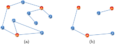
  Figure 2: Illustration of graph of strong dependence (GOSD). Red: signal nodes. Blue: noise nodes. (a) GOSD with 10 nodes. (b) Nodes of GOSD that survived the $\mathit{PS}$-step.

  where $W$ is a random vector and $Q$ can be thought of as the covariance matrix of $W$. Define $W_{\hat{N}}$, a subvector of $W$, and $Q_{\hat{N},\hat{N}}$, a submatrix of $Q$, as follows:

  $$W_{\hat{N}} = \bigl{(}B^{{\mathcal{I}}^{ps},\hat{N}}\bigr{)}^{\prime}\bigl{(}H^{{\mathcal{I}}^{ps},{\mathcal{I}}^{ps}}\bigr{)}^{-1}d^{{\mathcal{I}}^{ps}},$$

  $$Q_{\hat{N},\hat{N}} = \bigl{(}B^{{\mathcal{I}}^{ps},\hat{N}}\bigr{)}^{\prime}\bigl{(}H^{{\mathcal{I}}^{ps},{\mathcal{I}}^{ps}}\bigr{)}^{-1}\bigl{(}B^{{\mathcal{I}}^{ps},\hat{N}}\bigr{)}.$$

  Introduce the test statistic

  $$T(d,\hat{F},\hat{N})=W^{\prime}Q^{-1}W-W_{\hat{N}}^{\prime}(Q_{\hat{N},\hat{N}})^{-1}W_{\hat{N}}.$$ (20)

  For a threshold $t=t(\hat{F},\hat{N})$ to be determined, we update the set of retained nodes by ${\mathcal{U}}^{(t)}={\mathcal{U}}^{(t-1)}\cup\hat{F}$ if $T(d,\hat{F},\hat{N})>t$, and let ${\mathcal{U}}^{(t)}={\mathcal{U}}^{(t-1)}$ otherwise. In other words, we accept nodes in $\hat{F}$ only when they have additional utilities.

The $\mathit{PS}$-step terminates at $t=T$. We then write ${\mathcal{U}}_{p}^{*}={\mathcal{U}}^{(T)}$ so that

$${\mathcal{U}}_{p}^{*}=\mbox{the set of all retained indices at the end of the $\mathit{PS}$-step}.$$

In the $\mathit{PS}$-step, as we screen, we accept nodes sequentially. Once a node is accepted in the $\mathit{PS}$-step, it stays there until the end of the $\mathit{PS}$-step; of course, this node could be killed in the $\mathit{PE}$-step. In spirit, this is similar to the well-known forward regression method, but the implementation of two methods are significantly different.

The $\mathit{PS}$-step uses a collection of tuning thresholds

$${\mathcal{Q}}=\bigl{\{}t(\hat{F},\hat{N})\dvtx\mbox{$(\hat{F},\hat{N})$ are defined above}\bigr{\}}.$$

A convenient choice for these thresholds is to let $t(\hat{F},\hat{N})=2\tilde{q}\log(p)|\hat{F}|$ for a properly small fixed constant $\tilde{q}>0$. See Section 2.9 (and also Sections 2.10–2.11) for more discussion on the choices of $t(\hat{F},\hat{N})$.

In the $\mathit{PS}$-step, we use $\chi^{2}$-test for screening. This is the best choice when the coordinates of $z$ are Gaussian and have the same variance. When the Gaussian assumption on $z$ is questionable, we must note that the $\chi^{2}$-test depends on the Gaussianity of $a^{\prime}z$ for all $p$-different $a$, not on that of $z$; $a^{\prime}z$ could be approximately Gaussian by central limit theorem. Therefore, the performance of $\chi^{2}$-test is relatively robust to non-Gaussianity. If circumstances arise that the $\chi^{2}$-test is not appropriate (e.g., misspecification of the model, low quantity of the data), we may need an alternative, say, some nonparametric tests. In this case, if the efficiency of the test is nearly optimal, then the screening in the $\mathit{PS}$-step would continue to be successful.

How does the $\mathit{PS}$-step help in variable selection? In Section A in Ke, Jin and Fan (2014), we show that in a broad context, provided that the tuning parameters $t(\hat{F},\hat{N})$ are properly set, the $\mathit{PS}$-step has two noteworthy properties: the sure screening (SS) property and the separable after screening (SAS) property. The SS property says that ${\mathcal{U}}_{p}^{*}$ contains all but a negligible fraction of the true signals. The SAS property says that if we view ${\mathcal{U}}_{p}^{*}$ as a subgraph of ${\mathcal{G}}^{*}$ (more precisely, as a subgraph of ${\mathcal{G}}^{+}$, an expanded graph of ${\mathcal{G}}^{*}$ to be introduce below), then this subgraph decomposes into many disconnected components, each having a moderate size.

Together, the SS property and the SAS property enable us to reduce the original large-scale problem to many parallel small-size regression problems, and pave the way for the $\mathit{PE}$-step. See Section A in Ke, Jin and Fan (2014) for details.

Example 2(b).

We illustrate the above points with the toy example in Example 2(a). Suppose after the $\mathit{PS}$-step, the set of retained indices ${\mathcal{U}}_{p}^{*}$ is $\{1,4,5,7,8,9\}$; see Figure 2(b). In this example, we have a total of three signal nodes, $\{1\}$, $\{4\}$ and $\{8\}$, which are all retained in ${\mathcal{U}}_{p}^{*}$ and so the $\mathit{PS}$-step yields sure screening. On the other hand, ${\mathcal{U}}_{p}^{*}$ contains a few nodes of false positives, which will be further cleaned in the $\mathit{PE}$-step. At the same time, viewing it as a subgraph of ${\mathcal{G}}^{*}$, ${\mathcal{U}}_{p}^{*}$ decomposes into two disconnected components, $\{1,7,8,9\}$ and $\{4,5\}$; compare Figure 2(a). The SS property and the SAS property enable us to reduce the original problem of $10$ nodes to two parallel regression problems, one with $4$ nodes, and the other with $2$ nodes.

We now discuss the $\mathit{PE}$-step. Recall that $\ell^{pe}$ is the tuning parameter for the patching of the $\mathit{PE}$-step, and let $\{i\}^{pe}$ be as in Definition 2.6. The following graph can be viewed as an expanded graph of ${\mathcal{G}}^{*}$.

Definition 2.7.

Let ${\mathcal{G}}^{+}=(V,E)$ be the graph where $V=\{1,2,\ldots,p\}$ and there is an edge between nodes $i$ and $j$ when there exist nodes $k\in\{i\}^{pe}$ and $k^{\prime}\in\{j\}^{pe}$ such that there is an edge between $k$ and $k^{\prime}$ in ${\mathcal{G}}^{*}$.

Recall that ${\mathcal{U}}_{p}^{*}$ is the set of retained indices at the end of the $\mathit{PS}$-step.

Definition 2.8.

Fix a graph ${\mathcal{G}}$ and its subgraph ${\mathcal{I}}$. We say ${\mathcal{I}}\unlhd{\mathcal{G}}$ if ${\mathcal{I}}$ is a connected subgraph of ${\mathcal{G}}$, and ${\mathcal{I}}\lhd{\mathcal{G}}$ if ${\mathcal{I}}$ is a component (maximal connected subgraph) of ${\mathcal{G}}$.

Fix $1\leq j\leq p$. When $j\notin{\mathcal{U}}_{p}^{*}$, CASE estimates $\beta_{j}$ as $0$. When $j\in{\mathcal{U}}_{p}^{*}$, viewing ${\mathcal{U}}_{p}^{*}$ as a subgraph of ${\mathcal{G}}^{+}$, there is a unique subgraph ${\mathcal{I}}$ such that $j\in{\mathcal{I}}\lhd{\mathcal{U}}_{p}^{*}$. Fix two tuning parameters $u^{pe}$ and $v^{pe}$. We estimate $\beta^{{\mathcal{I}}}$ by minimizing

$$\min_{\theta}\biggl{\{}\frac{1}{2}\bigl{(}d^{{\mathcal{I}}^{pe}}-B^{{\mathcal{I}}^{pe},{\mathcal{I}}}\theta\bigr{)}^{\prime}\bigl{(}H^{{\mathcal{I}}^{pe},{\mathcal{I}}^{pe}}\bigr{)}^{-1}\bigl{(}d^{{\mathcal{I}}^{pe}}-B^{{\mathcal{I}}^{pe},{\mathcal{I}}}\theta\bigr{)}$$

(21)

$$\hskip 180.0pt{}+\frac{(u^{pe})^{2}}{2}\|\theta\|_{0}\biggr{\}},$$

subject to that $\theta$ is an $|{\mathcal{I}}|\times 1$ vector each of which nonzero coordinate $\geq v^{pe}$, where $\|\theta\|_{0}$ denotes the $L^{0}$-norm of $\theta$. Putting these together gives the final estimator of CASE $\hat{\beta}^{\mathrm{case}}=\hat{\beta}^{\mathrm{case}}(Y;\delta,m,{\mathcal{Q}},\ell^{ps},\ell^{pe},u^{pe},v^{pe},D_{h,\eta},X,p)$.

CASE uses tuning parameters ($\delta,m,{\mathcal{Q}},\ell^{ps},\ell^{pe},u^{pe},v^{pe}$). Earlier in this paper, we have briefly discussed how to choose $(\delta,{\mathcal{Q}})$. As for $m$, usually, a choice of $m=2$ or $3$ is sufficient unless the signals are relatively “dense.” The choices of $(\ell^{ps},\ell^{pe},u^{pe},v^{pe})$ are addressed in Section 2.9; see also Sections 2.10–2.11.

2.6 Computational complexity of CASE, comparison with multivariate screening

The $\mathit{PS}$-step is closely related to the well-known method of marginal screening and has a moderate computational complexity.

Marginal screening selects variables by thresholding the vector $d$ coordinate-wise. The method is computationally fast, but it neglects “local” graphical structures, and is thus ineffective. For this reason, in many challenging problems, it is desirable to use multivariate screening methods which adapt to “local” graphical structures.

Fix $m>1$. An $m$-variate $\chi^{2}$-screening procedure is one of such desired methods. The method screens all $k$-tuples of coordinates of $d$ using $\chi^{2}$-tests, for all $k\leq m$, in an exhaustive (brute-force) fashion. Seemingly, the method adapts to “local” graphical structures and could be much more effective than marginal screening. However, such a procedure has a computational cost of $O(p^{m})$ [excluding the computational cost for obtaining $X^{\prime}Y$ from $(X,Y)$; same below] which is usually not affordable when $p$ is large.

The main innovation of the $\mathit{PS}$-step is to use a graph-assisted $m$-variate $\chi^{2}$-screening, which is both effective in variable selection and efficient in computation. In fact, the $\mathit{PS}$-step only screens $k$-tuples of coordinates of $d$ that form a connected subgraph of ${\mathcal{G}}^{*}$, for all $k\leq m$. Therefore, if ${\mathcal{G}}^{*}$ is $K$-sparse, then there are $\leq Cp(eK)^{m+1}$ connected subgraphs of ${\mathcal{G}}^{*}$ with size $\leq m$; so if $K=K_{p}$ is no greater than a multi-$\log(p)$ term (see Definition 2.10), then the computational complexity of the $\mathit{PS}$-step is only $O(p)$, up to a multi-$\log(p)$ term.

Example 2(c).

We illustrate the difference between the above three methods with the toy example in Example 2(a), where $p=10$ and the GOSD is displayed in Figure 2(a). Suppose we choose $m=3$. Marginal screening screens all $10$ single nodes of the GOSD. The brute-force $m$-variate screening screens all $k$-tuples of indices, $1\leq k\leq m$, with a total of ${p\choose 1}+\cdots+{p\choose m}=175$ such $k$-tuples. The $m$-variate screening in the $\mathit{PS}$-step only screens $k$-tuples that are connected subgraphs of ${\mathcal{G}}^{*}$, for $1\leq k\leq m$, and in this example, we only have $30$ such connected subgraphs.

The computational complexity of the $\mathit{PE}$-step consists two parts. The first part is the complexity of obtaining all components of ${\mathcal{U}}_{p}^{*}$, which is $O(pK)$ and where $K$ is the maximum degree of ${\mathcal{G}}^{+}$; note that for settings considered in this paper, $K=K_{p}^{+}$ does not exceed a multi-$\log(p)$ term [see Lemma B.2 in Ke, Jin and Fan (2014)]. The second part of the complexity comes from solving (2.5), which hinges on the maximal size of ${\mathcal{I}}$. In Lemma A.2 in Ke, Jin and Fan (2014), we show that in a broad context, the maximal size of ${\mathcal{I}}$ does not exceed a constant $l_{0}$, provided the thresholds ${\mathcal{Q}}$ are properly set. Numerical studies in Section 3 also support this point. Therefore, the complexity in this part does not exceed $p\cdot 3^{l_{0}}$. As a result, the computational complexity of the $\mathit{PE}$-step is moderate. Here, the bound $O(pK+p\cdot 3^{l_{0}})$ is conservative; the actual computational complexity is much smaller than this.

How does CASE perform? In Sections 2.7–2.9, we set up an asymptotic framework and show that CASE is asymptotically minimax in terms of the Hamming distance over a wide class of situations. In Sections 2.10–2.11, we apply CASE to the long-memory time series and the change-point model, and elaborate the optimality of CASE in such models with the so-called phase diagram.

2.7 Asymptotic rare and weak model

In this section, we add an asymptotic framework to the rare and weak signal model $RW(\varepsilon,\tau,\mu)$ introduced in Section 2.1. We use $p$ as the driving asymptotic parameter and tie $(\varepsilon,\tau)$ to $p$ through some fixed parameters.

In particular, we fix $\vartheta\in(0,1)$ and model the sparse parameter $\varepsilon$ by

$$\varepsilon=\varepsilon_{p}=p^{-\vartheta}.$$ (22)

Note that as $p$ grows, the signal becomes increasingly sparse. It turns out that the most interesting range of signal strength is $\tau=O(\sqrt{\log(p)})$; see, for example, Ji and Jin (2012). For much smaller $\tau$, successful recovery is impossible. For much larger $\tau$, the problem is relatively easy. The critical value of $\tau$ depends on $\vartheta$ in a complicate way. In light of this, we fix $r>0$, and let

$$\tau=\tau_{p}=\sqrt{2r\log(p)}.$$ (23)

At the same time, recalling that in $RW(\varepsilon,\tau,\mu)$, we require $\mu\in\Theta_{p}(\tau)$ so that $|\mu_{i}|\geq\tau$ for all $1\leq i\leq p$. Fixing $a>1$, we now further restrict $\mu$ to the following subset of $\Theta_{p}(\tau)$:

$$\Theta_{p}^{*}(\tau_{p},a)=\bigl{\{}\mu\in\Theta_{p}(\tau_{p})\dvtx\tau_{p}\leq|\mu_{i}|\leq a\tau_{p},1\leq i\leq p\bigr{\}}.$$ (24)

Definition 2.9.

We call (22)–(24) the asymptotic rare and weak model $\mathit{ARW}(\vartheta,r,a,\mu)$.

Requiring the strength of each signal $\leq a\tau_{p}$ is mainly for technical reasons, and hopefully, such a constraint can be removed in the near future. From a practical point of view, since usually we do not have sufficient information on $\mu$, we prefer to have a larger $a$: we hope that when $a$ is properly large, $\Theta_{p}^{*}(\tau_{p},a)$ is broad enough, so that neither the optimal procedure nor the minimax risk needs to adapt to $a$.

Toward this end, we impose some mild regularity conditions on $a$ and the Gram matrix $G$. Let $g$ be the smallest integer such that

$$g\geq\max\bigl{\{}(\vartheta+r)^{2}/(2\vartheta r),m\bigr{\}}.$$ (25)

For any $p\times p$ Gram matrix $G$ and $1\leq k\leq p$, let $\lambda_{k}^{*}(G)$ be the minimum of the smallest eigenvalues of all $k\times k$ principle sub-matrices of $G$. Introduce

$$\widetilde{{\mathcal{M}}}_{p}(c_{0},g)=\bigl{\{}\mbox{$G$ is a $p\times p$ Gram matrix, $\lambda_{k}^{*}(G)\geq c_{0}$, $1\leq k\leq g$}\bigr{\}}.$$ (26)

For any two subsets $V_{0}$ and $V_{1}$ of $\{1,2,\ldots,p\}$, consider the optimization problem

$$\bigl{(}\theta^{(0)}_{*}(V_{0},V_{1};G),\theta_{*}^{(1)}(V_{0},V_{1};G)\bigr{)}$$

$$\qquad=\operatorname{argmin}\bigl{\{}\bigl{(}\theta^{(1)}-\theta^{(0)}\bigr{)}^{\prime}G\bigl{(}\theta^{(1)}-\theta^{(0)}\bigr{)}\bigr{\}},$$

up to the constraints that $|\theta_{i}^{(k)}|\geq\tau_{p}$ if $i\in V_{k}$ and $\theta_{i}^{(k)}=0$ otherwise, where $k=0,1$, and that in the special case of $V_{0}=V_{1}$, the sign vectors of $\theta^{(0)}$ and $\theta^{(1)}$ are unequal. Introduce

$$a_{g}^{*}(G)=\max_{\{(V_{0},V_{1})\dvtx|V_{0}\cup V_{1}|\leq g\}}\max\bigl{\{}\bigl{\|}\theta_{*}^{(0)}(V_{0},V_{1};G)\bigr{\|}_{\infty},\bigl{\|}\theta_{*}^{(1)}(V_{0},V_{1};G)\bigr{\|}_{\infty}\bigr{\}}.$$

The following lemma is elementary, so we omit the proof.

Lemma 2.3

For any $G\in\widetilde{{\mathcal{M}}}_{p}(c_{0},g)$, there is a constant $C=C(c_{0},g)>0$ such that $a_{g}^{*}(G)\leq C$.

In this paper, except for Section 2.11 where we discuss the change-point model, we assume

$$G\in\widetilde{{\mathcal{M}}}(c_{0},g),\qquad a>a^{*}_{g}(G).$$ (27)

Under such conditions, $\Theta_{p}^{*}(\tau_{p},a)$ is broad enough and the minimax risk (to be introduced below) does not depend on $a$. See Section 2.8 for more discussion.

For any variable selection procedure $\hat{\beta}$, we measure the performance by the Hamming distance

$$h_{p}(\hat{\beta};\beta,G)=E\Biggl{[}\sum_{j=1}^{p}1\bigl{\{}\operatorname{sgn}(\hat{\beta}_{j})\neq\operatorname{sgn}(\beta_{j})\bigr{\}}\Big{|}X,\beta\Biggr{]},$$

where the expectation is taken with respect to $\hat{\beta}$. Here, for any $p\times 1$ vector $\xi$, $\operatorname{sgn}(\xi)$ denotes the sign vector [for any number $x$, $\operatorname{sgn}(x)=1,0,-1$ when $x<0$, $x=0$, and $x>0$ correspondingly].

Under $\mathit{ARW}(\vartheta,r,a,\mu)$, $\beta=b\circ\mu$, so the overall Hamming distance is

$$H_{p}(\hat{\beta};\varepsilon_{p},\mu,G)=E_{\varepsilon_{p}}\bigl{[}h_{p}(\hat{\beta};\beta,G)|X\bigr{]},$$

where $E_{\varepsilon_{p}}$ is the expectation with respect to the law of $b$. Finally, the minimax Hamming distance under $\mathit{ARW}(\vartheta,r,a,\mu)$ is

$$\operatorname{Hamm}_{p}^{*}(\vartheta,r,a,G)=\inf_{\hat{\beta}}\sup_{\mu\in\Theta_{p}^{*}(\tau_{p},a)}H_{p}(\hat{\beta};\varepsilon_{p},\mu,G).$$

In next section, we will see that the minimax Hamming distance does not depend on $a$ as long as (27) holds.

In many recent works, the probability of exact support recovery or oracle property is used to assess optimality; see, for example, Fan and Li (2001), Zhao and Yu (2006), Fan, Xue and Zou (2014), Zou (2006). However, when signals are rare and weak, exact support recovery is usually impossible, and the Hamming distance is a more appropriate criterion for assessing optimality. In comparison, study on the minimax Hamming distance is not only mathematically more demanding but also scientifically more relevant than that on the oracle property.

2.8 Lower bound for the minimax Hamming distance

We view the(global) Hamming distance as the aggregation of “local” Hamming errors. To construct a lower bound for the (global) minimax Hamming distance, the key is to construct lower bounds for “local” Hamming errors. Fix $1\leq j\leq p$. The “local” Hamming error at index $j$ is the risk we make among the neighboring indices of $j$ in GOSD, say, $\{k\dvtx d(j,k)\leq g\}$, where $g$ is as in (25) and $d(j,k)$ is the geodesic distance between $j$ and $k$ in the GOSD. The lower bound for such a “local” Hamming error is characterized by an exponent $\rho_{j}^{*}$, which we now introduce.

For any subset $V\subset\{1,2,\ldots,p\}$, let $I_{V}$ be the $p\times 1$ vector such that the $j$th coordinate is $1$ if $j\in V$ and $0$ otherwise. Fixing two subsets $V_{0}$ and $V_{1}$ of $\{1,2,\ldots,p\}$, we introduce

$$\varpi^{*}(V_{0},V_{1})=\tau_{p}^{-2}\min_{\theta^{(0)},\theta^{(1)}}\bigl{\{}\bigl{(}\theta^{(1)}-\theta^{(0)}\bigr{)}^{\prime}G\bigl{(}\theta^{(1)}-\theta^{(0)}\bigr{)}\bigr{\}},$$ (28)

subject to $\{\theta^{(k)}=I_{V_{k}}\circ\mu^{(k)}\dvtx\mu^{(k)}\in\Theta_{p}^{*}(\tau_{p},a),k=0,1,\operatorname{sgn}(\theta^{(0)})\neq\operatorname{sgn}(\theta^{(1)})\}$, and let

$$\rho(V_{0},V_{1}) = \max\bigl{\{}|V_{0}|,|V_{1}|\bigr{\}}\vartheta$$

$${}+\frac{1}{4}\biggl{[}\biggl{(}\sqrt{\varpi^{*}(V_{0},V_{1})r}-\frac{|(|V_{1}|-|V_{0}|)|\vartheta}{\sqrt{\varpi^{*}(V_{0},V_{1})r}}\biggr{)}_{+}\biggr{]}^{2}.$$

The exponent $\rho_{j}^{*}=\rho_{j}^{*}(\vartheta,r,a,G)$ is defined by

$$\rho_{j}^{*}(\vartheta,r,a,G)=\min_{(V_{0},V_{1})\dvtx j\in V_{0}\cup V_{1}}\rho(V_{0},V_{1}).$$ (30)

The notation $L_{p}$ is frequently used in this paper.

Definition 2.10.

$L_{p}$, as a positive sequence indexed by $p$, is called a multi-$\log(p)$ term if for any fixed $\delta>0$, $\lim_{p\rightarrow\infty}L_{p}p^{\delta}=\infty$ and$\lim_{p\rightarrow\infty}L_{p}p^{-\delta}=0$.

It can be shown that $L_{p}p^{-\rho_{j}^{*}}$ provides a lower bound for the “local” minimax Hamming distance at index $j$, and that when (27) holds, $\rho_{j}^{*}(\vartheta,r,a,G)$ does not depend on $a$; see Lemma 16 in Jin, Zhang and Zhang (2014) for details. In the remaining part of the paper, we will write it as $\rho_{j}^{*}(\vartheta,r,G)$ for short.

At the same time, in order for the aggregation of all lower bounds for “local” Hamming errors to give a lower bound for the “global” Hamming distance, we need to introduce graph of least favorables (GOLF). Toward this end, recalling $g$ and $\rho(V_{0},V_{1})$ as in (25) and (2.8), respectively, let

$$\bigl{(}V_{0j}^{*},V_{1j}^{*}\bigr{)}=\mathop{\operatorname{argmin}\limits_{\{(V_{0},V_{1})\dvtx j\in V_{0}\cup V_{1},|V_{0}\cup V_{1}|\leq g\}}}\rho(V_{0},V_{1}),$$

and when there is a tie, pick the one that appears first lexicographically. We can think $(V_{0j}^{*},V_{1j}^{*})$ as the “least favorable” configuration at index $j$.

Definition 2.11.

GOLF is the graph ${\mathcal{G}}^{\diamond}=(V,E)$ where $V=\{1,2,\ldots,p\}$ and there is an edge between $j$ and $k$ if and only if $(V_{0j}^{*}\cup V_{1j}^{*})\cap(V_{0k}^{*}\cup V_{1k}^{*})\neq\varnothing$.

The following theorem is similar to Theorem 14 in Jin, Zhang and Zhang (2014), so we omit the proof.

Theorem 2.1

Suppose (27) holds so that $\rho_{j}^{*}(\vartheta,r,a,G)$ does not depend on the parameter $a$ for sufficiently large $p$. As $p\to\infty$, $\operatorname{Hamm}^{*}_{p}(\vartheta,r,a,\break G)\geq L_{p}[d_{p}({\mathcal{G}}^{\diamond})]^{-1}\sum_{j=1}^{p}p^{-\rho_{j}^{*}(\vartheta,r,G)}$, where $d_{p}({\mathcal{G}}^{\diamond})$ is the maximum degree of all nodes in ${\mathcal{G}}^{\diamond}$.

In many examples, including those of primary interest of this paper,

$$d_{p}\bigl{(}{\mathcal{G}}^{\diamond}\bigr{)}\leq L_{p}.$$ (31)

In such cases, we have the following lower bound:

$$\operatorname{Hamm}^{*}_{p}(\vartheta,r,a,G)\geq L_{p}\sum_{j=1}^{p}p^{-\rho_{j}^{*}(\vartheta,r,G)}.$$ (32)

2.9 Upper bound and optimality of CASE

In this section, we show that in a broad context, provided the tuning parameters are properly set, CASE achieves the lower bound prescribed in Theorem 2.1, up to some $L_{p}$ terms. Therefore, the lower bound in Theorem 2.1 is tight, and CASE achieves the optimal rate of convergence.

For a given $\gamma>0$, we focus on linear models with the Gram matrix from

$${\mathcal{M}}_{p}^{*}(\gamma,g,c_{0},A_{1})=\widetilde{{\mathcal{M}}}_{p}(c_{0},g)\cap\mathcal{M}_{p}(\gamma,A_{1}),$$

where we recall that the two terms on the right-hand side are defined in (2.2) and (26), respectively. The following lemma is proved in Section B in Ke, Jin and Fan (2014).

Lemma 2.4

For $G\in\mathcal{M}^{*}_{p}(\gamma,g,c_{0},A_{1})$, the maximum degree of nodes in GOLF satisfies $d_{p}({\mathcal{G}}^{\diamond})\leq L_{p}$.

Combining Lemma 2.4 with Theorem 2.1, the lower bound (32) holds.

For any linear filter $D=D_{h,\eta}$, let $\varphi_{\eta}(z)=1+\eta_{1}z+\cdots+\eta_{h}z^{h}$ be the so-called characterization polynomial. We need some regularity conditions:

• Regularization Condition A (RCA). For any root $z_{0}$ of $\varphi_{\eta}(z)$, $|z_{0}|\geq 1$.

• Regularization Condition B (RCB). There are constants $\kappa>0$ and $c_{1}>0$ such that $\lambda_{k}^{*}(DGD^{\prime})\geq c_{1}k^{-\kappa}$ ($\lambda_{k}^{*}$ is as in Section 2.8).

For many well-known linear filters such as adjacent differences, seasonal differences, etc., RCA is satisfied. Also, RCB is only a mild condition since $\kappa$ can be any positive number. For example, RCB holds in the change-point model and long-memory time series model with certain $D$ matrices. In general, $\kappa$ is not $0$ because when $DG$ is sparse, $DGD^{\prime}$ is very likely to be approximately singular, and the associated value of $\lambda_{k}^{*}$ can be small when $k$ is large. This is true even for very simple $G$ [e.g., $G=I_{p}$, $D=D_{1,\eta}$ and $\eta=(1,-1)^{\prime}$].

At the same time, these conditions can be further relaxed. For example, for the change-point problem, the Gram matrix has barely any off-diagonal decay, and does not belong to ${\mathcal{M}}_{p}^{*}$. Nevertheless, with slight modification in the procedure, the main results continue to hold.

CASE uses tuning parameters $(\delta,m,{\mathcal{Q}},\ell^{ps},\ell^{pe},u^{pe},v^{pe})$. The choice of $\delta$ is flexible, and we usually set $\delta=1/\log(p)$. For the main theorem below, we treat $m$ as given. In practice, taking $m$ to be a small integer (say, $\leq 3$) is usually sufficient, unless the signals are relatively dense (say, $\vartheta<1/4$). The choice of $\ell^{ps}$ and $\ell^{pe}$ are also relatively flexible, and letting $\ell^{ps}$ be a sufficiently large constant and $\ell^{pe}$ be $(\log(p))^{\nu}$ for some constant $\nu<(1-1/\alpha)/(\kappa+1/2)$ is sufficient, where $\alpha$ is as in Definition 2.2, and $\kappa$ is as in RCB.

At the same time, in principle, the optimal choices of $(u^{pe},v^{pe})$ are

$$u^{pe}=\sqrt{2\vartheta\log p},\qquad v^{pe}=\sqrt{2r\log p},$$ (33)

which depend on the underlying parameters $(\vartheta,r)$ that are unknown to us. Despite this, our numeric studies in Section 3 suggest that the choices of $(u^{pe},v^{pe})$ are relatively flexible; see Sections 3–4 for more discussions.

Last, we discuss how to choose ${\mathcal{Q}}=\{t(\hat{F},\hat{N})\dvtx\mbox{$(\hat{F},\hat{N})$ are defined as in the}$ $\mbox{$\mathit{PS}$-step}\}$. Let $t(\hat{F},\hat{N})=2q\log(p)$, where $q>0$ is a constant. It turns out that the main result (Theorem 2.2 below) holds as long as

$$q_{0}\leq q\leq q^{*}(\hat{F},\hat{N}),$$ (34)

where $q_{0}>0$ is an appropriately small constant, and for any subsets $(F,N)$,

$$q^{*}(F,N)$$

$$\qquad=\max\bigl{\{}q\dvtx\bigl{(}|F|+|N|\bigr{)}\vartheta+\bigl{[}\bigl{(}\sqrt{\tilde{\omega}(F,N)r}-\sqrt{q|F|}\bigr{)}_{+}\bigr{]}^{2}\geq\psi(F,N)\bigr{\}};$$

here,

$$\quad\psi(F,N) = \frac{(|F|+2|N|)\vartheta}{2}$$

$${}+\cases{\displaystyle\frac{1}{4}\omega(F,N)r,\qquad|F|\mbox{ is even},\vspace*{2pt}\cr\displaystyle\frac{\vartheta}{2}+\frac{1}{4}\bigl{[}\bigl{(}\sqrt{\omega(F,N)r}-\vartheta/\sqrt{\omega(F,N)r}\bigr{)}_{+}\bigr{]}^{2},\vspace*{2pt}\cr\hskip 78.0pt|F|\mbox{ is odd},}$$

with

$$\omega(F,N)=\min_{\xi\in\mathbb{R}^{|F|}\dvtx|\xi_{i}|\geq 1}\xi^{\prime}\bigl{[}G^{F,F}-G^{F,N}\bigl{(}G^{N,N}\bigr{)}^{-1}G^{N,F}\bigr{]}\xi$$ (37)

and

$$\tilde{\omega}(F,N)=\min_{\xi\in\mathbb{R}^{|F|}\dvtx|\xi_{i}|\geq 1}\xi^{\prime}\bigl{[}Q_{F,F}-Q_{F,N}(Q_{N,N})^{-1}Q_{N,F}\bigr{]}\xi,$$ (38)

where $Q_{F,N}=(B^{{\mathcal{I}}^{ps},F})^{\prime}(H^{{\mathcal{I}}^{ps},{\mathcal{I}}^{ps}})^{-1}(B^{{\mathcal{I}}^{ps},N})$ with ${\mathcal{I}}=F\cup N$, and $Q_{N,F}$, $Q_{F,F}$ and $Q_{N,N}$ are defined similarly. Compared to (• ‣ 2.5), we see that $Q_{F,N}$, $Q_{F,N}$, $Q_{N,F}$ and $Q_{N,N}$ are all submatrices of $Q$. Hence, $\tilde{\omega}(F,N)$ can be viewed as a counterpart of $\omega(F,N)$ by replacing the submatrices of $G^{{\mathcal{I}},{\mathcal{I}}}$ by the corresponding ones of $Q$.

From a practical point of view, there is a trade-off in choosing $q$: a larger $q$ would increase the number of falsely selected variables in the $\mathit{PS}$-step, but would also reduce the computational cost in the $\mathit{PE}$-step. The following is a convenient choice which we recommend in this paper:

$$t(\hat{F},\hat{N})=2\tilde{q}|\hat{F}|\log(p),$$ (39)

where $0<\tilde{q}<c_{0}r/4$ is a constant, and $c_{0}$ is as in ${\mathcal{M}}_{p}^{*}(\gamma,g,c_{0},A_{1})$.

We are now ready for the main result of this paper.

Theorem 2.2

Suppose that for sufficiently large $p$, $G\in{\mathcal{M}}_{p}^{*}(\gamma,g,c_{0},A_{1})$, $D_{h,\eta}G\in\mathcal{M}_{p}(\alpha,A_{0})$ with $\alpha>1$ and that RCA-RCB hold. Consider $\hat{\beta}^{\mathrm{case}}=\hat{\beta}^{\mathrm{case}}(Y;\delta,m,{\mathcal{Q}},\ell^{ps},\ell^{pe},u^{pe},v^{pe},D_{h,\eta},X,p)$ with the tuning parameters specified above. Then as $p\rightarrow\infty$,

$$\sup_{\mu\in\Theta_{p}^{*}(\tau_{p},a)}H_{p}\bigl{(}\hat{\beta}^{\mathrm{case}};\varepsilon_{p},\mu,G\bigr{)}$$

(40)

$$\qquad\leq L_{p}\Biggl{[}p^{1-(m+1)\vartheta}+\sum_{j=1}^{p}p^{-\rho_{j}^{*}(\vartheta,r,G)}\Biggr{]}+o(1).$$

Combine Lemma 2.4 and Theorem 2.2. Given the parameter $m$ is appropriately large, both the upper bound and the lower bound are tight, and CASE achieves the optimal rate of convergence prescribed by

$$\operatorname{Hamm}_{p}^{*}(\vartheta,r,a,G)=L_{p}\sum_{j=1}^{p}p^{-\rho_{j}^{*}(\vartheta,r,G)}+o(1).$$ (41)

Theorem 2.2 is proved in Section A in Ke, Jin and Fan (2014), where we explain the key idea behind the procedure, as well as the selection of the tuning parameters.

2.10 Application to the long-memory time series model

The long-memory time series model in Section 1 can be written as a regression model,

$$Y=X\beta+z,\qquad z\sim N(0,I_{n}),$$

where the Gram matrix $G$ is asymptotically Toeplitz and has slow off-diagonal decays. Without loss of generality, we consider the following idealized case where $G$ is an exact Toeplitz matrix generated by a spectral density $f$:

$$G(i,j)=\frac{1}{2\pi}\int_{-\pi}^{\pi}\cos\bigl{(}|i-j|\omega\bigr{)}f(\omega)\,d\omega,\qquad 1\leq i,j\leq p.$$ (42)

In the literature [Chen, Hurvich and Lu (2006), Moulines and Soulier (1999)], the spectral density for a long-memory process is usually characterized as

$$f(\omega)=\bigl{|}1-e^{\sqrt{-1}\omega}\bigr{|}^{-2\phi}f^{*}(\omega),$$ (43)

where $\phi\in(0,1/2)$ is the long-memory parameter, $f^{*}(\omega)$ is a positive symmetric function that is continuous on $[-\pi,\pi]$ and is twice differentiable except at $\omega=0$.

In this model, the Gram matrix is nonsparse, but it is sparsifiable. To see the point, let $\eta=(1,-1)^{\prime}$ and let $D=D_{1,\eta}$ be the first-order adjacent row-differencing. On one hand, since the spectral density $f$ is singular at the origin, it follows from the Fourier analysis that $|G(i,j)|\geq C(1+|i-j|)^{-(1-2\phi)}$, and hence $G$ is nonsparse. On the other hand, it is seen that

$$B(i,j)=\sqrt{-1}\int_{|j-i|}^{|j-i|+1}\widehat{\omega f(\omega)}(\lambda)\,d\lambda,$$

where we recall that $B=DG$ and note that $\hat{g}$ denotes the Fourier transform of $g$. Compared to $f(\omega)$, $\omega f(\omega)$ is nonsingular at the origin. Additionally, it is seen that $B\in\mathcal{M}_{p}(2-2\phi,A)$, where $2-2\phi>1$, so $B$ is sparse (a similar claim applies to $H=DGD^{\prime}$). This shows that $G$ is sparsifiable by adjacent row-differencing.

In this example, there is a function $\rho_{\mathrm{lts}}^{*}(\vartheta,r;f)$ that only depends on $(\vartheta,r,f)$ such that

$$\max_{\{j\dvtx\log(p)\leq j\leq p-\log(p)\}}\bigl{\{}\bigl{|}\rho_{j}^{*}(\vartheta,r,G)-\rho_{\mathrm{lts}}^{*}(\vartheta,r;f)\bigr{|}\bigr{\}}\rightarrow 0\qquad\mbox{as $p\rightarrow\infty$},$$

where the subscript “lts” stands for long-memory time series. The following theorem can be derived from Theorem 2.2, and is proved in Section B in Ke, Jin and Fan (2014).

Theorem 2.3

For a long-memory time series model where $|(f^{*})^{\prime\prime}(\omega)|\leq C|\omega|^{-2}$, the minimax Hamming distance then satisfies $\operatorname{Hamm}_{p}^{*}(\vartheta,r,G)=L_{p}p^{1-\rho_{\mathrm{lts}}^{*}(\vartheta,r;f)}$. If we apply CASE by letting $(m+1)\vartheta>\rho_{\mathrm{lts}}^{*}(\vartheta,r;f)$, $\eta=(1,-1)^{\prime}$, and the tuning parameters be set as in Section 2.9, then

$$\sup_{\mu\in\Theta_{p}^{*}(\tau_{p},a)}H_{p}\bigl{(}\hat{\beta}^{\mathrm{case}};\varepsilon_{p},\mu,G\bigr{)}\leq L_{p}p^{1-\rho_{\mathrm{lts}}^{*}(\vartheta,r;f)}+o(1).$$

Theorem 2.3 can be interpreted by the so-called phase diagram. Phase diagram is a way to visualize settings where the signals are so rare and weak that successful variable selection is simply impossible [Ji and Jin (2012)]. In detail, for a spectral density $f$ and $\vartheta\in(0,1)$, let $r_{\mathrm{lts}}^{*}(\vartheta)=r_{\mathrm{lts}}^{*}(\vartheta;f)$ be the unique solution of $\rho_{\mathrm{lts}}^{*}(\vartheta,r;f)=1$. Note that $r=r^{*}_{\mathrm{lts}}(\vartheta)$ characterizes the minimum signal strength required for exact support recovery with high probability. The following proposition is proved in Section B in Ke, Jin and Fan (2014).

Lemma 2.5

Under the conditions of Theorem 2.3, if $(f^{*})^{\prime\prime}(0)$ exists, then $r^{*}_{\mathrm{lts}}(\vartheta;f)$ is a decreasing function in $\vartheta$, with limits $1$ and $\frac{2}{\pi}\int_{-\pi}^{\pi}f^{-1}(\omega)\,d\omega$ as $\vartheta\rightarrow 1$ and $\vartheta\rightarrow 0$, respectively.

Call the two-dimensional space $\{(\vartheta,r)\dvtx 0<\vartheta<1,r>0\}$ the phase space. Interestingly, there is a partition of the phase space as follows.

• Region of no recovery $\{(\vartheta,r)\dvtx 0<r<\vartheta,0<\vartheta<1\}$. In this region, the minimax Hamming distance $\gtrsim p\varepsilon_{p}$, where $p\varepsilon_{p}$ is approximately the number of signals. In this region, the signals are too rare and weak and successful variable selection is impossible.

• Region of almost full recovery $\{(\vartheta,r):\vartheta<r<r_{\mathrm{lts}}^{*}(\vartheta;f),0<\vartheta<1\}$. In this region, the minimax Hamming distance is much larger than $1$ but much smaller than $p\varepsilon_{p}$. Therefore, the optimal procedure can recover most of the signals but not all of them.

• Region of exact recovery $\{(\vartheta,r):r>r_{\mathrm{lts}}^{*}(\vartheta;f),0<\vartheta<1\}$. In this region, the minimax Hamming distance is $o(1)$. Therefore, the optimal procedure recovers all signals with probability $\approx 1$.

Because of the partition of the phase space, we call this the phase diagram.

From time to time, we wish to have a more explicit formula for the rate $\rho_{\mathrm{lts}}^{*}(\vartheta,r;f)$ and the critical value $r_{\mathrm{lts}}^{*}(\vartheta;f)$. In general, this is a hard problem, but both quantities can be computed numerically when $f$ is given. In Figure 3, we display the phase diagrams for the autoregressive fractionally integrated moving average process (FARIMA) with parameters $(0,\phi,0)$ [Fan and Yao (2003)], where

$$f^{*}(\omega)=\frac{\Gamma^{2}(1-\phi)}{\Gamma(1-2\phi)}.$$ (44)

Take $\phi=0.35,0.25$, for example, $r_{\mathrm{lts}}^{*}(\vartheta;f)\approx 7.14,5.08$ for small $\vartheta$.

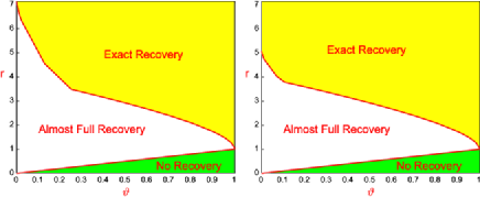
Figure 3: Phase diagrams corresponding to the $\operatorname{FARIMA}(0,\phi,0)$ process. Left: $\phi=0.35$. Right: $\phi=0.25$.

2.11 Application to the change-point model

The change-point model in the Introduction can be viewed as a special case of model (1), where $\beta$ is as in (7), and the Gram matrix satisfies

$$G(i,j)=\min\{i,j\},\qquad 1\leq i,j\leq p.$$ (45)

For technical reasons, it is more convenient not to normalize the diagonals of $G$ to $1$.

The change-point model can be viewed as an “extreme” case of what is studied in this paper. On one hand, the Gram matrix $G$ is “ill-posed,” and each row of $G$ does not satisfy the condition of off-diagonal decay in Theorem 2.2. On the other hand, $G$ has a very special structure which can be largely exploited. In fact, if we sparsify $G$ using the linear filter $D=D_{2,\eta}$, where $\eta=(1,-2,1)^{\prime}$, it is seen that $B=DG=I_{p}$, and $H=DGD^{\prime}$ is a tri-diagonal matrix with $H(i,j)=2\cdot 1\{i=j\}-1\{|i-j|=1\}-1\{i=j=p\}$, which are very simple matrices. For these reasons, we modify the CASE as follows:

• Due to the simple structure of $B$, we do not need patching in the $\mathit{PS}$-step (i.e., $\ell^{ps}=0$).

• For the same reason, the choices of thresholds $t(\hat{F},\hat{N})$ are more flexible than before, and taking $t(\hat{F},\hat{N})=2q\log(p)$ for a proper constant $q>0$ works.

• Since $H$ is “extreme” (the smallest eigenvalue tends to $0$ as $p\rightarrow\infty$), we have to modify the $\mathit{PE}$-step carefully.

In detail, the $\mathit{PE}$-step for the change-point model is as follows. Given $\ell^{pe}$, let ${\mathcal{G}}^{+}$ be as in Definition 2.7. Recall that ${\mathcal{U}}_{p}^{*}$ denotes the set of all retained indices at the end of the $\mathit{PS}$-step. We view ${\mathcal{U}}_{p}^{*}$ as a subgraph of ${\mathcal{G}}^{+}$, and let ${\mathcal{I}}\lhd{\mathcal{U}}_{p}^{*}$ be one of its components. The goal is to split ${\mathcal{I}}$ into $N$ different subsets

$${\mathcal{I}}={\mathcal{I}}^{(1)}\cup\cdots\cup{\mathcal{I}}^{(N)},$$

and for each subset ${\mathcal{I}}^{(k)}$, $1\leq k\leq N$, we construct a patched set ${\mathcal{I}}^{(k),pe}$. We then estimate $\beta^{{\mathcal{I}}^{(k)}}$ separately using (2.5). Putting $\beta^{{\mathcal{I}}^{(k)}}$ together gives our estimate of $\beta^{{\mathcal{I}}}$.

The subsets $\{({\mathcal{I}}^{(k)},{\mathcal{I}}^{(k),pe})\}_{k=1}^{N}$ are recursively constructed as follows. Denote $l=|{\mathcal{I}}|$, $M=(\ell^{pe}/2)^{1/(l+1)}$, and write

$${\mathcal{I}}=\{j_{1},j_{2},\ldots,j_{l}\},\qquad j_{1}<j_{2}<\cdots<j_{l}.$$

First, letting $k_{1}$ be the largest index such that $j_{k_{1}}-j_{k_{1}-1}>\ell^{pe}/M$, define

$${\mathcal{I}}^{(1)}=\{j_{k_{1}},\ldots,j_{l}\}\quad\mbox{and}\quad{\mathcal{I}}^{(1),pe}=\bigl{\{}j_{k_{1}}-\ell^{pe}/(2M),\ldots,j_{l}+\ell^{pe}/2\bigr{\}}.$$

Next, letting $k_{2}<k_{1}$ be the largest index such that $j_{k_{2}}-j_{k_{2}-1}>\ell^{pe}/M^{2}$, define

$${\mathcal{I}}^{(2)}=\{j_{k_{2}},\ldots,j_{k_{1}}\},\qquad{\mathcal{I}}^{(2),pe}=\bigl{\{}j_{k_{2}}-\ell^{pe}/\bigl{(}2M^{2}\bigr{)},\ldots,j_{k_{1}}+\ell^{pe}/(2M)\bigr{\}}.$$

Continue this process until for some $N$, $1\leq N\leq l$, $k_{N}=1$. In this construction, for each $1\leq k\leq N$, if we arrange all the nodes of ${\mathcal{I}}^{(k),pe}$ in the ascending order, then the number of nodes in front of ${\mathcal{I}}^{(k)}$ is significantly smaller than the number of nodes behind ${\mathcal{I}}^{(k)}$.

In practice, we introduce a suboptimal but much simpler patching approach as follows. Fix a component ${\mathcal{I}}=\{j_{1},\ldots,j_{l}\}$ of ${\mathcal{U}}_{p}^{*}$. In this approach, instead of splitting it into smaller sets and patching them separately as in the previous approach, we patch the whole set ${\mathcal{I}}$ by

$${\mathcal{I}}^{pe}=\bigl{\{}i\dvtx j_{1}-\ell^{pe}/4<i<j_{l}+3\ell^{pe}/4\bigr{\}},$$ (46)

and estimate $\beta^{{\mathcal{I}}}$ using (2.5). Our numeric studies show that two approaches have comparable performances.

Define

$$\rho^{*}_{\mathrm{cp}}(\vartheta,r)=\cases{\vartheta+r/4,&\quad$r/\vartheta\leq 6+2\sqrt{10},$\vspace*{2pt}\cr 3\vartheta+(r/2-\vartheta)^{2}/(2r),&\quad$r/\vartheta>6+2\sqrt{10},$}$$ (47)

where “cp” stands for change-point. Choose the tuning parameters of CASE such that

$$\quad\ell^{pe}=2\log(p),\qquad u^{pe}=\sqrt{2\vartheta\log(p)}\quad\mbox{and}\quad v^{pe}=\sqrt{2r\log(p)},$$ (48)

that $(m+1)\vartheta\geq\rho^{*}_{\mathrm{cp}}(\vartheta,r)$, and that $0<q<\frac{r}{4}(\sqrt{2}-1)^{2}$ [recall that we take $t(\hat{F},\hat{N})=2q\log(p)$ for all $(\hat{F},\hat{N})$ in the change-point setting]. Note that the choice of $\ell^{pe}$ is different from that in Section 2.5. The main result in this section is the following theorem which is proved in Section B in Ke, Jin and Fan (2014).

Theorem 2.4

For the change-point model, the minimax Hamming distance satisfies $\operatorname{Hamm}_{p}^{*}(\vartheta,r,G)=L_{p}p^{1-\rho^{*}_{\mathrm{cp}}(\vartheta,r)}$. Furthermore, $\hat{\beta}^{\mathrm{case}}$ with the tuning parameters specified above satisfies

$$\sup_{\mu\in\Theta_{p}^{*}(\tau_{p},a)}H_{p}\bigl{(}\hat{\beta}^{\mathrm{case}};\varepsilon_{p},\mu,G\bigr{)}\leq L_{p}p^{1-\rho^{*}_{\mathrm{cp}}(\vartheta,r)}+o(1).$$

It is noteworthy that the exponent $\rho_{\mathrm{cp}}^{*}(\vartheta,r)$ has a phase change depending on the ratios of $r/\vartheta$. The insight is, when $r/\vartheta<6+2\sqrt{10}$, the minimax Hamming distance is dominated by the Hamming errors we make in distinguishing between an isolated change-point and a pair of adjacent change-points, and when $r/\vartheta>6+2\sqrt{10}$, the minimax Hamming distance is dominated by the Hamming errors of distinguishing the case of consecutive change-point triplets (say, change-points at $\{j-1,j,j-1\}$) from the case where we do not have a change-point in the middle of the triplets (i.e., the change-points are only at $\{j-1,j+1\}$).

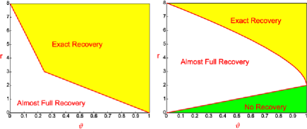
Figure 4: Phase diagrams corresponding to the change-point model. Left: CASE; the boundary is decided by $(4-10\vartheta)+2\sqrt{(2-5\vartheta)^{2}-\vartheta^{2}}$ (left part) and $4(1-\vartheta)$ (right part). Right: hard thresholding; the upper boundary is decided by $2(1+\sqrt{1-\vartheta})^{2}$ and the lower boundary is decided by $2\vartheta$.

Similarly, the main results on the change-point problem can be visualized with the phase diagram in Figure 4. An interesting point is that it is possible to have almost full recovery even when the signal strength parameter $\tau_{p}$ is as small as $o(\sqrt{2\log(p)})$. See the proof of Theorem 2.4 for details.

Alternatively, one may apply the following approach to the change-point problem. Treat the liner change-point model as a regression model $Y=X\beta+z$ as in Section 1 (page 1), and let $W=(X^{\prime}X)^{-1}X^{\prime}Y$ be the least-squares estimate. It is seen that $W\sim N(\beta,\Sigma)$, where we note that $\Sigma=(X^{\prime}X)^{-1}$ is tridiagonal and coincides with $H$. In this simple setting, a natural approach is to apply a coordinate-wise thresholding $\hat{\beta}^{\mathrm{thresh}}_{j}=W_{j}1\{|W_{j}|>t\}$ to locate the signals. But this neglects the covariance of $W$ in detecting the locations of the signals and is not optimal even with the ideal choice of thresholding parameter $t_{0}$, since the corresponding risk satisfies

$$\sup_{\{\mu\in\Theta_{p}^{*}(\tau_{p},a)\}}H_{p}\bigl{(}\hat{\beta}^{\mathrm{thresh}}(t_{0});\varepsilon_{p},\mu,G\bigr{)}=L_{p}p^{1-(r/2+\vartheta)^{2}/(2r)}.$$

The proof of this is elementary and omitted. The phase diagram of this method is displayed in Figure 4, right panel, which suggests the method is nonoptimal.

Other popular methods in locating multiple change-points include the global methods [Harchaoui and Lévy-Leduc (2010), Olshen et al. (2004), Tibshirani (1996), Yao and Au (1989)] and local methods [e.g., SaRa in Niu and Zhang (2012)]. The global methods are usually computationally expensive and can hardly be optimal due to the strong correlation nature of this problem. Our procedure is related to the local methods but is different in important ways. Our method exploits the graphical structures and uses the GOSD to guide both the screening and cleaning, but SaRa does not utilize the graphical structures and can be shown to be nonoptimal.

To conclude the section, we remark that the change-point model constitutes a special case of the settings we discuss in the paper, where setting some of the tuning parameters is more convenient than in the general case. First, for the change-point model, we can simply set $\delta=0$ and $\ell^{ps}=0$. Second, there is an easy-to-compute preliminary estimator available. On the other hand, the performance of CASE is substantially better than the other methods in many situations. We believe that CASE is potentially a very useful method in practice for the change-point problem.

3 Simulations

We conducted a small-scale numeric study where we compare CASE and several popular approaches. The study contains two parts, Section 3.1 and Section 3.2, where we investigate the change-point model and the long-memory time series model, respectively.

In this section, $s_{p}=p\varepsilon_{p}$ for convenience. The core tuning parameters for CASE are $({\mathcal{Q}},u^{pe},v^{pe},\ell^{ps},\ell^{pe})$. We streamline these tuning parameters in a way so they only depend on two tuning parameters $(s_{p},\tau_{p})$ (calibrating the sparsity and the minimum signal strength, resp.). Therefore, essentially, CASE only uses two tuning parameters. Our experiments show that the performance of CASE is relatively insensitive to these two tuning parameters. Furthermore, these two tuning parameters can be set in a data driven fashion, especially in the change-point model. See details below.

We set $m=2$ so that in the screening stage of CASE, bivariate screening is the highest order screening we use. At least for examples considered here, using a higher-order screening does not have a significant improvement. For long-memory time series, we need a regularization parameter $\delta$ (but we do not need it for the change-point model). The guideline for choosing $\delta$ is to make sure the maximum degree of GOSD is $15$ (say) or smaller. In this section, we choose $\delta=2.5/\log(p)$. The maximum degree of GOSD is much higher if we choose a much smaller $\delta$; in this case, CASE has similar performance, but is computationally much slower.

3.1 Change-point model

In this section, we use model (3) to investigate the performance of CASE in identifying multiple change-points. For a given set of parameters $(p,\vartheta,r,a)$, we set $\varepsilon_{p}=p^{-\vartheta}$ and $\tau_{p}=\sqrt{2r\log(p)}$. First, we generate a $(p-1)\times 1$ vector $\beta$ by $\beta_{j}\stackrel{{\scriptstyle\mathrm{i.i.d.}}}{{\sim}}(1-\varepsilon_{p})\nu_{0}+\frac{\varepsilon_{p}}{2}U(\tau_{p},a\tau_{p})+\frac{\varepsilon_{p}}{2}U(-a\tau_{p},-\tau_{p})$, where $U(s,t)$ is the uniform distribution over $[s,t]$ [when $s=t$, $U(s,t)$ represents the point mass at $s$]. Next, we construct the mean vector $\theta$ in model (3) by $\theta_{j}=\theta_{j-1}+\beta_{j-1}$, $2\leq j\leq p$. Last, we generate the data vector $Y$ by $Y\sim N(\theta,I_{p})$.

CASE, when applied to the change-point model, requires tuning parameters $(m,\delta,{\mathcal{Q}},\ell^{ps},\ell^{pe},u^{pe},v^{pe})$. Denote by $s_{p}\equiv p\varepsilon_{p}=p^{1-\vartheta}$ the average number of signals. Given $(s_{p},\tau_{p})$, we determine the tuning parameters as follows: As mentioned earlier, we take $m=2$, $\delta=0$ and $\ell^{ps}=0$. Also, we take $\ell^{pe}=10\log(p/s_{p})$, $u^{pe}=\sqrt{2\log(p/s_{p})}$ and $v^{pe}=\tau_{p}$. ${\mathcal{Q}}$ contains thresholds $t(F,N)$ for each pair of sets $(F,N)$; we take $t(F,N)=2q(F,N)\log(p)$ with

$$q(F,N)=0.8\times\cases{\bigl{(}r\tilde{\omega}+|F|\vartheta\bigr{)}^{2}/(4r\tilde{\omega}),&\quad$\tilde{\omega}>|F|\vartheta,$\vspace*{2pt}\cr r\tilde{\omega},&\quad$\tilde{\omega}\leq|F|\vartheta,$}$$ (49)

where $\vartheta=\log(p/s_{p})$, $r=\tau_{p}^{2}/(2\log(p))$ and $\tilde{\omega}=\tilde{\omega}(F,N)$ is given in (38). With these choices, CASE only depends on two parameters $(s_{p},\tau_{p})$.

Experiment 1a. We compare CASE with the lasso [Tibshirani (1996)], SCAD [Fan and Li (2001)] (penalty shape parameter $a=3.7$), MC$+$ [Zhang (2010)] (penalty shape parameter $\gamma=1.1$) and SaRa [Niu and Zhang (2012)]. For tuning parameters $\lambda>0$ and $h>0$ (integer), SaRa takes the following form:

$$\hat{\beta}_{i}^{\mathrm{SaRa}}=W_{i}\cdot 1\bigl{\{}|W_{i}|>\lambda\bigr{\}}\qquad\mbox{where }W_{i}=\frac{1}{h}\Biggl{(}\sum_{j=i+1}^{i+h}Y_{j}-\sum_{j=i-h+1}^{i}Y_{j}\Biggr{)}.$$

The tuning parameters for the lasso, SCAD, MC$+$ and SaRa are ideally set (pretending we know $\beta$). For CASE, all tuning parameters depend on $(s_{p},\tau_{p})$, so we implement the procedure using the true values of $(s_{p},\tau_{p})$; this yields slightly inferior results than that of setting $(s_{p},\tau_{p})$ ideally (pretending we know $\beta$, as we do in the lasso, SCAD, MC$+$ and SaRa), so our comparison in this setting is fair. Note that even when $(s_{p},\tau_{p})$ are given, it is unclear how to set the tuning parameters of the lasso, SCAD, MC$+$ and SaRa.

Fix $p=5000$ and $a=1$. We let $\vartheta$ range in $\{0.3,0.45,0.6,0.75\}$ and $\tau_{p}$ range in $\{3,3.5,\ldots,6.5\}$. The parameters fall into the regime where exact-recovery is impossible. Table 1 reports the average Hamming errors of $100$ independent repetitions. We see that CASE consistently outperforms other methods, especially when $\vartheta$ is small, that is, signals are less sparse.

We also observe that three global penalization methods, the lasso, SCAD and MC$+$, perform unsatisfactorily, with Hamming errors comparable to the expected number of signals $s_{p}$. It suggests that the global penalization methods are not appropriate for the change-point model when the signals are rare and weak. Similar conclusions can be drawn in most experiments in this section. To save space, we only report results of the lasso, SCAD and MC$+$ in this experiment.

Table 1: Comparison of Hamming errors (Experiment 1a; change-point model)

$\bolds{\vartheta}$	$\bolds{s_{p}}$		$\bolds{\tau_{p}}$
			$4.0$	$4.5$	$5.0$	$5.5$	$6.0$	$6.5$
0.3	$338.4$	CASE	$105.8$	$63.9$	$37.6$	$18.5$	$8.9$	$4.8$
		lasso	$371.7$	$370.0$	$371.5$	$370.1$	$371.5$	$369.8$
		SCAD	$370.6$	$368.3$	$370.5$	$368.2$	$369.3$	$369.2$
		MC$+$	$374.0$	$372.1$	$374.3$	$372.5$	$373.6$	$373.1$
		SaRa	$175.6$	$144.0$	$107.8$	$73.7$	$49.0$	$32.3$
			$3.0$	$3.5$	$4.0$	$4.5$	$5.0$	$5.5$
0.45	$108.3$	CASE	$50.1$	$35.5$	$26.3$	$20.0$	$12.8$	$6.2$
		lasso	$103.2$	$104.1$	$103.8$	$103.8$	$104.9$	$104.3$
		SCAD	$101.8$	$102.7$	$102.1$	$102.0$	$102.9$	$102.5$
		MC$+$	$103.7$	$104.7$	$104.4$	$104.3$	$105.4$	$104.8$
		SaRa	$78.9$	$72.0$	$66.2$	$63.4$	$61.9$	$60.4$
			$3.0$	$3.5$	$4.0$	$4.5$	$5.0$	$5.5$
0.6	$30.2$	CASE	$14.4$	$11.1$	$8.9$	$6.7$	$5.0$	$3.9$
		lasso	$29.3$	$29.2$	$29.3$	$29.7$	$27.7$	$29.3$
		SCAD	$27.7$	$27.7$	$27.9$	$27.4$	$26.1$	$27.1$
		MC$+$	$29.8$	$29.8$	$29.8$	$30.2$	$28.4$	$29.8$
		SaRa	$20.4$	$17.0$	$13.6$	$10.9$	$8.6$	$6.8$
			$3.0$	$3.5$	$4.0$	$4.5$	$5.0$	$5.5$
0.75	$8.4$	CASE	$3.5$	$2.9$	$2.4$	$1.8$	$1.6$	$1.3$
		lasso	$8.2$	$8.3$	$8.5$	$8.8$	$8.0$	$8.5$
		SCAD	$6.8$	$7.0$	$7.0$	$6.9$	$6.6$	$6.6$
		MC$+$	$8.7$	$8.8$	$9.1$	$9.2$	$8.7$	$9.1$
		SaRa	$5.2$	$4.5$	$3.8$	$3.0$	$2.4$	$2.0$

Experiment 1b. In this experiment, we investigate the performanceof CASE with $(s_{p},\tau_{p})$ estimated by SaRa; we call this the adaptiveCASE. In detail, we estimate $(s_{p},\tau_{p})$ by $\hat{s}_{p}=\sum_{j=1}^{p}1\{\hat{\beta}^{\mathrm{SaRa}}_{j}\neq 0\}$ and $\hat{\tau}_{p}=\break\operatorname{median}(\{|\hat{\beta}^{\mathrm{SaRa}}_{j}|:\hat{\beta}_{j}^{\mathrm{SaRa}}\neq 0\})$, where the tuning parameters $(\lambda,h)$ of SaRa are determined by minimizing $\operatorname{BIC}(\hat{\beta})=\frac{1}{2}\|Y-X\hat{\beta}\|^{2}+\log(p)\cdot\|\hat{\beta}\|_{0}$; this is a slight modification of Bayesian information criteria (BIC).

For experiment, we use the same setting as in Experiment 1a. Table 2 reports the average Hamming errors of CASE, SaRa and the adaptive CASE based on $100$ independent repetitions. First, the adaptive CASE [CASE but $(s_{p},\tau_{p})$ are estimated by SaRa] has a very similar performance to CASE. Second, although the adaptive CASE uses SaRa as the preliminary estimator, its performance is substantially better than that of SaRa (and other methods in the same setting; see Experiment 1a).

Table 2: Comparison of Hamming errors (Experiment 1b). “adCASE” stands for adaptive CASE, where $(s_{p},\tau_{p})$ are estimated from SaRa [where $(\lambda,h)$ are set by BIC]

$\bolds{\vartheta}$	$\bolds{s_{p}}$		$\bolds{\tau_{p}}$
			$4.0$	$4.5$	$5.0$	$5.5$	$6.0$	$6.5$
0.3	$338.4$	CASE	$105.8$	$63.9$	$37.6$	$18.5$	$8.9$	$4.8$
		adCASE	$100.3$	$63.6$	$37.8$	$18.6$	$8.9$	$4.8$
		SaRa	$190.7$	$162.0$	$131.3$	$98.0$	$68.2$	$47.1$
			$3.0$	$3.5$	$4.0$	$4.5$	$5.0$	$5.5$
0.45	$108.3$	CASE	$50.1$	$35.5$	$26.3$	$20.0$	$12.8$	$6.2$
		adCASE	$48.6$	$33.9$	$26.0$	$20.8$	$16.6$	$9.7$
		SaRa	$86.1$	$76.7$	$71.4$	$66.7$	$65.0$	$62.8$
			$3.0$	$3.5$	$4.0$	$4.5$	$5.0$	$5.5$
0.6	$30.2$	CASE	$14.4$	$11.1$	$8.9$	$6.7$	$5.0$	$3.9$
		adCASE	$14.0$	$11.0$	$8.8$	$6.5$	$4.8$	$3.4$
		SaRa	$35.7$	$28.5$	$24.1$	$19.9$	$15.8$	$11.9$
			$3.0$	$3.5$	$4.0$	$4.5$	$5.0$	$5.5$
0.75	$8.4$	CASE	$3.5$	$2.9$	$2.4$	$1.8$	$1.6$	$1.3$
		adCASE	$3.7$	$3.0$	$2.2$	$1.8$	$1.5$	$1.3$
		SaRa	$13.3$	$11.5$	$8.0$	$5.2$	$4.0$	$2.9$

Experiment 2. In this experiment, we consider the post-filtering model, model (4), associated with the change-point model, and illustrate that the seeming simplicity of this model (where $DG=I_{p}$, and $DGD^{\prime}$ is tri-diagonal) does not mean it is a trivial setting for variable selection. In particular, if we naively apply the $L^{0}/L^{1}$-penalization to the post-filtering model, we end up with naive soft/hard thresholding; we illustrate our point by showing that CASE significantly outperforms naive thresholding (since we use Hamming distance as the loss function, there is no difference between soft and hard thresholding). For both CASE and naive thresholding, we set tuning parameters assuming $(s_{p},\tau_{p})$ as known. The threshold of naive thresholding is set as $(r+2\vartheta)^{2}/(2r)\cdot\log(p)$, where $\vartheta=\log(p/s_{p})$ and $r=\tau_{p}^{2}/(2\log(p))$; this threshold choice is known as theoretically optimal.

Fix $p=10^{6}$ and $a=1$ (so that the signals have equal strengths). Let $\vartheta$ range in $\{0.35,0.5,0.75\}$, and $\tau_{p}$ range in $\{5,\ldots,13\}$. Table 3 reports the average Hamming errors of $50$ independent repetitions, which show that CASE outperforms naive thresholding in most cases, especially when $\vartheta$ is small or $\tau_{p}$ is small. It suggests that the post-filtering model remains largely nontrivial, and to deal with it, we need sophisticated methods.

Table 3: Comparison of Hamming errors (Experiment 2; change-point model), $p=10^{6}$. “nHT” stands for naive hard thresholding

			$\bolds{\tau_{p}}$
$\bolds{\vartheta}$	$\bolds{s_{p}}$		5	6	7	8	9	10	11	12	13
0.35	$7943$	CASE	$956.7$	$332.6$	$117.5$	$49.1$	$24.1$	$13.9$	$10.6$	$7.7$	7.3
		nHT	$4430.5$	$2381.3$	$1085.8$	$418.1$	$139.7$	$41.9$	$11.0$	$2.5$	0.5
0.50	$1000$	CASE	$195.3$	$68.8$	$20.8$	$5.0$	$1.3$	$0.7$	$0.4$	$0.1$	0.2
		nHT	$767.9$	$489.0$	$250.8$	$105.3$	$38.4$	$12.4$	$3.5$	$0.7$	0.2
0.75	$32$	CASE	$9.3$	$3.1$	$2.3$	$0.4$	$0.1$	$0.1$	$0.1$	$0.0$	0.0
		nHT	$31.1$	$25.6$	$15.7$	$8.3$	$3.2$	$1.8$	$0.5$	$0.0$	0.0

Experiment 3. In this experiment, we fix $(p,\vartheta,\tau_{p})=(5000,0.50,4.5)$, and let $a$ range in $\{1,1.5,\ldots,3\}$ (so signals may have different strengths). We investigate a case where the signals have the “half-positive-half-negative” sign pattern, that is, $\beta_{j}\stackrel{{\scriptstyle\mathrm{i.i.d.}}}{{\sim}}(1-\varepsilon_{p})\nu_{0}+\frac{\varepsilon_{p}}{2}U(\tau_{p},a\tau_{p})+\frac{\varepsilon_{p}}{2}U(-a\tau_{p},-\tau_{p})$, and a case where the signals have the “all-positive” sign pattern, that is, $\beta_{j}\stackrel{{\scriptstyle\mathrm{i.i.d.}}}{{\sim}}(1-\varepsilon_{p})\nu_{0}+\varepsilon_{p}U(\tau_{p},a\tau_{p})$. We compare CASE with SaRa for different values of $a$ and sign patterns (we do not include the lasso, SCAD, MC$+$ in this particular experiment, for at least for the experiments reported above, they are inferior to SaRa). The tuning parameters for both CASE and SaRa are set ideally as in Experiment 1a. The results of $50$ independent repetitions are reported in Table 4, which suggest that CASE uniformly outperforms SaRa for various values of $a$ and the two sign patterns.

Table 4: Comparison of Hamming errors (Experiment 3; change-point model) for different choices of $a$ (the ratio between the maximum and minimum signal strengths) and for two sign patterns “half–half” and “all positive.” $p=5000$, $\vartheta=0.5$, $s_{p}=70.7$ and $\tau_{p}=4.5$

		$\bolds{a}$
		1	1.5	2	2.5	3
Half–half	CASE	$14.26$	$6.32$	$5.50$	$4.78$	$4.56$
	SaRa	$24.98$	$18.96$	$16.56$	$14.00$	$12.50$
All-positive	CASE	$13.44$	$6.18$	$4.90$	$5.38$	$4.14$
	SaRa	$24.26$	$18.58$	$16.80$	$13.66$	$12.12$

3.2 Long-memory time series model

In this section, we investigate long-memory time series, focusing on the $\operatorname{FARIMA}(0,\phi,0)$ process [Fan and Yao (2003)], where $\phi$ is the long-memory parameter. We let $X=G^{1/2}$ where $G$ is constructed according to (42)–(44). For $\beta$ generated in ways to be specified, we let $Y\sim N(X\beta,I_{p})$.

CASE uses tuning parameters $(m,\delta,{\mathcal{Q}},\ell^{ps},\ell^{pe},u^{pe},v^{pe})$, which are set in the same way as in the change-point model, except for two differences. First, different from that in the change-point model, we need a regularization parameter $\delta$ which we set as $2.5/\log(p)$. Second, we take $\ell^{ps}=\ell^{pe}/2$.

Experiment 4a. In this experiment, we compare CASE with the lasso, SCAD (shape parameter $a=3.7$) and MC$+$ (shape parameter $\gamma=2$). Fixing $p=5000$ and $\phi=0.35$, we let $\vartheta$ range in $\{0.35,0.45,0.55\}$, and let $\tau_{p}$ range in $\{4,\ldots,8\}$. For each pair of $(\vartheta,\tau_{p})$, we generate the vector $\beta$ by $\beta_{j}\stackrel{{\scriptstyle\mathrm{i.i.d.}}}{{\sim}}(1-\varepsilon_{p})\nu_{0}+\frac{\varepsilon_{p}}{2}\nu_{\tau_{p}}+\frac{\varepsilon_{p}}{2}\nu_{-\tau_{p}}$. Similar to that in Experiment 1a, the tuning parameters of CASE are set assuming $(s_{p},\tau_{p})$ as known, and the tuning parameters of the lasso, SCAD and MC$+$ are set ideally to minimize the Hamming error (assuming $\beta$ is known). By similar argument as in Experiment 1a, the comparison is fair. Table 5 reports the average Hamming errors based on $100$ independent repetitions. The results suggest that CASE outperforms the lasso and SCAD, and has a comparable performance to that of MC$+$.

Table 5: Comparison of Hamming errors (Experiment 4a). The Gram matrix is the population covariance matrix of the $\operatorname{FARIMA}(0,\phi,0)$ process with $\phi=0.35$. $p=5000$

			$\bolds{\tau_{p}}$
$\bolds{\vartheta}$	$\bolds{s_{p}}$		4	5	6	7	8
0.35	$253.7$	CASE	$118.0$	$60.7$	$26.3$	$9.5$	$4.3$
		lasso	$145.2$	$91.6$	$60.2$	$37.4$	$26.0$
		SCAD	$140.6$	$87.0$	$42.8$	$19.5$	$8.0$
		MC$+$	$108.6$	$50.2$	$20.4$	$7.4$	$2.6$
0.45	$108.3$	CASE	$60.3$	$27.7$	$11.8$	$4.0$	$1.9$
		lasso	$65.6$	$40.0$	$23.2$	$13.5$	$7.7$
		SCAD	$64.0$	$37.7$	$19.6$	$9.2$	$3.9$
		MC$+$	$52.0$	$23.6$	$8.6$	$3.0$	$1.0$
0.55	$46.2$	CASE	$27.9$	$13.4$	$4.3$	$1.4$	$0.5$
		lasso	$27.8$	$16.0$	$8.0$	$3.9$	$2.1$
		SCAD	$27.0$	$15.2$	$7.0$	$3.1$	$1.2$
		MC$+$	$23.4$	$10.6$	$3.1$	$0.7$	$0.2$

Experiment 4b. We investigate the setting where “signal cancellation” is more severe than that in Experiment 4b. Toward this end, we use the same setting as in Experiment 4a, except for that $\beta$ is generated in a way that signals appear in adjacent pairs with opposite signs, $(\beta_{2j-1},\beta_{2j})\stackrel{{\scriptstyle\mathrm{i.i.d.}}}{{\sim}}(1-\varepsilon_{p})\nu_{(0,0)}+\varepsilon_{p}\nu_{(\tau_{p},-\tau_{p})}$, $1\leq j\leq p/2$, where $\nu_{(a,b)}$ is the point mass at $(a,b)\in\mathbb{R}^{2}$. Hamming errors based on $100$ repetitions are reported in Table 6, suggesting that CASE significantly outperforms all the other methods.

It is noteworthy that MC$+$ behaves much more unsatisfactorily here than in Experiment 4a, and the main reason is that MC$+$ does not adequately address “signal cancellation.” In contrast, one of the major advantages of CASE is that it addresses adequately the “signal cancellation”; this is why it has satisfactory performance in both Experiments 4a and 4b.

Table 6: Comparison of Hamming errors (Experiment 4b)

			$\bolds{\tau_{p}}$
$\bolds{\vartheta}$	$\bolds{s_{p}}$		4	5	6	7	8
0.35	$253.7$	CASE	$138.6$	$60.8$	$23.3$	$7.2$	$1.8$
		lasso	$223.0$	$158.9$	$97.9$	$54.8$	$27.1$
		SCAD	$257.5$	$156.8$	$95.1$	$52.1$	$25.1$
		MC$+$	$206.7$	$129.2$	$68.6$	$33.4$	$13.6$
0.45	$108.3$	CASE	$75.7$	$36.4$	$13.3$	$3.7$	$0.9$
		lasso	$100.0$	$84.7$	$58.4$	$32.2$	$15.9$
		SCAD	$99.2$	$83.2$	$56.6$	$30.6$	$14.9$
		MC$+$	$98.1$	$76.0$	$44.8$	$21.5$	$8.9$
0.55	$46.2$	CASE	$38.6$	$20.0$	$8.9$	$3.6$	$1.0$
		lasso	$45.4$	$40.1$	$31.0$	$20.6$	$10.9$
		SCAD	$45.0$	$39.4$	$30.1$	$19.6$	$9.9$
		MC$+$	$44.9$	$38.4$	$26.3$	$14.8$	$6.8$

Table 7: Hamming errors for CASE, applied when $(s_{p},\tau_{p})$ are misspecified as $p^{1-\tilde{\vartheta}}$ and $\tilde{\tau}_{p}$, respectively (Experiment 5). The Gram matrix is the population covariance matrix of the $\operatorname{FARIMA}(0,\phi,0)$ process with $\phi=0.35$. $p=5000$

$\vartheta=0.35,\tau_{p}=6$	$\tilde{\vartheta}$	$0.2$	$0.25$	$0.3$	$0.35$	$0.4$	$0.45$	$0.5$
$s_{p}=253.7$		$27.8$	$24.8$	$23.2$	$23.2$	$24.5$	$26.3$	$48.9$
	$\tilde{\tau}_{p}$	$4$	$5$	$5.5$	$6$	$6.5$	$7$	$8$
		$47.3$	$30.2$	$25.3$	$23.2$	$23.9$	$26.9$	$42.7$
$\vartheta=0.55,\tau_{p}=5$	$\tilde{\vartheta}$	$0.4$	$0.45$	$0.5$	$0.55$	$0.6$	$0.65$	$0.7$
$s_{p}=46.2$		$21.8$	$19.0$	$19.3$	$19.8$	$21.7$	$25.5$	$25.4$
	$\tilde{\tau}_{p}$	$3$	$4$	$4.5$	$5$	$5.5$	$6$	$7$
		$23.8$	$22.2$	$20.8$	$19.8$	$21.0$	$23.9$	$29.0$

Experiment 5. In some of the experiments above, we set the tuning parameters of CASE assuming $(s_{p},\tau_{p})$ as known. It is therefore interesting to investigate how the misspecification of $(s_{p},\tau_{p})$ affects the performance of CASE. Fix $p=5000$ and $\phi=0.35$. We consider two combinations of $(\vartheta,\tau_{p})$: $(\vartheta,\tau_{p})=(0.35,6),(0.55,5)$. The vector $\beta$ is generated in the same way as in Experiment 4b, with the signals appearing in adjacent pairs. We fix one parameter of $(s_{p},\tau_{p})$ and mis-specify the other [since $s_{p}$ is not on the same scale as $\tau_{p}$, the results are reported based on the misspecification of $(\vartheta,\tau_{p})$, instead of $(s_{p},\tau_{p})$; recall here $s_{p}=p^{1-\vartheta}$]. We then apply CASE with tuning parameters set based on the misspecified values of $(s_{p},\tau_{p})$. Table 7 reports the average Hamming errors of $50$ independent repetitions, which is a rather flat function of misspecified values of $\vartheta$ (with $\tau_{p}$ fixed) or of misspecified values of $\tau_{p}$ (with $\vartheta$ fixed). In comparison, the Hamming errors of the lasso are 97.9 and 40.1 in the two settings, respectively, with the tuning parameter ideally set as in Experiment 1a. This suggests that CASE is relatively insensitive to the misspecification of $(s_{p},\tau_{p})$, and outperforms the lasso as long as the misspecification of $(s_{p},\tau_{p})$ is not severe.

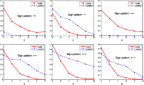
Figure 5: Comparison of Hamming errors (Experiment 6). The Gram matrix is the population covariance matrix of the $\operatorname{FARIMA}(0,\phi,0)$ process with $\phi=0.35$. $p=5000$, $\vartheta=0.75$ and $s_{p}=32$. Signals appear in adjacent pairs (Panels 1–2) or adjacent triplets (Panels 3–6), with different sign patterns specified in the panels, associated with different level of “signal cancellation.” CASE outperforms lasso when signal cancellation is severe.

Experiment 6. In this experiment, we continue to investigate the effect of “signal cancellation,” where we compare CASE with the lasso using several choices of signal patterns (and so the levels of “signal cancellation” vary). Fix $p=4998$, $\phi=0.35$, $\vartheta=0.75$, and let $\tau_{p}$ range in $\{5,\ldots,10\}$. The experiment contains two parts. In the first part, we partition $\{1,2,\ldots,p\}$ into $p/2$ blocks, where each block contains two adjacent indices. In $(1-\varepsilon_{p})$ fraction of the blocks, $\beta_{j}=0$. In the $\varepsilon_{p}$ fraction of the blocks, we have either that $\beta_{j}=\tau_{p}$ for both $j$ in the block (we denote the sign pattern by “$++$”), or that $\beta_{j}=\tau_{p}$ if $j$ is the first index in the block and $\beta_{j}=-\tau_{p}$ otherwise (sign pattern “$+-$”). In the second part, we partition $\{1,2,\ldots,p\}$ into $p/3$ blocks (block size is $3$), and generate $\beta$ in a similar fashion, but with four different sign patterns in each block: “$+++$,” “$++-$,” “$+-+$” and “$+--$.” Hamming errors based on $50$ independent repetitions are reported in Figure 5. The results suggest that (a) when the sign patterns are “$++$” or “$+++$,” signal cancellation has negligible effects, and CASE is inferior to the lasso, (b) when the sign patterns are “$+-$,” “$++-$,” “$+-+$” and “$+--$,” the effect of signal cancellation kicks in, and CASE outperforms the lasso in most cases. This is consistent with our theoretic insight that CASE adequately addresses signal cancellation, but the lasso does not.

4 Discussion

Variable selection when the Gram matrix $G$ is nonsparse is a challenging problem. We approach this problem by first sparsifying $G$ with a finite order linear filter, and then constructing a sparse graph GOSD. The key insight is that, in the post-filtering data, the true signals live in many small-size components that are disconnected in GOSD, but we do not know where. We propose CASE as a new approach to variable selection. This is a two-stage screen and clean method, where we first use a covariance-assisted multivariate screening to identify candidates for such small-size components, and then re-examine each candidate with penalized least squares. In both stages, to overcome the problem of information leakage, we employ a delicate patching technique.

We develop an asymptotic framework focusing on the regime where the signals are rare and weak so that successful variable selection is challenging but is still possible. We show that CASE achieves the optimal rate of convergence in Hamming distance across a wide class of situations where $G$ is nonsparse but sparsifiable. Such optimality cannot be achieved by many popular methods, including but not limited to the lasso, SCAD, MC$+$ and Dantzig selector. When $G$ is nonsparse, these methods are not expected to behave well even when the signals are strong. We have successfully applied CASE to two different applications: the change-point problem and the long-memory times series.

Compared to the well-known method of marginal screening [Fan and Song (2010), Wasserman and Roeder (2009)], CASE employs a covariance-assisted multivariate screening procedure, so that it is theoretically more effective than marginal screening, with only a moderate increase in the computational complexity. CASE is closely related to the graphical lasso [Friedman, Hastie and Tibshirani (2008), Meinshausen and Bühlmann (2006)], which also attempts to exploit the graph structure. However, the setting considered here is very different from that in Friedman, Hastie and Tibshirani (2008) and Meinshausen and Bühlmann (2006), and our emphasis on optimality is also very different.

The paper is closely related to the recent work Jin, Zhang and Zhang (2014) [see also Ji and Jin (2012)], but is different in important ways. The work in Jin, Zhang and Zhang (2014) is motivated by recent literature of compressive sensing and genetic regulatory network, and is largely focused on the case where the Gram matrix $G$ is sparse in an unstructured fashion. The current work is motivated by the recent interest on DNA-copy number variation and long-memory time series, and is focused on the case where there are strong dependence between different design variables, so $G$ is usually nonsparse and sometimes ill-posed. To deal with the strong dependence, we have to use a finite-order linear filter and delicate patching techniques. Additionally, the current paper also studies applications to the long-memory time series and the change-point problem which have not been considered in Jin, Zhang and Zhang (2014). Especially, the studies on the change-point problem encompasses very different and very delicate analysis on both the derivation of the lower bound and upper bound which we have not seen before in the literature. For these reasons, the two papers have very different scopes and techniques, and the results in one paper cannot be deduced from those in the other.

In this paper, we are primarily interested in the linear model, model (1), but CASE is applicable in much broader settings. For example, in model (1), we assume that the coordinates of $z$ have the same variance $\sigma^{2}$, and $\sigma$ is known (and so without loss of generality, we assume $\sigma=1$). When $\sigma$ is unknown, the main results in this paper continue to hold, provided that we can estimate $\sigma$ consistently [say, except for a probability of $o(p^{-2})$, there is an estimate $\hat{\sigma}$ such that $|\hat{\sigma}/\sigma-1|=o(1)$]. Such an estimator can be obtained by adapting the scaled-lasso approach by Sun and Zhang (2012) or the refitted cross validation by Fan, Guo and Hao (2012) to the post-filtering model (4). Correspondingly, we need to modify the tuning parameters of CASE slightly. For example, in the $\mathit{PS}$-step, $\mathcal{Q}$ is replaced by $\hat{\sigma}^{2}\mathcal{Q}\equiv\{\hat{\sigma}^{2}t(F,N)\}$, and in the $\mathit{PE}$-step, $u^{pe}$ and $v^{pe}$ are replaced by $\hat{\sigma}u^{pe}$ and $\hat{\sigma}v^{pe}$, respectively.

Also, in model (1), we have assumed that the coordinates of $z$ are Gaussian distributed. Such an assumption can also be relaxed. In fact, in the core of CASE is the analysis of low-dimensional sub-vectors of $\tilde{Y}=X^{\prime}Y$, where we note that each coordinate of $\tilde{Y}$ has the form of $b_{0}+a^{\prime}z$ for some constant $b_{0}$ and $n\times 1$ nonstochastic vector $a$. Note that $a$ only depends on the design matrix and the index of the coordinate of $\tilde{Y}$ (so there are $p$ different vectors $a$ at most). Essentially, the Gaussian assumption is only required for $a^{\prime}z$ for all $p$ different choices of $a$. Note that even when $z$ is non-Gaussian, $a^{\prime}z$ could be approximately Gaussian by central limit theorem; this holds, for example, for the long-memory time series considered in the paper. As a result, the Gaussian assumption on $z$ can be largely relaxed.

The main results in this paper can be extended in many other directions. For example, we have used a rare and weak signal model where the signals are randomly generated from a two-component mixture. The main results continue to hold if we choose to use a much more general model, as long as the signals live in small-size isolated “islands” in the post-filtering data, where each island is a connected subgraph of GOSD.

Also, we have been focused on the change-point model and the long-memory time series model, where the post-filtering matrices have polynomial off-diagonal decay and are sparse in a structured fashion. CASE can be extended to more general settings, where the sparsity of the post-filtering matrices are unstructured, provided that we modify the patching technique accordingly: the patching set can be constructed by including nodes which are connected to the original set through a short-length path in the GOSD.

Still another extension is that the Gram matrix can be sparsified by an operator $D$, but $D$ is not necessary linear filtering. To apply CASE to this setting, we need to design specific patching technique. For example, when $D^{-1}$ is sparse, for a given ${\mathcal{I}}$, we can construct ${\mathcal{I}}^{pe}=\{j\dvtx|D^{-1}(i,j)|>\delta_{1},\operatorname{forsome}i\in{\mathcal{I}}\}$, where $\delta_{1}$ is a chosen threshold.

The paper is closely related to recent literature on DNA copy number variation and financial data analysis, and it is of interest to further investigate such connections. To save space, we leave explorations along this line to the future.

A key component of our approach is the notion of “sparsifiability,” meaning that we can make the Gram matrix $G$ sparse by some simple operations. Usually, to find such a simple operation, we need a good understanding about the structure of $G$. In some applications, it is not hard to find such an operation:

• In compressive sensing or genome-wide association study (GWAS), where the rows of the design matrix $X$ are i.i.d. samples from a $p$-dimensional distribution of zero means and a sparse covariance matrix $\Sigma$. In Compressive Sensing, $\Sigma$ is usually proportional to the identity matrix, and in GWAS, $\Sigma$ is a banded matrix. In such examples, $G$ is already sparse, and so sparsifiable.

• The current paper is largely motivated by the change-point problem and long-memory time series models, where $G$ can be sparsifiable by a liner filter $D$.

• Another example of sparsifiability is that $G$ is the sum of a symmetric low-rank matrix $L$ and a sparse matrix $S$; when spectral norm of $S$ is much smaller than the smallest nonzero eigenvalue of $L$, $G$ is sparsifiable by principle component analysis (PCA).

In more complicated case where we have little understanding about the structure $G$, how to sparsify it with a simple operation is a nontrivial problem, though we can always try linear filtering, PCA or both. We leave the study along this line for future.

The notion of “sparsifiability” may apply to both nonrandom design models and random design models. For a random-design model where rows of $X$ are i.i.d. samples from a $p$-dimensional distribution with zero means and covariance matrix $\Sigma$, that $G$ is sparsifiable usually means that $\Sigma$ is sparsifiable. In more general case, how to sparsify the Gram matrix $G$ is a nontrivial problem, and we leave such discussions to the future work.

References

- Andreou and Ghysels (2002) {barticle}[author] \bauthor\bsnmAndreou, \bfnmElena\binitsE. and \bauthor\bsnmGhysels, \bfnmEric\binitsE. (\byear2002). \btitleDetecting multiple breaks in financial market volatility dynamics. \bjournalJ. Appl. Econometrics \bvolume17 \bpages579–600. \bptokimsref\endbibitem
- Bhattacharya (1994) {bincollection}[mr] \bauthor\bsnmBhattacharya, \bfnmP. K.\binitsP. K. (\byear1994). \btitleSome aspects of change-point analysis. In \bbooktitleChange-Point Problems (South Hadley, MA, 1992). \bseriesInstitute of Mathematical Statistics Lecture Notes—Monograph Series \bvolume23 \bpages28–56. \bpublisherIMS, \blocationHayward, CA. \biddoi=10.1214/lnms/1215463112, mr=1477912 \bptokimsref\endbibitem
- Candès and Plan (2009) {barticle}[mr] \bauthor\bsnmCandès, \bfnmEmmanuel J.\binitsE. J. and \bauthor\bsnmPlan, \bfnmYaniv\binitsY. (\byear2009). \btitleNear-ideal model selection by minimization. \bjournalAnn. Statist. \bvolume37 \bpages2145–2177. \biddoi=10.1214/08-AOS653, issn=0090-5364, mr=2543688 \bptokimsref\endbibitem
- Chen, Hurvich and Lu (2006) {barticle}[mr] \bauthor\bsnmChen, \bfnmWilla W.\binitsW. W., \bauthor\bsnmHurvich, \bfnmClifford M.\binitsC. M. and \bauthor\bsnmLu, \bfnmYi\binitsY. (\byear2006). \btitleOn the correlation matrix of the discrete Fourier transform and the fast solution of large Toeplitz systems for long-memory time series. \bjournalJ. Amer. Statist. Assoc. \bvolume101 \bpages812–822. \biddoi=10.1198/016214505000001069, issn=0162-1459, mr=2281249 \bptokimsref\endbibitem
- Donoho and Huo (2001) {barticle}[mr] \bauthor\bsnmDonoho, \bfnmDavid L.\binitsD. L. and \bauthor\bsnmHuo, \bfnmXiaoming\binitsX. (\byear2001). \btitleUncertainty principles and ideal atomic decomposition. \bjournalIEEE Trans. Inform. Theory \bvolume47 \bpages2845–2862. \biddoi=10.1109/18.959265, issn=0018-9448, mr=1872845 \bptokimsref\endbibitem
- Donoho and Jin (2008) {barticle}[author] \bauthor\bsnmDonoho, \bfnmDavid\binitsD. and \bauthor\bsnmJin, \bfnmJiashun\binitsJ. (\byear2008). \btitleHigher criticism thresholding: Optimal feature selection when useful features are rare and weak. \bjournalProc. Natl. Acad. Sci. USA \bvolume105 \bpages14790–14795. \bptokimsref\endbibitem
- Donoho and Stark (1989) {barticle}[mr] \bauthor\bsnmDonoho, \bfnmDavid L.\binitsD. L. and \bauthor\bsnmStark, \bfnmPhilip B.\binitsP. B. (\byear1989). \btitleUncertainty principles and signal recovery. \bjournalSIAM J. Appl. Math. \bvolume49 \bpages906–931. \biddoi=10.1137/0149053, issn=0036-1399, mr=0997928 \bptokimsref\endbibitem
- Fan, Guo and Hao (2012) {barticle}[mr] \bauthor\bsnmFan, \bfnmJianqing\binitsJ., \bauthor\bsnmGuo, \bfnmShaojun\binitsS. and \bauthor\bsnmHao, \bfnmNing\binitsN. (\byear2012). \btitleVariance estimation using refitted cross-validation in ultrahigh dimensional regression. \bjournalJ. R. Stat. Soc. Ser. B Stat. Methodol. \bvolume74 \bpages37–65. \biddoi=10.1111/j.1467-9868.2011.01005.x, issn=1369-7412, mr=2885839 \bptokimsref\endbibitem
- Fan and Li (2001) {barticle}[mr] \bauthor\bsnmFan, \bfnmJianqing\binitsJ. and \bauthor\bsnmLi, \bfnmRunze\binitsR. (\byear2001). \btitleVariable selection via nonconcave penalized likelihood and its oracle properties. \bjournalJ. Amer. Statist. Assoc. \bvolume96 \bpages1348–1360. \biddoi=10.1198/016214501753382273, issn=0162-1459, mr=1946581 \bptokimsref\endbibitem
- Fan and Song (2010) {barticle}[mr] \bauthor\bsnmFan, \bfnmJianqing\binitsJ. and \bauthor\bsnmSong, \bfnmRui\binitsR. (\byear2010). \btitleSure independence screening in generalized linear models with NP-dimensionality. \bjournalAnn. Statist. \bvolume38 \bpages3567–3604. \biddoi=10.1214/10-AOS798, issn=0090-5364, mr=2766861 \bptokimsref\endbibitem
- Fan, Xue and Zou (2014) {barticle}[author] \bauthor\bsnmFan, \bfnmJianqing\binitsJ., \bauthor\bsnmXue, \bfnmLingzhou\binitsL. and \bauthor\bsnmZou, \bfnmHui\binitsH. (\byear2014). \btitleStrong oracle optimality of folded concave penalized estimation. \bjournalAnn. Statist. \bvolume42 \bpages819–849. \bidmr=3210988 \bptokimsref\endbibitem
- Fan and Yao (2003) {bbook}[mr] \bauthor\bsnmFan, \bfnmJianqing\binitsJ. and \bauthor\bsnmYao, \bfnmQiwei\binitsQ. (\byear2003). \btitleNonlinear Time Series: Nonparametric and Parametric Methods. \bpublisherSpringer, \blocationNew York. \biddoi=10.1007/b97702, mr=1964455 \bptokimsref\endbibitem
- Friedman, Hastie and Tibshirani (2008) {barticle}[pbm] \bauthor\bsnmFriedman, \bfnmJerome\binitsJ., \bauthor\bsnmHastie, \bfnmTrevor\binitsT. and \bauthor\bsnmTibshirani, \bfnmRobert\binitsR. (\byear2008). \btitleSparse inverse covariance estimation with the graphical lasso. \bjournalBiostatistics \bvolume9 \bpages432–441. \biddoi=10.1093/biostatistics/kxm045, issn=1468-4357, mid=NIHMS248717, pii=kxm045, pmcid=3019769, pmid=18079126 \bptokimsref\endbibitem
- Genovese et al. (2012) {barticle}[mr] \bauthor\bsnmGenovese, \bfnmChristopher R.\binitsC. R., \bauthor\bsnmJin, \bfnmJiashun\binitsJ., \bauthor\bsnmWasserman, \bfnmLarry\binitsL. and \bauthor\bsnmYao, \bfnmZhigang\binitsZ. (\byear2012). \btitleA comparison of the lasso and marginal regression. \bjournalJ. Mach. Learn. Res. \bvolume13 \bpages2107–2143. \bidissn=1532-4435, mr=2956354 \bptokimsref\endbibitem
- Harchaoui and Lévy-Leduc (2010) {barticle}[mr] \bauthor\bsnmHarchaoui, \bfnmZ.\binitsZ. and \bauthor\bsnmLévy-Leduc, \bfnmC.\binitsC. (\byear2010). \btitleMultiple change-point estimation with a total variation penalty. \bjournalJ. Amer. Statist. Assoc. \bvolume105 \bpages1480–1493. \biddoi=10.1198/jasa.2010.tm09181, issn=0162-1459, mr=2796565 \bptokimsref\endbibitem
- Ioannidis (2005) {barticle}[author] \bauthor\bsnmIoannidis, \bfnmJohn PA\binitsJ. P. (\byear2005). \btitleWhy most published research findings are false. \bjournalPLoS Medicine \bvolume2 \bpagese124. \bptokimsref\endbibitem
- Ising (1925) {barticle}[author] \bauthor\bsnmIsing, \bfnmErnst\binitsE. (\byear1925). \btitleA contribution to the theory of ferromagnetism. \bjournalZ. Phys \bvolume31 \bpages253–258. \bptokimsref\endbibitem
- Ji and Jin (2012) {barticle}[mr] \bauthor\bsnmJi, \bfnmPengsheng\binitsP. and \bauthor\bsnmJin, \bfnmJiashun\binitsJ. (\byear2012). \btitleUPS delivers optimal phase diagram in high-dimensional variable selection. \bjournalAnn. Statist. \bvolume40 \bpages73–103. \biddoi=10.1214/11-AOS947, issn=0090-5364, mr=3013180 \bptokimsref\endbibitem
- Jin, Zhang and Zhang (2014) {barticle}[author] \bauthor\bsnmJin, \bfnmJiashun\binitsJ., \bauthor\bsnmZhang, \bfnmCun-Hui\binitsC.-H. and \bauthor\bsnmZhang, \bfnmQi\binitsQ. (\byear2014). \btitleOptimality of graphlet screening in high dimensional variable selection. \bjournalJ. Mach. Learn. Res. \bvolume15 \bpages2723–2772. \bptokimsref\endbibitem
- Ke, Jin and Fan (2014) {bmisc}[author] \bauthor\bsnmKe, \binitsZ. T., \bauthor\bsnmJin, \binitsJ. and \bauthor\bsnmFan, \binitsJ. (\byear2014). \bhowpublishedSupplement to “Covariate assisted screening and estimation.” DOI:\doiurl10.1214/14-AOS1243SUPP. \bptokimsref \endbibitem
- Lehmann and Casella (1998) {bbook}[mr] \bauthor\bsnmLehmann, \bfnmE. L.\binitsE. L. and \bauthor\bsnmCasella, \bfnmGeorge\binitsG. (\byear1998). \btitleTheory of Point Estimation, \bedition2nd ed. \bpublisherSpringer, \blocationNew York. \bidmr=1639875 \bptokimsref\endbibitem
- Meinshausen and Bühlmann (2006) {barticle}[mr] \bauthor\bsnmMeinshausen, \bfnmNicolai\binitsN. and \bauthor\bsnmBühlmann, \bfnmPeter\binitsP. (\byear2006). \btitleHigh-dimensional graphs and variable selection with the lasso. \bjournalAnn. Statist. \bvolume34 \bpages1436–1462. \biddoi=10.1214/009053606000000281, issn=0090-5364, mr=2278363 \bptokimsref\endbibitem
- Moulines and Soulier (1999) {barticle}[mr] \bauthor\bsnmMoulines, \bfnmEric\binitsE. and \bauthor\bsnmSoulier, \bfnmPhilippe\binitsP. (\byear1999). \btitleBroadband log-periodogram regression of time series with long-range dependence. \bjournalAnn. Statist. \bvolume27 \bpages1415–1439. \biddoi=10.1214/aos/1017938932, issn=0090-5364, mr=1740105 \bptokimsref\endbibitem
- Niu and Zhang (2012) {barticle}[mr] \bauthor\bsnmNiu, \bfnmYue S.\binitsY. S. and \bauthor\bsnmZhang, \bfnmHeping\binitsH. (\byear2012). \btitleThe screening and ranking algorithm to detect DNA copy number variations. \bjournalAnn. Appl. Stat. \bvolume6 \bpages1306–1326. \biddoi=10.1214/12-AOAS539, issn=1932-6157, mr=3012531 \bptokimsref\endbibitem
- Olshen et al. (2004) {barticle}[pbm] \bauthor\bsnmOlshen, \bfnmAdam B.\binitsA. B., \bauthor\bsnmVenkatraman, \bfnmE. S.\binitsE. S., \bauthor\bsnmLucito, \bfnmRobert\binitsR. and \bauthor\bsnmWigler, \bfnmMichael\binitsM. (\byear2004). \btitleCircular binary segmentation for the analysis of array-based DNA copy number data. \bjournalBiostatistics \bvolume5 \bpages557–572. \biddoi=10.1093/biostatistics/kxh008, issn=1465-4644, pii=5/4/557, pmid=15475419 \bptokimsref\endbibitem
- Ray and Tsay (2000) {barticle}[author] \bauthor\bsnmRay, \bfnmBonnie K.\binitsB. K. and \bauthor\bsnmTsay, \bfnmRuey S.\binitsR. S. (\byear2000). \btitleLong-range dependence in daily stock volatilities. \bjournalJ. Bus. Econom. Statist. \bvolume18 \bpages254–262. \bptokimsref\endbibitem
- Siegmund (2011) {barticle}[author] \bauthor\bsnmSiegmund, \bfnmDavid O.\binitsD. O. (\byear2011). \btitlePersonal communication. \bptokimsref\endbibitem
- Sun and Zhang (2012) {barticle}[mr] \bauthor\bsnmSun, \bfnmTingni\binitsT. and \bauthor\bsnmZhang, \bfnmCun-Hui\binitsC.-H. (\byear2012). \btitleScaled sparse linear regression. \bjournalBiometrika \bvolume99 \bpages879–898. \biddoi=10.1093/biomet/ass043, issn=0006-3444, mr=2999166 \bptokimsref\endbibitem
- Tibshirani (1996) {barticle}[mr] \bauthor\bsnmTibshirani, \bfnmRobert\binitsR. (\byear1996). \btitleRegression shrinkage and selection via the lasso. \bjournalJ. R. Stat. Soc. Ser. B Stat. Methodol. \bvolume58 \bpages267–288. \bidissn=0035-9246, mr=1379242 \bptokimsref\endbibitem
- Tibshirani and Wang (2008) {barticle}[pbm] \bauthor\bsnmTibshirani, \bfnmRobert\binitsR. and \bauthor\bsnmWang, \bfnmPei\binitsP. (\byear2008). \btitleSpatial smoothing and hot spot detection for CGH data using the fused lasso. \bjournalBiostatistics \bvolume9 \bpages18–29. \biddoi=10.1093/biostatistics/kxm013, issn=1465-4644, pii=kxm013, pmid=17513312 \bptokimsref\endbibitem
- Wasserman and Roeder (2009) {barticle}[mr] \bauthor\bsnmWasserman, \bfnmLarry\binitsL. and \bauthor\bsnmRoeder, \bfnmKathryn\binitsK. (\byear2009). \btitleHigh-dimensional variable selection. \bjournalAnn. Statist. \bvolume37 \bpages2178–2201. \biddoi=10.1214/08-AOS646, issn=0090-5364, mr=2543689 \bptokimsref\endbibitem
- Yao and Au (1989) {barticle}[mr] \bauthor\bsnmYao, \bfnmYi-Ching\binitsY.-C. and \bauthor\bsnmAu, \bfnmS. T.\binitsS. T. (\byear1989). \btitleLeast-squares estimation of a step function. \bjournalSankhyā Ser. A \bvolume51 \bpages370–381. \bidissn=0581-572X, mr=1175613 \bptokimsref\endbibitem
- Zhang (2010) {barticle}[mr] \bauthor\bsnmZhang, \bfnmCun-Hui\binitsC.-H. (\byear2010). \btitleNearly unbiased variable selection under minimax concave penalty. \bjournalAnn. Statist. \bvolume38 \bpages894–942. \biddoi=10.1214/09-AOS729, issn=0090-5364, mr=2604701 \bptokimsref\endbibitem
- Zhang et al. (2010) {barticle}[mr] \bauthor\bsnmZhang, \bfnmNancy R.\binitsN. R., \bauthor\bsnmSiegmund, \bfnmDavid O.\binitsD. O., \bauthor\bsnmJi, \bfnmHanlee\binitsH. and \bauthor\bsnmLi, \bfnmJun Z.\binitsJ. Z. (\byear2010). \btitleDetecting simultaneous changepoints in multiple sequences. \bjournalBiometrika \bvolume97 \bpages631–645. \biddoi=10.1093/biomet/asq025, issn=0006-3444, mr=2672488 \bptokimsref\endbibitem
- Zhao and Yu (2006) {barticle}[mr] \bauthor\bsnmZhao, \bfnmPeng\binitsP. and \bauthor\bsnmYu, \bfnmBin\binitsB. (\byear2006). \btitleOn model selection consistency of Lasso. \bjournalJ. Mach. Learn. Res. \bvolume7 \bpages2541–2563. \bidissn=1532-4435, mr=2274449 \bptokimsref\endbibitem
- Zou (2006) {barticle}[mr] \bauthor\bsnmZou, \bfnmHui\binitsH. (\byear2006). \btitleThe adaptive lasso and its oracle properties. \bjournalJ. Amer. Statist. Assoc. \bvolume101 \bpages1418–1429. \biddoi=10.1198/016214506000000735, issn=0162-1459, mr=2279469 \bptokimsref\endbibitem