Efficient ANOVA for directional data

Abstract

In this paper we tackle the ANOVA problem for directional data (with particular emphasis on geological data) by having recourse to the Le Cam methodology usually reserved for linear multivariate analysis. We construct locally and asymptotically most stringent parametric tests for ANOVA for directional data within the class of rotationally symmetric distributions. We turn these parametric tests into semi-parametric ones by (i) using a studentization argument (which leads to what we call pseudo-FvML tests) and by (ii) resorting to the invariance principle (which leads to efficient rank-based tests). Within each construction the semi-parametric tests inherit optimality under a given distribution (the FvML distribution in the first case, any rotationally symmetric distribution in the second) from their parametric antecedents and also improve on the latter by being valid under the whole class of rotationally symmetric distributions. Asymptotic relative efficiencies are calculated and the finite-sample behavior of the proposed tests is investigated by means of a Monte Carlo simulation. We conclude by applying our findings on a real-data example involving geological data.

Keywords : Directional statistics, local asymptotic normality, pseudo-FvML tests, rank-based inference, ANOVA.

1 Introduction

Spherical or directional data naturally arise in a broad range of earth sciences such as geology (see, e.g., Watson 1983 or Fisher and Hall 1990), astrophysics, meteorology, oceanography or studies of animal behavior (see, e.g., Merrifield 2006 and the references provided therein) or even in neuroscience (see Leong and Carlile 1998). Although primitive statistical analysis of directional data can already be traced back to early 19th century works by the likes of C. F. Gauss and D. Bernoulli, the methodical and systematic study of such non-linear data by means of tools tailored for their specificities only begun in the 1950s under the impetus of Sir Ronald Fisher’s pioneering work (see Fisher 1953). We refer the reader to the monographs Fisher et al. (1987) and Mardia and Jupp (2000) for a thorough introduction and comprehensive overview of this discipline.

An important area of application of spherical statistics is in geology (for instance for the study of palaeomagnetic data, see McFadden and Jones 1981 or the more recent Acton 2011) wherein the data are usually modeled as realizations of random vectors $\mathbf{X}$ taking values on the surface of the unit hypersphere $\mathcal{S}^{k-1}:=\{\mathbf{v}\in\mathbb{R}^{k}:\mathbf{v}^{\prime}\mathbf{v}=1\}$, the distribution of $\mathbf{X}$ depending only on its angular distance from a fixed point ${\boldsymbol{\theta}}\in\mathcal{S}^{k-1}$ which is to be viewed as a “north pole” for the problem under study. A natural, flexible and realistic family of probability distributions for such data is the class of so-called rotationally symmetric distributions introduced by Saw (1978) – see Section 2 below for definitions and notations. Roughly speaking such distributions allow to model all spherical data that are spread out uniformly around a central parameter ${\boldsymbol{\theta}}$ with the concentration of the data waning as the angular distance from the north pole increases. Within this setup, an important question goes as follows : “do several measurements of remanent magnetization come from a same source of magnetism?” More precisely, suppose that there are $m$ different data sets spread around $i$ sources of magnetism ${\boldsymbol{\theta}}_{i}\in\mathcal{S}^{k-1}$, $i=1,\ldots,m$. The question then becomes that of testing for the problem $\mathcal{H}_{0}:{\boldsymbol{\theta}}_{1}=\ldots={\boldsymbol{\theta}}_{m}$ against $\mathcal{H}_{1}:\exists\,1\leq i\neq j\leq m\,\,\mbox{such that}\,\,{\boldsymbol{\theta}}_{i}\neq{\boldsymbol{\theta}}_{j}$, that is, an ANOVA problem for directional data.

This important problem has, obviously, already been considered in the literature (see Mardia and Jupp 2000, chapter 10, for an overview). The difficulty of the task, however, entails that most available methods are either of parametric nature or suffer from computational difficulties/slowness such as Wellner (1979)’s permutation test or Beran and Fisher (1998)’s bootstrap test. To the best of our knowledge, the only computationally simple and asymptotically distribution-free test for the general null hypothesis $\mathcal{H}_{0}$ above is the test given in Watson (1983). The purpose of the present paper is to complement this literature by constructing tests that are optimal under a given $m$-tuple of distributions–$(P_{1},\ldots,P_{m})$ say–but remain valid (in the sense that they meet the nominal level constraint) under the general null hypothesis $\mathcal{H}_{0}$ involving a large family of spherical distributions. In particular, the tests we propose are asymptotically distribution-free within the semi-parametric class of rotationally symmetric distributions. Obviously the applicability of our ANOVA procedures is not reserved to geological data alone, but directly extends to any type of directional data for which the assumption of rotational symmetry with location parameter ${\boldsymbol{\theta}}$ seems to be reasonable.

The backbone of our approach is the so-called Le Cam methodology (see Le Cam 1986), as adapted to the spherical setup by Ley et al. (2013). Of utmost importance for our aims here is the uniform local asymptotic normality (ULAN) of a sequence of rotationally symmetric distributions established therein and which we adapt to our present purpose in Section 3. In the same Section 3 we also adapt results from Hallin et al. (2010) to determine the general form of a so-called asymptotically most stringent parametric test for the above hypothesis scheme $\mathcal{H}_{0}$ against $\mathcal{H}_{1}$. Due to its parametric nature the optimality of the $(P_{1},\ldots,P_{m})$-parametric test is thwarted by its non-validity under any $m$-tuple $(Q_{1},\ldots,Q_{m})$ distinct from $(P_{1},\ldots,P_{m})$. In order to palliate this problem we have recourse to two classical tools which we adapt to the spherical setting: first a studentization argument, which leads to so-called pseudo-Fisher-von Mises-Langevin (pseudo-FvML) tests, and second the invariance principle, yielding optimal rank-based tests. Both families of tests are of semi-parametric nature.

The idea behind the pseudo-FvML test has the same flavor as the pseudo-Gaussian tests in the classical “linear” framework (see, for instance, Muirhead and Waternaux 1980 or Hallin and Paindaveine 2008 for more information on pseudo-Gaussian procedures). More concretely, since the FvML distribution is generally considered as the spherical analogue of the Gaussian distribution (see Section 2 for an explanation), our first approach consists in using the FvML as basis distribution and “correcting” the (parametric) FvML most stringent test, optimal under a $m$-tuple $(P_{1},\ldots,P_{m})$ of FvML distributions, in such a way that the resulting test $\phi^{(n)}$ remains valid under the entire class of rotationally symmetric distributions. We obtain the asymptotic distribution of the asymptotically most stringent pseudo-FvML test statistic $Q^{(n)}$ under the null and under contiguous alternatives. As it turns out, the test statistic $Q^{(n)}$ and the test statistic $Q_{\rm Watson}^{(n)}$ provided in Watson (1983) are asymptotically equivalent under the null (and therefore under contiguous alternatives). As a direct consequence, we hereby obtain, in passing, that Watson (1983)’s test $\phi_{\rm Watson}^{(n)}$ also enjoys the property of being asymptotically most stringent in the FvML case.

The optimality property of $\phi_{\rm Watson}^{(n)}$ and $\phi^{(n)}$ is, by construction, restricted to situations in which the underlying $m$-tuple of distributions is FvML. In the sequel we make use of the well-known invariance principle to construct a more flexible family of test statistics. To this end we first obtain a group of monotone transformations which generates the null hypothesis. Then we construct tests based on the maximal invariant associated with this group. The resulting tests (that are based on spherical signs and ranks) are, similarly as $\phi_{\rm Watson}^{(n)}$ and $\phi^{(n)}$, asymptotically valid under any $m$-tuple of rotationally symmetric densities. Our approach here, however, further entails that for any given $m$-tuple $(P_{1},\ldots,P_{m})$ of rotationally symmetric distributions (not necessarily FvML ones) it suffices to choose the appropriate $m$-tuple $\underline{K}=(K_{1},\ldots,K_{m})$ of score functions to guarantee that the resulting test is asymptotically most stringent under $(P_{1},\ldots,P_{m})$.

The rest of the paper is organized as follows. In Section 2, we define the class of rotationally symmetric distributions and collect the main assumptions of the paper. In Section 3, we summarize asymptotic results in the context of rotationally symmetric distributions and show how to construct the announced optimal parametric tests for the ANOVA problem. We then extend the latter to pseudo-FvML tests in Section 4 and to rank-based tests in Section 5, and study their respective asymptotic behavior in each section. Asymptotic relative efficiencies are provided in Section 5. The theoretical results are corroborated via a Monte Carlo simulation in Section 6. A real data application is considered in Section 7. Finally an appendix collects the proofs.

2 Rotational symmetry

Throughout, the $m(\geq 2)$ samples of data points $\mathbf{X}_{i1},\ldots,\mathbf{X}_{in_{i}}$, $i=1,\ldots,m$, are assumed to belong to the unit sphere $\mathcal{S}^{k-1}$ of $\mathbb{R}^{k}$, $k\geq 2$, and to satisfy

Assumption A. (Rotational symmetry) For all $i=1,\ldots,m$, $\mathbf{X}_{i1},\ldots,\mathbf{X}_{in_{i}}$ are i.i.d. with common distribution ${\rm P}_{{\boldsymbol{\theta}}_{i};f_{i}}$ characterized by a density (with respect to the usual surface area measure on spheres)

$$\mathbf{x}\mapsto c_{k,f_{i}}\;f_{i}({\bf x}^{\prime}{\boldsymbol{\theta}}_{i}),\quad\mathbf{x}\in\mathcal{S}^{k-1},$$ (2.1)

where ${\boldsymbol{\theta}}_{i}\in\mathcal{S}^{k-1}$ is a location parameter and $f_{i}:[-1,1]\rightarrow\mathbb{R}_{0}^{+}$ is absolutely continuous and (strictly) monotone increasing. Then, if $\mathbf{X}$ has density (2.1), the density of $\mathbf{X}^{\prime}{\boldsymbol{\theta}}_{i}$ is of the form

$$t\mapsto\tilde{f}_{i}(t):=\frac{\omega_{k}\;c_{k,f_{i}}}{B(\frac{1}{2},\frac{1}{2}(k-1))}f_{i}({t})(1-t^{2})^{(k-3)/2},\quad-1\leq t\leq 1,$$

where $\omega_{k}=2\pi^{k/2}/\Gamma(k/2)$ is the surface area of $\mathcal{S}^{k-1}$ and $B(\cdot,\cdot)$ is the beta function. The corresponding cumulative distribution function (cdf) is denoted by $\tilde{F}_{i}(t)$, $i=1,\ldots,m$.

The functions $f_{i}$ are called angular functions (because the distribution of each $\mathbf{X}_{ij}$ depends only on the angle between it and the location ${\boldsymbol{\theta}}_{i}\in\mathcal{S}^{k-1}$). Throughout the rest of this paper, we denote by $\mathcal{F}^{m}$ the collection of $m$-tuples of angular functions $\underline{f}:=(f_{1},f_{2},\ldots,f_{m})$. Although not necessary for the definition to make sense, monotonicity of $f_{i}$ ensures that surface areas in the vicinity of the location parameter ${\boldsymbol{\theta}}_{i}$ are allocated a higher probability mass than more remote regions of the sphere. This property happens to be very appealing from the modeling point of view. The assumption of rotational symmetry also entails appealing stochastic properties. Indeed, as shown in Watson (1983), for a random vector $\mathbf{X}$ distributed according to some ${\rm P}_{{\boldsymbol{\theta}}_{i};f_{i}}$ as in Assumption A, not only is the multivariate sign vector ${\bf S}_{{\boldsymbol{\theta}}_{i}}(\mathbf{X}):=(\mathbf{X}-(\mathbf{X}^{\prime}{\boldsymbol{\theta}}_{i}){\boldsymbol{\theta}}_{i})/||\mathbf{X}-(\mathbf{X}^{\prime}{\boldsymbol{\theta}}_{i}){\boldsymbol{\theta}}_{i}||$ uniformly distributed on ${\mathcal{S}}^{{\boldsymbol{\theta}}_{i}^{\perp}}:=\{\mathbf{v}\in\mathbb{R}^{k}\,|\,\|\mathbf{v}\|=1,\mathbf{v}^{\prime}{\boldsymbol{\theta}}_{i}=0\}$ but also the angular distance $\mathbf{X}^{\prime}{\boldsymbol{\theta}}_{i}$ and the sign vector ${\bf S}_{{\boldsymbol{\theta}}_{i}}(\mathbf{X})$ are stochastically independent.

The class of rotationally symmetric distributions contains a wide variety of useful spherical distributions including the wrapped normal distribution, the FvML, the linear, the logarithmic and the logistic (a definition of the latter three is provided in Section 5 below). The most popular and most used rotationally symmetric distribution is the aforementioned FvML distribution (named, according to Watson 1983, after von Mises 1918, Fisher 1953, and Langevin 1905), whose density is of the form

$$f_{\rm FvML(\kappa)}(\mathbf{x};{\boldsymbol{\theta}})=C_{k}(\kappa)\exp(\kappa\mathbf{x}^{\prime}{\boldsymbol{\theta}}),\quad\mathbf{x}\in\mathcal{S}^{k-1},$$

where $\kappa>0$ is a concentration or dispersion parameter, ${\boldsymbol{\theta}}\in\mathcal{S}^{k-1}$ a location parameter and $C_{k}(\kappa)$ is the corresponding normalizing constant. For ease of reference we shall, in what follows, rather use the notation $\phi_{\kappa}$ instead of $f_{\rm FvML(\kappa)}$. This choice of notation is motivated both by the wish for notational simplicity but also serves to further underline the analogy between the FvML distribution as a spherical and the Gaussian distribution as a linear distribution. This analogy is mainly due to the fact that the FvML distribution is the only spherical distribution for which the spherical empirical mean $\hat{{\boldsymbol{\theta}}}_{\rm Mean}:=\sum_{i=1}^{n}\mathbf{X}_{i}/||\sum_{i=1}^{n}\mathbf{X}_{i}||$ (based on observations $\mathbf{X}_{1},\ldots,\mathbf{X}_{n}\in\mathcal{S}^{k-1}$) is the Maximum Likelihood Estimator (MLE) of its spherical location parameter, similarly as the Gaussian distribution is the only (linear) distribution in which the empirical mean $n^{-1}\sum_{i=1}^{n}\mathbf{X}_{i}$ (based on observations $\mathbf{X}_{1},\ldots,\mathbf{X}_{n}\in\mathbb{R}^{k}$) is the MLE for the (linear) location parameter. We refer the interested reader to Breitenberger (1963), Bingham and Mardia (1975) or Duerinckx and Ley (2013) for details and references on this topic; see also Schaeben (1992) for a discussion on spherical analogues of the Gaussian distribution.

3 ULAN and optimal parametric tests

Throughout this paper a test $\phi^{*}$ is called optimal if it is most stringent for testing $\mathcal{H}_{0}$ against $\mathcal{H}_{1}$ within the class of tests $\mathcal{C}_{\alpha}$ of level $\alpha$, that is if

$$\sup_{{\rm P}\in\mathcal{H}_{1}}r_{\phi^{*}}({\rm P})\leq\sup_{{\rm P}\in\mathcal{H}_{1}}r_{\phi}({\rm P})\quad\forall\phi\in\mathcal{C}_{\alpha},$$ (3.2)

where $r_{\phi_{0}}({\rm P})$ stands for the regret of the test $\phi_{0}$ under ${\rm P}\in\mathcal{H}_{1}$ defined as $r_{\phi_{0}}({\rm P}):=\left[\sup_{\phi\in\mathcal{C}_{\alpha}}{\rm E}_{\rm P}[\phi]\right]-{\rm E}_{\rm P}[\phi_{0}]$, the deficiency in power of $\phi_{0}$ under ${\rm P}$ compared to the highest possible (for tests belonging to $\mathcal{C}_{\alpha}$) power under ${\rm P}$.

As stated in the Introduction, the main ingredient for the construction of optimal (in the sense of (3.2)) parametric tests for the null hypothesis $\mathcal{H}_{0}:{\boldsymbol{\theta}}_{1}={\boldsymbol{\theta}}_{2}=\ldots={\boldsymbol{\theta}}_{m}$ consists in establishing the ULAN property of the parametric model

$$\left(\left\{{\rm P}^{(n)}_{{\boldsymbol{\theta}}_{1};f_{1}}\;|\;{\boldsymbol{\theta}}_{1}\in{\mathcal{S}}^{k-1}\right\},\ldots,\left\{{\rm P}^{(n)}_{{\boldsymbol{\theta}}_{m};f_{m}}\;|\;{\boldsymbol{\theta}}_{m}\in{\mathcal{S}}^{k-1}\right\}\right)$$

for a fixed $m$-tuple of (possibly different) angular functions $\underline{f}=(f_{1},\ldots,f_{m})$, where ${\rm P}^{(n)}_{{\boldsymbol{\theta}}_{i};f_{i}}$ stands for the joint distribution of $\mathbf{X}_{i1},\ldots,\mathbf{X}_{in_{i}}$, $i=1,\ldots,m,$ for a fixed $m$-tuple of angular functions $(f_{1},\ldots,f_{m})$. Letting ${\boldsymbol{\vartheta}}:=({\boldsymbol{\theta}}_{1}^{\prime},\ldots,{\boldsymbol{\theta}}_{m}^{\prime})^{\prime}$, we further denote by ${\rm P}^{(n)}_{{\boldsymbol{\vartheta}};\underline{f}}$ the joint law combining ${\rm P}^{(n)}_{{\boldsymbol{\theta}}_{1};f_{1}}$, …, ${\rm P}^{(n)}_{{\boldsymbol{\theta}}_{m};f_{m}}$. In order to be able to state our results, we need to impose a certain amount of control on the respective sample sizes $n_{i}$, $i=1,\ldots,m$. This we achieve via the following

Assumption B. Letting $n=\sum_{i=1}^{m}n_{i}$, for all $i=1,\ldots,m$ the ratio $r_{i}^{(n)}:=n_{i}/n$ converges to a finite constant $r_{i}$ as $n\rightarrow\infty$.

In particular Assumption B entails that the specific sizes $n_{i}$ are, up to a point, irrelevant; hence in what precedes and in what follows, we simply use the superscript ⁽ⁿ⁾ for the different quantities at play and do not specify whether they are associated with a given $n_{i}$. In the sequel we let ${\rm diag}({\bf A}_{1},\ldots,{\bf A}_{m})$ stand for the $m\times m$ block-diagonal matrix with blocks ${\bf A}_{1},\ldots,{\bf A}_{m}$, and use the notation ${\boldsymbol{\nu}}^{(n)}:={\rm diag}((r_{1}^{(n)})^{-1/2}{\bf I}_{k},\ldots,(r_{m}^{(n)})^{-1/2}{\bf I}_{k}).$

Informally, a sequence of rotationally symmetric models $\left\{{\rm P}^{(n)}_{{\boldsymbol{\vartheta}};\underline{f}}\;|\;{\boldsymbol{\vartheta}}\in({\mathcal{S}}^{k-1})^{m}\right\}$ is ULAN if, uniformly in ${\boldsymbol{\vartheta}}^{(n)}=({\boldsymbol{\theta}}_{1}^{(n)\prime},\ldots,{\boldsymbol{\theta}}_{m}^{(n)\prime})^{\prime}\in(\mathcal{S}^{k-1})^{m}$ such that ${\boldsymbol{\vartheta}}^{(n)}-{\boldsymbol{\vartheta}}=O(n^{-1/2})$, the log-likelihood

$$\log\left({\rm P}^{(n)}_{{\boldsymbol{\vartheta}}^{(n)}+n^{-1/2}{\boldsymbol{\nu}}^{(n)}{\mathbf{t}}^{(n)};\underline{f}}/{\rm P}^{(n)}_{{\boldsymbol{\vartheta}}^{(n)};\underline{f}}\right)$$

allows a specific form of (probabilistic) Taylor expansion (see equation (3.4) below) as a function of $\mathbf{t}^{(n)}:=(\mathbf{t}_{1}^{(n)\prime},\ldots,\mathbf{t}_{m}^{(n)\prime})^{\prime}\in\mathbb{R}^{mk}$. Of course the local perturbations $\mathbf{t}^{(n)}$ must be chosen so that ${\boldsymbol{\vartheta}}^{(n)}+n^{-1/2}{\boldsymbol{\nu}}^{(n)}\mathbf{t}^{(n)}$ remains on $(\mathcal{S}^{k-1})^{m}$ and thus, in particular, the $\mathbf{t}_{i}^{(n)}$ need to satisfy

$$0 =({\boldsymbol{\theta}}_{i}^{(n)}+n_{i}^{-1/2}\mathbf{t}_{i}^{(n)})^{\prime}({{\boldsymbol{\theta}}_{i}^{(n)}}+n_{i}^{-1/2}\mathbf{t}_{i}^{(n)})-1$$

$$=2n_{i}^{-1/2}({{\boldsymbol{\theta}}_{i}^{(n)}})^{\prime}\mathbf{t}_{i}^{(n)}+n_{i}^{-1}(\mathbf{t}_{i}^{(n)})^{\prime}\mathbf{t}_{i}^{(n)}$$ (3.3)

for all $i=1,\ldots,m$. Consequently, $\mathbf{t}_{i}^{(n)}$ must be such that $2n_{i}^{-1/2}({{\boldsymbol{\theta}}_{i}^{(n)}})^{\prime}\mathbf{t}_{i}^{(n)}+o(n_{i}^{-1/2})=0$ : for ${{\boldsymbol{\theta}}_{i}^{(n)}}+n_{i}^{-1/2}\mathbf{t}_{i}^{(n)}$ to remain in ${\mathcal{S}}^{k-1}$, the perturbation $\mathbf{t}_{i}^{(n)}$ must belong, up to a $o(n_{i}^{-1/2})$ quantity, to the tangent space to $\mathcal{S}^{k-1}$ at ${\boldsymbol{\theta}}_{i}^{(n)}$.

The domain of the parameter being the non-linear manifold $\left({\mathcal{S}}^{k-1}\right)^{m}$ it is all but easy to establish the ULAN property of a sequence of rotationally symmetric models. A natural way to handle this difficulty consists, as in Ley et al. (2013), in resorting to a re-parameterization of the problem in terms of spherical coordinates ${\boldsymbol{\eta}}$, say, for which it is possible to prove ULAN, subject to the following technical condition on the angular functions.

Assumption C. The Fisher information associated with the spherical location parameter is finite; this finiteness is ensured if, for $i=1,\ldots,m$ and letting $\varphi_{f_{i}}:=\dot{f}_{i}/f_{i}$ ($\dot{f_{i}}$ is the a.e.-derivative of $f_{i}$), $\mathcal{J}_{k}({f_{i}}):=\int_{-1}^{1}\varphi_{f_{i}}^{2}(t)(1-t^{2})\tilde{f}_{i}(t)dt<+\infty$.

After obtaining the ULAN property for the $\eta$-parameterization, one can use a lemma from Hallin et al. (2010) to transpose the ULAN property in the spherical ${\boldsymbol{\eta}}$-coordinates back in terms of the original ${\boldsymbol{\theta}}$-coordinates. Finally the inner-sample independence and the mutual independence between the $m$ samples entail that we can deduce the required ULAN property which is relevant for our purposes (this we state without proof because it follows directly from Proposition 2.2 of Ley et al. 2013).

Proposition 3.1

Let Assumptions A, B and C hold. Then the model $\left\{{\rm P}^{(n)}_{{\boldsymbol{\vartheta}};\underline{f}}\;|\;{\boldsymbol{\vartheta}}\in({\mathcal{S}}^{k-1})^{m}\right\}$ is ULAN with central sequence ${\boldsymbol{\Delta}}^{(n)}_{{\boldsymbol{\vartheta}};\underline{f}}:=\left(({\boldsymbol{\Delta}}^{(n)}_{{\boldsymbol{\theta}}_{1};f_{1}})^{\prime},\ldots,({\boldsymbol{\Delta}}^{(n)}_{{\boldsymbol{\theta}}_{m};f_{m}})^{\prime}\right)^{\prime}$, where

$${\boldsymbol{\Delta}}^{(n)}_{{\boldsymbol{\theta}}_{i};f_{i}}:=n_{i}^{-1/2}\sum_{j=1}^{n_{i}}\varphi_{f_{i}}(\mathbf{X}_{ij}^{\prime}{\boldsymbol{\theta}}_{i})(1-(\mathbf{X}_{ij}^{\prime}{\boldsymbol{\theta}}_{i})^{2})^{1/2}\mathbf{S}_{{\boldsymbol{\theta}}_{i}}(\mathbf{X}_{ij}),\quad i=1,\ldots,m,$$

and Fisher information matrix ${\boldsymbol{\Gamma}}_{{\boldsymbol{\vartheta}};\underline{f}}:={\rm diag}({\boldsymbol{\Gamma}}_{{\boldsymbol{\theta}}_{1};f_{1}},\ldots,{\boldsymbol{\Gamma}}_{{\boldsymbol{\theta}}_{m};f_{m}})$ where

$${\boldsymbol{\Gamma}}_{{\boldsymbol{\theta}}_{i};f_{i}}:=\frac{\mathcal{J}_{k}({f_{i}})}{k-1}({\bf I}_{k}-{\boldsymbol{\theta}}_{i}{\boldsymbol{\theta}}_{i}^{\prime}),\quad i=1,\ldots,m.$$

More precisely, for any ${\boldsymbol{\vartheta}}^{(n)}\in(\mathcal{S}^{k-1})^{m}$ such that ${\boldsymbol{\vartheta}}^{(n)}-{\boldsymbol{\vartheta}}=O(n^{-1/2})$ and any bounded sequences $\mathbf{t}^{(n)}=(\mathbf{t}^{(n)\prime}_{1},\ldots,\mathbf{t}^{(n)\prime}_{m})^{\prime}$ as in (3), we have

$$\log\left(\frac{{\rm P}^{(n)}_{{\boldsymbol{\vartheta}}^{(n)}+n^{-1/2}{\boldsymbol{\nu}}^{(n)}\mathbf{t}^{(n)};\underline{f}}}{{\rm P}^{(n)}_{{\boldsymbol{\vartheta}}^{(n)};\underline{f}}}\right)=(\mathbf{t}^{(n)})^{\prime}{\boldsymbol{\Delta}}^{(n)}_{{\boldsymbol{\vartheta}}^{(n)};\underline{f}}-\frac{1}{2}(\mathbf{t}^{(n)})^{\prime}{\boldsymbol{\Gamma}}_{{\boldsymbol{\vartheta}};\underline{f}}\mathbf{t}^{(n)}+o_{\rm P}(1),$$ (3.4)

where ${\boldsymbol{\Delta}}^{(n)}_{{\boldsymbol{\vartheta}}^{(n)};\underline{f}}\stackrel{{\scriptstyle\mathcal{L}}}{{\rightarrow}}\mathcal{N}_{mk}({\boldsymbol{0}},{\boldsymbol{\Gamma}}_{{\boldsymbol{\vartheta}};\underline{f}})$, both under ${\rm P}^{(n)}_{{\boldsymbol{\vartheta}};\underline{f}}$, as $n\rightarrow\infty$.

Proposition 3.1 provides us with all the necessary tools for building optimal $\underline{f}$-parametric procedures (i.e. under any $m$-tuple of densities with respective specified angular functions $f_{1},\ldots,f_{m}$) for testing $\mathcal{H}_{0}:{\boldsymbol{\theta}}_{1}=\ldots={\boldsymbol{\theta}}_{m}$ against $\mathcal{H}_{1}:\exists\,1\leq i\neq j\leq m\,\,\mbox{such that}\,\,{\boldsymbol{\theta}}_{i}\neq{\boldsymbol{\theta}}_{j}$. Intuitively, this follows from the fact that the second-order expansion of the log-likelihood ratio for the model $\left\{{\rm P}^{(n)}_{{\boldsymbol{\vartheta}};\underline{f}}\;|\;{\boldsymbol{\vartheta}}\in({\mathcal{S}}^{k-1})^{m}\right\}$ strongly resembles the log-likelihood ratio for the classical Gaussian shift experiment, for which optimal procedures are well-known and are based on the corresponding first-order term. Now clearly the null hypothesis $\mathcal{H}_{0}$ is the intersection between $(\mathcal{S}^{k-1})^{m}$ and the linear subspace (of $\mathbb{R}^{mk}$)

$${\mathcal{C}}:=\{\mathbf{v}=(\mathbf{v}_{1}^{\prime},\ldots,\mathbf{v}_{m}^{\prime})^{\prime}\,|\,\mathbf{v}_{1},\ldots,\mathbf{v}_{m}\in\mathbb{R}^{k}\,{\rm and}\;\mathbf{v}_{1}=\ldots=\mathbf{v}_{m}\}=:{\mathcal{M}}({\bf 1}_{m}\otimes{\bf I}_{k})$$

where we put ${\bf 1}_{m}:=(1,\ldots,1)^{\prime}\in\mathbb{R}^{m}$, ${\mathcal{M}}({\bf A})$ for the linear subspace spanned by the columns of the matrix ${\bf A}$ and ${\bf A}\otimes{\bf B}$ for the Kronecker product between ${\bf A}$ and ${\bf B}$. Such a restriction, namely an intersection between a linear subspace and a non-linear manifold, has already been considered in Hallin et al. (2010) in the context of Principal Component Analysis (in that paper, the authors obtained very general results related to hypothesis testing in ULAN families with curved experiments). In particular from their results we can deduce that, in order to obtain a locally and asymptotically most stringent test in the present context, one has to consider the locally and asymptotically most stringent test for the (linear) null hypothesis defined by the intersection between $\mathcal{C}$ and the tangent to $(\mathcal{S}^{k-1})^{m}$. Let ${\boldsymbol{\theta}}$ denote the common value of ${\boldsymbol{\theta}}_{1},\ldots,{\boldsymbol{\theta}}_{m}$ under the null. In the vicinity of ${\bf 1}_{m}\otimes{\boldsymbol{\theta}}$, the intersection between $\mathcal{C}$ and the tangent to $(\mathcal{S}^{k-1})^{m}$ is given by

$$\Big{\{}({\boldsymbol{\theta}}^{\prime}+n^{-1/2}(r_{1}^{(n)})^{-1/2}\mathbf{t}_{1}^{(n)\prime},\ldots,{\boldsymbol{\theta}}^{\prime}+n^{-1/2}(r_{m}^{(n)})^{-1/2}\mathbf{t}_{m}^{(n)\prime})^{\prime},$$ (3.5)

$$\hskip 56.9055pt{{\boldsymbol{\theta}}}^{\prime}\mathbf{t}_{1}^{(n)}=\ldots={{\boldsymbol{\theta}}}^{\prime}\mathbf{t}_{m}^{(n)}=0,(r_{1}^{(n)})^{-1/2}\mathbf{t}_{1}^{(n)}=\ldots=(r_{m}^{(n)})^{-1/2}\mathbf{t}_{m}^{(n)}\Big{\}}.$$

Solving the system (3.5) yields

$${\boldsymbol{\nu}}^{(n)}\mathbf{t}^{(n)}=\left((r_{1}^{(n)})^{-1/2}{\bf t}_{1}^{(n)\prime},\ldots,(r_{m}^{(n)})^{-1/2}\mathbf{t}_{m}^{(n)\prime}\right)^{\prime}\in{\mathcal{M}}({\bf 1}_{m}\otimes({\bf I}_{k}-{\boldsymbol{\theta}}{\boldsymbol{\theta}}^{\prime})).$$ (3.6)

Loosely speaking we have “transcripted” the initial null hypothesis $\mathcal{H}_{0}$ into a linear restriction of the form (3.6) in terms of local perturbations $\mathbf{t}^{(n)}$, for which Le Cam’s asymptotic theory then provides a locally and asymptotically optimal parametric test under fixed $\underline{f}$. Using Proposition 3.1 and letting ${\boldsymbol{\Upsilon}}_{{\boldsymbol{\vartheta}}}:={\bf 1}_{m}\otimes({\bf I}_{k}-{\boldsymbol{\theta}}{\boldsymbol{\theta}}^{\prime})$ and ${\boldsymbol{\Upsilon}}_{{\boldsymbol{\vartheta}};{{\boldsymbol{\nu}}}}^{(n)}:=({\boldsymbol{\nu}}^{(n)})^{-1}{\boldsymbol{\Upsilon}}_{{\boldsymbol{\vartheta}}}$, an asymptotically most stringent test $\phi_{\underline{f}}$ is then obtained by rejecting $\mathcal{H}_{0}$ as soon as (${\bf A}^{-}$ stands for the Moore-Penrose pseudo-inverse of ${\bf A}$)

$$Q_{\underline{f}}^{(n)}:={\boldsymbol{\Delta}}_{{\boldsymbol{\vartheta}};\underline{f}}^{\prime}\left({\boldsymbol{\Gamma}}_{{\boldsymbol{\vartheta}};\underline{f}}^{-}-{\boldsymbol{\Upsilon}}_{{\boldsymbol{\vartheta}};{{\boldsymbol{\nu}}}}^{(n)}\left(({\boldsymbol{\Upsilon}}_{{\boldsymbol{\vartheta}};{{\boldsymbol{\nu}}}}^{(n)})^{\prime}{\boldsymbol{\Gamma}}_{{\boldsymbol{\vartheta}};\underline{f}}{\boldsymbol{\Upsilon}}_{{\boldsymbol{\vartheta}};{{\boldsymbol{\nu}}}}^{(n)}\right)^{-}({\boldsymbol{\Upsilon}}_{{\boldsymbol{\vartheta}};{{\boldsymbol{\nu}}}}^{(n)})^{\prime}\right){\boldsymbol{\Delta}}_{{\boldsymbol{\vartheta}};\underline{f}}$$ (3.7)

exceeds the $\alpha$-upper quantile of a chi-square distribution with $(m-1)(k-1)$ degrees of freedom. Hence the optimal parametric tests are now known.

There nevertheless remains much work to do. Indeed not only does the optimality of our test $\phi_{\underline{f}}$ only hold under the $m$-tuple of angular densities $\underline{f}=(f_{1},\ldots,f_{m})$, but also this parametric test suffers from the (severe) drawback of being only valid under that pre-specified $m$-tuple. Since it is highly unrealistic in practice to assume that the underlying densities are known, these tests are useless for practitioners. Moreover, we so far have assumed known the common value of the spherical location under the null, which is unrealistic, too. The next two sections contain two distinct solutions allowing to set these problems right.

4 Pseudo-FvML tests

For a given $m$-tuple of FvML densities $(\phi_{\kappa_{1}},\ldots,\phi_{\kappa_{m}})$ with respective concentration parameters $\kappa_{1},\ldots,\kappa_{m}>0$ (where we do not assume $\kappa_{1}=\ldots=\kappa_{m}$), the score functions $\varphi_{\phi_{\kappa_{i}}}$ reduce to the constants $\kappa_{i}$, $i=1,\ldots,m$, and hence the central sequences for each sample take the simplified form

$${\boldsymbol{\Delta}}^{(n)}_{{\boldsymbol{\theta}}_{i};\phi_{\kappa_{i}}} := \kappa_{i}n_{i}^{-1/2}\sum_{j=1}^{n_{i}}(1-(\mathbf{X}_{ij}^{\prime}{\boldsymbol{\theta}}_{i})^{2})^{1/2}\mathbf{S}_{{\boldsymbol{\theta}}_{i}}(\mathbf{X}_{ij})$$

$$= \kappa_{i}n_{i}^{-1/2}\sum_{j=1}^{n_{i}}({\mathbf{X}}_{ij}-(\mathbf{X}_{ij}^{\prime}{\boldsymbol{\theta}}_{i}){\boldsymbol{\theta}}_{i})$$

$$= \kappa_{i}({\bf I}_{k}-{\boldsymbol{\theta}}_{i}{\boldsymbol{\theta}}_{i}^{\prime})n_{i}^{-1/2}\sum_{j=1}^{n_{i}}\mathbf{X}_{ij}$$

$$=: \kappa_{i}({\bf I}_{k}-{\boldsymbol{\theta}}_{i}{\boldsymbol{\theta}}_{i}^{\prime})n_{i}^{1/2}\bar{\mathbf{X}}_{i}$$

$$= \kappa_{i}({\bf I}_{k}-{\boldsymbol{\theta}}_{i}{\boldsymbol{\theta}}_{i}^{\prime})n_{i}^{1/2}(\bar{\mathbf{X}}_{i}-{\boldsymbol{\theta}}_{i}),\quad i=1,\ldots,m.$$

Optimal FvML-based procedures (in the sense of (3.2)) for ${\mathcal{H}}_{0}$ are then built upon ${\boldsymbol{\Delta}}^{(n)}_{{\boldsymbol{\vartheta}};\underline{\phi}}=({\boldsymbol{\Delta}}^{(n)\prime}_{{\boldsymbol{\theta}}_{1};\phi_{\kappa_{1}}},\ldots,{\boldsymbol{\Delta}}^{(n)\prime}_{{\boldsymbol{\theta}}_{m};\phi_{\kappa_{m}}})^{\prime}$, where $\underline{\phi}:=(\phi_{\kappa_{1}},\ldots,\phi_{\kappa_{m}})$.

Before proceeding we here again draw the reader’s attention to the fact that a parametric test built upon ${\boldsymbol{\Delta}}^{(n)}_{{\boldsymbol{\vartheta}};\underline{\phi}}$ will only be valid under the $m$-tuple $\underline{\phi}$ and becomes non-valid even if only the concentration parameters change. In this section, this non-validity problem will be overcome in the following way. We will first study the asymptotic behavior of ${\boldsymbol{\Delta}}^{(n)}_{{\boldsymbol{\vartheta}};\underline{\phi}}$ under any given $m$-tuple $\underline{g}=(g_{1},\ldots,g_{m})\in\mathcal{F}^{m}$ and consider the newly obtained quadratic form in ${\boldsymbol{\Delta}}^{(n)}_{{\boldsymbol{\vartheta}};\underline{\phi}}$. Clearly, this quadratic form will now depend on the asymptotic variance of ${\boldsymbol{\Delta}}^{(n)}_{{\boldsymbol{\vartheta}};\underline{\phi}}$ under $\underline{g}$, hence again, for each $\underline{g}$, we are confronted to an only-for-$\underline{g}$-valid test statistic. The next step then consists in applying a studentization argument, meaning that we replace the asymptotic variance quantity by an appropriate estimator. We then study the asymptotic behavior of the new quadratic form under any $m$-tuple of rotationally symmetric distributions. As we will show, the final outcome of this procedure will be tests which happen to be optimal under any $m$-tuple of FvML distributions (that is, for any values $\kappa_{1},\ldots,\kappa_{m}>0$) and valid under the entire class of rotationally symmetric distributions; these tests are our so-called pseudo-FvML tests.

For the sake of readability, we adopt in the sequel the notations ${\rm E}_{f}[\cdot]$ for expectation under the angular function $f$ and ${\boldsymbol{\vartheta}}_{0}:=:{\bf 1}_{m}\otimes{\boldsymbol{\theta}}$ (where we recall that ${\boldsymbol{\theta}}$ represents the common value of ${\boldsymbol{\theta}}_{1},\ldots,{\boldsymbol{\theta}}_{m}$ under the null). The following result characterizes, for a given $m$-tuple of angular functions $\underline{g}\in\mathcal{F}^{m}$, the asymptotic properties of the FvML-based central sequence ${\boldsymbol{\Delta}}^{(n)}_{{\boldsymbol{\vartheta}}_{0};\underline{\phi}}$, both under ${\rm P}^{(n)}_{{\boldsymbol{\vartheta}}_{0};\underline{g}}$ and ${\rm P}^{(n)}_{{\boldsymbol{\vartheta}}_{0}+n^{-1/2}{\boldsymbol{\nu}}^{(n)}\mathbf{t}^{(n)};\underline{g}}$ with $\mathbf{t}^{(n)}$ as in (3) for each sample.

Proposition 4.1

Let Assumptions A, B and C hold. Then, letting $B_{k,g_{i}}:=1-{\rm E}_{g_{i}}\left[(\mathbf{X}_{ij}^{\prime}{\boldsymbol{\theta}})^{2}\right]$ for $i=1,\ldots,m$, we have that ${\boldsymbol{\Delta}}^{(n)}_{{\boldsymbol{\vartheta}}_{0};\underline{\phi}}$ is

• asymptotically normal under ${\rm P}^{(n)}_{{\boldsymbol{\vartheta}}_{0};\underline{g}}$ with mean zero and covariance matrix

  $${\boldsymbol{\Gamma}}^{*}_{{\boldsymbol{\vartheta}}_{0};\underline{g}}:={\rm diag}\left({\boldsymbol{\Gamma}}^{*}_{{\boldsymbol{\theta}};g_{1}},\ldots{\boldsymbol{\Gamma}}^{*}_{{\boldsymbol{\theta}};g_{m}}\right),$$

  where ${\boldsymbol{\Gamma}}^{*}_{{\boldsymbol{\theta}};g_{i}}:=\frac{\kappa_{i}^{2}B_{k,g_{i}}}{k-1}({\bf I}_{k}-{\boldsymbol{\theta}}{\boldsymbol{\theta}}^{\prime}),\quad i=1,\ldots,m;$

• asymptotically normal under ${\rm P}^{(n)}_{{\boldsymbol{\vartheta}}_{0}+n^{-1/2}{\boldsymbol{\nu}}^{(n)}\mathbf{t}^{(n)};\underline{g}}$ ($\mathbf{t}^{(n)}$ as in (3)) with mean ${\boldsymbol{\Gamma}}_{{\boldsymbol{\vartheta}}_{0};\underline{\phi},\underline{g}}\mathbf{t}$ ($\mathbf{t}:=(\mathbf{t}_{1}^{\prime},\ldots,\mathbf{t}_{m}^{\prime})^{\prime}$ with $\mathbf{t}_{i}:=\lim_{n\rightarrow\infty}\mathbf{t}_{i}^{(n)}$, $i=1,\ldots,m$) and covariance matrix ${\boldsymbol{\Gamma}}^{*}_{{\boldsymbol{\vartheta}}_{0};\underline{g}}$, where, putting $C_{k,g_{i}}:={\rm E}_{g_{i}}[(1-(\mathbf{X}_{ij}^{\prime}{\boldsymbol{\theta}})^{2})\varphi_{g_{i}}(\mathbf{X}_{ij}^{\prime}{\boldsymbol{\theta}})]$ for $i=1,\ldots,m$,

  $${\boldsymbol{\Gamma}}_{{\boldsymbol{\vartheta}}_{0};\underline{\phi},\underline{g}}:={\rm diag}\left({\boldsymbol{\Gamma}}_{{\boldsymbol{\theta}};\phi_{\kappa_{1}},g_{1}},\ldots,{\boldsymbol{\Gamma}}_{{\boldsymbol{\theta}};\phi_{\kappa_{m}},g_{m}}\right)$$

  with ${\boldsymbol{\Gamma}}_{{\boldsymbol{\theta}};\phi_{\kappa_{i}},g_{i}}:=\frac{\kappa_{i}C_{k,g_{i}}}{k-1}({\bf I}_{k}-{\boldsymbol{\theta}}{\boldsymbol{\theta}}^{\prime}),\quad i=1,\ldots,m.$

See the Appendix for the proof. As the null hypothesis only specifies that the spherical locations coincide, we need to estimate the unknown common value ${\boldsymbol{\theta}}$. Therefore, we assume the existence of an estimator $\hat{{\boldsymbol{\theta}}}$ of ${\boldsymbol{\theta}}$ such that the following assumption holds.

Assumption D. The estimator $\hat{{\boldsymbol{\vartheta}}}={\bf 1}_{m}\otimes\hat{{\boldsymbol{\theta}}}$, with $\hat{{\boldsymbol{\theta}}}\in{\mathcal{S}}^{k-1}$, is $n^{1/2}\big{(}{\boldsymbol{\nu}}^{(n)}\big{)}^{-1}$-consistent: for all ${\boldsymbol{\vartheta}}_{0}={\bf 1}_{m}\otimes{\boldsymbol{\theta}}\in{\mathcal{H}}_{0}$, $n^{1/2}\big{(}{\boldsymbol{\nu}}^{(n)}\big{)}^{-1}(\hat{{\boldsymbol{\vartheta}}}-{\boldsymbol{\vartheta}}_{0})=O_{\rm P}(1)$, as $n\rightarrow\infty$ under ${\rm P}^{(n)}_{{\boldsymbol{\vartheta}}_{0};\underline{g}}$ for any $\underline{g}\in{\mathcal{F}}^{m}$.

Typical examples of estimators satisfying Assumption D belong to the class of $M$-estimators (see Chang 2004) or $R$-estimators (see Ley et al. 2013). Put simply, instead of ${\boldsymbol{\Delta}}^{(n)}_{{\boldsymbol{\vartheta}}_{0};\underline{\phi}}$ we have to work with ${\boldsymbol{\Delta}}^{(n)}_{\hat{\boldsymbol{\vartheta}};\underline{\phi}}$ for some estimator $\hat{{\boldsymbol{\vartheta}}}$ satisfying Assumption D. The next crucial result quantifies in how far this replacement affects the asymptotic properties established in Proposition 4.1 (a proof is provided in the Appendix).

Proposition 4.2

Let Assumptions A, B and C hold and let $\hat{{\boldsymbol{\vartheta}}}={\bf 1}_{m}\otimes\hat{\boldsymbol{\theta}}$ be an estimator of ${\boldsymbol{\vartheta}}_{0}$ such that Assumption D holds. Then

• letting ${\boldsymbol{\Upsilon}}^{(n)}:=\left(\sqrt{r_{1}^{(n)}}\;{\bf I}_{k}\;\vdots\ldots\vdots\;\sqrt{r_{m}^{(n)}}\;{\bf I}_{k}\right)^{\prime}$, ${\boldsymbol{\Delta}}^{(n)}_{{\boldsymbol{\vartheta}}_{0};\underline{\phi}}$ satisfies, under ${\rm P}^{(n)}_{{\boldsymbol{\vartheta}}_{0};\underline{g}}$ and as $n\rightarrow\infty$,

  $${\boldsymbol{\Delta}}^{(n)}_{\hat{\boldsymbol{\vartheta}};\underline{\phi}}-{\boldsymbol{\Delta}}^{(n)}_{{\boldsymbol{\vartheta}}_{0};\underline{\phi}}=-{\boldsymbol{\Gamma}}_{{\boldsymbol{\vartheta}}_{0};\underline{g}}^{\underline{\phi}}{\boldsymbol{\Upsilon}}^{(n)}\sqrt{n}\left(\hat{\boldsymbol{\theta}}-{\boldsymbol{\theta}}\right)+o_{\rm P}(1),$$

  where

  $${\boldsymbol{\Gamma}}_{{\boldsymbol{\vartheta}}_{0};\underline{g}}^{\underline{\phi}}:={\rm diag}\left({\boldsymbol{\Gamma}}_{{\boldsymbol{\theta}};g_{1}}^{\phi_{\kappa_{1}}},\ldots,{\boldsymbol{\Gamma}}_{{\boldsymbol{\theta}};g_{m}}^{\phi_{\kappa_{m}}}\right)$$

  with ${\boldsymbol{\Gamma}}_{{\boldsymbol{\theta}};g_{i}}^{\phi_{\kappa_{i}}}:=\kappa_{i}{\rm E}_{g_{i}}\left[\mathbf{X}_{ij}^{\prime}{\boldsymbol{\theta}}\right]({\bf I}_{k}-{\boldsymbol{\theta}}{\boldsymbol{\theta}}^{\prime}),\quad i=1,\ldots,m;$

• for all ${\boldsymbol{\vartheta}}\in({\mathcal{S}}^{k-1})^{m}$, ${\boldsymbol{\Gamma}}_{{\boldsymbol{\vartheta}};\underline{\phi},\underline{\phi}}={\boldsymbol{\Gamma}}_{{\boldsymbol{\vartheta}};\underline{\phi}}^{\underline{\phi}}={\boldsymbol{\Gamma}}_{{\boldsymbol{\vartheta}};\underline{\phi}}^{*}.$

Following the inspiration of Hallin and Paindaveine (2008) (where a very general theory for pseudo-Gaussian procedures is described) we are in a position to use Proposition 4.2 to construct our pseudo-FvML tests. To this end define, for $i=1,\ldots,m$, the quantities ${E}_{k,g_{i}}:={\rm E}_{g_{i}}\left[\mathbf{X}_{ij}^{\prime}{\boldsymbol{\theta}}\right]$, and set, for notational simplicity, ${D}_{k,g_{i}}:={E}_{k,g_{i}}/{B}_{k,g_{i}}$ and ${H}_{\underline{\phi},\underline{g}}:=\sum_{i=1}^{m}r_{i}^{(n)}{D}_{k,g_{i}}^{2}{B}_{k,g_{i}}$. Then, letting

$${\boldsymbol{\Gamma}}_{{\boldsymbol{\vartheta}}_{0};\underline{\phi},{\underline{g}}}^{\perp}:=({\boldsymbol{\Gamma}}_{{\boldsymbol{\vartheta}}_{0};{\underline{g}}}^{*})^{-}$$

$$\quad-\!({\boldsymbol{\Gamma}}_{{\boldsymbol{\vartheta}}_{0};{\underline{g}}}^{*})^{-}{\boldsymbol{\Gamma}}_{{\boldsymbol{\vartheta}}_{0};{\underline{g}}}^{{\underline{\phi}}}{\boldsymbol{\Upsilon}}_{{\boldsymbol{\vartheta}}_{0};{{\boldsymbol{\nu}}}}^{(n)}[({\boldsymbol{\Upsilon}}_{{\boldsymbol{\vartheta}}_{0};{{\boldsymbol{\nu}}}}^{(n)})^{\prime}{\boldsymbol{\Gamma}}_{{\boldsymbol{\vartheta}}_{0};{\underline{g}}}^{{\underline{\phi}}}({\boldsymbol{\Gamma}}_{{\boldsymbol{\vartheta}}_{0};{\underline{g}}}^{*})^{-}{\boldsymbol{\Gamma}}_{{\boldsymbol{\vartheta}}_{0};{\underline{g}}}^{{\underline{\phi}}}{\boldsymbol{\Upsilon}}_{{\boldsymbol{\vartheta}}_{0};{{\boldsymbol{\nu}}}}^{(n)}]^{-}({\boldsymbol{\Upsilon}}_{{\boldsymbol{\vartheta}}_{0};{{\boldsymbol{\nu}}}}^{(n)})^{\prime}{\boldsymbol{\Gamma}}_{{\boldsymbol{\vartheta}}_{0};{\underline{g}}}^{{\underline{\phi}}}({\boldsymbol{\Gamma}}_{{\boldsymbol{\vartheta}}_{0};{\underline{g}}}^{*})^{-},$$

the $\underline{g}$-valid test statistic for $\mathcal{H}_{0}:{\boldsymbol{\theta}}_{1}=\ldots={\boldsymbol{\theta}}_{m}$ we propose is the quadratic form

$$Q^{(n)}(\underline{g}):=({\boldsymbol{\Delta}}^{(n)}_{\hat{{\boldsymbol{\vartheta}}};\underline{\phi}})^{\prime}{{\boldsymbol{\Gamma}}}_{\hat{{\boldsymbol{\vartheta}}};\underline{\phi},\underline{g}}^{\perp}{\boldsymbol{\Delta}}^{(n)}_{\hat{{\boldsymbol{\vartheta}}};\underline{\phi}}$$

It is easy to verify that $Q^{(n)}(\underline{g})$ does not depend explicitly on the underlying concentrations $\kappa_{1},\ldots,\kappa_{m}$ but still depends on the quantities $B_{k,g_{i}}$ and $E_{k,g_{i}}$, $i=1,\ldots,m$. This obviously hampers the validity of the statistic outside of $\underline{g}$. The last step thus consists in estimating these quantities. Consistent (via the Law of Large Numbers) estimators for each of them are provided by $\hat{B}_{k,g_{i}}:=1-n_{i}^{-1}\sum_{j=1}^{n_{i}}(\mathbf{X}_{ij}^{\prime}\hat{{\boldsymbol{\theta}}})^{2}$ and $\hat{E}_{k,g_{i}}:=n_{i}^{-1}\sum_{j=1}^{n_{i}}(\mathbf{X}_{ij}^{\prime}\hat{{\boldsymbol{\theta}}})$, $i=1,\ldots,m$. For the sake of readability, we naturally also use the notations $\hat{D}_{k,g_{i}}:=\hat{E}_{k,g_{i}}/\hat{B}_{k,g_{i}}$, $i=1,\ldots,m$, and $\hat{H}_{\underline{\phi},\underline{g}}:=\sum_{i=1}^{m}r_{i}^{(n)}\hat{D}_{k,g_{i}}^{2}\hat{B}_{k,g_{i}}$. Putting $\bar{\mathbf{X}}_{i}:=n_{i}^{-1}\sum_{j=1}^{n_{i}}\mathbf{X}_{ij}$ for all $i=1,\ldots,m$, straightforward calculations then show that our pseudo-FvML test statistic for the $m$-sample spherical location problem is

$$Q^{(n)}= (k-1)\sum_{i=1}^{m}\frac{n_{i}\hat{D}_{k,g_{i}}}{\hat{E}_{k,g_{i}}}\bar{\mathbf{X}}_{i}^{\prime}({\bf I}_{k}-{\hat{\boldsymbol{\theta}}}{\hat{\boldsymbol{\theta}}}^{\prime})\bar{\mathbf{X}}_{i}-(k-1)\sum_{i,j}^{m}\frac{n_{i}n_{j}}{n}\frac{\hat{D}_{k,g_{i}}\hat{D}_{k,g_{j}}}{\hat{H}_{\underline{\phi},\underline{g}}}\bar{\mathbf{X}}_{i}^{\prime}({\bf I}_{k}-{\hat{\boldsymbol{\theta}}}{\hat{\boldsymbol{\theta}}}^{\prime})\bar{\mathbf{X}}_{j},$$

which no more depends on $\underline{g}$.

The following proposition, whose proof is given in the Appendix, finally yields the asymptotic properties of this quadratic form under the entire class of rotationally symmetric distributions, showing that the test is well valid under that broad set of distributions.

Proposition 4.3

Let Assumptions A, B and C hold and let $\hat{{\boldsymbol{\vartheta}}}$ be an estimator of ${\boldsymbol{\vartheta}}_{0}$ such that Assumption D holds. Then

• $Q^{(n)}$ is asymptotically chi-square with $(m-1)(k-1)$ degrees of freedom under $\bigcup_{{\boldsymbol{\vartheta}}_{0}\in\mathcal{H}_{0}}\bigcup_{\underline{g}\in{\mathcal{F}}^{m}}{\rm P}^{(n)}_{{{\boldsymbol{\vartheta}}}_{0};\underline{g}}$;

• $Q^{(n)}$ is asymptotically non-central chi-square with $k-1$ degrees of freedom and non-centrality parameter

  $$l_{{{\boldsymbol{\vartheta}}}_{0},{\bf t};\underline{\phi},{\underline{g}}}:=\mathbf{t}^{\prime}{\boldsymbol{\Gamma}}_{{\boldsymbol{\vartheta}}_{0};\underline{\phi},\underline{g}}{{\boldsymbol{\Gamma}}}_{{{\boldsymbol{\vartheta}}}_{0};\underline{\phi},\underline{g}}^{\perp}{\boldsymbol{\Gamma}}_{{{\boldsymbol{\vartheta}}}_{0};\underline{\phi},\underline{g}}\mathbf{t}$$

  under ${\rm P}^{(n)}_{{{\boldsymbol{\vartheta}}}_{0}+n^{-1/2}{\boldsymbol{\nu}}^{(n)}\mathbf{t}^{(n)};\underline{g}}$, where $\mathbf{t}^{(n)}$ is as in (3) and $\mathbf{t}:=\lim_{n\rightarrow\infty}\mathbf{t}^{(n)}$;

• the test $\phi^{(n)}$ which rejects the null hypothesis as soon as $Q^{(n)}$ exceeds the $\alpha$-upper quantile of the chi-square distribution with $(m-1)(k-1)$ degrees of freedom has asymptotic level $\alpha$ under $\bigcup_{{\boldsymbol{\vartheta}}_{0}\in{\mathcal{H}}_{0}}\bigcup_{{\underline{g}}\in\mathcal{F}^{m}}\{{\rm P}^{(n)}_{{\boldsymbol{\vartheta}}_{0};{\underline{g}}}\}$;

• $\phi^{(n)}$ is locally and asymptotically most stringent, at asymptotic level $\alpha$, for $\bigcup_{{\boldsymbol{\vartheta}}_{0}\in{\mathcal{H}}_{0}}\bigcup_{{\underline{g}}\in\mathcal{F}^{m}}\{{\rm P}^{(n)}_{{\boldsymbol{\vartheta}}_{0};{\underline{g}}}\}$ against alternatives of the form $\bigcup_{{\boldsymbol{\vartheta}}\notin{\mathcal{H}}_{0}}\{{\rm P}^{(n)}_{{\boldsymbol{\vartheta}};{\underline{\phi}}}\}$.

Remark 1

It is easy to verify that $Q^{(n)}$ is asymptotically equivalent (the difference is a $o_{\rm P}(1)$ quantity) to the test statistic for the same problem proposed in Watson (1983) under the null (and therefore also under contiguous alternatives). Thus, although the construction we propose is different, our pseudo-FvML tests coincide with Watson’s proposal. In passing, we have therefore also proved the asymptotic most stringency of the latter.

5 Rank-based tests

The pseudo-FvML test constructed in the previous section is valid under any $m$-tuple of (non-necessarily equal) rotationally symmetric distributions and retains the optimality properties of the FvML most stringent parametric test in the FvML case. Although the FvML assumption is often reasonable in practice, our aim in the present section is to depart from this assumption and provide tests which are optimal under any distribution.

We start from any given $m$-tuple $\underline{f}\in\mathcal{F}^{m}$ and our objective is to turn the $\underline{f}$-parametric tests into tests which are still valid under any $m$-tuple of (non-necessarily equal) rotationally symmetric distributions and which remain optimal under $\underline{f}$. To obtain such a test, we have recourse here to the second of the aforementioned tools to turn our parametric tests into semi-parametric ones: the invariance principle. This principle advocates that, if the sub-model identified by the null hypothesis is invariant under the action of a group of transformations $\mathcal{G}_{T}$, one should exclusively use procedures whose outcome does not change along the orbits of that group $\mathcal{G}_{T}$. This is the case if and only if these procedures are measurable with respect to the maximal invariant associated with $\mathcal{G}_{T}$. The invariance principle is accompanied by an appealing corollary for our purposes here: provided that the group $\mathcal{G}_{T}$ is a generating group for $\mathcal{H}_{0}$, the invariant procedures are distribution-free under the null.

Invariance with respect to “common rotations” is crucial in this context. More precisely, letting ${\bf O}\in{\mathcal{S}O}_{k}:=\{{\bf A}\in\mathbb{R}^{k\times k},{\bf A}^{\prime}{\bf A}={\bf I}_{k},\;{\rm det}({\bf A})=1\}$, the null hypothesis is unquestionably invariant with respect to a transformation of the form

$$g_{\bf O}:\mathbf{X}_{11},\ldots,\mathbf{X}_{1n_{1}},\ldots,\mathbf{X}_{m1},\ldots,\mathbf{X}_{mn_{m}}\mapsto{\bf O}\mathbf{X}_{11},\ldots,{\bf O}\mathbf{X}_{1n_{1}},\ldots,{\bf O}\mathbf{X}_{m1},\ldots,{\bf O}\mathbf{X}_{mn_{m}}.$$

However, this group is not a generating for $\mathcal{H}_{0}$ as it does not take into account the underlying angular functions $\underline{f}$, which are an infinite-dimensional nuisance under $\mathcal{H}_{0}$. This group is actually rather generating for $\bigcup_{{\boldsymbol{\vartheta}}_{0}\in\mathcal{H}_{0}}{\rm P}^{(n)}_{{\boldsymbol{\vartheta}}_{0};\underline{f}}$ with fixed $\underline{f}$. Now, denote as in the previous section the common value of ${\boldsymbol{\theta}}_{1},\ldots,{\boldsymbol{\theta}}_{m}$ under the null as ${\boldsymbol{\theta}}$. Then $\mathbf{X}_{ij}=(\mathbf{X}_{ij}^{\prime}{\boldsymbol{\theta}}){\boldsymbol{\theta}}+\sqrt{1-(\mathbf{X}_{ij}^{\prime}{\boldsymbol{\theta}})^{2}}{\mathbf{S}}_{{\boldsymbol{\theta}}}(\mathbf{X}_{ij})$ for all $j=1,\ldots,n_{i}$ and $i=1,\ldots,m$. Let $\mathcal{G}_{\underline{h}}$ (${\underline{h}}:=(h_{1},\ldots,h_{m})$) be the group of transformations of the form

$$g_{h_{i}}:\mathbf{X}_{ij}\mapsto{g}_{h_{i}}(\mathbf{X}_{ij})=h_{i}(\mathbf{X}_{ij}^{\prime}{\boldsymbol{\theta}}){\boldsymbol{\theta}}+\sqrt{1-(h_{i}(\mathbf{X}_{ij}^{\prime}{\boldsymbol{\theta}}))^{2}}{\mathbf{S}}_{{\boldsymbol{\theta}}}(\mathbf{X}_{ij}),\quad i=1,\ldots,m,$$

where the $h_{i}:[-1,1]\rightarrow[-1,1]$ are monotone continuous nondecreasing functions such that $h_{i}(1)=1$ and $h_{i}(-1)=-1$. For any $m$-tuple of (possibly different) transformations $(g_{h_{1}},\ldots,g_{h_{m}})\in\mathcal{G}_{\underline{h}}$, it is easy to verify that $\|{g}_{h_{i}}(\mathbf{X}_{ij})\|=1$; thus, $g_{h_{i}}$ is a monotone transformation from ${\mathcal{S}}^{k-1}$ to ${\mathcal{S}}^{k-1}$, $i=1,\ldots,m$. Note furthermore that $g_{h_{i}}$ does not modify the signs ${\mathbf{S}}_{{\boldsymbol{\theta}}}(\mathbf{X}_{ij})$. Hence the group of transformations $\mathcal{G}_{\underline{h}}$ is a generating group for $\bigcup_{\underline{f}\in{\mathcal{F}}^{m}}{\rm P}^{(n)}_{{\boldsymbol{\vartheta}}_{0};{\underline{f}}}$ and the null is invariant under the action of $\mathcal{G}_{\underline{h}}$. Letting $R_{ij}$ denote the rank of $\mathbf{X}_{ij}^{\prime}{\boldsymbol{\theta}}$ among $\mathbf{X}_{i1}^{\prime}{\boldsymbol{\theta}},\ldots,\mathbf{X}_{in_{i}}^{\prime}{\boldsymbol{\theta}}$, $i=1,\ldots,m$, it is now easy to conclude that the maximal invariant associated with $\mathcal{G}_{\underline{h}}$ is the vector of signs ${\bf S}_{{\boldsymbol{\theta}}}(\mathbf{X}_{11}),\ldots,{\bf S}_{{\boldsymbol{\theta}}}(\mathbf{X}_{1n_{1}}),\ldots,{\bf S}_{{\boldsymbol{\theta}}}(\mathbf{X}_{m1}),\ldots,{\bf S}_{{\boldsymbol{\theta}}}(\mathbf{X}_{mn_{m}})$ and ranks $R_{11},\ldots,R_{1n_{1}},\ldots,R_{m1},\ldots,R_{mn_{m}}$.

As a consequence, we choose to base our tests in this section on a rank-based version of the central sequence ${\boldsymbol{\Delta}}^{(n)}_{{\boldsymbol{\vartheta}}_{0};\underline{f}}$, namely on

$$\!\!{\begin{array}[t]{c}{\boldsymbol{\Delta}\vspace{.2mm}}\\ \widetilde{}\vspace{-2.1mm}\end{array}}\vspace{-1mm}\!\!_{{\boldsymbol{\vartheta}}_{0};\underline{K}}^{(n)}:=((\!\!{\begin{array}[t]{c}{\boldsymbol{\Delta}\vspace{.2mm}}\\ \widetilde{}\vspace{-2.1mm}\end{array}}\vspace{-1mm}\!\!^{(n)}_{{{\boldsymbol{\theta}}};{K}_{1}})^{\prime},\ldots,(\!\!{\begin{array}[t]{c}{\boldsymbol{\Delta}\vspace{.2mm}}\\ \widetilde{}\vspace{-2.1mm}\end{array}}\vspace{-1mm}\!\!^{(n)}_{{{\boldsymbol{\theta}}};{K}_{m}})^{\prime})^{\prime}$$

with

$$\!\!{\begin{array}[t]{c}{\boldsymbol{\Delta}\vspace{.2mm}}\\ \widetilde{}\vspace{-2.1mm}\end{array}}\vspace{-1mm}\!\!^{(n)}_{{{\boldsymbol{\theta}}};{K}_{i}}=n_{i}^{-1/2}\sum_{j=1}^{n_{i}}K_{i}\left(\frac{R_{ij}}{n_{i}+1}\right)\mathbf{S}_{\boldsymbol{\theta}}(\mathbf{X}_{ij}),\quad i=1,\ldots,m,$$

where $\underline{K}:=(K_{1},\ldots,K_{m})$ is a $m$-tuple of score (generating) functions satisfying

Assumption E. The score functions $K_{i}$, $i=1,\ldots,m$, are continuous functions from $[0,1]$ to $\mathbb{R}$.

The following result, which is a direct corollary (using again the inner-sample independence and the mutual independence between the $m$ samples) of Proposition 3.1 in Ley et al. (2013), characterizes the asymptotic behavior of $\!\!{\begin{array}[t]{c}{\boldsymbol{\Delta}\vspace{.2mm}}\\ \widetilde{}\vspace{-2.1mm}\end{array}}\vspace{-1mm}\!\!_{{\boldsymbol{\vartheta}}_{0};\underline{K}}^{(n)}$ under any $m$-tuple of densities with respective angular functions $g_{1},\ldots,g_{m}$.

Proposition 5.1

Let Assumptions A, B, C and E hold and consider $\underline{g}=(g_{1},\ldots,g_{m})\in\mathcal{F}^{m}$. Then the rank-based central sequence $\!\!{\begin{array}[t]{c}{\boldsymbol{\Delta}\vspace{.2mm}}\\ \widetilde{}\vspace{-2.1mm}\end{array}}\vspace{-1mm}\!\!_{{\boldsymbol{\vartheta}}_{0};\underline{K}}^{(n)}$

• is such that $\!\!{\begin{array}[t]{c}{\boldsymbol{\Delta}\vspace{.2mm}}\\ \widetilde{}\vspace{-2.1mm}\end{array}}\vspace{-1mm}\!\!_{{\boldsymbol{\vartheta}}_{0};\underline{K}}^{(n)}-{\boldsymbol{\Delta}}_{{\boldsymbol{\vartheta}}_{0};\underline{K};{\underline{g}}}^{(n)}=o_{\rm P}(1)$ under ${\rm P}^{(n)}_{{\boldsymbol{\vartheta}}_{0};\underline{g}}$ as $n\rightarrow\infty$, where ($\tilde{G}_{i}$ standing for the common cdf of the $\mathbf{X}_{ij}^{\prime}{\boldsymbol{\theta}}$’s under ${\rm P}^{(n)}_{{\boldsymbol{\vartheta}}_{0};{\underline{g}}}$, $i=1,\ldots,m$)

  $${\boldsymbol{\Delta}}_{{\boldsymbol{\vartheta}}_{0};\underline{K};{\underline{g}}}^{(n)}=(({\boldsymbol{\Delta}}^{(n)}_{{{\boldsymbol{\theta}}};K_{1};g_{1}})^{\prime},\ldots,({\boldsymbol{\Delta}}^{(n)}_{{{\boldsymbol{\theta}}};K_{m};g_{m}})^{\prime})^{\prime}$$

  with

  $${\boldsymbol{\Delta}}^{(n)}_{{{\boldsymbol{\theta}}};K_{i};g_{i}}:=n_{i}^{-1/2}\sum_{j=1}^{n_{i}}K_{i}\left(\tilde{G}_{i}(\mathbf{X}_{ij}^{\prime}{\boldsymbol{\theta}})\right)\mathbf{S}_{\boldsymbol{\theta}}(\mathbf{X}_{ij}),\quad i=1,\ldots,m.$$

  In particular, for $\underline{K}=\underline{K}_{\underline{f}}:=(K_{f_{1}},\ldots,K_{f_{m}})$ with $K_{f_{i}}(u):=\varphi_{f_{i}}(\tilde{F}_{i}^{-1}(u))(1-(\tilde{F}_{i}^{-1}(u))^{2})^{1/2}$, $\!\!{\begin{array}[t]{c}{\boldsymbol{\Delta}\vspace{.2mm}}\\ \widetilde{}\vspace{-2.1mm}\end{array}}\vspace{-1mm}\!\!_{{\boldsymbol{\vartheta}}_{0};\underline{K}_{\underline{f}}}^{(n)}$ is asymptotically equivalent to the efficient central sequence ${\boldsymbol{\Delta}}_{{\boldsymbol{\vartheta}}_{0};\underline{f}}^{(n)}$ under ${\rm P}^{(n)}_{{\boldsymbol{\vartheta}}_{0};{\underline{f}}}$.

• is asymptotically normal under ${\rm P}^{(n)}_{{\boldsymbol{\vartheta}}_{0};\underline{g}}$ with mean zero and covariance matrix

  $${\boldsymbol{\Gamma}}_{{\boldsymbol{\vartheta}}_{0};\underline{K}}:={\rm diag}\left(\frac{{\mathcal{J}}_{k}({K}_{1})}{k-1}({\bf I}_{k}-{\boldsymbol{\theta}}{\boldsymbol{\theta}}^{\prime}),\ldots,\frac{{\mathcal{J}}_{k}({K}_{m})}{k-1}({\bf I}_{k}-{\boldsymbol{\theta}}{\boldsymbol{\theta}}^{\prime})\right),$$

  where ${\mathcal{J}}_{k}({K_{i}}):=\int_{0}^{1}K_{i}^{2}(u)du$.

• is asymptotically normal under ${\rm P}^{(n)}_{{\boldsymbol{\vartheta}}_{0}+n^{-1/2}{\boldsymbol{\nu}}^{(n)}\mathbf{t}^{(n)};{\underline{g}}}$ ($\mathbf{t}^{(n)}$ as in (3)) with mean ${\boldsymbol{\Gamma}}_{{\boldsymbol{\vartheta}}_{0};\underline{K},{\underline{g}}}\mathbf{t}$ ($\mathbf{t}:=\lim_{n\rightarrow\infty}\mathbf{t}^{(n)}$) and covariance matrix

  $${\boldsymbol{\Gamma}}_{{\boldsymbol{\vartheta}}_{0};\underline{K},{\underline{g}}}:={\rm diag}\left(\frac{{\mathcal{J}}_{k}({K}_{1},g_{1})}{k-1}({\bf I}_{k}-{\boldsymbol{\theta}}{\boldsymbol{\theta}}^{\prime}),\ldots,\frac{{\mathcal{J}}_{k}({K}_{m},g_{m})}{k-1}({\bf I}_{k}-{\boldsymbol{\theta}}{\boldsymbol{\theta}}^{\prime})\right),$$

  where $\mathcal{J}_{k}(K_{i},g_{i}):=\int_{0}^{1}K_{i}(u)K_{g_{i}}(u)du$ for $i=1,\ldots,m$.

• satisfies, under ${\rm P}^{(n)}_{{\boldsymbol{\vartheta}}_{0};{\underline{g}}}$ as $n\rightarrow\infty$, the asymptotic linearity property

  $$\!\!{\begin{array}[t]{c}{\boldsymbol{\Delta}\vspace{.2mm}}\\ \widetilde{}\vspace{-2.1mm}\end{array}}\vspace{-1mm}\!\!_{{\boldsymbol{\vartheta}}_{0}+n^{-1/2}{\boldsymbol{\nu}}^{(n)}\mathbf{t}^{(n)};\underline{K}}^{(n)}-\!\!{\begin{array}[t]{c}{\boldsymbol{\Delta}\vspace{.2mm}}\\ \widetilde{}\vspace{-2.1mm}\end{array}}\vspace{-1mm}\!\!_{{\boldsymbol{\vartheta}}_{0};\underline{K}}^{(n)}=-{\boldsymbol{\Gamma}}_{{\boldsymbol{\vartheta}}_{0};\underline{K},{\underline{g}}}\mathbf{t}^{(n)}+o_{\rm P}(1),$$

  for $\mathbf{t}^{(n)}=(\mathbf{t}_{1}^{(n)\prime},\ldots,\mathbf{t}_{m}^{(n)\prime})^{\prime}$ as in (3).

Similarly as for the pseudo-FvML test, our rank-based procedures are not complete since we still need to estimate the common value ${\boldsymbol{\theta}}$ of ${\boldsymbol{\theta}}_{1},\ldots,{\boldsymbol{\theta}}_{m}$ under $\mathcal{H}_{0}$. To this end we will assume the existence of an estimator $\hat{{\boldsymbol{\vartheta}}}$ satisfying the following strengthened version of Assumption D :

Assumption D’. Besides $n^{1/2}\big{(}{\boldsymbol{\nu}}^{(n)}\big{)}^{-1}$-consistency under ${\rm P}^{(n)}_{{\boldsymbol{\vartheta}}_{0};\underline{g}}$ for any $\underline{g}\in\mathcal{F}^{m}$, the estimator $\hat{\boldsymbol{\vartheta}}\in(\mathcal{S}^{k-1})^{m}$ is further locally and asymptotically discrete, meaning that it only takes a bounded number of distinct values in ${\boldsymbol{\vartheta}}_{0}$-centered balls of the form $\{\mathbf{t}\in\mathbb{R}^{mk}:n^{1/2}\|\big{(}{\boldsymbol{\nu}}^{(n)}\big{)}^{-1}(\mathbf{t}-{{\boldsymbol{\vartheta}}_{0}})\|\leq c\}$.

Estimators satisfying the above assumption are easy to construct. Indeed the consistency is not a problem and the discretization condition is a purely technical requirement (needed to deal with these rank-based test statistics, see pages 125 and 188 of Le Cam and Yang 2000 for a discussion) with little practical implications (in fixed-$n$ practice, such discretizations are irrelevant as the radius can be taken arbitrarily large). We will therefore tacitly assume that $\hat{{\boldsymbol{\theta}}}\in\mathcal{S}^{k-1}$ (and therefore $\hat{\boldsymbol{\vartheta}}={\bf 1}_{m}\otimes\hat{{\boldsymbol{\theta}}}$) is locally and asymptotically discrete throughout this section. Following Lemma 4.4 in Kreiss (1987), the local discreteness allows to replace in Part (iv) of Proposition 5.1 non-random perturbations of the form ${{\boldsymbol{\vartheta}}}+n^{-1/2}{\boldsymbol{\nu}}^{(n)}{\bf t}^{(n)}$ with ${\bf t}^{(n)}$ such that ${{\boldsymbol{\vartheta}}}+n^{-1/2}{\boldsymbol{\nu}}^{(n)}{\bf t}^{(n)}$ still belongs to ${\mathcal{H}}_{0}$ by a $n^{1/2}({\boldsymbol{\nu}}^{(n)})^{-1}$-consistent estimator $\hat{{\boldsymbol{\vartheta}}}:={\bf 1}_{m}\otimes\hat{\boldsymbol{\theta}}$. Based on the asymptotic result of Proposition 5.1 and letting

$${\boldsymbol{\Gamma}}_{{\boldsymbol{\vartheta}}_{0};\underline{K},{\underline{g}}}^{\perp}:={\boldsymbol{\Gamma}}_{{{\boldsymbol{\vartheta}}}_{0};\underline{K}}^{-}$$

$$\quad-{\boldsymbol{\Gamma}}_{{{\boldsymbol{\vartheta}}}_{0};\underline{K}}^{-}{\boldsymbol{\Gamma}}_{{{\boldsymbol{\vartheta}}}_{0};\underline{K},{\underline{g}}}{\boldsymbol{\Upsilon}}_{{\boldsymbol{\vartheta}}_{0};{{\boldsymbol{\nu}}}}^{(n)}[({\boldsymbol{\Upsilon}}_{{\boldsymbol{\vartheta}}_{0};{{\boldsymbol{\nu}}}}^{(n)})^{\prime}{\boldsymbol{\Gamma}}_{{{\boldsymbol{\vartheta}}}_{0};\underline{K},{\underline{g}}}{\boldsymbol{\Gamma}}_{{{\boldsymbol{\vartheta}}}_{0};\underline{K}}^{-}{\boldsymbol{\Gamma}}_{{{\boldsymbol{\vartheta}}}_{0};\underline{K},{\underline{g}}}{\boldsymbol{\Upsilon}}_{{\boldsymbol{\vartheta}}_{0};{{\boldsymbol{\nu}}}}^{(n)}]^{-}({\boldsymbol{\Upsilon}}_{{\boldsymbol{\vartheta}}_{0};{{\boldsymbol{\nu}}}}^{(n)})^{\prime}{\boldsymbol{\Gamma}}_{{{\boldsymbol{\vartheta}}}_{0};\underline{K},{\underline{g}}}{\boldsymbol{\Gamma}}_{{{\boldsymbol{\vartheta}}}_{0};\underline{K}}^{-},$$

the $\underline{g}$-valid rank-based test statistic we propose for the present ANOVA problem corresponds to the quadratic form

$$Q_{\underline{K}}({\underline{g}})^{(n)}:=(\!\!{\begin{array}[t]{c}{\boldsymbol{\Delta}\vspace{.2mm}}\\ \widetilde{}\vspace{-2.1mm}\end{array}}\vspace{-1mm}\!\!^{(n)}_{\hat{\boldsymbol{\vartheta}};\underline{K}})^{\prime}{{\boldsymbol{\Gamma}}}_{\hat{{\boldsymbol{\vartheta}}};\underline{K},\underline{g}}^{\perp}\!\!{\begin{array}[t]{c}{\boldsymbol{\Delta}\vspace{.2mm}}\\ \widetilde{}\vspace{-2.1mm}\end{array}}\vspace{-1mm}\!\!^{(n)}_{\hat{\boldsymbol{\vartheta}};\underline{K}}.$$

This test statistic still depends on the cross-information quantities

$${\mathcal{J}}_{k}(K_{f_{1}},g_{1}),\ldots,{\mathcal{J}}_{k}(K_{f_{m}},g_{m})$$ (5.8)

and hence is only valid under fixed $\underline{g}$. Therefore, exactly as for the pseudo-FvML tests of the previous section, the final step in our construction consists in estimating these quantities consistently. For this define, for any $\rho\geq 0$,

$$\tilde{{\boldsymbol{\theta}}}_{i}(\rho):=\hat{{\boldsymbol{\theta}}}+n_{i}^{-1/2}\rho\,(k-1)({\bf I}_{k}-\hat{{\boldsymbol{\theta}}}\hat{{\boldsymbol{\theta}}}^{\prime})\!\!{\begin{array}[t]{c}{\boldsymbol{\Delta}\vspace{.2mm}}\\ \widetilde{}\vspace{-2.1mm}\end{array}}\vspace{-1mm}\!\!^{(n)}_{\hat{{\boldsymbol{\theta}}};K_{i}},\quad i=1,\ldots,m.$$

Then, letting $\hat{{\boldsymbol{\theta}}}_{i}(\rho):=\tilde{{\boldsymbol{\theta}}}_{i}(\rho)/\|\tilde{{\boldsymbol{\theta}}}_{i}(\rho)\|$, we consider the piecewise continuous quadratic form

$$\rho\mapsto h_{i}^{(n)}(\rho):={\frac{k-1}{{\mathcal{J}}(K_{i})}}(\!\!{\begin{array}[t]{c}{\boldsymbol{\Delta}\vspace{.2mm}}\\ \widetilde{}\vspace{-2.1mm}\end{array}}\vspace{-1mm}\!\!^{(n)}_{\hat{{\boldsymbol{\theta}}};K_{i}})^{\prime}\!\!{\begin{array}[t]{c}{\boldsymbol{\Delta}\vspace{.2mm}}\\ \widetilde{}\vspace{-2.1mm}\end{array}}\vspace{-1mm}\!\!^{(n)}_{\hat{{\boldsymbol{\theta}}}_{i}(\rho);K_{i}}.$$

Consistent estimators of the quantities ${\mathcal{J}}_{k}^{-1}(K_{1},g_{1}),\ldots,{\mathcal{J}}_{k}^{-1}(K_{m},g_{m})$ (and therefore readily of (5.8)) can be obtained by taking

$$\hat{\rho}_{i}:=\inf\{\rho>0:h_{i}^{(n)}(\rho)<0\}$$

for $i=1,\ldots,m$ (see also Ley et al. 2013 for more details). Denoting by $\hat{\mathcal{J}}_{k}(K_{i},g_{i})$, for $i=1,\ldots,m$, the resulting estimators, setting $\hat{H}_{\underline{K},\underline{g}}:=\sum_{i=1}^{m}{r_{i}^{(n)}\hat{\mathcal{J}}_{k}^{2}({K}_{i},g_{i})}/{{\mathcal{J}}_{k}({K_{i}})}$ and letting ${\bf U}_{ij}:=K_{i}\left({\hat{R}_{ij}}/{(n_{i}+1)}\right)\mathbf{S}_{{\hat{\boldsymbol{\theta}}}}(\mathbf{X}_{ij})$, $i=1,\ldots,m$, ($\hat{R}_{ij}$ naturally stands for the rank of $\mathbf{X}_{ij}^{\prime}\hat{{\boldsymbol{\theta}}}$ among $\mathbf{X}_{i1}^{\prime}\hat{{\boldsymbol{\theta}}},\ldots,\mathbf{X}_{in_{i}}^{\prime}\hat{{\boldsymbol{\theta}}}$), the proposed rank test $\!\!\!\begin{array}[t]{c}{\phi\vspace{.2mm}}\\ \widetilde{}\vspace{-2.1mm}\end{array}\!\!_{\underline{K}}^{(n)}$ rejects the null hypothesis of homogeneity of the locations when

$$\!\!\begin{array}[t]{c}{Q\vspace{.2mm}}\\ \widetilde{}\vspace{-2.1mm}\end{array}\!\!_{\underline{K}}^{(n)} := (k-1)\sum_{i=1}^{m}\frac{n_{i}}{{\mathcal{J}}_{k}(K_{i})}\bar{\mathbf{U}}_{i}^{\prime}\bar{\mathbf{U}}_{i}-(k-1)\hat{H}_{\underline{K},\underline{g}}^{-1}\sum_{i,j=1}^{m}\frac{n_{i}n_{j}}{n}\frac{\hat{\mathcal{J}}_{k}(K_{i},g_{i})}{{\mathcal{J}}_{k}(K_{i})}\frac{\hat{\mathcal{J}}_{k}(K_{j},g_{j})}{{\mathcal{J}}_{k}(K_{j})}\bar{\mathbf{U}}_{i}^{\prime}\bar{\mathbf{U}}_{j}$$

exceeds the $\alpha$-upper quantile of the chi-square distribution with $(m-1)(k-1)$ degrees of freedom. This asymptotic behavior under the null as well as the asymptotic distribution of $\!\!\begin{array}[t]{c}{Q\vspace{.2mm}}\\ \widetilde{}\vspace{-2.1mm}\end{array}\!\!_{\underline{K}}^{(n)}$ under a sequence of contiguous alternatives are summarized in the following proposition.

Proposition 5.2

Let Assumptions A, B, C and E hold and let $\hat{\boldsymbol{\vartheta}}$ be an estimator such that Assumption D’ holds. Then

• $\!\!\begin{array}[t]{c}{Q\vspace{.2mm}}\\ \widetilde{}\vspace{-2.1mm}\end{array}\!\!_{\underline{K}}^{(n)}$ is asymptotically chi-square with $(m-1)(k-1)$ degrees of freedom under $\bigcup_{{\boldsymbol{\vartheta}}_{0}\in\mathcal{H}_{0}}\bigcup_{{\underline{g}}\in\mathcal{F}^{m}}\{{\rm P}^{(n)}_{{\boldsymbol{\vartheta}}_{0};{\underline{g}}}\}$;

• $\!\!\begin{array}[t]{c}{Q\vspace{.2mm}}\\ \widetilde{}\vspace{-2.1mm}\end{array}\!\!_{\underline{K}}^{(n)}$ is asymptotically non-central chi-square, still with $(m-1)(k-1)$ degrees of freedom, but with non-centrality parameter

  $$l_{{\boldsymbol{\vartheta}}_{0},{\bf t};\underline{K},{\underline{g}}}:={\bf t}^{\prime}{\boldsymbol{\Gamma}}_{{\boldsymbol{\vartheta}}_{0};\underline{K},{\underline{g}}}{{\boldsymbol{\Gamma}}}_{{\boldsymbol{\vartheta}}_{0};\underline{K},\underline{g}}^{\perp}{\boldsymbol{\Gamma}}_{{\boldsymbol{\vartheta}}_{0};\underline{K},{\underline{g}}}{\bf t}$$

  under ${\rm P}^{(n)}_{{\boldsymbol{\vartheta}}_{0}+n^{-1/2}{\boldsymbol{\nu}}^{(n)}\mathbf{t}^{(n)};{\underline{g}}}$, where $\mathbf{t}^{(n)}$ is as in (3) and $\mathbf{t}:=\lim_{n\rightarrow\infty}\mathbf{t}^{(n)}$;

• the test $\!\!\!\begin{array}[t]{c}{\phi\vspace{.2mm}}\\ \widetilde{}\vspace{-2.1mm}\end{array}\!\!_{\underline{K}}^{(n)}$ which rejects the null hypothesis as soon as $\!\!\begin{array}[t]{c}{Q\vspace{.2mm}}\\ \widetilde{}\vspace{-2.1mm}\end{array}\!\!_{\underline{K}}^{(n)}$ exceeds the $\alpha$-upper quantile of the chi-square distribution with $(m-1)(k-1)$ degrees of freedom has asymptotic level $\alpha$ under $\bigcup_{{\boldsymbol{\vartheta}}_{0}\in{\mathcal{H}}_{0}}\bigcup_{{\underline{g}}\in\mathcal{F}^{m}}\{{\rm P}^{(n)}_{{\boldsymbol{\vartheta}}_{0};{\underline{g}}}\}$;

• in particular, for $\underline{K}=\underline{K}_{\underline{f}}:=(K_{f_{1}},\ldots,K_{f_{m}})$ with $K_{f_{i}}(u):=\varphi_{f_{i}}(\tilde{F}_{i}^{-1}(u))(1-(\tilde{F}_{i}^{-1}(u))^{2})^{1/2}$, $\!\!\!\begin{array}[t]{c}{\phi\vspace{.2mm}}\\ \widetilde{}\vspace{-2.1mm}\end{array}\!\!_{\underline{K}_{\underline{f}}}^{(n)}$ is locally and asymptotically most stringent, at asymptotic level $\alpha$, for $\bigcup_{{\boldsymbol{\vartheta}}_{0}\in{\mathcal{H}}_{0}}\bigcup_{{\underline{g}}\in\mathcal{F}^{m}}\{{\rm P}^{(n)}_{{\boldsymbol{\vartheta}}_{0};{\underline{g}}}\}$ against alternatives of the form $\bigcup_{{\boldsymbol{\vartheta}}\notin{\mathcal{H}}_{0}}\{{\rm P}^{(n)}_{{\boldsymbol{\vartheta}};{\underline{f}}}\}$.

Thanks to Proposition 5.1, the proof of this result follows along the same lines as that of Proposition 4.3 and is therefore omitted.

We conclude this section by comparing the optimal pseudo-FvML test $\phi^{(n)}$ with optimal rank-based tests $\!\!\!\begin{array}[t]{c}{\phi\vspace{.2mm}}\\ \widetilde{}\vspace{-2.1mm}\end{array}\!\!_{\underline{K}_{\underline{f}}}^{(n)}$ for several choices of $\underline{f}\in\mathcal{F}^{m}$ by means of Pitman’s asymptotic relative efficiency (ARE). Letting ${\rm ARE}_{{\boldsymbol{\vartheta}}_{0};{\underline{g}}}(\phi_{1}^{(n)},\phi_{2}^{(n)})$ denote the ARE of a test $\phi_{1}^{(n)}$ with respect to another test $\phi_{2}^{(n)}$ under ${\rm P}^{(n)}_{{\boldsymbol{\vartheta}}_{0}+n^{-1/2}{\boldsymbol{\nu}}^{(n)}\mathbf{t}^{(n)};{\underline{g}}}$, we have that

$${\rm ARE}_{{\boldsymbol{\vartheta}}_{0};{\underline{g}}}(\!\!\!\begin{array}[t]{c}{\phi\vspace{.2mm}}\\ \widetilde{}\vspace{-2.1mm}\end{array}\!\!_{\underline{K}_{\underline{f}}}^{(n)},\phi^{(n)})=l_{{\boldsymbol{\vartheta}}_{0},{\bf t};\underline{K}_{\underline{f}},{\underline{g}}}/l_{{\boldsymbol{\vartheta}}_{0},{\bf t};\underline{\phi},{\underline{g}}}.$$

In the homogeneous case ${\underline{g}}=(g_{1},\ldots,g_{1})$ (the angular density is the same for the $m$ samples) and if the same score function—namely, $K_{f_{1}}$—is used for the $m$ rankings (the test is therefore denoted by $\!\!\!\begin{array}[t]{c}{\phi\vspace{.2mm}}\\ \widetilde{}\vspace{-2.1mm}\end{array}\!\!_{{K_{f_{1}}}}^{(n)}$), the ratio in (5) simplifies into

$${\rm ARE}_{{\boldsymbol{\vartheta}}_{0};{\underline{g}}}(\!\!\!\begin{array}[t]{c}{\phi\vspace{.2mm}}\\ \widetilde{}\vspace{-2.1mm}\end{array}\!\!_{{K_{f_{1}}}}^{(n)}/\phi^{(n)})=\frac{{\cal J}_{k}^{2}(K_{f_{1}},g_{1})}{\mathcal{J}_{k}(K_{f_{1}})D_{k,g_{1}}^{2}B_{k,g_{1}}}.$$ (5.10)

Numerical values of the AREs in (5.10) are reported in Table 1 for the three-dimensional setup under various angular densities and various choices of the score function $K_{f_{1}}$. More precisely, we consider the spherical linear, logarithmic and logistic distributions with respective angular functions

$$f_{{\rm lin(a)}}(t):=t+a,\quad f_{{\rm log(a)}}(t):=\log(t+a)\quad\mbox{ and }$$

$$f_{{\rm logis}(a,b)}(t):=\frac{a\;{\rm exp}(-b\;{\rm arccos}(t))}{(1+a\;{\rm exp}(-b\;{\rm arccos}(t)))^{2}}.$$

The constants $a$ and $b$ are chosen so that all the above functions are true angular functions satisfying Assumption A. The score functions associated with these angular functions are denoted by $K_{\rm lin(a)}$ for $f_{{\rm lin(a)}}$, $K_{\rm log(a)}$ for $f_{{\rm log(a)}}$ and $K_{\rm logis(a,b)}$ for $f_{{\rm logis(a,b)}}$. For the FvML distribution with concentration $\kappa$, the score function will be denoted by $K_{\phi_{\kappa}}$.

Table 1: Asymptotic relative efficiencies of (homogeneous) rank-based tests $\!\!\!\begin{array}[t]{c}{\phi\vspace{.2mm}}\\ \widetilde{}\vspace{-2.1mm}\end{array}\!\!^{(n)}_{K_{f_{1}}}$ with respect to the pseudo-FvML test $\phi^{(n)}$ under various three-dimensional rotationally symmetric densities.

ARE($\!\!\!\begin{array}[t]{c}{\phi\vspace{.2mm}}\\ \widetilde{}\vspace{-2.1mm}\end{array}\!\!^{(n)}_{K_{f_{1}}}/\phi^{(n)}$) Underlying density $\!\!\!\begin{array}[t]{c}{\phi\vspace{.2mm}}\\ \widetilde{}\vspace{-2.1mm}\end{array}\!\!^{(n)}_{K_{\phi_{2}}}$ $\!\!\!\begin{array}[t]{c}{\phi\vspace{.2mm}}\\ \widetilde{}\vspace{-2.1mm}\end{array}\!\!^{(n)}_{K_{\phi_{6}}}$ $\!\!\!\begin{array}[t]{c}{\phi\vspace{.2mm}}\\ \widetilde{}\vspace{-2.1mm}\end{array}\!\!^{(n)}_{K_{\rm lin(2)}}$ $\!\!\!\begin{array}[t]{c}{\phi\vspace{.2mm}}\\ \widetilde{}\vspace{-2.1mm}\end{array}\!\!^{(n)}_{K_{\rm lin(4)}}$ $\!\!\!\begin{array}[t]{c}{\phi\vspace{.2mm}}\\ \widetilde{}\vspace{-2.1mm}\end{array}\!\!^{(n)}_{K_{\rm log(2.5)}}$ $\!\!\!\begin{array}[t]{c}{\phi\vspace{.2mm}}\\ \widetilde{}\vspace{-2.1mm}\end{array}\!\!^{(n)}_{K_{\rm logis(1,1)}}$ $\!\!\!\begin{array}[t]{c}{\phi\vspace{.2mm}}\\ \widetilde{}\vspace{-2.1mm}\end{array}\!\!^{(n)}_{K_{\rm logis(2,1)}}$ FvML(1) 0.9744 0.8787 0.9813 0.9979 0.9027 0.9321 0.7364 FvML(2) 1 0.9556 0.9978 0.9586 0.9749 0.9823 0.8480 FvML(6) 0.9555 1 0.9381 0.8517 0.9768 0.9911 0.9280 Lin(2) 1.0539 0.9909 1.0562 1.0215 1.0212 1.0247 0.8796 Lin(4) 0.9709 0.8627 0.9795 1.0128 0.8856 0.9231 0.7097 Log(2.5) 1.1610 1.1633 1.1514 1.0413 1.1908 1.1625 1.0951 Log(4) 1.0182 0.9216 1.0261 1.0347 0.9503 0.9741 0.7851 Logis(1,1) 1.0768 1.0865 1.0635 0.9991 1.0701 1.0962 0.9778 Logis(2,1) 1.3182 1.4426 1.2946 1.0893 1.4294 1.3865 1.5544

Inspection of Table 1 confirms the theoretical results. As expected, the pseudo-FvML test $\phi^{(n)}$ dominates the rank-based tests under FvML densities, whereas rank-based tests mostly outperform the pseudo-FvML test under other densities, especially so when they are based on the score function associated with the underlying density (in which case the rank-based tests are optimal).

6 Simulation results

In this section, we perform a Monte Carlo study to compare the small-sample behavior of the pseudo-FvML test $\phi^{(n)}$ and various rank-based tests $\!\!\!\begin{array}[t]{c}{\phi\vspace{.2mm}}\\ \widetilde{}\vspace{-2.1mm}\end{array}\!\!^{(n)}_{\underline{K}_{\underline{f}}}$ for the two-sample spherical location problem, that is, for an ANOVA with $m=2$. For this purpose, we generated $M=2,500$ replications of four pairs of mutually independent samples (with respective sizes $n_{1}=100$ and $n_{2}=150$) of $(k=)3$-dimensional rotationally symmetric random vectors

$${\boldsymbol{\varepsilon}}_{\ell;ij_{i}},\quad\ell=1,2,3,4,\ \ \ j_{i}=1,\ldots,n_{i},\quad i=1,2,$$

with FvML densities and linear densities: the ${\boldsymbol{\varepsilon}}_{1;1j_{1}}$’s have a FvML(15) distribution and the ${\boldsymbol{\varepsilon}}_{1;2j_{2}}$’s have a FvML(2) distribution; the ${\boldsymbol{\varepsilon}}_{2;1j_{1}}$’s have a Lin(2) distribution and the ${\boldsymbol{\varepsilon}}_{2;2j_{2}}$’s have a Lin(1.1) distribution; the ${\boldsymbol{\varepsilon}}_{3;1j_{1}}$’s have a FvML(15) distribution and the ${\boldsymbol{\varepsilon}}_{3;2j_{2}}$’s have a Lin(1.1) distribution and finally the ${\boldsymbol{\varepsilon}}_{4;1j_{1}}$’s have a Lin(2) distribution and the ${\boldsymbol{\varepsilon}}_{4;2j_{2}}$’s have a FvML(2) distribution.

The rotationally symmetric vectors ${\boldsymbol{\varepsilon}}_{\ell;ij_{i}}$’s have all been generated with a common spherical location ${\boldsymbol{\theta}}_{0}=(\sqrt{3}/2,1/2,0)^{\prime}$. Then, each replication of the ${\boldsymbol{\varepsilon}}_{\ell;ij_{i}}$’s was transformed into

$$\left\{\begin{array}[]{l}\mathbf{X}_{\ell;1j_{1}}={\boldsymbol{\varepsilon}}_{\ell;1j_{1}},\quad\ell=1,2,3,4,\ \ \ j_{1}=1,\ldots,n_{1}\\ \mathbf{X}_{\ell;2j_{2};\xi}={\bf O}_{\xi}{\boldsymbol{\varepsilon}}_{\ell;2j_{2}},\quad\ell=1,2,3,4,\ \ \ j_{2}=1,\ldots,n_{2},\ \ \xi=0,1,2,3,\end{array}\right.$$

where

$${\bf O}_{\xi}=\left(\begin{array}[]{ccc}\cos(\pi\xi/16)&-\sin(\pi\xi/16)&0\\ \sin(\pi\xi/16)&\cos(\pi\xi/16)&0\\ 0&0&1\end{array}\right).$$

Clearly, the spherical locations of the $\mathbf{X}_{\ell;1j_{1}}$’s and the $\mathbf{X}_{\ell;2j_{2};0}$’s coincide while the spherical location of the $\mathbf{X}_{\ell;2j_{2};\xi}$’s, $\xi=1,2,3$, is different from the spherical location of the $\mathbf{X}_{\ell;1j_{1}}$’s, characterizing alternatives to the null hypothesis of common spherical locations. Rejection frequencies based on the asymptotic chi-square critical values at nominal level $5\%$ are reported in Table 2 below. The inspection of the latter reveals expected results:

• The pseudo-FvML test and all the rank-based tests are valid under heterogeneous densities. They reach the $5\%$ nominal level constraint under any considered pair of densities.

• The comparison of the empirical powers reveals that when based on scores associated with the underlying distributions, the rank-based test performs nicely. The pseudo-FvML test is clearly optimal in the FvML case.

Table 2: Rejection frequencies (out of $M=2,500$ replications), under the null and under increasingly distant alternatives, of the pseudo-FvML test $\phi^{(n)}$ and various rank-based tests $\!\!\!\begin{array}[t]{c}{\phi\vspace{.2mm}}\\ \widetilde{}\vspace{-2.1mm}\end{array}\!\!_{(K_{\phi_{15}},K_{\phi_{2}})}^{(n)}$ (based on ${\rm FvML}(15)$ and ${\rm FvML}(2)$ scores), $\!\!\!\begin{array}[t]{c}{\phi\vspace{.2mm}}\\ \widetilde{}\vspace{-2.1mm}\end{array}\!\!_{(K_{\rm Lin(2)},K_{\rm Lin(1.1)})}^{(n)}$ (based on ${\rm Lin}(2)$ and ${\rm Lin}(1.1)$ scores), $\!\!\!\begin{array}[t]{c}{\phi\vspace{.2mm}}\\ \widetilde{}\vspace{-2.1mm}\end{array}\!\!_{(K_{\rm Lin(2)},K_{\phi_{2}})}^{(n)}$ (based on ${\rm Lin}(2)$ and ${\rm FvML}(2)$ scores) and $\!\!\!\begin{array}[t]{c}{\phi\vspace{.2mm}}\\ \widetilde{}\vspace{-2.1mm}\end{array}\!\!_{(K_{\phi_{15}},K_{\rm Lin(1.1)})}^{(n)}$ (based on ${\rm FvML}(15)$ and ${\rm Lin}(1.1)$ scores). Sample sizes are $n_{1}=100$ and $n_{2}=150$.

$\xi$ Test True densities 0 $1$ $2$ $3$ $\phi^{(n)}$ .0592 .2684 .8052 .9888 $\!\!\!\begin{array}[t]{c}{\phi\vspace{.2mm}}\\ \widetilde{}\vspace{-2.1mm}\end{array}\!\!_{(K_{\phi_{15}},K_{\phi_{2}})}^{(n)}$ .0696 .2952 .8276 .9900 $\!\!\!\begin{array}[t]{c}{\phi\vspace{.2mm}}\\ \widetilde{}\vspace{-2.1mm}\end{array}\!\!_{(K_{\rm Lin(2)},K_{\rm Lin(1.1)})}^{(n)}$ $(\phi_{15},\phi_{2})$ .0536 .2316 .7660 .9756 $\!\!\!\begin{array}[t]{c}{\phi\vspace{.2mm}}\\ \widetilde{}\vspace{-2.1mm}\end{array}\!\!_{(K_{\rm Lin(2)},K_{\phi_{2}})}^{(n)}$ .0656 .2952 .8160 .9894 $\!\!\!\begin{array}[t]{c}{\phi\vspace{.2mm}}\\ \widetilde{}\vspace{-2.1mm}\end{array}\!\!_{(K_{\phi_{15}},K_{\rm Lin(1.1)})}^{(n)}$ .0544 .2308 .7716 .9772 $\phi^{(n)}$ .0480 .0596 .0792 .1312 $\!\!\!\begin{array}[t]{c}{\phi\vspace{.2mm}}\\ \widetilde{}\vspace{-2.1mm}\end{array}\!\!_{(K_{\phi_{15}},K_{\phi_{2}})}^{(n)}$ .0472 .0568 .0948 .1340 $\!\!\!\begin{array}[t]{c}{\phi\vspace{.2mm}}\\ \widetilde{}\vspace{-2.1mm}\end{array}\!\!_{(K_{\rm Lin(2)},K_{\rm Lin(1.1)})}^{(n)}$ $({\rm Lin}({2}),{\rm Lin}({1.1}))$ .0464 .0604 .0892 .1424 $\!\!\!\begin{array}[t]{c}{\phi\vspace{.2mm}}\\ \widetilde{}\vspace{-2.1mm}\end{array}\!\!_{(K_{\rm Lin(2)},K_{\phi_{2}})}^{(n)}$ .0520 .0588 .0920 .1440 $\!\!\!\begin{array}[t]{c}{\phi\vspace{.2mm}}\\ \widetilde{}\vspace{-2.1mm}\end{array}\!\!_{(K_{\phi_{15}},K_{\rm Lin(1.1)})}^{(n)}$ .0480 .0580 .0856 .1340 $\phi^{(n)}$ .0508 .0684 .1044 .1512 $\!\!\!\begin{array}[t]{c}{\phi\vspace{.2mm}}\\ \widetilde{}\vspace{-2.1mm}\end{array}\!\!_{(K_{\phi_{15}},K_{\phi_{2}})}^{(n)}$ .0540 .0648 .1012 .1532 $\!\!\!\begin{array}[t]{c}{\phi\vspace{.2mm}}\\ \widetilde{}\vspace{-2.1mm}\end{array}\!\!_{(K_{\rm Lin(2)},K_{\rm Lin(1.1)})}^{(n)}$ $({\rm Lin}({2}),\phi_{2})$ .0512 .0664 .1084 .1608 $\!\!\!\begin{array}[t]{c}{\phi\vspace{.2mm}}\\ \widetilde{}\vspace{-2.1mm}\end{array}\!\!_{(K_{\rm Lin(2)},K_{\phi_{2}})}^{(n)}$ .0508 .0656 .1072 .1620 $\!\!\!\begin{array}[t]{c}{\phi\vspace{.2mm}}\\ \widetilde{}\vspace{-2.1mm}\end{array}\!\!_{(K_{\phi_{15}},K_{\rm Lin(1.1)})}^{(n)}$ .0496 .0628 .1004 .1516 $\phi^{(n)}$ .0468 .1008 .2908 .5760 $\!\!\!\begin{array}[t]{c}{\phi\vspace{.2mm}}\\ \widetilde{}\vspace{-2.1mm}\end{array}\!\!_{(K_{\phi_{15}},K_{\phi_{2}})}^{(n)}$ .0628 .1288 .3612 .6788 $\!\!\!\begin{array}[t]{c}{\phi\vspace{.2mm}}\\ \widetilde{}\vspace{-2.1mm}\end{array}\!\!_{(K_{\rm Lin(2)},K_{\rm Lin(1.1)})}^{(n)}$ $(\phi_{15},{\rm Lin}({1.1}))$ .0512 .1156 .3636 .6892 $\!\!\!\begin{array}[t]{c}{\phi\vspace{.2mm}}\\ \widetilde{}\vspace{-2.1mm}\end{array}\!\!_{(K_{\rm Lin(2)},K_{\phi_{2}})}^{(n)}$ .0616 .1220 .3620 .6768 $\!\!\!\begin{array}[t]{c}{\phi\vspace{.2mm}}\\ \widetilde{}\vspace{-2.1mm}\end{array}\!\!_{(K_{\phi_{15}},K_{\rm Lin(1.1)})}^{(n)}$ .0504 .1180 .3660 .6916

7 Real-data example

In this section, we evaluate the usefulness of our tests on a real-data example. The data consist of measurements of remanent magnetization in red slits and claystones made at 2 different locations in Eastern New South Wales, Australia. These data have already been used in Embleton and McDonnell (1980). The rotationally symmetric assumption in the two samples seems to be appropriate since data are clearly concentrated. However, the specification of the angular functions is not reasonable.

The main question for the practitioner is to test whether the remanent magnetization obtained in those samples comes from a single source of magnetism or not. Therefore, we test here the null hypothesis ${\mathcal{H}}_{0}:{\boldsymbol{\theta}}_{1}={\boldsymbol{\theta}}_{2}$ against $\mathcal{H}_{1}:{\boldsymbol{\theta}}_{1}\neq{\boldsymbol{\theta}}_{2}$. For this purpose, we used the pseudo-FVML test $\phi^{(n)}$ and rank-based tests $\!\!\!\begin{array}[t]{c}{\phi\vspace{.2mm}}\\ \widetilde{}\vspace{-2.1mm}\end{array}\!\!_{({\rm lin}(1.1),{\rm FvML}(10))}^{(n)}$ and $\!\!\!\begin{array}[t]{c}{\phi\vspace{.2mm}}\\ \widetilde{}\vspace{-2.1mm}\end{array}\!\!_{({\rm lin}(1.1),{\rm FvML}(100))}^{(n)}$ based respectively on the couples of linear and FvML scores $({\rm lin}(1.1),{\rm FvML}(10))$ and $({\rm lin}(1.1),{\rm FvML}(100))$. The corresponding test statistics are given by

$$Q^{(n)}=5.96652,\!\!\begin{array}[t]{c}{Q\vspace{.2mm}}\\ \widetilde{}\vspace{-2.1mm}\end{array}\!\!_{({\rm lin}(1.1),{\rm FvML}(10))}^{(n)}=5.477525\mbox{ and }\!\!\begin{array}[t]{c}{Q\vspace{.2mm}}\\ \widetilde{}\vspace{-2.1mm}\end{array}\!\!_{({\rm lin}(1.1),{\rm FvML}(100))}^{(n)}=5.525854.$$

At the asymptotic nominal level $5\%$, the tests $\phi^{(n)}$, $\!\!\!\begin{array}[t]{c}{\phi\vspace{.2mm}}\\ \widetilde{}\vspace{-2.1mm}\end{array}\!\!_{({\rm lin}(1.1),{\rm FvML}(10))}^{(n)}$ and $\!\!\!\begin{array}[t]{c}{\phi\vspace{.2mm}}\\ \widetilde{}\vspace{-2.1mm}\end{array}\!\!_{({\rm lin}(1.1),{\rm FvML}(100))}^{(n)}$ do not reject the null hypothesis of equality of the modal directions since the $5\%$-upper quantile of the chi-square distribution with 2 degrees of freedom is equal to $5.991465$.

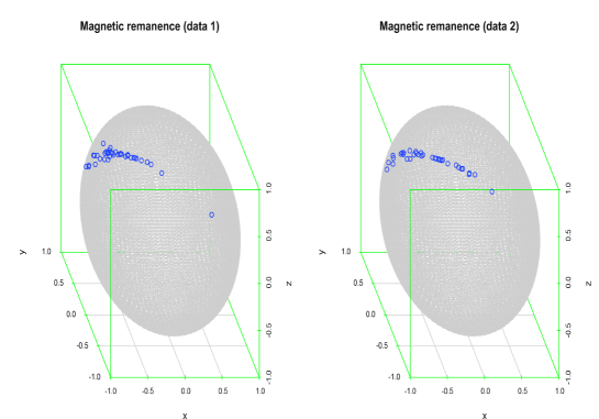
Figure 1: Measurements of remanent magnetization in red slits and claystones made at 2 different locations in Australia

Appendix

Proof of Proposition 4.1. From Watson (1983) (and the beginning of Section 2) we know that, under ${\rm P}^{(n)}_{{\boldsymbol{\vartheta}}_{0};\underline{g}}$, the sign vectors ${\bf S}_{{\boldsymbol{\theta}}}(\mathbf{X}_{ij})$ are independent of the scalar products $\mathbf{X}_{ij}^{\prime}{\boldsymbol{\theta}}$, ${\rm E}_{g_{i}}\left[{\bf S}_{{\boldsymbol{\theta}}}(\mathbf{X}_{ij})\right]=0$ and that

$${\rm E}_{g_{i}}\left[{\bf S}_{{\boldsymbol{\theta}}}(\mathbf{X}_{ij}){\bf S}_{{\boldsymbol{\theta}}}^{\prime}(\mathbf{X}_{ij})\right]=\frac{1}{k-1}({\bf I}_{k}-{\boldsymbol{\theta}}{\boldsymbol{\theta}}^{\prime})$$

for $i=1,\ldots,m$ and for all $j=1,\ldots,n_{i}$. These results readily allow to obtain Part (i) by applying the multivariate central limit theorem, while Part (ii) follows from the ULAN structure of the model in Proposition 3.1 and Le Cam’s third Lemma. $\square$

Proof of Proposition 4.2. We start by proving Part (i). First note that easy computations yield (for $i=1,\ldots,m$)

$${\boldsymbol{\Delta}}^{(n)}_{\hat{\boldsymbol{\theta}};\phi_{\kappa_{i}}} = \kappa_{i}n_{i}^{-1/2}\sum_{j=1}^{n_{i}}\left[\mathbf{X}_{ij}-(\mathbf{X}_{ij}^{\prime}\hat{\boldsymbol{\theta}})\hat{\boldsymbol{\theta}}\right]$$

$$= {\boldsymbol{\Delta}}^{(n)}_{{\boldsymbol{\theta}};\phi_{\kappa_{i}}}-\kappa_{i}n_{i}^{-1/2}\sum_{j=1}^{n_{i}}\left[(\mathbf{X}_{ij}^{\prime}\hat{\boldsymbol{\theta}})\hat{\boldsymbol{\theta}}-(\mathbf{X}_{ij}^{\prime}{\boldsymbol{\theta}}){\boldsymbol{\theta}}\right]$$

$$= {\boldsymbol{\Delta}}^{(n)}_{{\boldsymbol{\theta}};\phi_{\kappa_{i}}}-{\bf V}_{i}^{(n)}-{\bf W}_{i}^{(n)},$$

where ${\bf V}_{i}^{(n)}:=\kappa_{i}n_{i}^{-1}\sum_{j=1}^{n_{i}}\left[\mathbf{X}_{ij}^{\prime}{\boldsymbol{\theta}}\right]n_{i}^{1/2}(\hat{{\boldsymbol{\theta}}}-{\boldsymbol{\theta}})$ and ${\bf W}_{i}^{(n)}:=\hat{{\boldsymbol{\theta}}}\,\kappa_{i}n_{i}^{-1}(\sum_{j=1}^{n_{i}}\mathbf{X}_{ij}^{\prime})n_{i}^{1/2}(\hat{{\boldsymbol{\theta}}}-{\boldsymbol{\theta}})$. Now, combining the delta method (recall that ${\bf I}_{k}-{\boldsymbol{\theta}}{\boldsymbol{\theta}}^{\prime}$ is the Jacobian matrix of the mapping $h:\mathbb{R}^{k}\rightarrow\mathcal{S}^{k-1}:\mathbf{x}\mapsto\frac{\mathbf{x}}{\|\mathbf{x}\|}$ evaluated at ${\boldsymbol{\theta}}$), the Law of Large Numbers and Slutsky’s Lemma, we obtain that

$${\bf V}_{i}^{(n)} = \;\left(\kappa_{i}n_{i}^{-1}\sum_{j=1}^{n_{i}}\mathbf{X}_{ij}^{\prime}{\boldsymbol{\theta}}\right)n_{i}^{1/2}(\hat{{\boldsymbol{\theta}}}-{\boldsymbol{\theta}})$$

$$= \;\kappa_{i}{\rm E}_{g_{i}}[\mathbf{X}_{ij}^{\prime}{\boldsymbol{\theta}}]\;({\bf I}_{k}-{\boldsymbol{\theta}}{\boldsymbol{\theta}}^{\prime})n_{i}^{1/2}(\hat{{\boldsymbol{\theta}}}-{\boldsymbol{\theta}})+o_{\rm P}(1)$$

$$= {\boldsymbol{\Gamma}}_{{\boldsymbol{\theta}};g_{i}}^{\phi_{\kappa_{i}}}n_{i}^{1/2}(\hat{{\boldsymbol{\theta}}}-{\boldsymbol{\theta}})+o_{\rm P}(1)$$

under ${\rm P}^{(n)}_{{\boldsymbol{\vartheta}}_{0};\underline{g}}$ as $n\rightarrow\infty$. Thus, the announced result follows as soon as we have shown that ${\bf W}_{i}^{(n)}$ is $o_{\rm P}(1)$ under ${\rm P}^{(n)}_{{\boldsymbol{\vartheta}}_{0};\underline{g}}$ as $n\rightarrow\infty$. Using the same arguments as for ${\bf V}_{i}^{(n)}$, we have under ${\rm P}^{(n)}_{{\boldsymbol{\vartheta}}_{0};\underline{g}}$ and for $n\rightarrow\infty$ that

$${\bf W}_{i}^{(n)} = \hat{\boldsymbol{\theta}}\,\left(\kappa_{i}n_{i}^{-1}\sum_{j=1}^{n_{i}}\mathbf{X}_{ij}^{\prime}\right)n_{i}^{1/2}(\hat{{\boldsymbol{\theta}}}-{\boldsymbol{\theta}})$$

$$= \hat{\boldsymbol{\theta}}\,\left(\kappa_{i}n_{i}^{-1}\sum_{j=1}^{n_{i}}(\mathbf{X}_{ij}^{\prime})\;({\bf I}_{k}-{\boldsymbol{\theta}}{\boldsymbol{\theta}}^{\prime})\right)n_{i}^{1/2}(\hat{{\boldsymbol{\theta}}}-{\boldsymbol{\theta}})+o_{\rm P}(1)$$

$$= \hat{\boldsymbol{\theta}}\;\kappa_{i}{\rm E}_{g_{i}}\left[\sqrt{1-(\mathbf{X}_{ij}^{\prime}{\boldsymbol{\theta}})^{2}}({\mathbf{S}}_{{\boldsymbol{\theta}}}(\mathbf{X}_{ij}))^{\prime}\right]n_{i}^{1/2}(\hat{{\boldsymbol{\theta}}}-{\boldsymbol{\theta}})+o_{\rm P}(1),$$

which is $o_{\rm P}(1)$ from the boundedness of $\hat{\boldsymbol{\theta}}$ and since from Watson (1983) (see the proof of Proposition 4.1 for more details) we know that

$${\rm E}_{g_{i}}\left[\sqrt{1-(\mathbf{X}_{ij}^{\prime}{\boldsymbol{\theta}})^{2}}({\mathbf{S}}_{{\boldsymbol{\theta}}}(\mathbf{X}_{ij}))^{\prime}\right]={\rm E}_{g_{i}}\left[\sqrt{1-(\mathbf{X}_{ij}^{\prime}{\boldsymbol{\theta}})^{2}}\right]{\rm E}_{g_{i}}\left[({\mathbf{S}}_{{\boldsymbol{\theta}}}(\mathbf{X}_{ij}))^{\prime}\right]={\boldsymbol{0}}^{\prime}.$$

This concludes Part (i) of the proposition. Regarding Part (ii), let $\mathbf{X}$ be a random vector distributed according to an FvML distribution with concentration $\kappa$. Then, writing $c$ for the normalization constant, a simple integration by parts yields

$$C_{k,\phi_{\kappa}}=\kappa\,{\rm E}_{\phi_{\kappa}}[1-(\mathbf{X}^{\prime}{\boldsymbol{\theta}})^{2}] = \kappa\,c\int_{-1}^{1}(1-u^{2})\;{\rm exp}(\kappa u)(1-u^{2})^{(k-3)/2}\;du$$

$$= \kappa\,c\int_{-1}^{1}\;{\rm exp}(\kappa u)(1-u^{2})^{(k-1)/2}\;du$$

$$= c(k-1)\int_{-1}^{1}u\;{\rm exp}(\kappa u)(1-u^{2})^{(k-3)/2}\;du$$

$$= (k-1)\;{\rm E}_{\phi_{\kappa}}[\mathbf{X}^{\prime}{\boldsymbol{\theta}}].$$

The claim thus holds. $\square$

Proof of Proposition 4.3. We start the proof by showing that the replacement of ${\boldsymbol{\theta}}$ with $\hat{{\boldsymbol{\theta}}}$ as well as the distinct estimators have no asymptotic cost on $Q^{(n)}$. The consistency of $\hat{D}_{k,g_{i}}$, $\hat{E}_{k,g_{i}}$, $i=1,\ldots,m$, and $\hat{H}_{\underline{\phi},\underline{g}}$ together with the $n^{1/2}({\boldsymbol{\nu}}^{(n)})^{-1}$-consistency of $\hat{{\boldsymbol{\vartheta}}}$ entail that, using Part (i) of Proposition 4.2,

$$Q^{(n)}=\left({\boldsymbol{\Delta}}^{(n)}_{{\boldsymbol{\vartheta}}_{0};\underline{\phi}}-{\boldsymbol{\Gamma}}_{{\boldsymbol{\vartheta}}_{0};\underline{g}}^{\underline{\phi}}{\boldsymbol{\Upsilon}}^{(n)}\sqrt{n}\left(\hat{\boldsymbol{\theta}}-{\boldsymbol{\theta}}\right)\right)^{\prime}{{\boldsymbol{\Gamma}}}_{{\boldsymbol{\vartheta}}_{0};\underline{\phi},\underline{g}}^{\perp}\left({\boldsymbol{\Delta}}^{(n)}_{{\boldsymbol{\vartheta}}_{0};\underline{\phi}}-{\boldsymbol{\Gamma}}_{{\boldsymbol{\vartheta}}_{0};\underline{g}}^{\underline{\phi}}{\boldsymbol{\Upsilon}}^{(n)}\sqrt{n}\left(\hat{\boldsymbol{\theta}}-{\boldsymbol{\theta}}\right)\right)+o_{\rm P}(1)$$

under ${\rm P}^{(n)}_{{\boldsymbol{\vartheta}}_{0};\underline{g}}$ as $n\rightarrow\infty$. Now, standard algebra yields that

$${{\boldsymbol{\Gamma}}}_{{{\boldsymbol{\theta}}};\underline{\phi},\underline{g}}^{\perp}{\boldsymbol{\Gamma}}_{{\boldsymbol{\vartheta}}_{0};\underline{g}}^{\underline{\phi}}{\boldsymbol{\Upsilon}}^{(n)}=({\boldsymbol{\Gamma}}_{{\boldsymbol{\vartheta}}_{0};\underline{g}}^{\underline{\phi}}{\boldsymbol{\Upsilon}}^{(n)})^{\prime}{{\boldsymbol{\Gamma}}}_{{\boldsymbol{\vartheta}}_{0};\underline{\phi},\underline{g}}^{\perp}={\bf 0},$$

so that

$$Q^{(n)} = \left({\boldsymbol{\Delta}}^{(n)}_{{\boldsymbol{\vartheta}}_{0};\underline{\phi}}\right)^{\prime}{{\boldsymbol{\Gamma}}}_{{\boldsymbol{\vartheta}}_{0};\underline{\phi},\underline{g}}^{\perp}{\boldsymbol{\Delta}}^{(n)}_{{\boldsymbol{\vartheta}}_{0};\underline{\phi}}+o_{\rm P}(1)$$

$$=: Q^{(n)}({\boldsymbol{\vartheta}}_{0})+o_{\rm P}(1).$$

Both results from Proposition 4.1 entail that since ${\boldsymbol{\Gamma}}_{{\boldsymbol{\vartheta}}_{0};\underline{g}}^{*}{{\boldsymbol{\Gamma}}}_{{\boldsymbol{\vartheta}}_{0};\underline{\phi},\underline{g}}^{\perp}$ is idempotent with trace $(m-1)(k-1)$, $Q^{(n)}({\boldsymbol{\theta}})$ (and therefore $Q^{(n)}$) is asymptotically chi-square with $(m-1)(k-1)$ degrees of freedom under ${\rm P}^{(n)}_{{\boldsymbol{\vartheta}}_{0};\underline{g}}$, and asymptotically non-central chi-square, still with $(m-1)(k-1)$ degrees of freedom, and with non-centrality parameter $\mathbf{t}^{\prime}{\boldsymbol{\Gamma}}_{{\boldsymbol{\vartheta}}_{0};\underline{\phi},\underline{g}}{{\boldsymbol{\Gamma}}}_{{{\boldsymbol{\theta}}};\underline{\phi},\underline{g}}^{\perp}{\boldsymbol{\Gamma}}_{{\boldsymbol{\vartheta}}_{0};\underline{\phi},\underline{g}}\mathbf{t}$ under ${\rm P}^{(n)}_{{\boldsymbol{\vartheta}}_{0}+n^{-1/2}{\boldsymbol{\nu}}^{(n)}\mathbf{t}^{(n)};\underline{g}}$. Parts (i) and (ii) follow. Now, Part (iii) is a direct consequence of Part (i). Part (ii) of Proposition 4.2 and simple computations yield that $Q^{(n)}$ is asymptotically equivalent to the most stringent FvML test $Q_{\underline{\phi}}^{(n)}$ in (3.7). Part (iv) thus follows. $\square$

Acknowledgements

The research of Christophe Ley is supported by a Mandat de Chargé de Recherche from the Fonds National de la Recherche Scientifique, Communauté française de Belgique.

References

• Acton (2011) Acton, G. (2011). Essentials of Paleomagnetism. Eos Trans. AGU 92, 166 pages.
• Beran and Fisher (1998) Beran, R. and Fisher, N. I. (1998). Nonparametric comparison of mean directions or mean axes. Ann. Statist. 26, 472–493.
• Bingham and Mardia (1975) Bingham, M. S. and Mardia, K. V. (1975). Characterizations and applications. In S. Kotz, G. P. Patil and J. K. Ord, eds, Statistical Distributions for Scientific Work, volume 3, Reidel, Dordrecht and Boston, 387–398.
• Breitenberger (1963) Breitenberger, E. (1963). Analogues of the normal distribution on the circle and the sphere. Biometrika 50, 81–88.
• Chang (2004) Chang, T. (2004). Spatial statistics. Statist. Sci. 19, 624–635.
• Duerinckx and Ley (2013) Duerinckx, M. and Ley, C. (2013). Maximum likelihood characterization of rotationally symmetric distributions. Sankhyā Ser. A, to appear.
• Embleton and Mc Donnell (1980) Embleton, B. J. J. and Mc Donnell, K.L. (1980). Magnetostratigraphy in the Sidney Basin, Southern Australia. J. Geomag. Geoelectr. 32, Suppl. III (304).
• Fisher (1953) Fisher, R. A. (1953). Dispersion on a sphere. Proceedings of the Royal Society of London, Ser. A 217, 295–305.
• Fisher and Hall (1990) Fisher, N.I. and Hall, P. (1990). New statistical methods for directional data I. Bootstrap comparison of mean directions and the fold test in palaeomagnetism. Geophys. J. Int. 101, 305–313.
• Fisher, Lewis and Embleton (1987) Fisher, N. I., Lewis, T., and Embleton, B. J. J. (1987). Statistical Analysis of Spherical Data. Cambridge University Press, UK.
• Hallin and Paindaveine (2008) Hallin, M. and Paindaveine, D. (2008). A general method for constructing pseudo-Gaussian tests. J. Japan Statist. Soc. 38, 27–39.
• Hallin et al. (2010) Hallin, M., Paindaveine, D. and Verdebout, T. (2010). Optimal rank-based testing for principal components. Ann. Stat. 38, 3245–3299.
• Kreiss (1987) Kreiss, J. P. (1987). On adaptive estimation in stationary ARMA processes. Ann. Stat. 15, 112–133.
• Langevin (1905) Langevin, P. (1905). Sur la théorie du magnétisme. J. Phys. 4, 678–693; Magnétisme et théorie des électrons. Ann. Chim. Phys. 5, 70–127.
• Le Cam (1986) Le Cam, L. (1986). Asymptotic Methods in Statistical Decision Theory. Springer-Verlag, New York.
• Le Cam and Yang (2000) Le Cam, L. and Yang, G. L. (2000). Asymptotics in Statistics, 2nd edition. Springer-Verlag, New York.
• Leong and Carlile (1998) Leong, P. and Carlile, S. (1998). Methods for spherical data analysis and visualization. J. Neurosci. Meth. 80, 191–200.
• Ley et al. (2013) Ley, C., Swan, Y., Thiam, B. and Verdebout, T. (2013). Optimal $R$-estimation of a spherical location. Stat. Sinica 23, to appear.
• Mardia and Jupp (2000) Mardia, K. V. and Jupp, P. E. (2000). Directional Statistics. Wiley, New York.
• McFadden and Jones (1981) McFadden, P. L. and Jones, D. L. (1981). The fold test in palaeomagnetism. Geophys. J. R. Astron. Soc. 67, 53–58.
• Merrifield (2006) Merrifield, A.J. (2006). An Investigation Of Mathematical Models For Animal Group Movement, Using Classical And Statistical Approaches, Phd-thesis, University of Sydney.
• Muirhead and Waternaux (1980) Muirhead, R. J. and Waternaux, C. M. (1980). Asymptotic distributions in canonical correlation analysis and other multivariate procedures for nonnormal populations. Biometrika 67, 31–43.
• Saw (1978) Saw, J. G. (1978). A family of distributions on the $m$-sphere and some hypothesis tests. Biometrika 65, 69–73.
• Schaeben (1992) Schaeben, H. (1992). “Normal” orientation distributions. Textures Microstruct. 19, 197–202.
• Watson (1983) Watson, G. S. (1983). Statistics on Spheres. Wiley, New York.
• Wellner (1979) Wellner, J. A. (1979). Permutation tests for directional data. Ann. Statist. 7, 929–943.